a heuristic approach for resource constrained project scheduling with uncertain activity durations
TRANSCRIPT

Computers & Operations Research 38 (2011) 1305–1318
Contents lists available at ScienceDirect
Computers & Operations Research
0305-05
doi:10.1
� Corr
E-m
journal homepage: www.elsevier.com/locate/caor
A heuristic approach for resource constrained project scheduling withuncertain activity durations
M.E. Bruni �, P. Beraldi, F. Guerriero, E. Pinto
Universit �a degli Studi della Calabria, 87030 Rende (CS), Italy
a r t i c l e i n f o
Available online 10 December 2010
Keywords:
Resource constrained project scheduling
Random activity duration
Heuristic
Joint chance constraints programming
48/$ - see front matter & 2010 Elsevier Ltd. A
016/j.cor.2010.12.004
esponding author. Tel.: +39 984 494038; fax
ail address: [email protected] (M.E. Brun
a b s t r a c t
In this paper, we address the resource constrained project scheduling problem with uncertain activity
durations. Project activities are assumed to have known deterministic renewable resource requirements
and uncertain durations, described by independent random variables with a known probability
distribution function. To tackle the problem solution we propose a heuristic method which relies on a
stage wise decomposition of the problem and on the use of joint probabilistic constraints.
& 2010 Elsevier Ltd. All rights reserved.
1. Introduction
The resource constrained project scheduling problem (RCPSP)consists in minimizing the duration of a project, subject toprecedence and resource constraints. In its deterministic version,the RCPSP assumes complete information on the resource usageand activities duration, and determines a feasible baseline sche-dule, i.e. a list of activity starting times, minimizing the makespanvalue. The importance of the baseline schedule has been widelyrecognized in Aytug et al. [1] and Mehta and Uzsoy [2] as valuablesupport for project decision makers in resources allocation andexternal activities planning. Very often, the baseline schedule isbuilt considering average values for activities durations andresource requirements. However, in real contexts, this simplifica-tion may lead to very poor performance, since project executionmay be subject to severe uncertainty and then may undergo severaltypes of disruptions as described in Wang [3] and Zhu et al. [4].
Extensions of the RCPSP, involving the minimization of the expectedmakespan of a project with stochastic activity durations, have beeninvestigated within the stochastic project scheduling literature. Sincethe problem is rather involved, scheduling policies [5–7] and heuristicprocedures [8–11] have been used for defining which activities to startat random decision points through time, based on statistical knowledgeabout the random durations distributions.
Beside this important research stream, the field of proactiveproject scheduling has received outstanding attention in the lastyears. In this approach, some knowledge of the uncertainty isincorporated in the decision-making stage, with the aim to gen-erate predictive schedules that are in some sense insensitive tofuture adverse events.
ll rights reserved.
: +39 984 494847.
i).
Van De Vonder et al. [12,13] propose the so-called resourceflow-dependent float factor heuristic (RFDFF) to obtain a prece-dence and resource feasible schedule, using information comingfrom the resource flow network [14] in the calculation of the socalled activity dependent float factor [15]. In Van de Vonder et al.[16], several predictive reactive resource constrained projectscheduling procedures are evaluated under the composite objec-tive of maximizing both the schedule stability and the timelyproject completion probability. For an extensive review of researchin this field, the reader is referred to Herroelen and Leus [17,18].Within this research stream, and when abstraction of resourceusage is made, we mention the works of Herroelen and Leus [19],Rabbani et al. [20], Tavares et al. [21].
When resource availability constraints are considered, Leus andHerroelen [22], Deblaere et al. [23] and Lambrechts et al. [24,25]assuming the availability of a feasible baseline schedule, proposedexact and approximate formulations of the robust resource allocationproblem.
Within the stochastic programming context, a two-stage inte-ger linear stochastic model has been proposed in Zhu et al. [26].Target times are determined in the first stage followed by thedevelopment of a detailed project schedule in the second stage. Thetwo-stage stochastic model aims at minimizing the cost of projectcompletion and expected penalty incurred by deviating from thespecified values. Only one non-renewable resource (the budget) isconstrained in the model. A path-based two-stage integer pro-gramming approach, together with a tailored solution methodol-ogy based on decomposition, has been recently proposed byKlerides and Hadjiconstantinou [27] for the stochastic discretetime-cost trade-off problem. The more difficult case involvingmultiple renewable resources has not been investigated yet in thestochastic programming setting.
This paper addresses the case of RCPSP with renewable resourcesand uncertain activities durations represented by independent random

M.E. Bruni et al. / Computers & Operations Research 38 (2011) 1305–13181306
variables with known cumulative probability distribution function. Theobjective is to build a precedence and resource feasible baselineschedule with minimum makespan able to tolerate a certain degreeof uncertainty during execution and to absorb dynamic variations inactivities durations (we shall refer in the following to this capability asstability or robustness). Our ultimate aim is to develop a projectscheduling procedure capable of combining schedule stability andmakespan performance. There are a number of different metrics forassessing the robustness of a schedule in literature. In this paper weadopt as a measure the probability that schedule decisions do notchange during execution. In particular, through the use of jointprobabilistic constraints, we try to find a schedule that is expectedto be respected with a high level of probability. The use of jointprobabilistic constraints, within the stochastic scheduling problem,represents an innovative element of our approach. In effect, at the bestof our knowledge, none of the methods proposed in the literatureconsiders joint probabilistic constraints. Indeed, very few researchpapers explicitly consider probabilistic information in solution meth-ods. We should mention here, the work of Van de Vonder et al. [28]where the virtual activity duration extension (VADE) heuristic and thestarting time criticality (STC) heuristic are introduced to include timebuffers in a given schedule while a predefined project due date remainsrespected. While VADE heuristic relies on the standard deviation of theduration of an activity in order to compute a modified duration, STCheuristic tries to combine information on activity weights and on theprobability that activity cannot be started at its scheduled starting time.
Our work differs from the cited paper in some important aspects.First of all, we consider the stochastic programming framework and, inparticular, the probabilistic paradigm in the form of joint probabilisticconstraints. This powerful tool allows us to relax the assumption,common in the literature, that only one activity at a time disturbs thestarting time of a successor activity, rather limiting the joint probabilityof disruption of the preceding activities to a given probability level.In addition, we do not start from an initial deterministic unbufferedschedule in which to insert time buffers, although starting from anunbuffered schedule is a very common practice amongst practitionersand researchers. Last, but not least, our point of view is rather new inthe literature on predictive stable scheduling procedures where theobjective function commonly used (see for instance Leus, [15]) is the socalled stability cost function, defined as the weighted sum of theexpected absolute deviation between the actually realized activity starttimes and the planned activity start times. We observe that thisobjective function is not known a priori, unless a range of executionscenarios (referred to as the training set) are simulated by drawingdifferent actual activities durations from the described distributionfunctions. In addition, it is not difficult to see that the exact quantifica-tion of the deviation between planned and actual starting times heavilydepends on the reactive procedure adopted.
The remainder of the paper is organized as follows. In Section 2we describe our scheduling methodology for generating robustbaseline schedules. Section 3 is devoted to the presentation ofcomputational experiments and conclusions are given in Section 4.
2. Project scheduling with uncertain activity durations
2.1. Notation and problem description
We assume that the activity network of a resource constrainedproject in activity-on-node representation is given by a directed acyclicgraph A¼(N,V). Each node in the set N¼{0,y,n+1} corresponds to asingle project activity and each arc in the set V corresponds to aprecedence relation between each pair of activities [29]. The nodes0 and n+1 are the dummy start and the dummy end activities,respectively. For each activity jAN, FSj denotes the set of successoractivities of j, whereas BSj denotes the set of its predecessor activities.
We assume the presence of a set of K renewable resources with aper-period availability ak. Each activity jAN has to be processedwithout interruptions, requiring a constant amount of resource rjk
for each renewable resource type k, k¼1,y,K. We assume thatactivities durations are uncertain and we denote by dðoÞ the vectorof random variables defined on a given probability space Oequipped with an algebra F and with a probability measure P.Then, the random vector of starting times can be denoted withsðoÞ ¼ ðs0ðoÞ, . . . ,snþ1ðoÞÞ and the associated random vector ofcompletion times with f ðoÞ ¼ ðf 0ðoÞ, . . . , f nþ1ðoÞÞ.
In uncertain environments, especially from a practical point ofview, project managers are mainly interested in the generation of aproactive schedule (i.e. a vector of proactive starting timess¼ ðs0, . . . ,snþ1Þ and finish times f¼ ðf0, . . . ,fnþ1Þ) with a qual-ity that does not degrade during execution with respect to futureperturbations. The vector s can be interpreted as the mapping ofrandom activity durations into a vector of resource and precedencefeasible starting times performed according to a function P :
O-Rþnþ1 referred as policy.During the execution of a project, the realized starting time of an
activity may be different from its predictive starting time. Thecorresponding deviation is still a random variable defined for ageneric activity j as follows:
DjðoÞ ¼s jðoÞ�sj if s jðoÞ�sj40
0 otherwise
( ):
Two classical approaches can be used to deal with randomdeviations. Unit penalty costs can be assigned for each individualdeviation, and the resulting expected penalty cost can be mini-mized, or alternatively, one may specify a model in which weaccept the risk of deviations with a certain probability.
From a mathematical standpoint, risk averse constraints can beformulated by using the theory of joint probabilistic constraints asin the sequel.
PðDjðoÞ40, 8jANÞre: ð1Þ
This probabilistic constraint can be interpreted as a robustnessconstraint limiting from above the probability of a scheduledisruption by the parameter eA ½0,1�.
Though appealing, determining a policyP and a vector of predictivestarting times s such that the makespan CmaxðPÞ ¼ snþ1 of theschedule is minimized and constraint (1) is fulfilled is cumbersomefrom a theoretical and a computational point of view. Rather thantackling the full complex stochastic dynamic problem presented above,in this study, we propose to address scheduling robustness by a methodthat decouples the dynamic aspect from the stochastic one reconcilingtheir benefits through the use of stochastic information. In particular, astochastic dynamic generation scheme identifies and resolves theresource allocation decisions whilst stochastic constraints capture theuncertainty in activity durations by taking into account a robustnessconstraint. The ultimate objective is still the minimization of the projectmakespan.
It is easy to recognize that the topic addressed in this paper isclosely related to the issue of solution stability addressed in Van deVonder et al. [12], also refereed as solution robustness. Whilstrobustness has been considered in the literature mainly as anobjective to pursuit, in our paper we introduce a different point ofview, considering robustness as a soft constraint to satisfy at eachconsidered decision point.
2.2. The stochastic dynamic schedule generation scheme
In this section we shall present the stochastic dynamic decisionprocess to tackle the problem under study. Decisions to be madeconcern which activities to start at certain decision points by tacking

M.E. Bruni et al. / Computers & Operations Research 38 (2011) 1305–1318 1307
into account the resources availability. A decision point occurs either atthe beginning of the project, or when at least one of the runningactivities is completed, until the last activity is scheduled. At eachdecision point, a resource feasible partial schedule is built and suitableproactive starting and completion times are set by means of ananticipative stochastic model that accounts for future uncertainty.Since the policy we use can be viewed as a stochastic dynamic versionof the parallel schedule generation scheme, it is easy to verify that thepartial schedule constructed is feasible with respect to precedence andresource constraints.
A detailed description of the proposed stochastic dynamicgeneration scheme (SDGS) heuristic is given in what follows. Letus denote with:
�
g the iteration counter; � tg the decision time associated with iteration g; � Cg the set of activities already scheduled and completed up to tg; � Ag the set of activities which are active at tg; � Eg the set of activities whose predecessors BSj have beencompleted at time tg;
� Sg a subset of Eg containing activities that will start at time tg; � Rk(tg) the residual resource availability at time tg; � r a priority rule.An algorithmic description of the SDGS heuristic is given below.
Algorithm. Scheme of the SDGS heuristic
InitializationSet g :¼ 0, t0 :¼ 0, C0 :¼ fg, E0 :¼ fg, A0 :¼ f0g, S0 :¼ f0g, f0 ¼ t0,
s0 ¼ t0 Rkðt0Þ :¼ ak, k¼1, y, K
Choice a priority rule rRepeat until jCg [ Ag j ¼ nþ1
g :¼ gþ1
tg :¼ minjAAg�1fj
Cg :¼ Cg�1 [ fjAAg�1jfjrtgg
Ag :¼ fjANjfj4tgg
Eg :¼ fjAN\ðCg [ AgÞjBSjDCgg
Sg :¼ fg
RkðtgÞ :¼ ak�P
jAAgrjk
While Eg afgUse the priority rule r to select a new activity jAEg to be
scheduled
Eg :¼ Eg\fjg
If j is such that RkðtgÞ�rjkZ0 then
Sg :¼ Sg [ fjg
Ag :¼ Ag [ fjg
RkðtgÞ :¼ RkðtgÞ�rjk
sj :¼ tg
End ifEnd While
Determine the proactive completion times fj,8jASg
End Repeat
2.3. Generating activities completion times
While the dynamic aspect of the problem is tackled at decisionpoints by the scheduling policy presented above, the stochasticity istaken into account in the determination of proactive starting andcompletion times.
We recall that at each decision point tg, our decisions concern theappropriate proactive completion times of activities in Sg since thestarting times of activities jASg are set assj ¼ tg , where tg represents acompletion time of one previously scheduled activity. As a reminder,
we notice that these decisions should ensure the satisfaction of thestability constraint (1) at each decision point. We now observe thatpotentially any activity in Ag could cause a disruption among itssuccessor, since its completion time represents the new decision pointat which an unscheduled activity l should set its starting time sl. Wefurther notice that, at the time we take decisions, we do not knowwhich activities would be scheduled in the next stage, nor what will bethe next decision point.
Therefore, at a generic instant tg rtrtgþ1, the probability ofnot causing a disruption in the schedule in the future is theprobability that for any activity i currently under execution(iAAg) the condition fiZ f iðoÞ is verified.
Now, we may conclude that the problem boils down in appro-priately setting completion times by solving at each decision pointtg the following problem with joint chance constraints:
min Mpar ð2Þ
Mpar Zfi 8iASg ð3Þ
PðfiZtgþ diðoÞ 8iASgÞZð1�eÞ ð4Þ
where Mpar represents the makespan of the partial schedule builtconsidering activities iASg and tgþ diðoÞ ¼ f iðoÞ8iASg . Here jointchance constraints are imposed to set the completion time of theactivities, at each decision point, in such a way that the probabilityof not disrupting the schedule in the future is at least ð1�eÞ (i.e. therisk of disruption is at most e). We emphasize that completiontimes of the activities in Ag\Sg have been set appropriately at aprevious decision point.
In order to show how the heuristic works, a toy example isreported in Appendix A.
We should point out that if, at least in principle, separate chanceconstraints can be used to deal with uncertain durations, thesolution provided by the corresponding model may in somecontext be considered inappropriate. In fact, imposing a smallprobability of disruption for each activity jASg does not assure asmall joint probability for all jASg .
It is worth observing that, although at each decision point we acceptthe risk of a disruption with probability e, we cannot impose a limit onthe probability of not completing the whole project on time. However,we may express the timely project completion probability as a functionof the number of decision points performed by the algorithm. A crudelower bound for the probability of project to be completed on time isð1�eÞG where G is an upper bound on the number of iterations.
2.4. Solving the joint probabilistically constrained problem
The SDGS heuristic involves the repeated solution of model(2)–(4). In the following, we show how to derive a deterministicequivalent formulation, in the case of independent randomvariables.
Under the independence assumption among the random vari-ables diðoÞ, the probabilistic constraints (4) can be rewritten asYiA Sg
PðfiZtgþ diðoÞÞZ ð1�eÞ: ð5Þ
Denoting with FdiðoÞ
the marginal probability distribution functionof the random variable diðoÞ, and with a variable substitutionci ¼fi�tg , constraints (5) can be stated equivalently asYiA Sg
FdiðoÞðciÞZð1�eÞ
and by taking logarithms:XiA Sg
lnFdiðoÞðciÞZ lnð1�eÞ

M.E. Bruni et al. / Computers & Operations Research 38 (2011) 1305–13181308
(see, for example Jagannathan [30] and Miller and Wagner [31]).Since the logarithm is an increasing function and 0oF
diðoÞr1,
this transformation is legitimate. Furthermore, for log-concavedistribution functions, convexity of the constraints is preserved.The class of log-concave random variables includes several com-monly used probability distributions as for example the Uniform,Normal, Exponential and many others (see Prekopa, [32] andDentcheva et al. [33]). We observe that also in the case of discretedistributions, problems with joint probabilistic constraints can bereduced to deterministic equivalent problems. For more details, theinterested readers are referred to Dentcheva et al. [33] (In AppendixA the transformation is detailed for illustrative purposes).
Therefore, depending on the continuous or discrete nature of therandom variables involved in the problem, the deterministicequivalent problem takes the form of a nonlinear continuousproblem or a linear integer problem.
3. Computational experiments
Extensive numerical experiments have been carried out with theaim of assessing the performance of the SDGS heuristic. A comparativeevaluation has also been made with a set of benchmark heuristics thatwe shall present in the next paragraph.
3.1. Benchmark approaches
In order to assess the performance of the proposed SDGSheuristic, we have considered for comparison a set of schedulingprocedures based on the use of separate chance constraints. Morespecifically, both parallel schedule generation schemes (PSGS) andserial schedule generation schemes (SSGS) have been designed byreplacing deterministic durations by their ð1�eÞ-quantile counter-parts ðF�1
d jðoÞð1�eÞÞ. We should remark that this is equivalent of using
separate chance constraints within classical schedule generationheuristics for the deterministic RCPSP. The following static priorityrules for generating the priority list have been tested:
1.
(MaxC) The MaxC rule orders the activities jAN by decreasingvalue of their total resource requirement rðjÞ ¼PK
k ¼ 1 rjk.
2.
(MinC) The MinC rule orders the activities jAN by increasingvalue of their total resource requirement rðjÞ ¼PK
k ¼ 1 rjk.
3.
(MaxDnC) The MaxDnC rule orders the activities by decreasingvalue of F�1d jðoÞð1�eÞ�rðjÞ with rj defined as above.
4.
(MinD) The MinD rule orders the activities by increasing value ofF�1d jðoÞð1�eÞ.
5.
(LST) The LST rule orders the activities by increasing value oftheir latest starting time LSj as described in Kolisch andHartmann [34].6.
(LFT) The LFT orders the activities by increasing value of theirlatest finish time LFj as described in Davis and Patterson [35].7.
1 10 problems with 30 activities (j301-1,j3010-10, j3044-1, j305-1, j306-1,
j306-1, j307-1, j308-1,j309-7, j3037-4), 10 problems with 60 activities (j601-1,
j602-1, j6030-10, j6048-1, j6048-9, j605-1, j606-1, j607-1, j608-1, j609-1), and 10
problems with 90 activities (j901-1, j9010-1,j9018-8, j9020-10, j9047-1, j905-1,
j906-1, j907- 1, j908-1,j909-1).
(MTS) The MTS orders the activities by decreasing value of thenumber of their successors, that is jFSjj as described in Alvarez–Valdes and Tamarit [36].
Whilst the last three rules have been taken from the literature [34],the other rules have been proposed by the authors. Moreover, wehave considered the STC [28] and the RFDFF heuristic [13].
3.2. Computational results
The computational experiments have been performed on a PCPentium III, 667 MHz, 256 MB of RAM. All procedures were codedin AIMMS language (Bisschop and Roelofs, [37]) and the
subproblems solved with Cplex 10.1 (ILOG CPLEX 6.5: UsersManual, [38]) and Conopt [39]. Algorithms 1–4 are the PSGS withthe first four priority rules, algorithms 5–8 are the SSGS with thesame priority rules, algorithms from 9 to 11 are PSGS with the rulesLST, LFT and MTS, respectively. The SDGS heuristic procedure hasbeen executed considering the four priority rules MaxC, MinC,MaxDnC and MinD (algorithms A–D) since they behave the best.The STC and RFDFF heuristic algorithms consider a deterministicproject due date and start from a minimum makespan schedule inwhich time buffers are inserted in order to protect againstanticipated disruptions. The unbuffered baseline schedule requiredby the STC and RFDFF heuristics has been obtained by applyingalgorithm 4 (PSGS heuristic with MinD rule) with different e values(this choice has been motivated by the fact that SDGS heuristic is astochastic version of the PSGS), whereas the project due date hasbeen set equal to the average makespan obtained by algorithmsA–D. The instability weights have been considered equal to one forall the activities, except for the final one for which the weight hasbeen set equal to 10 as suggested in Van de Vonder et al. [28]. Thisparticular setting reflects the fact that in our heuristic theprobabilistic constraints are imposed on all the activities withthe same value for the risk parameter e which, in turn, implies thatall the activities are considered equally important. Furthermore,since the objective of our heuristic is the makespan minimization,the weight of the last activity has been set to 10 in order to givemore emphasis on the project makespan (in this respect it could bebeneficial to recall that the weight of the dummy end activitydenotes the cost of delaying the project completion beyond apredefined deterministic project due date). For the STC heuristicthe stability cost improvement has been evaluated on a training setof 100 scenarios.
All the scheduling procedures have been executed for five valuesof e namely {0.2,0.15,0.1,0.05,0.01}.
The computational experiments have been carried out on a set1 ofbenchmark problems selected from the project scheduling problemlibrary PSPLIB [40], available at http://129.187.106.231/psplib/, includ-ing 30, 60 and 90 nodes, leading to a total of 2550 runs.
For all the instances, two types of distribution have been testedin order to asses the effectiveness of the proposed approach withboth continuous and discrete distributions.
In particular, for the continuous case, we have assumed that realactivity duration is a uniform random variable U(0.75 d, 2.85 d),where d has been set equal to the deterministic duration and for thediscrete case, we have considered a Poisson distribution with meand. Activity durations are assumed to be independent.
Extensive simulation has been carried out to evaluate allprocedures on robustness measures and computational efficiency.For every network instance, 1000 scenarios have been simulated bydrawing different actual activity durations from the describeddistribution functions. Using these simulated activity durations,the realized schedule is constructed by applying the followingreactive procedure. An activity list is obtained by ordering theactivities in increasing order of their starting times in the proactiveschedule. Ties are broken by increasing activity number. Relying onthis activity list, a parallel schedule generation scheme builds aschedule based on the actual activity durations. We opted for therailway execution mode [23] never starting activities earlier thantheir prescheduled start time in the baseline schedule. Actually,this type of constraint is inherent to course scheduling, sportstimetabling, railway and airline scheduling, or when activity

Fig. 1. e values versus Tavg.
Fig. 2. e values versus TPCP.
Fig. 3. Expected makespan for varying e values-30 nodes-Discrete case.
Fig. 4. Expected makespan for varying e values-60 nodes-Discrete case.
M.E. Bruni et al. / Computers & Operations Research 38 (2011) 1305–1318 1309
execution cannot start before the necessary resources have beendelivered.
3.3. Analysis of results
Rather than showing the complete set of the numerical results,fully reported in Beraldi et al. [41], we give in Tables 1–6 of theAppendix B, for each procedure, the average results calculated overall networks and executions. The quality has been evaluated by thefollowing a posteriori measures of stability: average tardiness(Tavg), average timely project completion probability (TPCP),average disruption probability over all networks and executions(Davg). Also the predictive makespan (Mak) has been reportedenabling a fair comparison amongst the different algorithms.
In the next subsection we will present our results for the discreteand the continuous case. Here we shall briefly comment on thecomputational times since they are rather low and do not constitutea bottleneck for the algorithms execution. In particular, the CPU timeis very limited for algorithms 1–11, given the simple scheduleconstruction procedures based on the parallel and serial schedulegeneration scheme. Also procedures A–D are competitive in terms oftimely performance, with CPU times varying from 0 to a couple ofseconds. The execution times of procedures A–D, is slightly higherthan the computational time of STC and RFDFF only for 90 nodesnetworks and discrete distribution. This is due to the extra effortrequired for solving, at each decision point, the integer lineardeterministic equivalent of the probabilistic model. For the con-tinuous case, the computational requirements for SDGS and the STCand RFDFF heuristics are roughly similar, although the model to besolved within the SDGS heuristic is a nonlinear continuous model.
In order to give an idea of the size of the probabilistic problemssolved within the SDGS heuristic, Table 7 reports the average,minimum and maximum number of variables and constraintsinvolved in the solution of problem (2)–(4) at each iteration of theSDGS heuristic for both the discrete and the continuous case. Forthe sake of completeness also the average number of iterationsperformed is reported. As evident a higher number of variables andconstraints characterises the integer deterministic equivalentproblems related to discrete random variables.
3.3.1. Discrete distribution
In this section, we comment on computational results obtainedfor the discrete case. A detailed accounting of the numerical resultsis reported in Tables 1–3.
A first set of numerical experiments has been carried out with theaim of assessing the variation of the performance measures of our SDGSalgorithm as a function of the risk level (measured by e).
We report in Figs. 1 and 2 the Tavg and the TPCP for different evalues, for the 30 nodes test problems. As we can observe in Fig. 1, theaverage tardiness decreases with e. This is an expected result since fordecreasing value of e we impose a more prudent project manager’sposition imposing a higher risk aversion level. Mathematically speak-ing, as the value of e decreases, probabilistic constraints are somehowmore binding and the schedule is more robust, since it is less exposedto disruptions. The opposite trend can be observed in Fig. 2 for theTPCP which increases for decreasing e values.
A second set of experiment has been carried out to compare theperformance of the SDGS with respect to the benchmark approachespresented in Section 3.1. In particular, we shall present hereafter agraphical comparison on the basis of the expected makespan EXPMAK,(obtained as the sum of the predictive makespan Mak plus the expectedtardiness Tavg) and the average probability of disruption Davg.
Figs. 3–5 show the EXPMAK for the 30, 60 and 90 nodesnetworks, respectively. Average values have been reported forthe procedures A–D (named SDGS) and 1–11 (named OTHERS). The
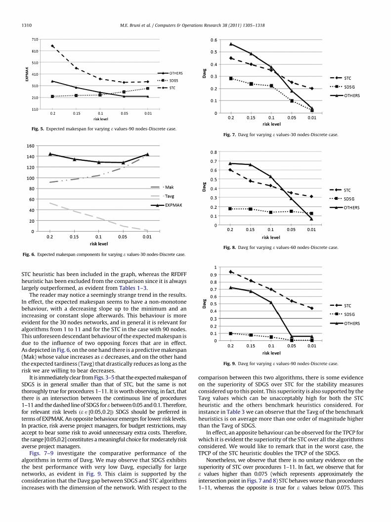
Fig. 5. Expected makespan for varying e values-90 nodes-Discrete case.
Fig. 6. Expected makespan components for varying e values-30 nodes-Discrete case.
Fig. 7. Davg for varying e values-30 nodes-Discrete case.
Fig. 8. Davg for varying e values-60 nodes-Discrete case.
Fig. 9. Davg for varying e values-90 nodes-Discrete case.
M.E. Bruni et al. / Computers & Operations Research 38 (2011) 1305–13181310
STC heuristic has been included in the graph, whereas the RFDFFheuristic has been excluded from the comparison since it is alwayslargely outperformed, as evident from Tables 1–3.
The reader may notice a seemingly strange trend in the results.In effect, the expected makespan seems to have a non-monotonebehaviour, with a decreasing slope up to the minimum and anincreasing or constant slope afterwards. This behaviour is moreevident for the 30 nodes networks, and in general it is relevant foralgorithms from 1 to 11 and for the STC in the case with 90 nodes.This unforeseen descendant behaviour of the expected makespan isdue to the influence of two opposing forces that are in effect.As depicted in Fig. 6, on the one hand there is a predictive makespan(Mak) whose value increases as e decreases, and on the other handthe expected tardiness (Tavg) that drastically reduces as long as therisk we are willing to bear decreases.
It is immediately clear from Figs. 3–5 that the expected makespan ofSDGS is in general smaller than that of STC, but the same is notthoroughly true for procedures 1–11. It is worth observing, in fact, thatthere is an intersection between the continuous line of procedures1–11 and the dashed line of SDGS for e between 0.05 and 0.1. Therefore,for relevant risk levels ðeA ½0:05,0:2�Þ SDGS should be preferred interms of EXPMAK. An opposite behaviour emerges for lower risk levels.In practice, risk averse project managers, for budget restrictions, mayaccept to bear some risk to avoid unnecessary extra costs. Therefore,the range [0.05,0.2] constitutes a meaningful choice for moderately riskaverse project managers.
Figs. 7–9 investigate the comparative performance of thealgorithms in terms of Davg. We may observe that SDGS exhibitsthe best performance with very low Davg, especially for largenetworks, as evident in Fig. 9. This claim is supported by theconsideration that the Davg gap between SDGS and STC algorithmsincreases with the dimension of the network. With respect to the
comparison between this two algorithms, there is some evidenceon the superiority of SDGS over STC for the stability measuresconsidered up to this point. This superiority is also supported by theTavg values which can be unacceptably high for both the STCheuristic and the others benchmark heuristics considered. Forinstance in Table 3 we can observe that the Tavg of the benchmarkheuristics is on average more than one order of magnitude higherthan the Tavg of SDGS.
In effect, an apposite behaviour can be observed for the TPCP forwhich it is evident the superiority of the STC over all the algorithmsconsidered. We would like to remark that in the worst case, theTPCP of the STC heuristic doubles the TPCP of the SDGS.
Nonetheless, we observe that there is no unitary evidence on thesuperiority of STC over procedures 1–11. In fact, we observe that fore values higher than 0.075 (which represents approximately theintersection point in Figs. 7 and 8) STC behaves worse than procedures1–11, whereas the opposite is true for e values below 0.075. This

Fig. 12. Expected makespan for varying e values-90 nodes-Continuous case.
M.E. Bruni et al. / Computers & Operations Research 38 (2011) 1305–1318 1311
suggests that there is a golden value for the risk parameter that couldguide the manager in the choice of the appropriate heuristic to use.
If solution stability is deemed of utmost importance, the bestchoice seems to be the SDGS heuristic. This heuristic guaranteesvery good stability performance in terms of disruption probability.If, on the contrary, the sensitivity of the schedule performance interms of the objective value is the criterion to pursuit, we observethat nice results are obtained for eZ0:01 by the STC heuristic withhigh TPCP and also acceptable stability indicators. When theproject manager is very conservative and risk averse (er0:05)an attractive alternative especially for large instances can beconstituted by procedures 1–11 that offer a good comprisebetween computational time and solution quality. However,above this risk level they fall inevitably in solutions of substantiallylower quality.
As a marginal note, we point out that the performances of thealgorithms 1–11 are barely indistinguishable and depend on theordering criterion adopted. Unfortunately, there is no unitaryevidence of one criterion over the others.
As far as the RFDFF is concerned, we observe that notwithstand-ing the unbuffered schedule fed into RFDFF depends on the e valueconsidered, the results obtained are almost the same whatever therisk aversion of the decision maker is. This behaviour can be due tothe right-justification mechanism, which insert buffers in front ofthe activities in order to make the schedule solution robust.
Fig. 13. TPCP for varying e values-60 nodes-Continuous case.
3.3.2. Continuous distribution
Tables 4–6 summarise the results for the continuous distribu-tion function. Some conclusions can be drawn on the basis of thenumerical results collected.
As before, we show in Figs. 10–12 the EXPMAK for the 30, 60 and90 nodes networks, respectively. We observe that the general trend
Fig. 10. Expected makespan for varying e values-30 nodes-Continuous case.
Fig. 11. Expected makespan for varying e values-60 nodes-Continuous case.
Fig. 14. Davg for varying e values-30 nodes-Continuous case,
is similar to the one observed for the discrete case, albeit with somedifferences. We notice that the performance in terms of EXPMAK ofthe benchmark heuristics (excluding as before the RFDFF) is nowcomparable to the performance of the SDGS, at least for the 30 and60 nodes networks. As already observed in the discrete case, also inthis case procedures 1–11 outperforms SDGS and STC in theexpected makespan for e value between 0.1 and 0.15.
We further observe that in this case, STC outperforms SDGS for evalues above 0.1 for the 30 nodes network and above 0.15 for the60 nodes network. The EXPMAK of the STC for the network with90 nodes is on the contrary quite high. This worsening in theEXPMAK is compensated by an higher TPCP for the SDGS, as evidentfrom Fig. 13. Indeed, also in the others test problems considered,the SDGS heuristic shows TPCP value closer to the STC values thanin the discrete case (see Tables 4–6).
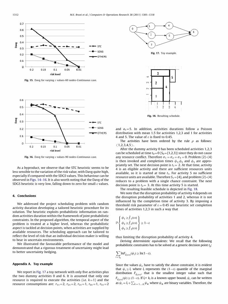
Fig. 15. Davg for varying e values-60 nodes-Continuous case.
Fig. 16. Davg for varying e values-90 nodes-Continuous case.
Fig. 18. Resulting schedule.
Fig. 17. Toy example.
M.E. Bruni et al. / Computers & Operations Research 38 (2011) 1305–13181312
As a byproduct, we observe that the STC heuristic seems to beless sensible to the variation of the risk value, with Davg quite high,especially if compared with the SDGS values. This behaviour can beobserved in Figs. 14–16. It is also worth noting that the Davg of theSDGS heuristic is very low, falling down to zero for small e values.
4. Conclusions
We addressed the project scheduling problem with randomactivity duration developing a tailored heuristic procedure for itssolution. The heuristic exploits probabilistic information on ran-dom activities duration within the framework of joint probabilisticconstraints. In the proposed algorithm, the temporal aspect of theproblem is treated at a higher level, whereas the probabilisticaspect is tackled at decision points, when activities are supplied byavailable resources. The scheduling approach can be tailored toreflect the level of risk that an individual decision maker is willingto bear in uncertain environments.
We illustrated the favourable performance of the model anddemonstrated that a rigorous treatment of uncertainty might leadto better uncertainty hedging.
Appendix A. Toy example
We report in Fig. 17 a toy network with only five activities plusthe two dummy activities 0 and 6. It is assumed that only oneresource is required to execute the activities (i.e. k¼1) and theresource consumptions are: r11¼2, r21¼2, r31¼1, r41¼1, r51¼2
and a1¼5. In addition, activities durations follow a Poissondistribution with mean 1.5 for activities 1,2,3 and 1 for activities4 and 5. The value of e is fixed to 0.45.
The activities have been ordered by the rule r as follows:/1,2,3,4,5S.
After the dummy activity 0 has been scheduled activities 1,2,3can be scheduled at time t0¼0 (S0¼{1,2,3}) since they do not causeany resource conflict. Therefore s1 ¼ s2 ¼ s3 ¼ 0. Problem (2)–(4)is then invoked and completion times f1,f2 and f3 are appro-priately set. The next decision point is t1¼ 2. At that time, activity4 is an eligible activity and there are sufficient resources unitsavailable, so it is started at time t1. For activity 5 no sufficientresource units are available. Therefore S1¼{4}, and problem (2)–(4)reduces to a problem with a single chance constraint. The nextdecision point is t2¼ 3. At this time activity 5 is started.
The resulting feasible schedule is depicted in Fig. 18.We note that the disruption probability of activity 4 depends on
the disruption probability of activities 1 and 2, whereas it is notinfluenced by the completion time of activity 3. By imposing athreshold risk parameter of e¼ 0:45 our heuristic set completiontimes of activities 1,2,3 in such a way that
P
f1Z f 1ðoÞf2Z f 2ðoÞf3Z f 3ðoÞ
8>><>>:
9>>=>>;Z1�e
thus limiting the disruption probability of activity 4.Deriving deterministic equivalents: We recall that the following
probabilistic constraints has to be solved at a generic decision point tg:
XiASg
lnFdiðoÞðciÞZ lnð1�eÞ:
Since the values ci, have to satisfy the above constraint, it is evidentthat ciZ li where li represents the ð1�eÞ quantile of the marginaldistribution F
diðoÞ, that is the smallest integer value such that
FdiðoÞðcÞZ ð1�eÞ. If li+ ki is a known upper bound, ci can be written
as ci ¼ liþP
k ¼ 1,...,kicik where cik are binary variables. Therefore, the

M.E. Bruni et al. / Computers & Operations Research 38 (2011) 1305–1318 1313
probabilistic constraints can be rewritten asXiA Sg
Xk ¼ 1,...,ki
aikcikZp
where aik ¼ lnFdiðoÞðliþkÞ�lnF
diðoÞðliþk�1Þ and p¼ lnð1�eÞ�lnFðlÞ.
For the toy example presented above the vectorsf1,f2 and f3 can berewritten as
c1 ¼ l1þXk1
k ¼ 1
c1k ¼ 1þc11þc12þc13þc14þc15
c2 ¼ l2þXk2
k ¼ 1
c1k ¼ 1þc21þc22þc23þc24þc25
and
c3 ¼ l3þXk3
k ¼ 1
c2k ¼ 1þc31þc32þc33þc34þc35
Therefore, the joint probabilistic constraints can be transformedin the following mixed integer problem.
min Mpar
Mpar Z1þþc11þc12þc13þc14þc15
Mpar Z1þc21þc22þc23þc24þc25
Mpar Z1þc31þc32þc33þc34þc35
a11c11þa12c12þa13c13þa14c14þa15c15þa21c21
Table 1Results on 30 nodes test problems-discrete case.
ð1�eÞ ¼ 0:8 ð1�eÞ ¼ 0:85 ð1�e
Tavg TPCP Davg Mak Tavg TPCP Davg Mak Tavg
1. PSGS-MaxC 52.12 0.17 0.57 84 37.89 0.20 0.49 91 26.55
2. PSGS-MinC 53.04 0.15 0.56 97 36.47 0.20 0.48 103 22.49
3. PSGS-MaxDnC 58.04 0.14 0.58 94 38.73 0.19 0.49 96 28.11
4. PSGS-MinD 51.37 0.15 0.56 91 37.89 0.23 0.49 97 24.38
5. SSGS-MaxC 53.38 0.16 0.56 93 37.19 0.25 0.48 99 25.82
6. SSGS-MinC 57.19 0.15 0.58 99 37.85 0.23 0.48 106 25.80
7. SSGS-MaxDnC 50.39 0.17 0.55 95 37.13 0.25 0.47 102 25.20
8. SSGS-MinD 53.63 0.17 0.56 99 38.42 0.23 0.48 104 25.10
9. PSGS-LST 52.10 0.14 0.57 84 35.51 0.24 0.48 90 23.38
10. PSG-LFT 50.62 0.15 0.57 84 36.45 0.22 0.49 90 23.78
11. PSGS-MTS 50.37 0.14 0.57 86 38.16 0.18 0.51 90 24.18
A. SDGS-MaxC 29.94 0.46 0.26 93 17.32 0.59 0.21 101 12.23
B. SDGS-MinC 32.33 0.28 0.30 96 28.58 0.32 0.29 108 17.80
C. SDGS-MaxDnC 27.68 0.44 0.27 99 22.37 0.45 0.22 103 12.52
D. SDGS-MinD 26.30 0.35 0.30 100 24.25 0.27 0.23 105 12.87
STC 31.33 0.6 0.45 96 21.45 0.74 0.4 104 17.38
RFDFF 93.43 0.021 0.95 97 93.06 0.02 0.95 104 93.06
Table 2Results on 60 nodes test problems-discrete case.
ð1�eÞ ¼ 0:8 ð1�eÞ ¼ 0:85 ð1�eÞ ¼
Tavg TPCP Davg Mak Tavg TPCP Davg Mak Tavg
1. PSGS-MaxC 170.64 0.01 0.69 116 126.35 0.02 0.69 122 73.51
2. PSGS-MinC 154.63 0.01 0.65 121 114.36 0.03 0.66 130 73.05
3. PSGS-
MaxDnC
165.49 0.01 0.67 119 127.90 0.03 0.69 124 79.37
4. PSGS-MinD 156.20 0.01 0.66 121 120.15 0.04 0.68 129 71.62
þa22c22þa23c23þa24c24þa25c25
þa31c31þa32c32þa33c33þa34c34þa35c35
Z lnð1�eÞ�lnðð1�eÞ3Þ
c11,c12,c13,c14,c15,c21,c22,c23,c24,c25,c31,c32,
c33,c34,c35Af0,1gMpar Z0
where c1,c2 and c3 are defined as above.If we instead suppose that d1ðoÞ, d2ðoÞ and d3ðoÞ follow a
Uniform distribution U1[a1,b1], U2[a2,b2] and U3[a3,b3], respectively,the joint probabilistic constraints can be transformed in the followingnonlinear problem.
min Mpar
Mpar Zf1
Mpar Zf2
Mpar Zf3
lnFd1ðoÞðf1Þþ lnF ^d2ðoÞ
ðf2Þþ lnFd3ðoÞðf3ÞZ lnð1�eÞ or equivalently
lnf1�a1
b1�a1
� �þ ln
f2�a2
b2�a2
� �þ ln
f3�a3
b3�a3
� �Z lnð1�eÞ
f1,f2,f3,Mpar Z0
Appendix B. Computational results
Þ ¼ 0:9 ð1�eÞ ¼ 0:95 ð1�eÞ ¼ 0:99
TPCP Davg Mak Tavg TPCP Davg Mak Tavg TPCP Davg Mak
0.30 0.39 95 9.78 0.68 0.18 110 1.69 0.93 0.04 133
0.36 0.35 112 8.98 0.63 0.17 126 1.66 0.91 0.04 151
0.30 0.41 104 10.07 0.62 0.19 120 1.73 0.91 0.04 143
0.35 0.38 105 8.80 0.68 0.17 116 1.69 0.92 0.04 139
0.36 0.37 105 10.74 0.62 0.19 119 1.65 0.94 0.04 144
0.33 0.38 113 10.96 0.59 0.19 128 1.90 0.91 0.04 154
0.35 0.37 109 9.09 0.67 0.16 123 1.87 0.91 0.04 146
0.37 0.37 113 10.00 0.64 0.18 130 1.72 0.92 0.04 155
0.30 0.37 96 9.80 0.59 0.19 109 1.64 0.91 0.04 131
0.33 0.37 97 9.56 0.65 0.18 113 1.52 0.94 0.03 132
0.28 0.38 97 9.30 0.62 0.18 113 1.61 0.92 0.04 132
0.58 0.19 107 5.09 0.86 0.09 123 1.11 0.95 0.02 143
0.41 0.29 116 5.45 0.81 0.10 133 1.23 0.95 0.03 157
0.64 0.21 111 4.93 0.81 0.10 125 1.10 0.96 0.02 148
0.52 0.20 112 5.31 0.82 0.10 128 1.00 0.95 0.02 150
0.81 0.35 111 12.57 0.9 0.25 127 10.02 0.94 0.2 149
0.02 0.95 110 93.06 0.02 0.95 126 93.06 0.02 0.95 148
0:9 ð1�eÞ ¼ 0:95 ð1�eÞ ¼ 0:99
TPCP Davg Mak Tavg TPCP Davg Mak Tavg TPCP Davg Mak
0.12 0.55 133 33.38 0.43 0.32 150 5.80 0.85 0.07 177
0.14 0.53 140 29.63 0.45 0.28 156 5.76 0.87 0.07 188
0.12 0.56 135 35.35 0.38 0.33 152 5.92 0.84 0.07 183
0.15 0.53 139 31.39 0.43 0.29 155 5.35 0.87 0.06 186

Table 3Results on 90 nodes test problems-discrete case.
ð1�eÞ ¼ 0:8 ð1�eÞ ¼ 0:85 ð1�eÞ ¼ 0:9 ð1�eÞ ¼ 0:95 ð1�eÞ ¼ 0:99
Tavg TPCP Davg Mak Tavg TPCP Davg Mak Tavg TPCP Davg Mak Tavg TPCP Davg Mak Tavg TPCP Davg Mak
1. PSGS-MaxC 230.66 0.01 0.76 132 168.46 0.03 0.69 137 109.87 0.08 0.59 156 45.65 0.43 0.07 175 8.67 0.81 0.07 211
2. PSGS-MinC 214.99 0.01 0.73 140 136.39 0.05 0.63 149 95.61 0.13 0.52 161 36.99 0.49 0.05 181 6.32 0.89 0.05 215
3. PSGS-MaxDnC 229.88 0.00 0.75 129 164.57 0.01 0.68 144 105.68 0.13 0.56 156 48.45 0.33 0.06 173 7.56 0.85 0.06 206
4. PSGS-MinD 220.02 0.02 0.74 148 167.17 0.03 0.68 155 102.03 0.11 0.54 170 39.19 0.50 0.06 195 7.80 0.84 0.06 234
5. SSGS-MaxC 189.75 0.02 0.68 133 139.11 0.08 0.60 145 90.91 0.24 0.48 156 42.74 0.43 0.05 171 6.56 0.88 0.05 208
6. SSGS-MinD 185.08 0.03 0.67 146 126.16 0.09 0.89 153 78.73 0.25 0.40 164 34.54 0.51 0.04 184 5.88 0.89 0.04 220
7. SSGS-MaxDnC 214.04 0.02 0.71 130 137.69 0.05 0.59 139 88.15 0.21 0.46 148 41.79 0.40 0.05 168 6.40 0.87 0.05 202
8. SSGS-MinD 185.53 0.05 0.67 161 135.60 0.11 0.59 172 80.80 0.26 0.44 185 35.16 0.54 0.05 206 6.42 0.88 0.05 247
9. PSGS-LST 233.56 0.00 0.75 111 163.91 0.00 0.67 125 109.96 0.05 0.57 130 48.51 0.32 0.08 160 9.46 0.82 0.08 184
10. PSGS-LFT 240.92 0.00 0.75 113 165.54 0.01 0.68 120 112.37 0.05 0.57 132 46.11 0.35 0.07 156 8.10 0.83 0.07 186
11. PSGS-MTS 230.54 0.01 0.75 134 167.19 0.02 0.69 142 113.92 0.10 0.58 156 49.54 0.32 0.07 183 8.21 0.84 0.07 210
A. SDGS-MaxC 19.06 0.56 0.09 201 13.15 0.60 0.07 215 7.34 0.78 0.04 224 3.59 0.87 0.00 259 0.59 0.98 0.00 289
B. SDGS-MinC 21.30 0.48 0.10 206 12.93 0.65 0.07 218 9.57 0.78 0.06 237 2.92 0.87 0.00 266 0.64 0.97 0.00 283
C. SDGS-MaxDnC 19.96 0.55 0.10 194 16.36 0.61 0.08 212 7.87 0.78 0.05 212 3.63 0.89 0.01 247 0.75 0.97 0.01 288
D. SDGS-MinD 20.11 0.56 0.10 193 15.34 0.61 0.08 203 8.35 0.74 0.05 217 3.29 0.90 0.01 245 0.71 0.97 0.01 288
STC 450.80 0.35 0.94 201 245.49 0.65 0.82 215 144.25 0.88 0.70 224 79.78 0.96 0.54 259 55.84 0.99 0.44 289
RFDFF 584.95 0.39 0.983 201 584.95 0.39 0.983 215 584.95 0.39 0.983 224 584.95 0.39 0.983 259 584.95 0.39 0.983 289
Table 2 (continued )
ð1�eÞ ¼ 0:8 ð1�eÞ ¼ 0:85 ð1�eÞ ¼ 0:9 ð1�eÞ ¼ 0:95 ð1�eÞ ¼ 0:99
Tavg TPCP Davg Mak Tavg TPCP Davg Mak Tavg TPCP Davg Mak Tavg TPCP Davg Mak Tavg TPCP Davg Mak
5. SSGS-MaxC 150.72 0.02 0.62 122 107.25 0.09 0.61 129 71.33 0.18 0.49 140 31.10 0.46 0.28 156 5.24 0.88 0.06 186
6. PSGS-MinC 155.62 0.02 0.63 132 114.95 0.07 0.64 141 69.17 0.20 0.49 153 30.46 0.48 0.26 173 5.06 0.88 0.06 206
7. PSGS-
MaxDnC
148.88 0.03 0.63 125 111.81 0.08 0.62 132 68.06 0.15 0.49 142 29.77 0.49 0.27 160 5.50 0.87 0.06 190
8. PSGS-MinD 141.47 0.04 0.62 132 107.49 0.08 0.61 140 67.81 0.20 0.48 151 28.03 0.51 0.25 170 5.63 0.87 0.06 204
9. PSGS-LST 161.14 0.01 0.74 111 120.34 0.02 0.68 119 77.18 0.08 0.57 129 32.02 0.47 0.31 144 6.33 0.84 0.07 173
10. PSGS-LFT 160.62 0.01 0.74 111 118.85 0.02 0.68 118 76.95 0.08 0.57 123 31.87 0.41 0.30 147 6.11 0.83 0.07 172
11. PSGS-MST 160.01 0.00 0.74 110 119.13 0.03 0.68 118 72.05 0.09 0.55 126 30.96 0.35 0.30 142 5.46 0.86 0.07 170
A. SDGS-MaxC 32.64 0.40 0.18 146 26.79 0.47 0.15 159 22.18 0.62 0.11 170 21.25 0.84 0.15 190 20.20 0.97 0.13 234
B. SDGS-MinC 33.96 0.41 0.20 152 27.08 0.46 0.20 163 26.65 0.62 0.20 177 21.02 0.81 0.19 188 19.52 0.96 0.13 233
C. SDGS-
MaxDnC
27.02 0.40 0.17 151 22.45 0.57 0.18 157 21.80 0.63 0.12 172 18.82 0.80 0.14 188 16.53 0.97 0.12 233
D. SDGS-MinD 22.86 0.38 0.15 149 21.97 0.56 0.16 155 21.56 0.68 0.12 169 21.50 0.82 0.11 191 16.72 0.97 0.12 225
STC 76.34 0.72 0.6 148 51.51 0.83 0.48 157 39.17 0.91 0.43 175 25.55 0.96 0.35 191 21.11 0.99 0.31 233
RFDFF 163.196 0.06 0.86 149 163.196 0.06 0.86 159 163.196 0.06 0.86 175 163.196 0.06 0.86 190 163.196 0.06 0.86 233
Table 4Results on 30 nodes test problems-continuous case.
ð1�eÞ ¼ 0:8 ð1�eÞ ¼ 0:85 ð1�eÞ ¼ 0:9 ð1�eÞ ¼ 0:95 ð1�eÞ ¼ 0:99
Tavg TPCP Davg Mak Tavg TPCP Davg Mak Tavg TPCP Davg Mak Tavg TPCP Davg Mak Tavg TPCP Davg Mak
1. PSGS-MaxC 27.99 0.27 0.43 119 14.07 0.44 0.31 125 7.11 0.59 0.21 132 2.59 0.84 0.08 136 0.00 1.00 0.00 139
2. PSGS-MinC 27.74 0.26 0.43 133 13.54 0.45 0.30 139 7.57 0.62 0.22 144 2.65 0.84 0.08 149 0.00 1.00 0.00 154
3. PSGS-MaxDnC 32.14 0.23 0.48 129 17.12 0.36 0.37 135 8.20 0.56 0.23 141 2.51 0.85 0.08 146 0.00 1.00 0.00 151
4. PSGS-MinD 26.57 0.28 0.41 128 13.99 0.41 0.31 133 6.81 0.60 0.20 138 2.34 0.85 0.07 143 0.00 1.00 0.00 148
5. SSGS-MaxC 30.39 0.25 0.45 128 14.96 0.41 0.32 134 7.18 0.60 0.21 139 2.40 0.84 0.08 144 0.00 1.00 0.00 149
6. SSGS-MinC 30.42 0.25 0.45 141 13.96 0.44 0.31 147 8.05 0.58 0.23 152 2.45 0.84 0.08 156 0.00 1.00 0.00 163
7. SSGS-MaxDnC 29.93 0.25 0.46 132 15.60 0.38 0.34 137 8.52 0.52 0.24 142 2.18 0.86 0.07 149 0.00 1.00 0.00 152
8. SSGS-MinD 28.82 0.25 0.43 140 14.28 0.41 0.31 145 8.06 0.56 0.23 150 2.38 0.86 0.08 156 0.00 1.00 0.00 160
9. PSGS-LST 27.32 0.24 0.43 118 14.58 0.38 0.32 123 7.34 0.59 0.21 128 2.22 0.88 0.07 133 0.00 1.00 0.00 137
10. PSGS-LFT 26.22 0.29 0.42 118 14.20 0.42 0.32 123 7.56 0.58 0.22 128 2.30 0.88 0.07 132 0.00 1.00 0.00 137
11. PSGS-MTS 27.59 0.26 0.44 118 14.57 0.38 0.32 123 7.39 0.60 0.21 128 2.40 0.82 0.08 133 0.00 1.00 0.00 147
M.E. Bruni et al. / Computers & Operations Research 38 (2011) 1305–13181314

Table 5Results on 60 nodes test problems-continuous case.
ð1�eÞ ¼ 0:8 ð1�eÞ ¼ 0:85 ð1�eÞ ¼ 0:9 ð1�eÞ ¼ 0:95 ð1�eÞ ¼ 0:99
Tavg TPCP Davg Mak Tavg TPCP Davg Mak Tavg TPCP Davg Mak Tavg TPCP Davg Mak Tavg TPCP Davg Mak
1. PSGS-MaxC 96.71 0.04 0.63 167 53.55 0.18 0.51 176 25.82 0.40 0.35 183 8.29 0.69 0.13 188 0.00 1.00 0.00 197
2. PSGS-MinC 95.43 0.03 0.62 178 49.51 0.20 0.47 186 23.00 0.40 0.31 193 7.12 0.73 0.11 200 0.00 1.00 0.00 205
3. PSGS-
MaxDnC
103.35 0.05 0.65 174 52.45 0.16 0.50 180 24.25 0.38 0.33 191 8.44 0.74 0.13 193 0.00 1.00 0.00 196
4. PSGS-MinD 85.00 0.08 0.59 175 49.61 0.20 0.47 183 26.21 0.40 0.35 188 8.02 0.73 0.12 197 0.00 1.00 0.00 204
5. SSGS-MaxC 96.06 0.06 0.61 174 47.36 0.22 0.45 184 22.02 0.43 0.30 191 7.82 0.75 0.12 197 0.00 1.00 0.00 204
6. SSGS-MinC 94.35 0.06 0.60 190 47.20 0.21 0.44 201 23.62 0.41 0.32 208 7.22 0.76 0.11 216 0.00 1.00 0.00 222
7. SSGS-
MaxDnC
96.90 0.07 0.63 178 50.21 0.19 0.48 186 23.53 0.42 0.32 193 7.71 0.75 0.12 202 0.00 1.00 0.00 208
8. SSGS-MinD 92.49 0.07 0.59 191 46.32 0.21 0.45 199 24.69 0.43 0.33 208 6.47 0.78 0.10 216 0.00 1.00 0.00 222
9. PSGS-LST 90.56 0.05 0.63 154 49.72 0.19 0.48 161 25.17 0.33 0.35 168 7.91 0.72 0.12 174 0.00 1.00 0.00 179
10. PSSG-LFT 91.61 0.05 0.63 153 50.91 0.17 0.49 161 24.31 0.38 0.34 168 7.56 0.71 0.12 172 0.00 1.00 0.00 178
11. PSGS-MTS 87.77 0.04 0.61 164 50.97 0.17 0.49 173 24.51 0.39 0.34 179 8.17 0.75 0.13 185 0.00 1.00 0.00 192
A. SDGS-MaxC 25.53 0.96 0.05 180 13.77 0.97 0.04 185 5.81 0.99 0.01 200 1.38 1.00 0.01 206 0.00 1.00 0.00 230
B. SDGS-MinC 27.67 0.95 0.24 182 14.18 0.96 0.15 193 6.54 0.98 0.09 204 1.90 0.99 0.03 216 0.00 1.00 0.00 240
C. SDGS-
MaxDnC
50.76 0.85 0.27 179 13.51 0.96 0.16 189 6.56 0.98 0.10 200 1.49 0.99 0.02 206 0.00 1.00 0.00 234
D. SDGS-MinD 50.52 0.86 0.25 179 16.15 0.95 0.18 180 5.66 0.97 0.09 194 2.35 0.99 0.04 210 0.00 1.00 0.00 215
STC 18.04 0.98 0.32 180 19.95 0.99 0.35 188 18.03 0.99 0.33 200 19.63 0.99 0.33 207 17.63 0.99 0.32 233
RFDFF 170.747 0.06 0.96 178 170.747 0.06 0.96 187 170.747 0.06 0.96 201 170.747 0.06 0.96 209 170.747 0.06 0.96 235
Table 6Results on 90 nodes test problems-continuous case.
ð1�eÞ ¼ 0:8 ð1�eÞ ¼ 0:85 ð1�eÞ ¼ 0:9 ð1�eÞ ¼ 0:95 ð1�eÞ ¼ 0:99
Tavg TPCP Davg Mak Tavg TPCP Davg Mak Tavg TPCP Davg Mak Tavg TPCP Davg Mak Tavg TPCP Davg Mak
1. PSGS-MaxC 121.68 0.13 0.58 171 68.47 0.20 0.44 178 34.34 0.37 0.32 185 13.66 0.99 0.00 191 0.00 1.00 0.00 196
2. PSGS-MinC 110.39 0.15 0.54 181 54.15 0.32 0.37 189 26.15 0.48 0.25 195 10.31 0.99 0.00 203 0.00 1.00 0.00 211
3. PSGS-MaxDnC 120.86 0.13 0.56 172 69.09 0.24 0.44 180 30.92 0.43 0.29 188 11.62 0.99 0.00 198 0.00 1.00 0.00 200
4. PSGS-MinD 116.91 0.15 0.50 175 67.83 0.27 0.43 184 31.09 0.43 0.29 194 12.65 0.99 0.00 194 0.00 1.00 0.00 201
5. SSGS-MaxC 116.51 0.15 0.53 174 58.49 0.29 0.39 181 25.24 0.54 0.24 190 10.92 0.99 0.00 196 0.00 1.00 0.00 203
6. SSGS-MinC 117.52 0.16 0.52 185 56.55 0.25 0.37 193 25.52 0.48 0.24 202 9.19 0.99 0.00 205 0.00 1.00 0.00 214
7. SSGS-MaxDnC 119.89 0.17 0.55 177 56.89 0.30 0.38 185 25.15 0.52 0.24 194 9.58 0.99 0.00 200 0.00 1.00 0.00 207
8. SSGS-MinD 109.42 0.19 0.50 190 50.64 0.39 0.35 195 25.43 0.51 0.24 204 9.94 0.99 0.00 212 0.00 1.00 0.00 217
9. PSGS-LST 125.53 0.12 0.58 152 70.10 0.19 0.45 158 30.97 0.40 0.29 165 11.37 0.99 0.00 171 0.00 1.00 0.00 177
10. PSGS-LFT 126.87 0.12 0.58 153 68.27 0.28 0.44 160 30.73 0.44 1.27 166 13.33 0.99 0.00 174 0.00 1.00 0.00 178
11. PSGS-MTS 129.23 0.12 0.52 168 68.12 0.28 1.27 174 31.11 0.39 0.54 182 12.60 0.99 0.00 187 0.00 1.00 0.00 193
A. SDGS-MaxC 14.20 0.65 0.10 207 5.38 0.80 0.05 224 1.55 0.89 0.02 245 0.61 1.00 0.00 246 0.00 1.00 0.00 254
B. SDGS-MinC 12.89 0.59 0.08 223 5.95 0.77 0.05 230 2.41 0.83 0.03 244 0.64 1.00 0.00 254 0.00 1.00 0.00 264
C. SDGS-MaxDnC 12.30 0.60 0.08 225 5.18 0.79 0.04 228 2.11 0.89 0.02 243 0.76 1.00 0.00 248 0.00 1.00 0.00 260
D. SDGS-MinD 12.31 0.62 0.08 217 6.17 0.74 0.04 227 2.50 0.88 0.03 233 0.67 1.00 0.00 245 0.00 1.00 0.00 264
STC 75.53 0.95 0.52 218 76.57 0.93 0.54 227 70.5 0.95 0.50 241 63.1 0.95 0.48 248 58.34 0.97 0.44 258
RFDFF 230.36 0.11 0.71 218 230.36 0.11 0.71 227 230.36 0.11 0.71 241 230.36 0.11 0.71 248 230.36 0.11 0.71 258
Table 4 (continued )
ð1�eÞ ¼ 0:8 ð1�eÞ ¼ 0:85 ð1�eÞ ¼ 0:9 ð1�eÞ ¼ 0:95 ð1�eÞ ¼ 0:99
Tavg TPCP Davg Mak Tavg TPCP Davg Mak Tavg TPCP Davg Mak Tavg TPCP Davg Mak Tavg TPCP Davg Mak
A. SDGS-MaxC 12.09 0.85 0.19 139 3.26 0.90 0.08 152 1.66 0.94 0.05 159 0.55 0.97 0.02 161 0.00 1.00 0.00 172
B. SDGS-MinC 26.92 0.69 0.40 130 14.70 0.74 0.28 136 7.30 0.85 0.18 142 1.77 0.94 0.05 152 0.00 1.00 0.00 165
C. SDGS-MaxDnC 22.31 0.71 0.33 120 9.90 0.83 0.22 129 5.77 0.88 0.15 133 1.58 0.95 0.04 142 0.00 1.00 0.00 153
D. SDGS-MinD 28.00 0.64 0.39 125 15.57 0.77 0.29 130 6.41 0.87 0.16 136 1.73 0.93 0.05 146 0.00 1.00 0.00 158
STC 11.13 0.97 0.33 128 10.15 0.98 0.32 126 10.80 0.99 0.34 140 9.64 0.98 0.30 150 9.02 0.99 0.29 160
RFDFF 89.27 0.011 0.95 129 89.27 0.011 0.95 137 89.27 0.011 0.95 141 89.27 0.011 0.95 150 89.27 0.011 0.95 161
M.E. Bruni et al. / Computers & Operations Research 38 (2011) 1305–1318 1315

Table 7Average, minimum and maximum number of variables and constraints per iteration.
e 0.2 0.15 0.1
Number of variables Number of
constraints
It Number of
variables
Number of
constraints
It Number of
variables
Number of
constraints
It
max min avg max min avg avg max min avg max min avg avg max min avg max min avg avg
30
A
Discrete 16.71 9.38 12.41 8.25 5.00 5.65 7.63 16.29 9.00 11.49 8.50 5.00 5.75 7.88 15.57 8.13 10.63 8.50 5.00 5.90 7.75
Continuous 3.78 2.00 2.45 4.78 3.00 3.45 11.22 4.00 2.00 2.60 5.00 3.00 3.60 9.90 3.90 2.00 2.50 4.90 3.00 3.50 9.70
B
Discrete 16.14 9.25 12.79 8.50 5.00 6.04 4.63 15.50 9.00 11.34 8.50 5.00 5.87 5.38 15.00 7.63 10.42 8.75 5.00 5.99 5.88
Continuous 4.00 2.00 2.39 5.00 3.00 3.39 8.22 4.00 2.00 2.45 5.00 3.00 3.45 8.49 3.99 2.00 2.49 4.99 3.00 3.49 7.77
Discrete 16.50 9.00 12.43 8.25 5.00 5.66 8.00 16.00 8.50 11.98 8.50 5.00 6.04 7.25 14.57 7.75 10.63 8.50 5.00 5.96 7.63
Continuous 3.89 2.00 2.45 4.89 3.00 3.45 9.33 3.90 2.00 2.43 4.90 3.00 3.43 9.85 3.90 2.00 2.48 4.90 3.00 3.48 8.98
D
Discrete 17.14 8.75 12.84 8.25 5.00 5.90 8.00 16.38 8.63 11.36 8.50 5.00 5.76 7.50 14.43 7.38 9.97 8.50 5.00 5.62 8.63
Continuous 4.22 2.00 2.47 5.22 3.00 3.47 9.22 4.19 2.00 2.50 5.19 3.00 3.50 8.48 4.09 2.00 2.57 5.09 3.00 3.57 8.40
60
A
Discrete 23.70 8.90 15.30 9.80 5.00 6.73 18.70 23.60 8.50 13.99 10.60 5.00 6.73 18.40 19.89 7.11 11.77 10.78 5.00 6.54 17.22
Continuous 5.40 2.00 3.34 6.40 3.00 4.34 16.10 5.20 2.10 3.31 6.20 3.10 4.31 16.30 5.20 2.00 3.13 6.20 3.00 4.13 16.80
B
Discrete 24.70 9.10 15.17 10.00 5.00 6.68 17.80 23.00 8.40 13.41 10.20 5.00 6.49 17.70 19.11 7.44 11.55 10.11 5.00 6.45 17.22
Continuous 4.90 2.00 3.19 5.90 3.00 4.19 16.00 4.80 2.00 3.14 5.80 3.00 4.14 16.20 5.00 2.00 3.08 6.00 3.00 4.08 16.20
C
Discrete 25.10 8.90 15.67 10.40 5.00 6.92 18.30 22.90 8.30 13.97 10.00 5.00 6.78 18.50 19.56 7.44 12.34 10.11 5.00 6.80 18.44
Continuous 5.40 2.00 3.24 6.40 3.00 4.24 16.50 5.20 2.00 3.32 6.20 3.00 4.32 16.50 4.90 2.00 3.17 5.90 3.00 4.17 16.50
D
Discrete 25.40 8.70 15.73 10.40 5.00 6.91 17.70 23.90 8.40 14.05 10.20 5.00 6.76 19.20 19.00 7.11 12.13 9.89 5.00 6.70 18.56
Continuous 5.10 2.00 3.43 6.10 3.00 4.43 15.10 5.12 2.00 3.25 6.12 3.00 4.25 17.15 4.99 2.10 3.26 5.99 3.10 4.26 16.25
90
A
Discrete 40.67 8.67 20.66 16.33 5.00 8.83 22.00 36.11 9.78 18.74 15.89 5.22 8.82 21.33 32.67 7.89 15.81 16.11 5.00 8.51 22.56
Continuous 7.60 2.00 3.80 8.60 3.00 4.80 21.00 8.60 2.00 4.23 9.60 3.00 5.23 20.50 8.80 2.20 4.52 9.80 3.20 5.52 18.90
B
Discrete 38.60 10.70 20.99 14.80 5.00 8.92 21.30 31.56 8.67 17.75 13.67 5.00 8.34 23.44 27.56 7.78 15.13 14.11 5.00 8.18 23.00
Continuous 8.00 2.00 3.84 9.00 3.00 4.84 20.70 8.00 2.00 4.23 9.00 3.00 5.23 19.90 7.90 2.10 4.54 8.90 3.10 5.54 18.50
C
Discrete 38.33 9.22 21.69 14.78 5.00 9.23 20.44 33.33 9.44 18.67 14.78 5.00 8.74 21.89 30.11 8.22 16.25 15.22 5.00 8.75 21.67
Continuous 8.00 2.00 4.04 9.00 3.00 5.04 21.00 7.80 2.00 4.53 8.80 3.00 5.53 19.20 7.90 2.00 4.75 8.90 3.00 5.75 18.20
D
Discrete 37.44 9.67 21.01 15.22 5.00 8.97 21.56 33.22 9.00 18.91 15.00 5.00 8.84 21.89 29.56 8.11 16.38 15.00 5.00 8.78 21.78
Continuous 7.60 2.00 4.19 8.60 3.00 5.19 19.70 8.30 2.20 4.66 9.30 3.20 5.66 18.60 8.00 2.00 4.58 9.00 3.00 5.58 19.30
e 0.05 0.01
Number of variables Number of constraints It Number of variables Number of constraints It
max min avg max min avg avg max min avg max min avg avg
30
A
Discrete 10.86 5.75 7.69 8.25 5.00 5.73 7.38 4.63 3.00 3.34 7.25 4.00 4.68 7.13
Continuous 3.90 2.00 2.52 4.90 3.00 3.52 9.90 4.00 2.10 2.57 5.00 3.10 3.57 8.60
B
Discrete 10.71 5.75 7.93 8.75 5.00 6.03 5.13 4.63 3.00 3.51 7.25 4.00 5.03 4.63
Continuous 3.99 2.00 2.47 4.99 3.00 3.47 8.49 3.80 2.01 2.44 4.80 3.01 3.44 7.86
Discrete 8.49 3.88 5.15 6.72 4.00 4.69 7.72 4.63 3.00 3.49 7.25 4.00 4.98 5.50
Continuous 3.90 2.00 2.47 4.90 3.00 3.47 8.55 3.78 2.00 2.46 4.78 3.00 3.46 8.09
D
Discrete 11.00 5.75 7.67 8.25 5.00 5.73 6.88 4.63 3.00 3.46 7.25 4.00 4.91 5.75
Continuous 3.99 2.00 2.54 4.99 3.00 3.54 8.35 3.98 2.00 2.50 4.98 3.00 3.50 8.61
60
A
Discrete 14.78 5.11 8.77 10.56 5.00 6.47 16.33 5.22 3.00 3.62 8.44 4.00 5.25 17.89
Continuous 5.00 2.00 3.16 6.00 3.00 4.16 16.70 5.30 2.10 3.18 6.30 3.10 4.18 17.40
M.E. Bruni et al. / Computers & Operations Research 38 (2011) 1305–13181316
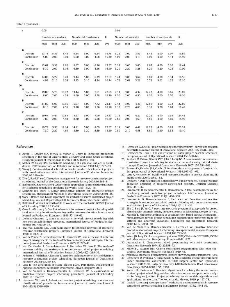
Table 7 (continued )
e 0.05 0.01
Number of variables Number of constraints It Number of variables Number of constraints It
max min avg max min avg avg max min avg max min avg avg
B
Discrete 13.78 5.33 8.45 9.44 5.00 6.24 16.78 5.22 3.00 3.53 8.44 4.00 5.07 16.89
Continuous 5.00 2.00 3.08 6.00 3.00 4.08 15.40 5.00 2.00 3.13 6.00 3.00 4.13 15.90
C
Discrete 13.67 5.33 8.62 9.67 5.00 6.36 17.67 5.33 3.00 3.60 8.67 4.00 5.20 18.44
Continuous 5.30 2.00 3.16 6.30 3.00 4.16 16.40 5.20 2.20 3.28 6.20 3.20 4.28 17.00
D
Discrete 14.00 5.22 8.70 9.44 5.00 6.39 17.67 5.44 3.00 3.67 8.89 4.00 5.34 16.56
Continuous 4.93 2.10 3.24 5.93 3.10 4.24 16.74 4.72 2.02 3.22 5.72 3.02 4.22 17.10
90
A
Discrete 19.89 5.78 10.82 13.44 5.00 7.91 22.89 7.11 3.00 4.32 12.22 4.00 6.65 23.89
Continuous 8.60 2.00 4.58 9.60 3.00 5.58 19.10 8.50 2.00 4.50 9.50 3.00 5.50 19.30
B
Discrete 21.89 5.00 10.55 15.67 5.00 7.72 24.11 7.44 3.00 4.36 12.89 4.00 6.72 22.89
Continuous 8.10 2.00 4.56 9.10 3.00 5.56 18.70 8.10 2.20 4.63 9.10 3.20 5.63 18.40
C
Discrete 19.67 5.44 10.83 13.67 5.00 7.90 23.33 7.11 3.00 4.27 12.22 4.00 6.55 24.44
Continuous 7.80 2.00 4.58 8.80 3.00 5.58 19.20 7.80 2.00 4.69 8.80 3.00 5.69 18.90
D
Discrete 19.78 5.56 11.14 14.11 5.00 8.09 22.67 7.11 3.00 4.42 12.22 4.00 6.83 23.33
Continuous 7.80 2.20 4.69 8.80 3.20 5.69 18.20 7.80 2.10 4.58 8.80 3.10 5.58 19.10
M.E. Bruni et al. / Computers & Operations Research 38 (2011) 1305–1318 1317
References
[1] Aytug H, Lawley MA, McKay K, Mohan S, Uzsoy R. Executing productionschedules in the face of uncertainties: a review and some future directions.European Journal of Operational Research 2005;161:86–110.
[2] Mehta SV, Uzsoy RM. Predictable scheduling of a job shop subject to break-downs. IEEE Transactions on Robotics and Automation 1998;14(3):365–78.
[3] Wang J. Constraint-based schedule repair for product development projectswith time-limited constraints. International Journal of Production Economics2005;95:399–414.
[4] Zhu G, Bard JF, Yu G. Disruption management for resource-constrained projectscheduling. Journal of the Operational Research Society 2005;56:365–81.
[5] Igelmund G, Radermacher FJ. Algorithmic approaches to preselective strategiesfor stochastic scheduling problems. Networks 1983;13:29–48.
[6] Mohring RH, Stork F. Linear preselective policies for stochastic projectscheduling. Mathematical Methods of Operations Research 2000;52:501–15.
[7] Stork F. Branch-and-bound algorithms for stochastic resource-constrained projectscheduling. Research Report. 702/2000. Technische Universitat, Berlin; 2000.
[8] Ballestin F. When it is worthwhile to work with the stochastic RCPSP? Journalof Scheduling 2007;10:153–66.
[9] Golenko-Ginzburg D, Gonik A. A heuristic for network project scheduling withrandom activity durations depending on the resource allocation. InternationalJournal on Production Economics 1998;55:149–62.
[10] Golenko-Ginzburg D, Gonik A. Stochastic network project scheduling withnon-consumable limited resources. International Journal of Production Eco-nomics 1997;48:29–37.
[11] Tsai YW, Gemmil DD. Using tabu search to schedule activities of stochasticresource-constrained projects. European Journal of Operational Research1998;111:129–41.
[12] Van de Vonder S, Demeulemeester E, Herroelen W, Leus R. The use of buffers inproject management: the trade-off between stability and makespan. Interna-tional Journal of Production Economics 2005;97:227–40.
[13] Van De Vonder S, Demeulemeester E, Herroelen W, Leus R. The trade-offbetween stability and makespan in resource-constrained project scheduling.International Journal of Production Research 2006;44(2):215–36.
[14] Artigues C, Michelon P, Reusser S. Insertion techniques for static and dynamicresource-constrained project scheduling. European Journal of OperationalResearch 2003;149:249–67.
[15] Leus R. The generation of stable project plans. PhD thesis, Department ofApplied Economics, Katholieke Universiteit Leuven, Belgium; 2003.
[16] Van de Vonder S, Demeulemeester E, Herroelen W. A classification ofpredictive-reactive project scheduling procedures. Journal of Scheduling2007;10:195–207.
[17] Herroelen W, Leus R. Robust and reactive project scheduling: a review andclassification of procedures. International Journal of production Research2004;42(8):1599–620.
[18] Herroelen W, Leus R. Project scheduling under uncertainty—survey and researchpotentials. European Journal of Operational Research 2005;165(2):289–306.
[19] Herroelen W, Leus R. The construction of stable project baseline schedules.European Journal of Operational Research 2004;156:550–65.
[20] Rabbani M, Fatemi Ghomi SMT, Jolai F, Lahiji NS. A new heuristic for resource-constrained project scheduling in stochastic networks using critical chainconcept. European Journal of Operational Research 2007;176:794–808.
[21] Tavares LV, Ferreira JAA, Coelho JS. On the optimal management of project risk.European Journal of Operational Research 1998;107:451–69.
[22] Leus R, Herroelen W. Stability and resource allocation in project planning. IIETransactions 2004;36:667–82.
[23] Deblaere F, Demeulemeester E, Herroelen W, Van de Vonder S. Robust resourceallocation decisions in resource-constrained projects. Decision Sciences2007;38:1–37.
[24] Lambrechts O, Demeulemeester E, Herroelen W. A tabu search procedure fordeveloping robust predictive project schedules. International Journal ofProduction Economics 2007;111(2):496–508.
[25] Lambrechts O, Demeulemeester E, Herroelen W. Proactive and reactivestrategies for resource-constrained project scheduling with uncertain resourceavailabilities. Journal of Scheduling 2008;11(2):121–36.
[26] Zhu G, Bard JF, Yu G. A two-stage stochastic programming approach for projectplanning with uncertain activity durations. Journal of Scheduling 2007;10:167–80.
[27] Klerides E, Hadjiconstantinou E. A decomposition-based stochastic program-ming approach for the project scheduling problem under time/cost trade-offsettings and uncertain durations. Computers and Operations Research2010;37(12):2131–40.
[28] Van de Vonder S, Demeulemeester E, Herroelen W. Proactive heuristicprocedures for robust project scheduling: an experimental analysis. EuropeanJournal of Operational Research 2008;189:723–33.
[29] Wiest JD, Levy FK. A management guide to PERT/CPM with GERT/PDM/DCPMand other networks. New Jersey: Prentice-Hall; 1977.
[30] Jagannathan R. Chance-constrained programming with joint constraints.Operations Research 1974;22(2):358–72.
[31] Miller BL, Wagner HM. Chance constrained programming with joint con-straints. Operations Research 1965;13(6):930–45.
[32] Prekopa A. Stochastic programming. Boston: Kluwer Academic Publishers; 1995.[33] Dentcheva D, Prekopa A, Ruszczynski A. On stochastic integer programming
under probabilistic constraints. RUTCOR-Rutgers Center for OperationsResearch RRR 29-98, Rutgers University, 640 Bartholomew Road Piscataway,New Jersey 08854-8003, USA; 1998.
[34] Kolisch R, Hartmann S. Heuristic algorithms for solving the resource-con-strained project scheduling problem: classification and computational analy-sis. In: Weglarz J, editor. Project scheduling: recent models, algorithms andapplications. Amsterdam, The Netherlands: Kluwer; 1999. p. 147–78.
[35] Davis E, Patterson J. A comparison of heuristic and optimum solutions in resourceconstrained project scheduling. Management Science 1975;21:944–55.

M.E. Bruni et al. / Computers & Operations Research 38 (2011) 1305–13181318
[36] Alvarez-Valdes R, Tamarit JM. Heuristic algorithms for resource constrainedproject scheduling. In: Slowinski R, Weglarz J, editors. A review and anempirical analysis. Advances in project scheduling. Amsterdam: Elsevier;1989. p. 113–34.
[37] Bisschop J, Roelofs M. AIMMS. 3.7 User’s guide. Paragon Decision TechnologyB.V., Incline Village, NV, The Netherlands: Optimization, Inc.; 2006.
[38] CPLEX, ILOG CPLEX 6.5: Users Manual, Incline Village, NV: CPLEX Optimization,Inc.; 1999.
[39] Drud A. S. CONOPT: a system for large scale nonlinear optimization. Referencemanual for CONOPT subroutine library, ARKI Consulting and Development A/S,Bagsvaerd, Denmark; 1996.
[40] Kolisch R, Sprecher A. PSPLIB a project scheduling problem library. EuropeanJournal of Operational Research 1997;96:205–16.
[41] Beraldi P, Bruni ME, Guerriero F, Pinto E. Heuristic procedures for the robustproject scheduling problem. Technical Report, ParCoLab, DEIS, University ofCalabria; 2007.