A GRASS-GIS-Based Methodology for

Flash Flood Risk Assessment

in Goa

K. Suprit, Aravind Kalla and V. Vijith

National Institute of Oceanography (CSIR),

Dona Paula, Goa 403004.

6 October 2010

Executive Summary

Recurring floods in Goa cause damage to both property and life.

After the 2 October 2009 flash floods in Canacona Taluka, South Goa,

the Government of Goa constituted a committee (Canacona Flash

Floods Study Committee) to study the flood event and suggest mea-

sures to minimize damages occurring from similar episodes in future.

The committee recommended the developing of a methodology for

flood risk assessment and warning during an intense-rainfall event

which can be implemented elsewhere in Goa with the help of grad-

uate students. This requires the analysis of topography for river flow

(watershed analysis) and converting rainfall to river flow (discharge

calculation). The watershed analysis is based on a free and open

source GIS called GRASS GIS. It calculates the watershed properties

(watershed areas, stream network, slope, etc.). It also identifies and

delineates areas nearest to the stream channel, the ones most likely to

be affected by flash floods (flood-prone areas).

Based on the discharge calculations, a simple method to give warn-

ing of the possible occurrence of flash flood due to intense-rainfall

events is also developed. A simple but widely used hydrological model,

called rational method, is used to calculate the peak discharge in the

selected stream. Based on this method, a flood watch algorithm is

derived, which uses rainfall intensity data from the nearest Automatic

Weather Station (AWS).

The method developed uses free and open software tools and re-

quires a bare minimum of input data, namely, topographic data (Digi-

tal Elevation Model, DEM) and rainfall data, both of which are avail-

able free of cost in the public domain. Its viability is tested for the

flash flood of 2 October 2009 in the Talpona river. The method is

mainly aimed at graduate students of Goa and it is hoped that the

framework will be further strengthened in the future, by incorporat-

ing advanced hydrological flood forecasting models. Thus, this study

aims at being a starting point to have in place a full fledged flash flood

assessment and forecasting system for Goa.

3

1 Introduction

1.1 Background

The west coast of India is one of the maximum rainfall regions of the country,

with ∼ 90% of the rainfall occurs in the monsoon (June–September). The

orography of the coast and heavy rainfall makes the region flood-prone during

intense-rainfall events. These intense-rainfall events occur frequently on the

coast, the probability of these episodes being maximum between latitudinal

band 14◦–16◦ N and near 19◦ N (Francis and Gadgil, 2006).

The state of Goa (Figure 1), (15◦–16◦ N and 73◦–75◦ E) lies in the above

mentioned band of intense rainfall-event-prone area. Overall the climate and

geography of Goa is typical of the west coast of India. The heavy rainfall

experienced here is owing to the presence of Sahyadris. The Sahyadri moun-

tains (also known as the Western Ghats) run along the coast. They rise to a

height of about 1000 m. The peaks of the Sahyadris straddle a very narrow

coastal plain (Figure 1) (average width of the plains is ∼ 50 km). The coastal

plain itself is dotted with hills, and valleys through which rivers originating

from the hills and slopes of the Sahyadris flow eventually to drain into the

Arabian Sea. The source of water in these rivers is heavy rainfall on the

slopes and hills of Sahyadris due to the orographic lifting of moisture laden

winds coming inland from the Arabian Sea in the Indian Summer Monsoon.

This small geographical area of the coastal plain and heavy rainfall on the

hills makes the region flood-prone.

In the last decade, there were at least four major flood events (floods of

2000, 2005, 2007 and 2009). The frequent floods caused much damage to

the state. The flash flood of 2 October 2009 was a severe one affecting the

Canacona Taluka of South Goa district. The floods caused extensive damage

to the Canacona Taluka: 2 lives were lost along with an estimated damage of

property worth 100 crore rupees. In the wake of this flood, the Government

of Goa constituted the Canacona Flash Floods Study Committee (CFFSC)

under the chairmanship of Dr. S. R. Shetye, Director, National Institute of

Oceanography (CFFSC, 2009). CFFSC (2009) determined that the flash

flood was a direct consequence of the intense-rainfall event of 7-hours (be-

4

tween 9:30 AM to 4:30 PM of 2 October 2009), where 271 mm of rainfall

occurred in the Canacona Taluka (CFFSC report can be downloaded from

NIO’s website (www.nio.org)).

The CFFSC was also mandated by the Government of Goa to suggest

measures to be adopted in Goa to minimize damage arising from similar

episodes in future. The specific recommendations in this regard to develop a

methodology to identify vulnerable areas are outlined below (from CFFSC,

2009):

(a) The areas vulnerable to mudslides should be mapped and site-specific

disaster management plan to face them should be in place at each loca-

tion with high vulnerability.

(b) Areas with high vulnerability to flooding due to an intense-precipitation

event should be identified and a disaster management plan should be

evolved at locations that are particularly vulnerable.

(c) A mechanism for keeping a careful watch should be in place whenever a

situation arises with high potential for an intense-precipitation event in a

vulnerable area. The Meteorological Centre of the India Meteorological

Department (IMD), Panaji, should form the nerve centre of such a watch.

(d) The State of Goa should make IMD’s “Cyclone Warning Dissemination

System” operational in the state.

Further, the CFFSC recommended that:

In order to enlarge the state’s awareness of damage from pre-

cipitation events, the above should be carried out using the ser-

vices of faculty and students from Goan undergraduate and post-

graduate institutions, and then circulated widely amongst local

policy and decision makers. To assist this process, the NIO Team

should prepare one report on one site on each of the two as-

pects described in (a) and (b). These reports could then be used

as models for carrying out case studies by undergraduate and

post-graduate institutions in Goa to examine other vulnerable

locations.

5

This report addresses the above specific recommendation (b). A method

aimed at graduate students is developed for the flood risk assessment in Goa.

1.2 Challenge

Rivers are an important part of the hydrological cycle; they route water from

rainfall over land surface to the sea. The water in the rivers (streams) flows

through a river channel, which is bounded by natural (sometimes artificial)

embankments. The river (stream) channel is etched in a relatively flat surface

of land, formed by sediments brought by the river. This relatively flat surface

is known as floodplain. Depending upon the weather, generally, the flow in

the rivers is contained within the stream channel. During intense-rainfall

events (in the monsoon), however, rivers flow in full (peak flow) and water

spills over to the floodplain. A flood flow is defined as any high flow that spills

over the embankments along the river (Chow et al., 1988). This flooding is

a natural event and occurs almost every year in a heavy rainfall region such

as the west coast. Occasionally (as on 2 October 2009), extreme flood flows

(magnitude much greater than peak flow) occur during particular intense-

rainfall events; the terrain cannot route the resulting heavy runoff efficiently

and promptly, causing damage to life and property because of heavy discharge

and water inundation.

Flash floods can occur within minutes due to extremely high rainfall

intensities, and are different from the general floods occurring due to rainfall

events of higher duration (days to weeks). Flash floods also tend to occur in

small watersheds as compared to general floods in big river basins (Shelton,

2009).

Flash floods are caused by slow-moving weather patterns (convective sys-

tems) that generate intense rainfall over the same area. Important contribut-

ing factors include topography and soil condition: the water is concentrated

into a small area without getting absorbed into the soil (Shelton, 2009). Dur-

ing such an intense episode almost all the rainfall is converted into surface

runoff, and if runoff is not routed efficiently or in time, flooding occurs. A

flash flood is defined when flooding occurs after a few minutes to less than

six hours after the intense-rainfall event (see in Shelton, 2009).

6

This report is concerned only with the weather-related flash floods. It is

worth remembering that floods can occur due to many other causes such as

dam failure, drainage network and land use changes, and other geophysical

calamities.

As discussed earlier, the three most important factors for occurrence of

a flash flood are intense-rainfall event, topography and soil condition. Any

method for flood risk methodology should resolve these three issues.

Water flows from high to low areas, hence flow directions depend upon the

topography. The method requires analysis and visualisation of topographical

data; a GIS (Geographical Information System) is a must for implementing it.

Commercial GIS packages were straightaway ruled out because of the stag-

gering cost and licensing issues. Further, most of the commercial packages are

not flexible and cannot be customised since their source code is not available.

These facts prompted us to use an open source GIS software called GRASS

GIS (Geographic Resources Analysis Support System GIS), available freely

on the World Wide Web (http://grass.itc.it/) (Neteler and Mitasova,

2002). The GRASS GIS, a highly flexible and powerful GIS, is one of the

biggest open source software packages available. The GRASS GIS has many

modules (both in-built and user community created) for the terrain and hy-

drological analysis among other standard GIS modules. It has been also used

in flood forecasting and simulation (Garcıa, 2004).

Rainfall events are measured by rainfall rates, available through the

weather stations. When rainfall occurs, only a certain part of it contributes

to the river flow (runoff). The rest of the rainfall is either lost to the atmo-

sphere or stored in deep ground water reservoirs. The partition of the rainfall

into runoff is not constant; it depends upon many factors, such as intensity

of the rainfall, infiltration rate and capacity, land cover and use. For a rain

event of given intensity, the most important factor in runoff generation is the

condition of soil. If the soil is wet and saturated, water cannot be absorbed in

it, and almost all of the rainfall becomes surface runoff. If the soil is dry and

unsaturated, most of the water is absorbed in it, only a small part of rainfall

becoming surface runoff. The partition of rainfall into surface runoff and its

routing through rivers, as it becomes the river discharge, comes under the

discipline of hydrological modelling. Thus for estimation of flood discharge,

7

hydrological modelling is required.

Most of the hydrological models are complex and data intensive. A simple

method is required for a limited purpose of identifying areas prone to flooding.

One of the simplest hydrological models, called the rational method is used

to calculate the peak discharge during a rainfall event at a point on the

stream. Peak discharge during an intense-rainfall event can be compared

with the mean peak discharge (if available), and if peak discharge is much

greater than the mean peak discharge, flood conditions can be expected. The

rational method requires rainfall intensity and the contributing watershed

area at the given point on the stream along with a parameter indicating

how much rainfall contributes to the runoff. This parameter is called runoff

coefficient and depends upon the watershed characteristics and soil condition.

1.3 Objective

As the data available is meager, any method employed should work with the

minimum data possible. The data should also be available easily and freely.

The only data used in this study are the rainfall and SRTM (Shuttle Radar

Topography Mission) DEM; both are available freely on the world wide web.

In the following sections details of the method are explained using a test

case for the Talpona and Galjibag rivers of South Goa, the scene of the 2

October 2009 flooding. Using GRASS GIS, a simple method to identify the

low-lying areas (based on slope value) along the streams is presented. These

are the best first guesses for identifying the flood-prone areas. For a precise

inundation map, more complex real-time hydrological models are required,

which, at present, are out of the scope of this report.

2 Data and Software

2.1 GRASS GIS

GRASS GIS is an open source and free GIS software (Neteler and Mitasova,

2002) (website http://grass.itc.it/). It is a versatile and flexible GIS

capable of geographical data analysis and management, image processing,

8

visualisation and graphics, and spatial modelling in multiple dimensions. It

handles data in a variety of formats, which includes raster data (pixel or grid-

ded data), vector data (e. g., line or area data), and imagery data (scanned

toposheets, satellite images). Released under the GNU public license (GPL),

the GRASS GIS can be used on a variety of operating systems, including

Windows, GNU/Linux and Macintosh. GRASS GIS originated from the

United States Army Construction Engineering Research Laboratory (USA-

CERL). Now one of the largest softwares available, GRASS is an official

project of the Open Source Geospatial Foundation. GRASS GIS is managed

by the GRASS Development Team, a multinational team, and users can also

contribute their modules.

The method is based on existing GRASS modules, especially the terrain

analysis modules. The method can be implemented both in the command line

interface or graphical user interface (GUI). The GRASS GUI is developed

with the Tcl/Tk and wxPython packages. A future goal is to develop the

analysis presented here as a software package which can be used in different

operating systems such as GNU/Linux and Windows. A free and open source

cross-platform utility like wxPython can be used to integrate all the steps and

the calculations as one software package.

2.2 Geographical data: SRTM DEM

Topography plays a crucial role in determining how much and where water

flows on the surface of the earth. The DEM represents the topography of

a particular area: the whole region is divided into pixels (grid cells) of a

given size and each pixel is given a height value connected to a standard

reference. In this study the DEM used is called SRTM DEM, available freely

on the World Wide Web (NASA SRTM) and covering almost all the land

area (∼ 80%) of the globe. The pixel size of a SRTM DEM is 3 arc-second

(90 m at equator) and the average height of the pixel is stored at the centre of

the pixel. Apart from SRTM DEM, other geographical data available locally

such as toposheets can also be used.

SRTM DEM data is the highest resolution DEM available covering al-

most all the landmass of the earth. Due to certain issues with the data

9

aquisition, SRTM DEM contains data holes (no-data), and due to this can

not be used directly in the watershed analysis programs. CGIAR SRTM

provides a filled version of SRTM DEM corrected data, but most probably

due to interpolation errors on the west coast of India, some grid cells having

negative elevation remain in the DEM. Hence, CGIAR SRTM DEM has to

be corrected, which is again done in GRASS GIS. Details of SRTM data and

its modification process is given in Appendix A. This modified and hydro-

logically corrected SRTM DEM (hereafter SRTM DEM) is able to resolve all

the basins for Goa and neighbouring areas (Figure 2). If users wishe to use

CGIAR SRTM (or even NASA SRTM) they can use it for the areas where

data holes are not present (Data holes are present mostly in coastal areas

and places having steep topographic gradients).

2.3 Climatological and weather data

Apart from the basin geometry, hydro-meteorological data is also required,

because floods are a direct consequence of intense-rainfall events. In the

last few years, Indian Space Research Organization (ISRO), has installed an

Automatic Weather Station (AWS), which records the data at hourly res-

olution, at various locations spread all over the country. (See Figure 1 for

AWS locations in Goa). Meteorological and Oceanographic Satellite Data

Archival Centre (MOSDAC) at Space Applications Centre (SAC), Ahmed-

abad, archives various climatic data (including rainfall) and disseminates

them through their website (http://www.mosdac.gov.in). The data is

available freely to users who have registered themselves at their website.

Rainfall data from India Meteorological Department’s (IMD) rain gauges is

also available from the IMD office, Panaji (with some charges for data han-

dling) (see Figure 1 for IMD rain-gauge locations in Goa).

In Goa, there are 14 ISRO AWSs available (Figure 1). The AWS data,

which has hourly resolution, can be accessed from the MOSDAC website,

with a lag of 10–30 minutes. Along with the rainfall, they also record other

data like wind speed and direction, air temperature, pressure, humidity, and

sun shine. We have no information about the accuracy (or any studies) of

other data, but the rainfall data seems to be accurate (CFFSC, 2009). The

10

rainfall intensity can be calculated from the AWS data. This is the biggest

advantage of using AWS data as the intense-rainfall events are characterised

by high rainfall intensity.

3 Flood risk assessment methodology

3.1 Overall Design

The method is implemented fully in GRASS GIS environment and utilizes

different modules of GRASS. The modules can be distinguished in the fol-

lowing three broad categories.

3.1.1 Data management

The method utilizes the data structure of GRASS GIS. The DEM is stored

as raster data and the locations of AWS and flood affected places, line and

area features (watershed divide and area) are stored as vector data. The

GRASS GIS data management is versatile and both raster and vector data

can be converted into various formats like ASCII, binary (netCDF) and vice-

versa. The data management structure of GRASS GIS is discussed in detail

in Appendix B.

3.1.2 Watershed analysis

A hydrologically corrected DEM can be used to obtain the basic basin vari-

ables such as stream network and watershed areas, including the basin outlet.

The stream network map shows the route of the river (water course); knowl-

edge of the route is essential not only to calculate the discharge at a point

on the stream, but also to identify the areas lying near to the stream which

would be vulnerable to flood. Another most important variable is the water-

shed area (catchment area) over a point in the stream. Only the amount of

water that falls on this area appears at the same point in the stream. It is

obvious that all the water does not appear instantly in the stream, as it has

to travel from the farthest point of the watershed to the stream.

11

In GRASS a watershed analysis module r.watershed is available for

watershed analysis. It uses a least-cost search algorithm designed to mini-

mize the impact of DEM data errors. It is more accurate than the module

r.terraflow, but this accuracy comes with the drawback of large computer

time. Kinner et al. (2005) have used high-resolution DEMs like SRTM and

found that r.watershed performed better (able to resolve streams and basins

better) than r.terraflow in a variety of topographic features like large val-

leys, forest canopy mixed with barren land and watershed divide containing

flat areas. A more careful approach (using case studies) is required to as-

certain relative accuracy of these two algorithms, which will require stream

network data (rivers digitized from toposheets). To make the watershed anal-

ysis simpler and avoid the problems associated with the existing data-holes

in SRTM for Goa, we have used both the algorithms while sacrificing some

accuracy. We filled the SRTM DEM with module r.terraflow algorithm

and then used module r.watershed for watershed analysis. For the flood

assessment method, SRTM filled with module r.terraflow can be used for

watershed analysis using module r.watershed for any river in Goa.

3.1.3 Watershed analysis: results

The watershed analysis is done for Talpona river along with all the rivers of

Goa and watershed areas are calculated (Appendix D). The method is able to

resolve the basin geometry for all the rivers. Watershed areas presented below

are calculated at the downstream points, although the user can calculate the

watershed area at any point on the stream.

3.1.4 Hydrological modelling

Whenever rainfall occurs, a part of it evaporates and the remaining appears

as runoff. Runoff flows through the terrain and eventually appears as flow in

a river.

Conversion of rainfall into runoff and its routing through the terrain and

river comes under the ambit of hydrological modelling. There are many

models of varying complexities available. Complex models require extensive

data and parametrisation along with certain expertise in the discipline. For

12

this report, however, we use a simple hydrological model: this report is

not aimed at hydrologists, but at graduate students of the state aspiring to

investigate flash floods and its causes.

We use a model called rational method, one of the simplest, oldest and

widely used models (Chow et al., 1988; Wanielista, 1990). It calculates peak

discharge at a point in the stream during a rainfall event. This method

is probably one of the most popular methods used for hydrological design

purposes (i. e., building storm drainages, culverts, bridges, etc.) because

of its simplicity and the fact that it does not require the dimension of flow

conveyance structure (channel) to be pre-determined.

According to this method, if rainfall intensity remains constant over the

time interval required to completely drain the watershed, then the runoff at

the outlet of the basin is calculated as the product of the watershed area and

the effective rainfall intensity (part of rainfall contributing to the discharge)

over the watershed.

The above time interval is called time of concentration (Tc), which is

defined as time from the start of rainfall till the time when all of the watershed

is contributing to flow at the outlet. Tc is calculated as the longest travel

time for a water particle to reach the outlet.

Based on the principle of mass conservation, peak discharge according to

the rational method at a given point on a stream is

Q = CIA, (3.1)

where Q is peak discharge (in m3s−1) occurring at Tc, C is the runoff coef-

ficient (dimensionless), I is the rainfall intensity (in ms−1) for the period Tc

and A is the area (in m2) of the watershed contribution at that point.

The basic assumptions involved in rational method are as follows.

(a) Rainfall intensity is assumed to be constant for a time interval at least

equal to Tc. Q, the peak discharge is a function of average rainfall inten-

sity in the time period Tc. A direct consequence of this is that the peak

discharge does not result from a more intense storm of shorter duration.

(b) Tc is the time for the runoff to become established and flow from the

remotest part of the watershed to reach the outlet.

13

(c) C and A are constants. For a given watershed area, C is the ratio of

the peak discharge to the rainfall rate. It is an estimate of how much

rainfall over a watershed is eventually contributed to the discharge, as

all the rainfall will not appear as discharge. Some part of the rainfall

is lost, either to the atmosphere or a deep ground water reservoir. For

example, it is quite possible that for a given rain event, either all of the

water runs off as discharge or none. In the former case C is 1 and

in the latter case C is 0. C is a simple parameterisation of all the

processes that occur between the rain and its appearance in the discharge.

It depends on the characteristics of watershed surface (imperviousness,

slope, ponding character), character and condition of the soil, rainfall

intensity, proximity to water table, vegetation, land use, depressions, etc.

For each watershed, C has to be determined based on the available data

or information on relevant importance of all the above terms. Usually C

varies between 0.1 to 0.95; an example of a typical variation of C with

watershed surfaces is given by Wanielista (1990) for a return period of

less than 10 years.

As discussed earlier, high flows occur fairly regularly in the rivers in the

rainy season (monsoon). Most of the time a river channel has the capacity to

contain this high flood, with a little spillage in the flood plain. This capacity

flow (hereafter called normal or average peak flow (Qp)) depends upon the

geometry of the flow and is an intrinsic property of the watershed. It can be

estimated by measurements, if available, of discharge at a given point. For

example, a long term average of the discharge peaks in the rainy season, is a

good approximation for Qp. The flood condition is identified by comparing

the peak discharge (Q) for a rainfall event with the Qp (capacity or average

peak flow).

4 Method implementation

A flowchart of the method is shown in Figure 4. GRASS comes with a

Graphical User Interface (GUI) along with the usual command line interface.

The commands mentioned here can be used in both the modes, and users

14

are welcome to use both. The command line mode is more powerful as it can

be combined with powerful GNU/Linux utilities, but is a little difficult for

beginners. In this report we have used command line mode for brevity.

4.1 Flood risk analysis: Low-lying areas

First of all, it is important to identify the low-lying areas in danger of flood-

ing. This requires a real time hydrological model with a sufficiently fine

grid resolution to resolve the river channel geometry (e. g., across channel

width and depth), which predicts the inundation areas based on the tran-

sient hydrological variables. In practice, setting up such models is not easy;

they require extensive data including stream channel geometry. Although

inundation areas are expected to vary along the river course and reach, and

localisation of rainfall event, for a first approximation the areas nearest to

the stream channel can be identified from SRTM DEM. At the continental

and even on the regional scale, SRTM DEM is of a very fine resolution. In

the case of Goa or most of the the west coast rivers, the river channel width

in upstream areas is of the order of tens of metres. (The Mandovi in its

upstream attains a width of around 50 metres). Thus, despite resolving the

stream network accurately, even the SRTM DEM cannot resolve the cross

channel geometry, its resolution is not fine enough. What is required is a

DEM of still lower resolution, which is not available at the time of writing

this report.

As a starting point we can identify and map low-lying areas, starting from

the stream network according to slope values, which is based on an available

GRASS-GIS script1 for a modified version of the script. These are the areas

most likely to be inundated first in case of a flood.

Using the SRTM DEM, a slope map can be calculated easily in GRASS.

The module r.slope.aspect generates maps of slope and aspect. The mod-

ule uses 3 × 3 neighbouring cells to calculate slope (in degrees).

In the next step, GRASS module r.cost is used to calculate the cumula-

tive cost of traversing the slope map starting from the stream channel. The

value of the slope for a cell is the cost of traversing the cell. Cells with low

1see http://grass.osgeo.org/wiki/Psmap_flooding_example and Appendix F

15

slope, near the stream channel or in flood plain, will have lower total cost of

traversing, when compared to cells farther away from the stream. This cost

will increase as steeper cells are included, as will be the case with cells that

are away from the floodplain. Among the many such paths possible, water

flows to the path of least resistance or lowest slope cost. The module r.cost

generates a map containing the least cumulative cost of traversing each cell

from the starting cell, which in this case, are the points on the stream.

Now, the low-lying areas can be identified based on the cumulative cost

map, by defining a threshold value of cost (a fraction of mean cost). In the

example given for Talpona and Galjibag rivers, the threshold is chosen as

one-fourth the value of mean cost for the map. The resulting area matches

quite well with the observations of affected areas, containing all the loca-

tions affected during the 2 October flash floods (Figure 6). If required , this

threshold can be easily changed for other watersheds. The script used in

plotting Figure 6 is given in Appendix F.

4.2 Flood warning system

Identifying the flood-prone areas is important, but to provide a timely warn-

ing for impeding flood in case of an intense-rainfall event, is more crucial. A

timely warning will allow decision makers and the common population to be

well-prepared for the impending danger. Flood warning requires a constant

watch on rainfall intensity, which is available through the AWS network. Al-

though rainfall intensity varies spatially, for this study, data from the nearest

AWS station was used.

According to the rational method (Equation (3.1)) for a given watershed

area (A), peak discharge (Q) during a rainfall event depends on C and I:

Q = CIA. (4.1)

During severe flooding, Q is much larger than Qp (capacity or mean peak

flow), as water flows out of the channel and inundates most of the flood plain.

For example, for the 2 October 2009 flood event, at time of flood peak, Q

was about ten times the average peak discharge Qp.

Dividing Equation (4.1) by Qp and defining Qp/A = S as specific dis-

charge for the watershed and Q/Qp as flooding index (r), Equation (4.1) can

16

be written as

Q

Qp

=CI

S,

or

CI = rS. (4.2)

As we do not consider spatial variability in the basin (rational method

itself is a lumped model; it considers a watershed as a whole single unit),

specific discharge (S) can be assumed to be constant for a particular basin,

as the area and mean peak discharge of the watershed do not change. For

Talpona River its value is calculated as 4.17 mm hr−1 (for A = 233 km2 and

QP = 270 m3s−1). The value of Qp is provided by the Department of Water

Resources, Government of Goa.

The flooding index (r) denotes the stages and severity of flood. It should

be noted that normally the river will not start to flood when r is equal to

one or slightly more, as Qp is calculated from average peak flow (a river can

always accommodate some more water in its channel). Severe flooding will

happen when Q is much more than or in other words, in multiples of Qp .

Larger the r, more severe the flood. As the capacity of river basins varies,

it is recommended that for other rivers, r and its relationship with severity

should be estimated based on different levels of flooding for that particular

basin.

4.2.1 Determination of I

According to the rational method assumption (Equation (3.1) and discus-

sion), rainfall intensity is assumed to be constant over the time interval re-

quired to completely drain the watershed. The time interval is called Tc

. Thus, it is required that the intensity should be calculated over a pe-

riod equivalent to Tc . Many algorithms exist for calculating Tc, which is a

function of flow distance and velocity (again a function of size of watershed,

surface characteristics (friction), slope, condition or geometry of water course

and volume of runoff) (Chow et al., 1988). For river basins in Goa, the time

of concentration is of the order of a few hours due to large slopes and shorter

17

river reaches. For Talpona river, it has been calculated from GRASS add-

on module r.traveltime (http://grass.osgeo.org/wiki/GRASS_AddOns)

and found to be of the order of 1 hour (see Figure 3). Hence, rainfall rates

over a period of one hour have been used in this study.

4.2.2 Determination of C

If C is known, Equation (4.2) can be used to identify rainfall intensities that

are likely to cause a flood of known severity r. In this respect, the rational

method can be used as a simple flood warning system, where, based on the

rainfall intensity a flood of particular force can be identified and the matter

conveyed to the decision makers.

As discussed earlier, C depends on the watershed properties and an-

tecedent moisture condition. The value of C can be fixed for a particular

watershed based on the spatial properties (soil type, land use and hydro-

logical condition) and temporal variability of moisture (both short-term and

seasonal). As measurements of discharge are rare in Goan rivers, it is difficult

to estimate C from the data. Suprit et al. (2010) have studied the hydrol-

ogy of the Mandovi river, the biggest river of Goa (catchment area ≈ 45%

of the total area of the state). They have used a little more complicated

rainfall-runoff model (called SCS-CN method: see Mishra and Singh (2003)

for details). In the SCS-CN model, based on CN (some other associated

parameters) rainfall is converted into runoff. Thus, C can be understood as

a similar parameter to CN (Curve Number) and parameterisation developed

by Suprit et al. (2010) can be utilised here.

For flash flood situations moisture variations at three different time scales

are important. It is most likely that C increases or decreases as a step

function of rainfall on seasonal, daily and hourly time scales.

Climatologically (based on average over many years), most of the rainfall

occurs during the monsoon (June–September). The transition from the dry

to the wet season occurs in (May–June). There is considerable rainfall during

this onset period, but discharge in the rivers remains low. It responds to

rainfall bursts only during the onset phase. Most of the rainfall during the

onset phase is either lost or added to the soil moisture reservoir (which was

18

empty during the preceding dry months) and very little of it appears in the

river, hence C (0.50) is minimum (see second column under the row heading

Normal in Table 2).

After some time, following the onset of the monsoon, the soils become

saturated with moisture. In the peak-monsoon rainfall bursts, most of the

rainfall contributes to the river discharge. Whatever rainfall is received on

the surface just runs off, and there is practically no absorption. This makes

C (0.90) maximum (see third column under the row heading Normal in Table

2).

After the peak monsoon (from September–October), rainfall decreases

and rain events also decrease. By this time the soil moisture reservoir is com-

pletely filled, and all the water bodies in the watershed including groundwater

reservoirs and ponds are filled with water. But, since rains are infrequent,

these reservoirs start drying. This makes the value of C (0.80), a value be-

tween the values in peak-monsoon and onset-monsoon (see fourth column

under the row heading Normal in Table 2). The seasonal variation of C is

considered a base value, and it includes the physical characteristics (soil type

and land cover) averaged over the whole basin (as in Suprit et al. (2010)).

Next, there is variability within each season. For example, in peak mon-

soon months, there are active and break periods resulting in wet or dry spells.

In wet spells, more rainfall runs off as compared to dry spells and vice versa.

Hence, C also varies according to the wet or dry spells; these dry and wet

spells are identified based on the rainfall of the previous five days. If rainfall

during previous five days is greater than a threshold value (250 mm), con-

ditions are identified as wet; and if less than a threshold value (100 mm),

conditions are identified as dry. These threshold values are chosen based

on simulations of Suprit et al. (2010), using basin scale constant parameters.

Suprit et al. (2010) have also used different thresholds for different seasons

to improve the discharge simulation. Since our objective is to identify the

flood peaks, we have used the seasonal average values of the thresholds.

Apart from the daily variation in runoff generation processes, variations

are observed within a day also. Over a day, rainfall may not occur continu-

ously, but in bursts. A substantial rain burst in a day, whether it occurs in

dry or wet spells, can make the soil wet enough to allow more runoff gener-

19

ation, and will increase the value of C for that spell. Even, a dry period (no

rainfall burst), will make the conditions less favourable for runoff generation.

Since our interest is in estimating flood flows (magnitude much larger than

average peak flow) to give warning, C is not reduced further. Rainfall bursts

are identified by average rainfall rate in the last five hours. If average rainfall

rate is higher than a threshold value, C has to be increased from its current

value to account for the rain burst. The threshold chosen for Canacona is 15

mm hr−1, this threshold is chosen by a subjective method. Although it works

for the event of 2 October 2009, more analysis of hourly rainfall is required.

4.3 Flood warning

The flood warning algorithm is tested for the flood of 2 October 2009. The

rainfall data from the nearest AWS at Canacona is used. Using the rainfall

intensity from AWS, total rainfall in the last five days and average intensity

in the last five hours are calculated (see Table 3). Now based on Table 3, at

every hour the value of C is fixed.

At any point on the river, based on Equation (4.2), a curve (a rectangular

hyperbola for variables C (X-axis) and I (Y-axis)) can be drawn for different

values of r. This flood warning plot, is colour coded for ease of operation,

emphasizing the different stages of severity and possible course of action, see

Figure 8 for Talpona river. Once C is estimated, I and C values (e. g., see

Table 3) can be used to locate and plot a point on the flood warning map

(Figure 8. Based on where the point lies, appropriate warnings or actions

can be issued. For example, r > 10 is a severe flood condition and warning

should be given prior to the development of this condition (e.g. r > 5 ).

We will retrace the event of 2 October 2009 and will check if the method

gives a timely warning. We start our watch-keeping from 00:30 IST. At the

start of the day, C has the value of 0.8, the base value for the season, since the

five-day rainfall is less than 250 mm (and greater than 100 mm) (Table 3).

From 0:30 IST to 03:30 IST, except for a single burst at 2:30 IST, rainfall

is scanty. At 03:30 IST C = 3.0 mm and I = 0.8, thus the point lies in

the green zone (just watch-keeping). At 4:30 IST, there is a huge burst of

rainfall, which, for the same value of C (0.8), makes the point lie in the severe

20

flood category, because of large I (I = 58.0 mm hr−1). Although the 4:30

IST point lies in the severe flood category, a warning should not be issued

because rainfall may not be sustained beyond an hour’s burst, which was

found to be the case. But in any case, large bursts like these, should alert the

watch-keepers. After this event and the 2:30 event, the soil becomes wet and

conditions turn into wet burst as the average rainfall intensity is now more

than the threshold value. Thus, C increases to 0.9, for the next hour. Rainfall

becomes steady after 4:30 IST, and on the flood warning map, points lie in

the watch keeping zone. Steady rainfall adds to the soil moisture reservoir,

making it saturated at 7:30 IST, hence C (0.95) is maximum (wet burst in

wet spell). At 10:30 IST, rainfall again picks up ( I = 32 mm hr−1) and the

point lies in the action zone. Value of C has to decrease from 0.95 to 0.90 as

the 04:30 burst is no longer in the range of calculating the rain rate of the last

five hours. The threshold is just below 15 mm hr−1); this looks strange as

the soil is still expected to be saturated. The problem is due to the definition

of threshold. After 10:30 IST heavy rainfall continues, and these peaks make

the C again maximum. Hence, at 10:30 IST, precautionary measures and

drills should start. At 11:30 (I = 32 mm hr−1) the peak continues, and the

point lies in the action or warning zone. The watch-keeper should be ready to

declare the warning. As peak rainfall continues, with soil already saturated

(C = 0.95), by 12:00 IST warning should be disseminated.

This warning is useful, as it gives a lead time of around an hour. Due

to continuous heavy rainfall, points from 14:30 IST to 15:30 IST lie in the

severe flood category. This compares well with the flooding description given

in CFFSC (2009), where severe flooding occurred after noon. After 04:30

IST, rainfall reduces to ease the flooding. One should be careful about the

occurrence of isolated peaks (like 04:30 IST). Isolated events such as these

should increase the alertness of watch-keepers. They may not cause flash

floods (since rain rate has to be sustained over few hours), but they may

indicate a possibility of flash floods, if heavy rainfall continues.

21

5 Conclusions

As seen from the results, the method is able to assess the flood risk for the

Talpona river flood event of 2 October 2009. Based on the slope values (e. g.,

Figure 6 for Talpona and Galjibag rivers), a map of flood-prone low-lying

areas (areas can be prepared for identifying the most vulnerable areas.

Applying the rational method will give the peak discharge for selected

points on the river. A user who has some prior knowledge of mean flow of

the stream (Water Resources Department of Goa estimates mean discharge

of most rivers of Goa), can compare the peak discharge in the case of an

intense-rainfall event with the mean discharge to ascertain the flood risk.

Then the user can prepare flood warning maps (e. g., Figure 8 for Talpona

river) to assess the flood risk based on rainfall intensity and runoff coefficient.

Thus, the method can be used in practice and is very simple to implement.

The main strength of the method is that it uses freely available tools and

data. Users are free to add local details and modify the method. Only an

elementary knowledge of GIS and hydrology is required.

One of the drawbacks is the parameter estimation in the rational method.

The method does not prescribe any specific methodology to calculate param-

eters Tc and C: it requires observational data, which is not readily available.

So, parameters must be specified based on some prior knowledge of the river

flow regime and objective in hand. Hydrologists criticise the over-simplified

approach of rational method, but also recognise its importance as a means

of preliminary analysis. Hence, it is still one of the most widely used meth-

ods (Chow et al., 1988; Beven, 2001). Another problem with this method is

the estimation of rainfall intensities; not all the places in Goa are covered

by AWS, and rainfall varies a lot with place. The problem of estimation of

rainfall is addressed in the third report of CFFSC, where installation of more

AWS is proposed.

It is hoped that the method discussed here will stimulate a positive re-

action among students. We also hope that their participation will result in

improvement of existing methods, by including more realistic hydrological

routing models and methods.

22

6 Acknowledgements

We are highly indebted to Dr. S. R. Shetye, Chairman of the Canacona

Flash Floods Study Committee (CFFSC), and Director of the Institute, for

his constant support, encouragement, and suggestions.

This work was supported by a grant from the Government of Goa. We

thank Shri. Michael M. D’Souza, Director, Department of Science, Technol-

ogy, and Environment, Government of Goa, for his support in this work.

This work is a direct consequence of our discussions with Dr. D. Shankar,

member (CFFSC). From inception to finish, his insightful comments and

suggestions helped us a lot. We are highly grateful to him.

Prof. Ramola Antao went over the report and corrected English usage.

Mr. V. Mahalingam incorporated the changes suggested by her. We are

grateful to both of them.

Most of the data used in this report are in public domain; we thank all

the organisations who made their data available and made this work pos-

sible. In particular, we thank ISRO (Indian Space Research Organisation)

for AWS data, IMD (India Meteorologica Department) for rain-gauge data,

CWC (Central Water Commission) and Water Resources Department, Gov-

ernment of Goa for river discharge data, and NASA (National Aeronautics

and Space Administration) for SRTM DEM.

We are also very grateful to Shri Sandip T. Nadkarni, Chief Engineer, Wa-

ter Resources Department, Government of Goa, Mr. K. V Singh, In-charge,

Panaji Observatory, IMD, and other members of CFFSC for their help.

This work is based on and uses free and open source software projects

like GRASS GIS, FERRET, GMT, OpenOffice and others. We acknowledge

their role. We are highly indebted to all the developers of GRASS GIS,

especially Dr. Markus Neteler, Prof. Helena Mitasova, and Kristian Forster.

The report is typesetted using LATEX.

We are also grateful to our colleagues in NIO. In particular, we acknowl-

edge the help tendered by Mr. Nanddeep Nasnodkar, Mr. Ashok Nulgudaa,

and Mr. Sarvesh Chandra.

After the flash floods of 2 October 2009, we conducted field surveys of the

flood affected areas. We are thankful to Mr. T. P. Simon and Mr. D. Sun-

23

dar for their help in logistics. We also thank Mr. Sarvesh Chandra who

accompanied us on the field trips. The field surveys were possible only due

to the untiring and round-the-clock help offered by Shri Kavindra Phaldesai,

S. S. Angle Higher Secondary School, Mashem, Canacona. We would also like

to thank all the people of Canacona Taluka with whom we interacted; even

in their suffering, they welcomed us and patiently answered our questions.

24

Appendix A SRTM DEM

Shuttle Radar Topography Mission Digital Elevation Model SRTM DEM is a

digital representation of earth’s topography. In a DEM, the surface is divided

into a grid of rectangular cells (called grid cells or pixels). The average height

of land surface, determined by remote sensing techniques, covering each pixel

is stored in digital format. The pixel size of a SRTM DEM is 3 arc-second

(∼ 90 meters at equator) and the average height of the pixel is stored at

the centre of the pixel. The SRTM DEM is fairly accurate, the absolute

vertical error for Eurasia is 6.2 m at 90% confidence level (better than 9%

for global) (NASA SRTM). SRTM DEM was produced using data obtained

from the NASA space shuttle Endevour’s flight in February 2000. The shuttle

carried two radars (Synthetic Aperture Radar), which collected the data

(inteferometric SAR) of the target location for 11 days (159 orbits) on a

1-arcsecond resolution (Farr et al., 2007). The SRTM data is made freely

available (http://www2.jpl.nasa.gov/srtm/) by NASA on 1-arc second

resolution for United States of America and resampled 3-arc second resolution

for global areas in the form of 1 degree tiles. A drawback of the SRTM data

is that it contains data-holes (no-data values). The data-holes were caused

primarily for two reasons: first, due to the steep slopes facing away or towards

the radar (directing radar signals away from the radar or towards the radar)

biggest errors in Himalaya and second, smooth surfaces such as water bodies

(lakes or rivers) or sand (biggest errors in Sahara) which scatter little energy

towards the radar.

The SRTM DEM is downloaded from the CGIAR-CSI

(http://srtm.csi.cgiar.org). The CGIAR-CSI uses post-processing

and interpolation methods to fill the data-holes (CGIAR SRTM).The

resultant DEM is a little coarser than the original SRTM DEM, due to

interpolation. The SRTM data at CGIAR-CSI is available in the form of 5◦

by 5◦ tiles, which can be downloaded from their graphically searchable web

page.

Although, SRTM DEM downloaded from CGIAR-CSI is a filled DEM

(data-holes are filled), it is observed that for the west coast of India, the filled

SRTM DEM has negative values (different from the no-data value of -32767).

25

These negative values are obviously wrong and arise from the inaccurate

sea-land masking or due to interpolation (filling) algorithm of CGIAR-CSI.

For hydrological analysis, DEM should be free of sinks and other artifacts

(plateaus,dams) and every cell in the DEM should be connected to the outlet

point. In other words, DEM should be hydrologically correct. Filling the

artificial sinks, is most crucial. Sinks block the flow instead of allowing it

to flow out. They are also the cause of the segmented or incomplete stream

networks. One way to remove the sinks and other artifacts is to obtain the

actual stream network map from the toposheets and edit the cells (manually

or using algorithm) accordingly. But this process is time consuming (almost

impossible for SRTM for basins of reasonable sizes; for a basin of size 2000

km2 , total number of cells ≈ 2.4 × 106) and stream network data may not

be readily available.

We used a software project, called TerraFlow, computations on massive

grids, (website http://www.cs.duke.edu/geo*/terraflow/) to derive a hy-

drologically correct version of SRTM DEM (Toma et al., 2003; Arge et al.,

2000). The project is designed using efficient algorithms for flow compu-

tation on massive numbers of grid-cells containing terrain, such as SRTM

DEM. TerraFlow computes the flow routing (path when a volume of water

is poured on the terrain) and flow accumulation (amount of water flowing

through the terrain) from a given DEM. It is much faster (2 to 1000 times)

than the other algorithms and has been used on massive datasets, up to 109

(1 billion) in size (Toma et al., 2003). It uses a flooding algorithm to fill the

sinks in a DEM. The algorithm is explained in detail in Arge et al. (2001).

TerraFlow is implemented in GRASS GIS as module r.terraflow (and

module r.terraflow.short2 for DEMs containing elevation as an integer).

This module is used for obtaining the hydrologically correct DEM.

r.terraflow.short -s elev=srtm_west_coast \

filled=srtm_west_coast_filled

2For more detailed information about GRASS commands used, see the online GRASS

documentation project (http://grass.itc.it/gdp) (updated information), module

g.manual (html manual), man command and putting help after the command.

26

Appendix B Data management

A feature of GRASS GIS is the concept of location and mapset for managing

the projects. A location is a geographic extent of interest which a user

decides upon in a particular coordinate system (e. g., latitude-longitude or

UTM). The data is saved in the subdirectories of location called mapsets. In

the mapsets, a user can organize the data as he wishes (based on a theme,

region or project). The geographical extent of the mapset is the same (or

it can be smaller) as the parent location. GRASS creates a default mapset

called PERMANENT. In this PERMANENT mapset, basic and essential

(like map projection) information and some base data sets are kept, where

the write access is only available to the user who creates the location. In a

large project or networked environment, if there are multiple users , they can

create their own mapsets, which they can select and modify for subsequent

use. However, data in all mapsets for a given location can be read by anyone.

This structure provides flexibility where on a big project, multiple users can

work simultaneously.

The users will be provided a default location named (goa flood), with two

mapsets (PERMANENT and user) already created.

The goa_flood location contains the SRTM DEM

(a raster image srtm_west_coast_filled) in the PERMANENT mapsets, avail-

able to the user. A suit of secondary data layers (digitized vector maps of

Mandovi, Zuari, Talpona and Galjibag Rivers; Goa state boundary and some

key locations) are also provided to the user.

Appendix C Steps for calculating the water-

shed area

Here steps used in watershed analysis are explained in detail. We have used

command line implementation of the procedure:

1. Starting GRASS

27

Start terminal (e. g., konsole) and enter (Figure 9)

$grass64 -wxpython

2. Selecting project location and mapset

After start, GRASS will open both the modes (command line and GUI)

(Figure 10). The user will have the option to continue working in the

same mapset or create a new mapset. In the latter case he can copy

the DEM provided in its own mapset.

3. Setting the geographical region of interest

A user has an option to set the geographic region in which he is in-

terested. The user has an option to set multiple regions, but only one

region definition will be valid at any given time. The region can be

selected either by giving the longitude and latitude of the four corners

or can be selected through zooming or panning on a displayed map.

Here an example is given to select the region by using zoom application

of the GRASS GIS.

First of all we make sure the region is the default (same as the DEM

supplied) (Figure 11).

$g.region rast=srtm_west_coast_filled

$g.region -p

Open a GRASS monitor and visualize the DEM (Figure 12).

$d.mon start=x0

$d.rast map=srtm_west_coast_filled

4. Mask map calculation

This MASK map is used to mask the areas not included in analysis.

GRASS watershed analysis module requires MASK map to be predefined.

28

Grid cells having elevation greater than 0 are given a value of 1 and

the rest of the map is given null value.

$r.mapcalc "mask_map = if (srtm_west_coast_filled > 0, \

1, null())"

5. Save as default mask

The mask map is copied to the default mask name MASK. From now on

all the calculations are done only for the masked areas. This map can

also be displayed (Figure 13).

$g.copy mask_map, MASK

$d.rast mask_map

6. Zooming into the project location

Zoom into a specific area using d.zoom command after re-plotting the

SRTM DEM, in this case region around Talpona river (Figure 14).

$d.rast map=srtm_west_coast_filled

$d.zoom

Zooming is done using mouse buttons: click left to select the first corner

of the area. Scroll and click middle button to select the second corner

to zoom to the area. After zooming, click the middle button to unzoom

the area and, once done, user can quit the program by right clicking.

Now the region is set to the zoomed area. User can save this region

definition using g.region command to be used in subsequent sessions

(Figure 15).

$g.region save=talpona_region

Further a user can save DEM as a subset of much larger DEM for the

29

whole area (Figure 16).

$r.mapcalc "srtm_talpon_dem = srtm_west_coast_filled"

$d.rast map=srtm_talpon_dem

7. Watershed basin analysis program

The watershed analysis is the most important step in order to determine

the basin geometry and stream network. The r.watershed module

allows the user to determine the basin geometry (basin map, stream

map, drainage map, etc.) from a given DEM (Figure 17).

$r.watershed --o elevation=srtm_talpon_dem threshold=1000 \

drainage=drainage_talpon stream=stream_talpon \

visual=visual_talpon basin=basin_talpon

The input parameter threshold is an integer value which denotes the

minimum size of watershed basin in cells. Thus a lower value of this

parameter generates a more detailed stream network (with many small

watersheds associated with streams and substreams). A large value of

this parameter gives a less detailed map of the streams, as only one

stream per watershed is presented. The large value of the parameter

gives overall basin structure of the river system (small watershed will

be clubbed together to form a basin). The value of this parameter is

estimated based on the above criteria and keeping in mind the river

basin geometry (from toposheets or other maps).

8. Visual rendering of output maps

The output maps, especially the basin and stream maps, should be

checked by visual inspection. If required, user is welcome to change

the threshold parameter and above steps can be repeated (see Fig-

30

ures 18 and 19).

$d.erase

$d.rast map=basin_talpon

$d.erase

$d.rast stream_talpon

9. Choosing a point on the stream over which watershed area will be

estimated.

In order to calculate the watershed area for the river the user has to

select a point on the river using the stream map from the above step

(re-plotting Figure 19).

$d.erase $d.rast map=stream_talpon

The GRASS GIS raster map query command r.what.rast is used to

query the latitude and longitude of the point on the river. The right

mouse click will give the location. The point should exactly lie on the

stream, and d.zoom can be used to zoom the map.

$d.what.rast

The right mouse click will give the location (Figure 20, user must choose

a non-null value). The point should be exactly on the stream, and

d.zoom can be used to zoom into the map. The location is converted

into decimal degrees.

10. Watershed creation

The r.water.outlet module is used to create the watershed over the

selected point on the stream. The module requires the drainage map

and location (easting (longitude) and northing (latitude)) generated

from above step. The output is the raster watershed (basin) map over

31

the selected point.

$r.water.outlet drainage=drainage_talpon

basin=watershed_talpona \

easting=74.0502798 northing=14.9884136 --o

It is always a good idea to check the output (Figure 21).

$d.rast basin_talpona

11. Converting watershed map (a raster map) to watershed divide (a vector

map)

To get the watershed divide (basin perimeter) of the watershed,it is

better to convert the raster basin map to vector (Figure 22).

$r.to.vect -s input=watershed_talpona \

output=basin_talpona_74_050_14_988_vect feature=area

Again it is advisable to check the output. Note that to visualise the

vector map, we use d.what.vect command (Figure 23).

$d.erase

$d.vect basin_talpona_74_74_050_14_988_vect

12. Area of the watershed

After displaying the output vector map, it can be queried to get the

area of the watershed. The command d.what.vect is similar to the

earlier discussed d.what.rast and a mouse click on any where in the

watershed will give the area in different units (Figure 24).

$d.what.vect -x

13. Using rational method to calculate peak discharge Q during a rainfall

event

32

Using the rational method (Equation (3.1)), the peak discharge for

a particular rainfall intensity can be calculated after estimating the

other parameters. User can perform this operation on his own choice

of programs such as a spreadsheet software or a calculator. (Figure 25).

Appendix D Script for calculating watershed

area

The steps explained in Appendix C are automated in the interactive script

given below. Once the user is familiar with GRASS commands, the script

can be executed to obtain the watershed area at any desired point.

#!/bin/bash

#%%%%%%%%%%%%%%%%%%%%%%%%%%%%%%%%%%%%%%%%%%%%%%%%%%%%%%%%%%%%%%%%#

# #

# PROGRAM DESCRIPTION:- #

# The bellow Bash script is a set of grass commands #

# for determining the basin area #

# of a river. #

# #

# REQUIREMENTS:- #

# GIS-GRASS #

# GRASS Database #

# grass_readme.txt #

# #

# To run the script open GRASS command line and move to the #

# location where the bash #

# file is saved and check if the script is in executable #

# mode if not then #

# ($chmod +x grass_cmds_bash.sh).Then run the script #

# ($./grass_cmds_bash.sh) #

# #

#%%%%%%%%%%%%%%%%%%%%%%%%%%%%%%%%%%%%%%%%%%%%%%%%%%%%%%%%%%%%%%%%#

#Open Readme file for User Guide.

gedit grass_readme.txt &

33

# Define the region under calculation by setting it to default

# region (i.e., the DEM used)

g.region rast=srtm_goa_filled_new

# Remove the previous masks which had been used for earlier

# calculation

g.remove MASK

# Use mapcalc function to create a mask from the DEM of Goa, by

# assigning all the grid cells having elevation greater than 0 by

# an elevation of 1 and the rest of the map is given a null value.

# This is how we can mask the areas which are not included in the

# analysis.

r.mapcalc "goa_mask_creating=if(srtm_goa_filled_new>0,1,null())"

# The mask map created is copied to the default mask name ’MASK’.

# Calculations from now on will be done only on the required

# areas.

g.copy goa_mask_creating,MASK

# Open the graphics monitor named ’x0’ to visualize the MASK map.

d.mon start=x0

# Erase the selected monitor ’x0’

d.erase

# Display the raster MASK map on graphics monitor ’x0’

34

d.rast MASK

# Open the graphics monitor named x1 to visualize DEM map

d.mon start=x1

# Erase the selected monitor x1

d.erase

# Display the DEM (SRTM raster data map) map on graphics monitor

# x1

d.rast srtm_goa_filled_new

# Enter the Threshold value which is an integer value, which

# denotes the minimum size of watershed basin in cells,lower value

# will generate a more detailed stream network and larger value of

# this parameter gives a less detailed map of streams.

echo "enter the Threshold value:" read thresh

# To generate the watershed basin for hydrological calculation The

# watershed analysis is the most important step in order to

# determine the basin geometry and stream network. The

# r.watershed module allows the user to derive the basin geometry

# (basin map, stream map, drainage map, visual map etc.) from a

# given DEM.

r.watershed --o elevation=srtm_goa_filled_new threshold=$thresh \

drainage=drain_goa stream=stream_goa visual=visual_goa

basin=basin_goa

# Open the graphics monitor named x2 to visualize stream map

35

d.mon start=x2

# Erase the selected monitor x2

d.erase

# Display the stream map generated from watershed calculation on

# graphics monitor x2

d.rast stream_goa

# Zoom to take closer view of the river under study. 1.) Use the

# left mouse click to select the region to zoom and use middle

# click to zoom. 2.) Use only middle click on the map to unzoom.

# 3.) Use right click to exit zoom.

d.zoom

echo -e "Use Left Mouse Click on the river to get the Latitude and

Longitude\n"

# d.what.rast is used to get the lat/long of the point on the

# river which is used to calculate the basin from the selected

# point to the upstream can be queried by left mouse click of the

# point on the river, see that the point should lie exactly on the

# stream.The Latitude and The longitude will be displayed on the

# GRASS command line. Use right mouse click to exit the command.

d.what.rast>grass_canacona_lat_lon.txt

#The output of this command is taken into a text file

#Intake of Latitude & Longitude variables from the Terminal#

36

#Read last two lines of the file

line=‘tail -2 grass_canacona_lat_lon.txt‘

#declare your array declare -a var

#split your line using tr

var=(‘echo $line | tr ’ ’ ’ ’‘)

la=‘echo ${var[1]}‘ lo=‘echo ${var[0]}‘

#Delete the temporary text file

rm -f grass_canacona_lat_lon.txt

#~~~~~~~~~END~~~~~~~~~~~~~~~~~~~~~~~~~~~#

# The d.zoom command changes the default region

# co-ordinates to zoomed region co-ordinates.

# Revert back to the default region

g.region rast=srtm_goa_filled_new

# Give a basin name for easy recognition (e.g.

# Mandovi_Basin).

echo "PLease enter the name of the river basin:" read basin_name

# r.water.outlet module is used to create the watershed over the

# selected point on the stream.The module requires the drainage

# map and location (easting(longitude) and northing (latitude) in

# decimal) generated from the above steps. The output is the

# raster watershed(basin) map over the selected point.

r.water.outlet drainage=drain_goa basin=$basin_name easting=$lo \

northing=$la --o

37

# Open the graphics monitor named ’x3’ to visualize the

# watershed(basin) map.

d.mon start=x3

# Erase The selected monitor ’x3’

d.erase

# Display the raster watershed(basin) map generated from the above

# watershed calculation on the graphics monitor ’x3’

d.rast $basin_name

# Zoom to take closer view of the basin under study. 1.) Use the

# left mouse click to select the region to zoom and use middle

# click to zoom. 2.) Use only middle click on the map to unzoom.

# 3.) Use right click to exit zoom.

d.zoom

# Save the basin file at the point where it was

# calculated; for easy recognition latitude and

# longitude are added to the file name (we replace the decimal

# point to "_" (e.g., 12.234 to 12_234)

lon=‘echo ${lo/./_}‘ lat=‘echo ${la/./_}‘

# Converting the raster basin map to vector in order to get the

# basin perimeter. The output watershed divide (vector map) is

# saved, filename will include both basin name and the location (latitude and

# longitude) of the point on the stream.

r.to.vect -s input=$basin_name output=$basin_name\_$lon\_$lat \

feature=area --o

38

# open the graphics monitor named x4 to visualize the vector map.

d.mon start=x4

# Erase the selected monitor x4

d.erase

# Display the vector map which shows the basin perimeter on the

# graphics monitor x4

d.vect $basin_name\_$lon\_$lat

# d.what.vect -x is used to get the Area of the displayed vector

# map on graphics monitor ’x4’ one can query it by using left mouse

# click any where inside the basin perimeter to get the Basin Area

# in different units (Sq. Meters, Hectares, Acres, Sq. Miles) on the

# GRASS command line. Use right mouse click to exit the command.

d.what.vect -x

# Here we resize it in order to run the script multiple number of

# times without closing GRASS which otherwise would cause

# visualization problem while displaying in the same graphic

# monitors(ie x0,x1,x2,x3,x4) due to zooming.

g.region rast=srtm_goa_filled_new

#~~~~~~~~~~~~~~~~~~~~~THE END~~~~~~~~~~~~~~~~~~~~~~~~~~~~~~~~~~#

39

Appendix E Script for making shaded basin

map

The following script can be executed in the GRASS GIS to obtain the basin

map (Figure 2).

#!/bin/bash

#Run from GRASS GIS

#Script modified from GRASS man-pages

#

#

#r.watershed elev=srtm_west_coast_filled accum=$MAP threshold=100

#

#r.watershed elev=srtm_west_coast_filled basin=$BASIN thresh=100000

#######################

DEM=srtm_west_coast_filled

ACMMAP=accum_goa1f_100n

BASIN=basin_goa1f_100000n

RCOURSE=rwater_course

#######################

#Set a color table for the accumulation map

eval ‘r.univar -g "$ACMMAP"‘

stddev_x_2=‘echo $stddev | awk ’{print $1 * 2}’‘

stddev_div_2=‘echo $stddev | awk ’{print $1 / 2}’‘

r.colors $ACMMAP col=rules << EOF

0% red

-$stddev_x_2 red

-$stddev yellow

-$stddev_div_2 cyan

-$mean_of_abs blue

0 white

$mean_of_abs blue

40

$stddev_div_2 cyan

$stddev yellow

$stddev_x_2 red

100% red

EOF

#Create the mask is it is not already defined

#r.mapcalc ’MASK = if(!isnull(goa_full_filled_terraflow2))’

Appendix F Script for making map of low-

lying areas

The following script can be executed in GRASS to obtain low-lying flood-

prone area map (Figure 6).

#!/bin/bash

#Run in Grass

#Modified from the GRASS user script

#Original script available

#at (http://grass.osgeo.org/wiki/Psmap_flooding_example)

############

# Input maps and strings

############

DEM=srtm_west_coast_filled

OUT=talpona_risk_area.ps

BASIN=basin_goa1f_5000n

RCOURSE=rwater_course

FLOOD_BASINS=220,222,224,226

TIMESTAMP=‘date‘

FLOOD_PRONE_LOC=places_previous_flood

############

41

#remove old maps

g.remove rast="$DEM"_cost_from_rivers,flood.zones vect=flood_zones

########

# Next we designate the low lying areas.

# Ideally this would come from a real-time hydrologic model.

########

# Create danger polygons for each catchment

# (home-brew example of predictor for at-risk low-lying areas)

r.cost -k in="$DEM" out="$DEM"_cost_from_rivers start_rast="$RCOURSE"

r.colors "$DEM"_cost_from_rivers col=bcyr -e

# Choose a threshold value. This could be based on hydrologic model output

# for now just set for lower half of slope-costs in the map

eval ‘r.univar -g "$DEM"_cost_from_rivers‘

r.mapcalc "flood.zones = if("$DEM"_cost_from_rivers < ($mean/4), \

"$BASIN", null() )"

# convert to vector areas

r.to.vect -s in=flood.zones out=flood_zones feature=area

v.db.dropcol map=flood_zones column=label

v.db.renamecol map=flood_zones column=value,catchment

########## Next we set the dynamic data, either automatically from model

# output or though interactive selection & highlight of areas (e.g. a script

# using the HTMLMAP driver, ’d.what.vect -xft’, or d.ask) ##########

#

# Here we say catchment #6 and #12 (FLOOD_BASINS=220,222,224,226

# ) are at risk.

#The rest is a static template. Here we pass the command through the shell

#but the input file could be written to a file (taking care to process

#environment variables) and then passed to ps.map’s input option.

# convert catchment list to SQL query

FLOOD_BASIN_SQL=‘echo $FLOOD_BASINS | \

42

sed -e ’s/^/catchment = /’ -e ’s/,/ OR catchment = /g’‘

# generate Postscript image

ps.map out="$OUT" << EOF

raster $DEM

# example of dashed lines

#vlines roads

# style 000011

# where label ~ ’highway’

# width 0.25

# label Highways

# end

vlines $RCOURSE

color grey

label Water courses

end

vpoints $FLOOD_PRONE_LOC

type point

color black

fcolor black

symbol basic/diamond

size 10

label Places affected by 2 October 2009 flood

end

#vareas $BASIN

vareas flood_zones

#change to "flood_zones" vector map for lowlying areas instead of

# entire catchment

where $FLOOD_BASIN_SQL

color red

fcolor red

width 2

pat $GISBASE/etc/paint/patterns/polka_dot.eps

label Catchement area subject to flood risk

end

vlegend

end

text 100% -3% Warning issued $TIMESTAMP

font Helvetica-BoldOblique

43

fontsize 12

ref right

end

#River specific text label

text 45% 70% Talpona River

font Helvetica-BoldOblique

fontsize 12

ref right

end

text 75% 15% Galjibag River

font Helvetica-BoldOblique

fontsize 12

ref right

end

end

EOF

44

References

L. Arge, L. Toma, and J. S. Vitter. I/O-efficient algorithms for problems on

grid-based terrains. In Proc. Workshop on Algorithm Engineering and Ex-

perimentation, 2000. URL http://www.cs.duke.edu/geo*/terraflow.

26

L. Arge, J. Chase, L. Toma, J. S. Vitter, R. Wickremesinghe, P. Halpin, and

D. Urban. Digital terrain analysis for massive grids. In Proc. Symposium of

the U.S. Chapter of International Association of Landscape Ecology, 2001.

26

K. J. Beven. Rainfall-runoff modelling: The primer. John Wiley and Sons

Ltd., The Atrium, Southern Gate, Chichester, West Sussex, PQ19 8SQ,

England, 2001 edition, April 2001. 22

CFFSC. Report of the Canacona Flash Floods Study Committee consti-

tuted by the Government of Goa. Technical report, National Institute of

Oceanography (CSIR), 2009. URL http://www.nio.org. Canacona Flash

Floods Study Committee report. 4, 5, 10, 21

CGIAR SRTM. SRTM 90m digital elevation data at CGIAR-CSI, 2010. URL

http://srtm.csi.cgiar.org/. CGIAR processed SRTM data. 10, 25

V. T. Chow, D. R. Maidment, and L. W. Mays. Applied Hydrology. Water

Resources and Environmental Engineering. McGraw–Hill Book Company,

Singapore, 1988. 6, 13, 17, 22

T. G. Farr, P. A. Rosen, E. Caro, R. Crippen, R. Duren, S. Hensley, M. Ko-

brick, M. Paller, E. Rodriguez, L. Roth, D. Seal, S. Shaffer, J. Shimada,

and J. Umland. The Shuttle Radar Topography Mission. Reviews of Geo-

physics, 45(RG2004), 2007. doi: 10.1029/2005RG000183. 25

P. A. Francis and S. Gadgil. Intense rainfall events over the west coast of

India. Meteorology and Atmospheric Physics, 94:27–42, 2006. doi: 10.

1007/s00703-005-0167-2. 4

45

S. G. Garcıa. GRASS GIS-embedded decision support framework for flood

simulation and forecasting. Transactions in GIS, 8:245–254, 2004. 7

D. Kinner, H. Mitasova, R. Stallard, R. Harmon, and L. Toma. The Rio

Chagres: A multidisciplinary profile of a tropical watershed, chapter GIS-

based stream network analysis for the Chagres Basin, Republic of Panama,

pages 83–95. Springer/Kluwer, 2005. 12

S.K. Mishra and V.P. Singh. Soil Conservation Service Curve Number (SCS–

CN) Methodology, volume 42 of Water Science and Technology Library.

Kluwer Academic Publishers, Dordrecht, Netherlands, 2003. 18

NASA SRTM. SRTM home page, 2010. URL

http://www2.jpl.nasa.gov/srtm/. 9, 25

M. Neteler and H. Mitasova. Open Source GIS: A GRASS GIS Approach.

Kluwer Academic Publishers, Dordrecht, Netherlands, 2002. 7, 8

M. L. Shelton. Hydroclimatology: Perspectives and Applications. Cambridge

University Press, The Edinburgh Building, Cambridge CB2 8RU, UK,

2009. 6

K. Suprit, D. Shankar, V. Venugopal, and N. V. Bhatkar. Simulating the

daily discharge of the Mandovi River, west coast of India. Hydrological

Sciences Journal, 2010. submitted. 18, 19, 48

L. Toma, R. Wickremesinghe, L. Arge, J. S. Chase, J. S. Vitter, P. N.

Halpin, and D. Urban. Flow computation on massive grid terrains. GeoIn-

formatica, International Journal on Advances of Computer Science for

Geographic Information Systems, 7(4):283–313, December 2003. URL

http://www.cs.duke.edu/geo*/terraflow. 26

M. P. Wanielista. Hydrology and Water Quantity Control. John Wiley and

Sons, Singapore, 1990. 13, 14

46

River Location Latitude Longitude Area(◦N) (◦E) (in km2)

Terekhol Aronda 15.72698 73.723723 603.57Chapora Chapora 15.65461 73.82104 822.69Valvanti Sanquelim 15.55468 73.99028 112.70Mhadei Valpoi 15.51537 74.13645 447.03Mandovi Panaji 15.50273 73.82641 1963.55Zuari Cortalim 15.41470 73.90979 917.27Sal Mobor 15.16012 73.95279 241.25Saleri Saleri 15.05297 73.98109 50.88Talpona Piplibag 14.98948 74.05644 184.08Galjibag Mugdal 14.96129 74.04947 71.06

Table 1: Results of watershed analysis of all the main rivers of Goa at alocation mentioned in the table (Figure 5). (Location is name of nearestplace from the stream.) The watershed area calculated here can be usedalong with the AWS rainfall data (in Equation (3.1)) to calculate the peakdischarge at the location mentioned.

47

Variation of C Temporal Scales

Onset Peak EndMonsoon Monsoon Monsoon

May– July– September–June August October

Seasonal

Normal (Base) 0.50 0.90 0.80

Daily

Dry spells 0.30 0.79 0.63Wet spells 0.70 0.90 0.95

Hourly

Wet burst in dry spells 0.50 (0.30) 0.90 (0.79) 0.80 (0.63)Wet burst in wet spells 0.84 (0.70) 0.98 (0.95) 0.95 (0.90)

Table 2: Dependence of C (in %) based on soil moisture conditions. Thus, C,varies with the seasons, minimum in Pre (or Onset) Monsoon and maximumin Peak Monsoon. As there are breaks and active periods of rainfall in eachof the seasons, soil gets drier or wetter accordingly, changing the C. The dryspells in a season are identified as times when rainfall of the last five days isless than 100 mm; and wet spells when rainfall of the last five days is morethan 250 mm. This parameterisation is similar to that done by Suprit et al.(2010), C is assumed to be similar to Curve Number. Finally, C also variesduring a day, as a burst of rainfall may not be absorbed quickly by the soil.On the hourly scale, although soil gets wetter pretty fast, it does not drythat fast. And since, our interest is in peak flood flows, in the hourly scales,C is not lowered below its normal base value. So when rainfall rate of thelast five hours rainfall rate is greater than a threshold rate (15 mm hr−1), Cis increased from the value at daily time scale (e. g., from 0.90 to 0.95; seelast two rows in table).

48

Time Rainfall rate last 5-day rain last 5-hour rate C( mm hr−1) ( mm) ( mm hr−1)

00:30 IST 1.0 142.0 0.4 0.801:30 IST 3.0 145.0 0.6 0.802:30 IST 19.0 164.0 1.0 0.803:30 IST 3.0 167.0 4.6 0.804:30 IST 58.0 225.0 5.2 0.805:30 IST 11.5 236.5 16.8 0.906:30 IST 11.5 248.0 18.9 0.907:30 IST 12.0 260.0 20.6 0.9508:30 IST 11.0 271.0 19.2 0.9509:30 IST 14.0 285.0 20.8 0.9510:30 IST 32.0 317.0 12.0 0.911:30 IST 32.0 349.0 16.1 0.9512:30 IST 32.0 381.0 20.2 0.9513:30 IST 32.0 413.0 24.2 0.9514:30 IST 47.0 460.0 28.4 0.9515:30 IST 48.0 508.0 35.0 0.9516:30 IST 48.0 556.0 38.2 0.9517:30 IST 5.0 561.0 41.4 0.9518:30 IST 5.0 566.0 36 0.9519:30 IST 1.0 567.0 30.6 0.9520:30 IST 1.0 568.0 21.4 0.9521:30 IST 2.0 570.0 12.0 0.922:30 IST 2.0 572.0 2.8 0.923:30 IST 6.0 578.0 2.2 0.9

Table 3: Estimation of C based on antecedent rainfall. First column (C1)is time in IST, Canacona AWS rainfall rate is given in second column (C2).In C3, total rainfall in last five days (in mm) is given; and in C4, averagerainfall rate in the last five hours (in mm hr−1). In the last column, C5,estimated values of C is given.

49

Default region settings

Projection longitude-latitude

Datum WGS84

North 16◦ N

South 14◦ N

West 73◦ E

East 75◦ E

Resolution 3 arc-seconds (0.00083333)

Cells 2400 × 2400 (5760000 cells)

Table 4: Default region setting for goa flood location. User can select any

subset of the default region, using g.region command.

50

73˚36'E 73˚48'E 74˚00'E 74˚12'E 74˚24'E

14˚48'N

15˚00'N

15˚12'N

15˚24'N

15˚36'N

15˚48'N

Mapusa

Panaji

Pernem

Ponda

Valpoi

Margao

Mormugao

QuepemSanguem

Canacona

R. Mandovi

R. Zuari

R. Talpona

R. Galjibag

Arabian

Sea

Goa

Karwar

AWS

IMD Raingauge

1 5 15 35 55 95 135 175 215 255 295 500 650 850 1200

m

Figure 1: The topographic map (topography from SRTM DEM) of Goa and

its surroundings. The colour scale at the top of the figure gives topography

(elevation in m). The blue line marks the border of Goa. Locations at

which rainfall data are available are also shown on the map (black triangles

are India Meteorological Department rain-gauge stations and red circles are

Indian Space Research Organisation’s Automatic Weather Stations (AWSs)).

51

Figure 2: Module r.terraflow of GRASS GIS is used to generate the hydro-

logically corrected SRTM DEM. The river basins (Mandovi and Zuari basins

are marked) are plotted in different colours along with stream network (in

orange). The river basins are draped over the shaded relief generated from

SRTM DEM. A script which was used to plot this map is included in Ap-

pendix D, which can be modified easily to plot such maps for any region.

52

Figure 3: Module r.traveltime, a user-contributed module of GRASS, is used

to estimate travel time (in minutes) for Talpona River basin. Estimation

of travel time is important for application of rational method. Travel time

depends on the watershed surface characteristics (slope, roughness, channel

geometry, etc.) and specific discharge. Many of these parameters are not

available for Goan rivers. The parameters used are based on approximation

along with the default values of parameters provided with program. Hence,

travel time calculated here is at best a good first approximation.

53

Figure 4: Flowchart of the flood risk assessment method.

54

73˚36'E 73˚48'E 74˚00'E 74˚12'E 74˚24'E

15˚00'N

15˚12'N

15˚24'N

15˚36'N

15˚48'N

16˚00'N

Goa

(a)

Aronda

R.Terekhol

73˚36'E 73˚48'E 74˚00'E 74˚12'E 74˚24'E

Goa

(b)

Chapora

R.Chapora

73˚36'E 73˚48'E 74˚00'E 74˚12'E 74˚24'E

15˚00'N

15˚12'N

15˚24'N

15˚36'N

15˚48'N

16˚00'N

Goa

(c)

Sanquelim

R.Valvanti

14˚48'N

15˚00'N

15˚12'N

15˚24'N

15˚36'N

15˚48'N

Goa

(d)

Valpoi

R.Mhadei

Goa

(e)

Panaji

R.Mandovi

14˚48'N

15˚00'N

15˚12'N

15˚24'N

15˚36'N

15˚48'N

Goa

(f)

CortalimR.Zuari

73˚36'E 73˚48'E 74˚00'E 74˚12'E 74˚24'E

14˚48'N

15˚00'N

15˚12'N

15˚24'N

15˚36'N

15˚48'N

Goa

(g)

Mobor

R.Sal

Goa

(h)Parvem

R.Saleri

73˚36'E 73˚48'E 74˚00'E 74˚12'E 74˚24'E

14˚48'N

15˚00'N

15˚12'N

15˚24'N

15˚36'N

15˚48'N

Goa

(i) Piplibag

R.Talpona

73˚36'E 73˚48'E 74˚00'E 74˚12'E 74˚24'E

14˚48'N 14˚48'N

15˚00'N 15˚00'N

15˚12'N 15˚12'N

15˚24'N 15˚24'N

15˚36'N 15˚36'N

Goa

(j) Mugdal

R.Galjibag

Figure 5: The area plotted in grey is the watershed area over the location

(red star) mentioned in Table 1 for Goa rivers. The place name mentioned

on the map is nearest town/city. Watershed area calculated for (a) Terekhol

river near Aronda, (b) Chapora river near Chapora, (c) Valvanti river near

Sanquelim, (d) Mhadei river near Valpoi, (e) Mandovi river near Panaji, (f)

Zuari river near Cortalim, (g) Sal river near Mobor, (h) Saleri river near

Parvem, (i) Talpona river near Piplibag, (j) Galjibag river near Mugdal.

55

Warning issued Tue May 18 10:49:30 IST 2010

Talpona River

Galjibag River

Water courses

Places affected by 2 October 2009 flood

Catchement area subject to flood risk

Figure 6: A map of low-lying areas in Talpona and Galjibag river basin.

Places affected on floods of 2 October 2009 are also marked for comparison.

A script which was used to plot this map is included in Appendix F, which

can be modified easily to plot such maps for any region.

56

05

1015202530354045505560

28 Sep 29 Sep 30 Sep 1 Oct 2 OctI I I I

Rai

nfal

l (m

m/h

r)

05

1015202530354045505560

Rai

nfal

l (m

m/h

r)(5

-hou

r ra

in)

00:30 02:30 04:30 06:30 08:30 10:30 12:30 14:30 16:30 18:30 20:30 22:30

050

100150200250300350400450500550600

5-da

y ra

infa

ll (m

m)

Figure 7: In top panel, interpolated rainfall intensity ( mm hr−1; black curve)

from Canacona AWS for 28 September to 2 October is plotted. In bottom

panel, rainfall intensity (black curve) for only 2 October is plotted. Last

5-day rainfall (mm; blue curve) and last 5-hour rainfall intensity ( mm hr−1;

red curve) is used to determine the runoff coefficient C.

57

5

10

15

20

25

30

35

40

45

50

55

60

65

70

75

80

0.6 0.7 0.8 0.9 1.0

r = 1

r = 2

r = 3

r = 4

r = 5

r = 6

r = 7

r = 8

r = 9

r = 10

1:30 AM

2:30 AM

3:30 AM

4:30 AM

5:30 AM6:30 AM

7:30 AM8:30 AM

9:30 AM

10:30 AM

11:30 AM

12:30 PM1:30 PM

2:30 PM

3:30 PM 4:30 PM

5:30 PM6:30 PM

7:30 PM8:30 PM9:30 PM 10:30 PM

11:30 PM

Rai

nfal

l rat

e (m

m h

r−1

)

Runoff coefficient (C)

Figure 8: Based on the rational method (Equation (4.2)),a colour coded flood

warning chart for the Talpona river basin for different values of r is plotted.

Values of C is plotted on X-axis along with the rainfall on Y-axis. As, rain

rate data arrive from AWS, C is estimated and accordingly a point (blue

star) is placed on the graph. The green zone (q > 4) denotes watch-keeping

mode. The transition between green to red (orange zone) is action one, where

warning should be issued, if rainfall rate persisted for few hours.The red zone

denotes severe flood (q > 10) situation, accordingly deployment of remedial

measures is suggested.

58

Figure 9: GRASS startup screen, using wxPython GUI and command line

interface (CLI).

59

Figure 10: Selecting the location and mapset.

60

Figure 11: Selecting the region. Note the GUI and CLI version of same

command. GUI version of most of the GRASS GIS commands can be started

by running the command without any options. Henceforth, we use CLI only.

61

Figure 12: After opening a GRASS graphics monitor x0, SRTM DEM is

displayed.

62

Figure 13: A MASK map is created and displayed.

63

Figure 14: User can zoom to the project area, in this case, we are zooming

into the region of Talpona river.

64

Figure 15: The zoomed region can be saved to revisit later.

65

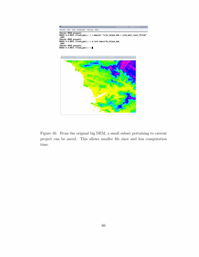
Figure 16: From the original big DEM, a small subset pertaining to current

project can be saved. This allows smaller file sizes and less computation

time.

66

Figure 17: Executing module r.watershed for the Talpona river region.

67

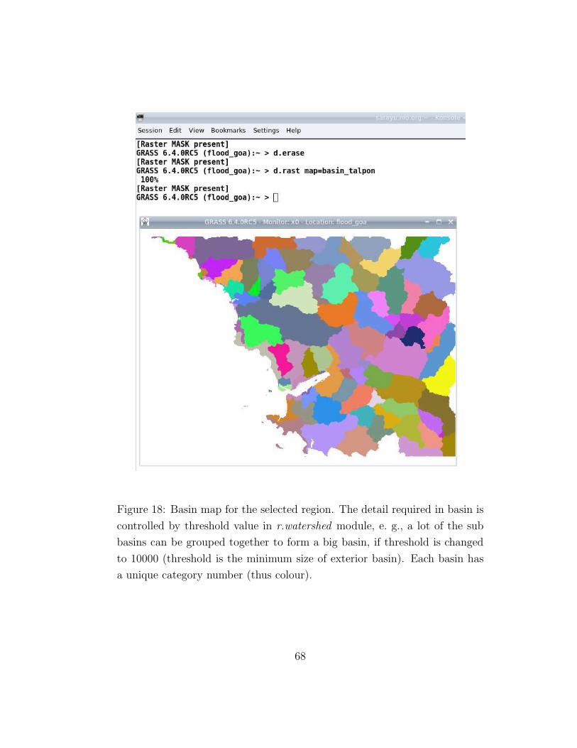
Figure 18: Basin map for the selected region. The detail required in basin is

controlled by threshold value in r.watershed module, e. g., a lot of the sub

basins can be grouped together to form a big basin, if threshold is changed

to 10000 (threshold is the minimum size of exterior basin). Each basin has

a unique category number (thus colour).

68

Figure 19: Stream network map for the selected region. Each stream has

a category number (shown by different colour), which is same as of corre-

sponding basin. To get a detailed stream network map, threshold need to be

lowered as only one stream per basin is shown.

69

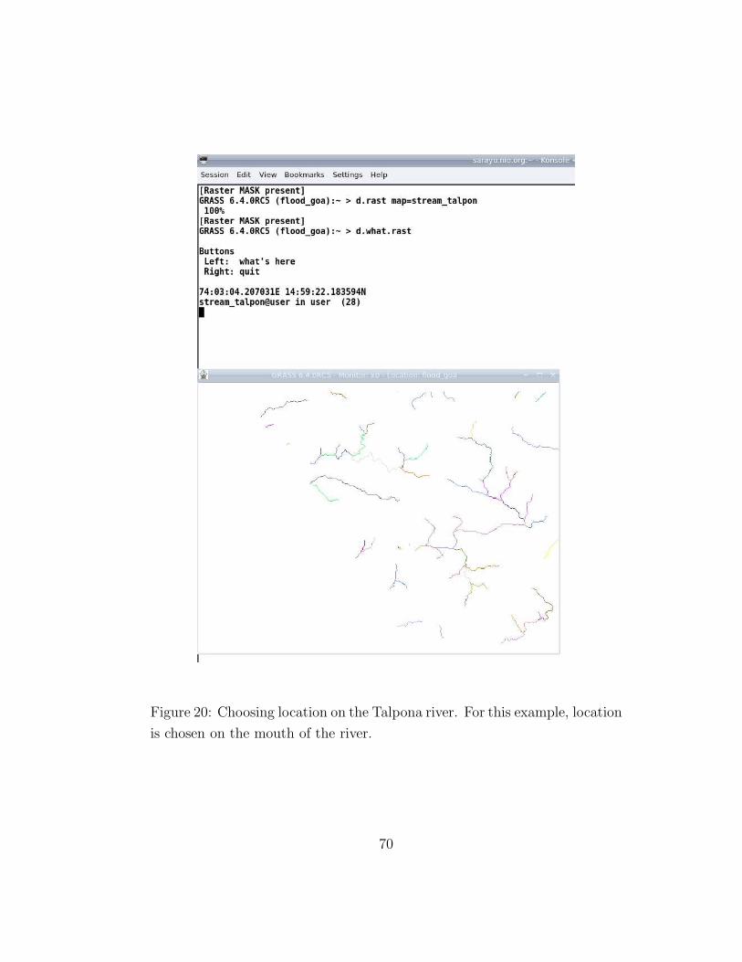
Figure 20: Choosing location on the Talpona river. For this example, location

is chosen on the mouth of the river.

70

Figure 21: Creating watershed area over the selected location. The area

plotted in red is the watershed area over the selected location.

Figure 22: Converting raster map of watershed to vector map.

71

Figure 23: Displaying vector watershed map. The thin black line marks the

watershed divide and “x” marked inside is centre (centroid) of the area.

72

Figure 24: Querying the vector map will give the area of the watershed. Area

is given in m2, hectares, square miles and acres.

73

Figure 25: Rational method calculation on a spreadsheet software. The area

is converted into km2 from the earlier output.

74