Marshall UniversityMarshall Digital Scholar

Theses, Dissertations and Capstones

1-1-2009

A GIS Analysis on Possible Photovoltaic Cell Usefor Energy Reduction During Peak Hours inHuntington, West VirginiaJames Eric Tadlock

Follow this and additional works at: http://mds.marshall.edu/etdPart of the Geographic Information Sciences Commons, Natural Resource Economics

Commons, Natural Resources and Conservation Commons, Physical and Environmental GeographyCommons, and the Sustainability Commons

This Thesis is brought to you for free and open access by Marshall Digital Scholar. It has been accepted for inclusion in Theses, Dissertations andCapstones by an authorized administrator of Marshall Digital Scholar. For more information, please contact zhangj@marshall.edu.

Recommended CitationTadlock, James Eric, "A GIS Analysis on Possible Photovoltaic Cell Use for Energy Reduction During Peak Hours in Huntington, WestVirginia" (2009). Theses, Dissertations and Capstones. Paper 331.

  

A GIS Analysis on Possible Photovoltaic Cell Use for Energy Reduction During Peak Hours

in Huntington, West Virginia

Thesis submitted to

The Graduate College of

Marshall University

In partial fulfillment of

The requirements for the degree of

Master of Science in Geography

by

James Eric Tadlock

Dr. Anita Walz, Ph.D., Committee Chairperson

Dr. Kevin Law, Ph.D.

Dr. Joshua Hagen, Ph.D.

Marshall University

May 2009

  

ABSTRACT

A GIS Analysis on Possible Photovoltaic Cell Use for Energy Reduction During Peak Hours

in Huntington, West Virginia

By James Eric Tadlock

Solar panels are one of the fastest growing renewable energy technologies. This study

aims to identify to what extent roof-mounted solar panels can reduce the need of power provided

by Appalachian Power Company. Data from the Reliability First Corporation was employed to

determine the individual average household power usage. Three study areas in Huntington,

West Virginia, were selected to determine if solar panels could be implemented. Roofs

in the study areas were digitized to calculate the available area. Based on the average

household usage, four different sized photovoltaic systems were determined. Potential power

production was computed to identify any offset of consumption from the power grid. The

average household roof size is sufficient to sustain a solar panel system that provides 75% or

more of the required energy.

iii  

ACKNOWLEDGMENTS

I would like to thank my thesis committee for their assistance in my pursuit of a graduate

degree, especially Dr. Anita Walz for serving as my advisor and committee chairperson. Her

guidance and mentoring has been greatly appreciated. I would like to mention thanks to

members of the Geography 530 – Raster Analysis class from the fall 2008 for their help in the

digitizing of the study areas and building footprints. Many thanks are devoted to Christine Risch

of the Center for Business and Economic Research at Marshall University. Her assistance

allowed for this research to be possible by allowing access to the Reliability First Corporation’s

regional power usage data obtained by her department. I would also like to recognize the

assistance provided by the Appalachian Power Company, Atlantic City Electric, and the

Reliability First Corporation. I thank them for the prompt responses they provided to the many

questions I asked them.

iv  

TABLE OF CONTENTS

Abstract ……………………………………………………………………………………………………ii

Acknowledgments ……………………………………………………………………………………….iii

List of Tables .…………….………………………………………………………………………………v

List of Figures ……………………………………………………………………………………………vi

Chapter One: Introduction ………………………………………………………………………………1

Solar Panel Research, Development, and Usage……………………………………………1

Current Power Production, Supply, and Usage in West Virginia…………………………...8

Chapter Two: Materials and Methods…………………………………………………………………14

Determination of Roof Areas in Huntington, West Virginia………………………………...14

Determination of Average Residential Power Consumption

in Huntington, West Virginia............................................................................................16

Estimation of Power Production by PV systems in Huntington, West Virginia…………..24

Chapter Three: Results ………………………………………………………………………………..28

Chapter Four: Conclusions and Discussion……………………………………………………….…37

Bibliography………………………………………………………………………………………...……41

v  

LIST OF TABLES

Table 1: West Virginia Power Usage Totals by Production Method……………………………….11

Table 2: Appalachian Power Company Power Plants ……………………………………………...11

Table 3: Power Plants within the Reliability First Corporation Boundaries ……………………….20

Table 4: Building Footprints Amount of Area Covered in Each Study Area ……………………...23

Table 5: Solar Panel System Specifications for Unit Studied ……………………………………...29

Table 6: Solar Panel System Area Compatibility with Huntington Buildings ……………………..29

Table 7: House PV System Compatibility…………………………………………………………….35

Table 8: Garage PV System Compatibility…………………………………………………………...36

Table 9: Maximum PV System for Commercial Buidlings…………………………………………..36

vi  

LIST OF FIGURES

Figure 1: Methods of Multicrystalline Cell Creation …...................................................................4

Figure 2: Cross-section of CIS Cells ………………………………………………………………..….6

Figure 3: Total Power Usage Peaks from the Reliability First Corporation ………………………..9

Figure 4: Maps of the Huntington Study Areas ……………………………………………………...15

Figure 5: NDVI Maps of the Ritter Park Study Area …................................................................17

Figure 6: NDVI Maps of the Hal Greer Study Area …………………………………………………18

Figure 7: NDVI Maps of the Downtown Study Area ………………………………………………...19

Figure 8: Reliability First Corporation Maps ………………………………………………………....22

Figure 9: Individual Household Power Usage Peaks ……………………………………………….25

Figure 10: Power Usage Offset Using a 2.1 kW System …………………………………………..31

Figure 11: Power Usage Offset Using a 4.2 kW System …………………………………………..32

Figure 12: Power Usage Offset Using a 6.3 kW System …………..………………………………33

Figure 13: Power Usage Offset Using a 8.4 kW System …………………………..………………34

1  

CHAPTER ONE: INTRODUCTION

With the increasing demand for energy and concern about carbon dioxide within the

United States, it is imperative that alternate energy sources be used to reduce the dependence

on fossil fuels. New innovations in “green” technology are needed to implement these changes.

One method of harnessing nature technologically is to produce energy through the use of

photovoltaic (PV) cells, more commonly called solar cells, which harness sunlight and convert it

into electric power. The objectives of this research are to a) compile information on the types of

solar panels and their availability to the Huntington, West Virginia area; b) report on current

solar panel usage incentives and or regulations made by governments and power industries in

the state; and c) to produce examples within areas of Huntington, West Virginia to show

feasibility or possible benefits from the installation of solar paneling on the roofs of housing or

commercial buildings through Geographic Information System (GIS) Analysis.

Solar Panel Research, Development, and Usage

There are two methods in the realm of collecting the sun’s energy to produce electricity.

The first of these methods is the use of parabolic shaped mirrors which concentrate the sun’s

thermal energy. The thermal energy is used to heat water into steam which then rotates

turbines that are connected to electric generators (Pitz-Paal, 2008). The second method is the

collection of the light from the sun in cells made from a semi-conductive material. Energy is

produced from the change of the energy state in electrons that occurs when photons from

sunlight interact with the semi-conductive material (Wengenmayr, 2008). This research will

focus on the latter of the two methods given that they are more compatible with home

installation. PV technology is steadily growing in popularity. Currently, PV system use is

increasing at a rate of approximately 25% per year (Komor, 2004). The most popular method of

use for PV systems is to connect to the already existing power grid to reduce the cost of electric

2  

bills. These grid-connected systems represent 50% to 70% of PV sales worldwide (Celik et al,

2008). As with many products, there are pros and cons related to its performance.

Some of the pros of PV systems are that they utilize the most plentiful source for energy,

they can be easily moved to and set up in more isolated areas (Komor, 2004), prices for PV

systems have decreased to a hundredth of their original costs and will continue to decline as

production increases (Aratani, 2005), and finally, PV systems are the most aesthetically

pleasing of the renewable sources if located in an urban setting. Some of the cons for solar

panel systems include that they are still expensive even with decreases in cost, PV systems do

not produce energy during the night (Komor, 2004), and lastly, maintenance costs for

replacement of damaged PV modules, storage batteries (if used), electrical systems, and other

vital devices can be expensive (Canada et al, 2005).

The first working PV system was created in 1883 by an American by the name of

Charles Fritts. Fritts’ selenium cell had an efficiency of >1%, which is considered low by today’s

standards. The first modern PV systems were produced by Chapin, Fuller, and Pearson in

1953 and 1954 under Bell Labs in the United States. Efficiencies produced are limited by the

material used and by the fragile balance of cost and intricacy of the cell (Twidell and Weir,

2006). Early silicon cells reached efficiencies between 4.5% and 6%. With continuing research,

today’s systems are reaching efficiencies of up to 39% (Wengenmayr, 2008). According to

Twidell and Weir ( 2006), more common commercial systems of today stay within the range of

10% to 22% in normal lighting conditions.

Two forms of PV cells are now being produced and researched, crystalline silicon and

thin film. There are currently three kinds of silicon systems: monocrystalline, multicrystalline

and amorphous silicon. Together, silicon systems account for approximately 92% of the world’s

PV usage (Aratani, 2005). Monocrystalline PVs are the most expensive units to produce due to

3  

the high cost of pure silicon that is used to create the cells. The cells are sliced from blocks of

refined silicon called ingots. Ingots are cooled at controlled rates to create the single crystalline

form. After cooling is complete, the ingots are sliced to a thickness between 200 and 300 µm.

This process wastes over 50% of the pure silicon in the cutting procedure (Hahn, 2008). After

cell completion, monocrystalline cells have commercial efficiencies around 15% and laboratory

efficiencies at or near 25% (Twidell and Weir, 2006).

Multicrystalline cell production methods were developed to reduce the amount of waste

through the production process. This allows more cells to be created; therefore, reducing the

cost of the cell itself. In multicrystalline (also called ribbon silicon) production, rather than all of

the molten silicon being cooled at a controlled rate, the cell is formed in one of three ways. The

first method, which is called Edge-defined Film-fed Growth (EFG), pulls the silicon through a

mould via capillary action while attached to a solid (Figure 1a). The silicon is continually pulled

vertically at a rate of 1 to 2 cm/min as it cools while it is formed into octagonal columns. The

eight sides are cut separately and then cut into smaller, more familiar PV cells (Hahn, 2008).

Not too dissimilar from the EFG method, the second method uses two “strings”, made of

a material which manufacturers keep undisclosed, instead of moulds (Figure 1b). The silicon is

pulled into sheets vertically, laid out, and then cut with lasers to specified dimensions.

Manufacturers are able to pull the silicon into sheets due to its high tension strength. The

thickness of these sheets is thinner than its mould formed counterpart due to the stretching

between the two strings. This method produces the sheets at similar rates of 1 to 2 cm/min like

that of the EFG method (Hahn, 2008).

The final method in multicrystalline cell fabrication is called Ribbon Growth on Substrate

(RGS). Instead of the silicon being lifted vertically, it is spread horizontally across a substrate

(Figure 1c). A belt rolls the substrate under a crucible containing melted silicon. While being

Mol

ten

Si

Molten Si

Molten Si

Mou

ld

Mou

ld

Solid

Solid

Dire

ctio

n of

Mov

emen

t

Dire

ctio

n of

Mov

emen

t

Direction of

Movement

a b

c

Figure 1. Simplified drawings of the three multicrystalline silicon cell creation methods as adapted from Hahn, 2008. a) The EFG method. b) V ertical pulling method using strings (strings are not illustrated). c) RGS method.

5  

rolled, the melted silicon is poured onto the substrate. As the silicon cools, it separates from the

substrate due to differences in the expansion coefficients of the two materials. This method is

the fastest of the three production methods for multicrystalline PV cells with rates of 10 cm/s.

Unfortunately, this method is not in commercial use due to its being in experimental stages

(Hahn, 2008). Twidell and Weir (2006) state that the three types of multicrystalline cells

lproduce 8% to 13% efficiencies for commercial users and roughly 16% to 20% efficiencies for

laboratory use.

Amorphous silicon cells are created similarly to thin-film cells in that they are both placed

on a substrate in very thin layers. Instead of using numerous types of chemical elements like

the thin-films, very thin layers of silicon that have had hydrogen added during the preparation

procedures are utilized. The use of hydrogen allows for the repair of some defects, such as

misalignments in the crystal lattice, that might have formed in normal silicon cooling.

Unfortunately, amorphous silicon is the least stable in efficiencies. After the first uses, the

efficiencies can drop by as much as 30% from the original efficiency of 15% (Guha and Yang,

2005; Wegenmeyr, 2008). Therefore, even though it is used in building integrated PV systems,

it is not commonly employed in commercial PV systems (U.S. Department of Energy, 2009;

Wengenmeyr, 2008).

Thin film PV systems were first explored in 1999 by the Hahn-Meitner Institute of

Germany. After several years of research, the first thin film units were placed on the market in

2006. Thin film systems are created by the layering of multiple materials on a substrate such as

glass (Figure 2). The most common material used for thin film units is a copper, indium, and

sulfur (CuInS2) mixture, otherwise known as CIS. This material is able to completely absorb

sunlight in layers as thin as 1 μm. More commonly, it is applied to the substrate in a layer of

about 1.5 μm. This allows for approximately one hundredth of the material to be used and more

to be manufactured as compared to monocrystalline silicon units. With other materials placed

Substrate

Backing Electrode

CIS Material

1.1μm

1.5μm

0.5μm

~2mm

Front Electrode and Lamination Material

Figure 2. A cross sesction of a CIS PV cell as adapted from Meyer, 2008.

7 

beneath and above the CIS material to complete the circuit, total thickness is near 3 μm (Meyer,

2008).

The benefits of this type of PV cell compared to silicon systems is that thin-film units

require two-thirds less energy to assemble and one-third the number of steps. These benefits

allow for the overall cost of the unit to be reduced (Meyer, 2008). With thinner systems, more

items and buildings can be built with PV systems already incorporated in the building materials.

One example of which is roofing materials (Komor, 2004). Efficiencies for thin-film systems

range between 8% at lowest, 13% to 15% at its highest, and proposed efficiencies of 25%

(Meyer, 2008; Twidell and Weir, 2006).

Performance and maintenance are issues with which all PV system owners must

contend. Before any system is made available to the market, the International Organization for

Standardization (ISO) tests each model of PV system with a Life Cycle Assessment that is

made of four parts. The first of these parts is the goal and scope which is used to identify the

limits of each PV system. Inventory analysis is used to research what materials were utilized for

the unit. The impact assessment is evaluated to identify any emissions and byproducts that are

created in the production process and if they pose any harm to the environment. The final step,

interpretation, includes the conclusions associated with the performance of the PV system

(Jungbluth, 2004).

Although these steps are implemented, owners of PV systems can still see a 50%

malfunction rate mostly due to improper installation. These include, but are not limited to, lack

of safety equipment and inadequacies in durability and performance materials. These

operational costs can equate to between 5% and 6% of overall cost for the PV system (Canada

et al, 2005). It is necessary, however, to maintain the PV system in order to generate sufficient

8  

electricity over the years. The main factors that can keep a PV system operational are element

quality and the availability of repair services and replacement parts (Díaz et al, 2007).

Research conducted by Dunlop and Halton (2006) suggests that silicon PV systems with

proper maintenance can last over 20 years. The systems studied were constructed between

the years of 1982 and 1984. Dunlop and Halton compared the functionality of the systems in

2004 to the original functionality from the manufacturer’s data. The data from Dunlop and

Halton (2006) showed that 80% of the cells tested only lost approximately 9.5% or less of their

original electricity production efficiency after 20 years. The 20-year old cells were still capable

of producing enough electricity to sustain the user’s demands but were not recommended for

use beyond 25 years because of the degradational effects of weathering on the cell material.

After a PV system has reached the end of its service life, the silicon in the PV cells and the

metals for the PV body and brackets can be recycled to decrease the amount of waste

(Jungbluth, 2005).

Current Power Production, Supply, and Usage in West Virginia

Power data are collected by the power companies and forwarded to organizations that

monitor the fluctuations of usage in regions across the United States. The Reliability First

Corporation (RFC), which surpervises the Appalachian Power Company, is one such

organization. The RFC creates and imposes regulations for the use and distribution of bulk

power systems for its region (Whitely and Gallagher, 2008).

Hourly data per day for every month was used to show peaks that occur during the

various hours of the day (Figure 3). In the RFC region, higher peaks occur during the late

morning hours, decline slightly in the afternoon, and peak again in the evening. Higher power

usage can be seen in the winter and summer months due to combative measures against

70

80

90

10

0

11

0

12

0

13

0

14

0

15

0

12

34

56

78

91

01

11

21

31

41

51

61

71

81

92

02

12

22

32

4

Power Usage (Thousands of MWh)

Hou

rs o

f th

e da

y

Jan

uar

y

Feb

ruar

y

Mar

ch

Ap

ril

May

Jun

e

July

Au

gust

Sep

tem

ber

Oct

ob

er

No

vem

ber

Dec

emb

er

Figu

re 3

. R

FC re

gion

hou

rly p

ower

use

per

ave

rage

day

in a

mon

th fr

om 2

008.

Eac

h se

ason

ha

s be

en g

iven

a c

olor

sch

eme:

blu

e fo

r win

ter, g

reen

for s

prin

g, re

d fo

r sum

mer

, and

ora

nge

for

fall.

Th

is c

olor

sch

eme

will

rem

ain

cons

ista

nt th

rouh

out t

he s

tudy

. Th

e ve

rtica

l das

hed

lines

re

pres

ent t

imes

whe

n pe

aks

in p

ower

con

sum

ptio

n be

gin

and

end.

10  

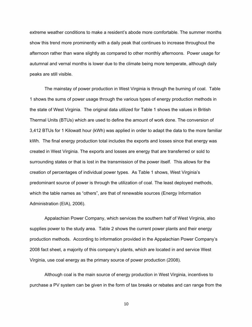
extreme weather conditions to make a resident’s abode more comfortable. The summer months

show this trend more prominently with a daily peak that continues to increase throughout the

afternoon rather than wane slightly as compared to other monthly afternoons. Power usage for

autumnal and vernal months is lower due to the climate being more temperate, although daily

peaks are still visible.

The mainstay of power production in West Virginia is through the burning of coal. Table

1 shows the sums of power usage through the various types of energy production methods in

the state of West Virginia. The original data utilized for Table 1 shows the values in British

Thermal Units (BTUs) which are used to define the amount of work done. The conversion of

3,412 BTUs for 1 Kilowatt hour (kWh) was applied in order to adapt the data to the more familiar

kWh. The final energy production total includes the exports and losses since that energy was

created in West Virginia. The exports and losses are energy that are transferred or sold to

surrounding states or that is lost in the transmission of the power itself. This allows for the

creation of percentages of individual power types. As Table 1 shows, West Virginia’s

predominant source of power is through the utilization of coal. The least deployed methods,

which the table names as “others”, are that of renewable sources (Energy Information

Administration (EIA), 2006).

Appalachian Power Company, which services the southern half of West Virginia, also

supplies power to the study area. Table 2 shows the current power plants and their energy

production methods. According to information provided in the Appalachian Power Company’s

2008 fact sheet, a majority of this company’s plants, which are located in and service West

Virginia, use coal energy as the primary source of power production (2008).

Although coal is the main source of energy production in West Virginia, incentives to

purchase a PV system can be given in the form of tax breaks or rebates and can range from the

Fuel Type BTUs kWH %Coal 9.59E+14 2.81E+11 48.64

NaturalGas 1.28E+14 3.75E+10 6.49

Petroleum 2.92E+14 8.55E+10 14.79

Hydro-Electric 1.56E+13 4.57E+09 0.79

Biomass 4.40E+12 1.29E+09 0.22

Other 1.80E+12 5.28E+08 0.09

Exports/Losses 5.71E+14 1.67E+11 28.97

Total 1.97E+15 5.78E+11 n/a

Power Production Methods of West Virginia

Table 1. Totals of power production from varying types of energy sources for the state of W est V irginia as adapted from the Energy Information Administration (2006).

Plant Name Plant Type Capacity (MW)John E. Amos Coal 2900

Mountaineer Coal 1320

Phillip Sporn Coal 1050

Kanawha River Coal 400

Total 5670Ceredo Natural Gas 505

Winfield Hydro 14.7

London Hydro 14.4

Marmet Hydro 14.4

Total 43.5

Energy Generation Types by Appalachian Power Co.

Table 2. Power plant names, types, and capacities for each plant and power gen-eration type that is operated by Appalachian Power Company in W est V irginia (adapted from Appalachian Power Fact Sheet, 2008).

12  

city level to federal relief. In the United States, a federal tax credit of 30% of the system cost is

given to a PV system owner when filing income taxes. Some states offer buyers as much as

$24,000 in rebates to help reduce the initial cost of a PV system (BP Solar, 2009). The top

three states that offer the largest incentives are Louisiana, Oregon, and Connecticut

respectively. These states are rated high because of their substantial state tax rebates for

purchasing a PV system. Louisiana offers a 50% price reduction on the first $25,000 of the

system cost and the federal tax incentive of 30%. Oregon and Connecticut offer similar tax

breaks including utility tax breaks of varying amounts from the local utility companies

themselves and exemption of sales tax on the systems purchased. West Virginia is ranked last

with Tennessee for solar power incentives. No state incentives are offered by either state (Find

Solar, 2009). Most of the incentives in West Virginia that are given to buyers of any “green”

energy are those who have utilized wind based technologies (West Virginia State Legislature,

2001).

Unfortunately, some power companies limit the amount of power that can be produced

from solar cells. Appalachian Power Company allows a homeowner’s PV system to be

connected to the company’s grid as long as the system does not exceed a producing capacity of

more than 25 kW. The system may be used for partial to complete reduction of the amount of

energy purchased from the company. Any power generated in excess of the household’s needs

can only be credited to the homeowner for a period of 12 months. Anytime after that period,

Appalachian Power claims what has been generated without reimbursement to the producer

(Appalachian Power Company, 2007).

As an alternative to purchasing a PV system, some companies have been formed that

allow homeowners to rent PV systems. The agreement starts with a down-payment that is

returned at the end of the contract. The household remains connected to the energy grid, and

13  

monthly payments are made to both the power company and the PV rental company. The

payments would be the same or less as if a household were solely dependent on the power

company or if a private PV system was owned (Citizenrē Corporation, 2009). The household is

liable to be in accordance of the net-metering laws that the utility company has issued and are

bound to arrange for any changes that may occur in these laws (Citizenrē Corporation, 2007).

The monthly rate owed to the PV rental company is kept constant from the time of signing of the

contract. Whenever repairs need to be made, the company will repair the system free of

charge. This allows for the use of “green” systems without the aggravations of complete system

upkeep (Citizenrē Corporation, 2009).

Assisted by the information researched above, a study for power usage and its reduction

via solar panels systems was conducted for several Huntington, West Virginia neighborhoods.

Data compiled, including information from the Huntington area, shows how the location could

benefit from this renewable energy source.

14  

CHAPTER TWO: MATERIALS AND METHODS

Determination of Roof Areas in Huntington, West Virginia

The maps created in this section were generated using ArcMap 9.3 from ArcInfo™ by

Environmental System Research Institute (ESRI). One aerial photograph and one satellite

image were employed to complete this task. The SAMB Image, an aerial photograph, contains

high resolution cells of 60 cm. The SAMB is a true color image that contains the blue, green,

and red color bands. The satellite based IKONOS image was incorporated into this research for

two main reasons. It is a multispectral image that contains the near infra-red (NIR) band along

with the previous mentioned bands, and the image was taken during a time of the year when

vegetation was fully present. The latter fact is beneficial since it gives a good representation of

how much sun a roof could receive after being shaded by trees. The resolution is coarser in this

image with a cell size of 4 meters.

Three study areas were created and are referred to as the Ritter Park (RP) study area,

the Hal Greer Boulevard (HG) study area, and the Downtown (DT) study area (Figure 4). The

Downtown study area was chosen to represent the commercial zone of Huntington, West

Virginia. The Hal Greer and Ritter Park study areas represent typical residential and wealthy

residential zones respectively. Each study area consisted of four individual blocks which were

selected randomly. Polygons for the blocks and the buildings in each block were digitized into

vector files. Using the calculate geometry tool in ArcMap, the area for each building footprint

polygon was measured.

A Normalized Difference Vegetation Index (NDVI) is most commonly used to observe

changes in the amount of vegetation globally, but it can be used in a more localized setting

(Trishchenko et al, 2002). The NDVI calculation was used to determine the sealed and

vegetated areas within the City of Huntington (Equation 1). The NDVI is calculated as follows:

Stud

yA

reas

ofH

untin

gton

,W.V

.R

itter

Park

Stud

yAr

eas

Hal

Gre

erSt

udy

Area

sD

ownt

own

Stu

dyAr

eas

§0

0.5

10.

25Ki

lom

eter

s

1:15

,000

RP1

RP3

RP2

RP4

HG

4

HG

3

HG

1

HG

2

DT1

DT4

DT3

DT2

Figu

re 4

. a)

SA

MB

imag

e w

ith R

itter

Par

k (R

P) s

tudy

are

as h

igh-

light

ed in

blu

e. b

) S

AM

B im

age

with

Hal

Gre

er (H

G) s

tudy

are

as

high

light

ed in

yel

low.

c)

SA

MB

imag

e w

ith D

ownt

own

(DT)

stu

dy

area

s hi

ghlig

hted

in re

d. N

umbe

rs la

belin

g th

e st

udy

area

s w

ill

rem

ain

cons

ista

nt in

sub

sequ

ent f

igur

es.

a c

b

16  

Equation 1

The ρNIR represents the wavelength of the NIR band and ρRed denotes the wavelength of

the Red band of the IKONOS image. The NDVI shows the presence and variations of green

biomaterials (Jensen, 2005). Cell values range between -1 and 1. The lower values represent

mostly sealed or non-vegetated surfaces and water, while the higher values signify presence of

vegetation. A cut off value of 0.3 was used to distinguish between the difference of vegetated

and non-vegetated surfaces. This cut off value was determined through the comparison of the

location of the vegetation in the NDVI result and the original IKONOS and SAMB images. The

raster calculator in ArcMap was used to calculate the NDVI. The image was then classified into

1 (NDVI ≥ 0.3; vegetation) and 0 (NDVI ≤ 0.3; sealed surfaces) with the use of a conditional

statement.

The NDVI was then clipped to the four blocks of each of the three study areas using the

polygons of the blocks that were created earlier. The two colors of the newly clipped NDVIs

were darkened to highlight the study areas against the city-wide NDVI. The polygons of the

building footprints were included in order to show which sealed surfaces were due to roofing

and to show if there was any significant vegetation overlapping the roof’s surface that might

prevent sunlight from reaching the possible locations of a PV system (Figures 5, 6, and 7 for

RP, HG, and DT respectively). Table 3 shows the results of the GIS analysis, which include the

amount of surface area that is covered by roofs, concrete or asphalt, total sealed surfaces (roofs

and other sealed surfaces), and total area of sealed and vegetated surfaces.

Determination of Average Residential Power Consumption in Huntington, West Virginia

To determine what system is most suitable for a commercial or residential building in the

Huntington area, data from power usage, solar irradiance, and photovoltaic system

specifications were obtained. Information about the distribution and amounts of power usage

015

030

075

Met

ers

§

Stud

yA

rea

Surf

ace

Type

s

Seal

ed

Vege

tatio

n

Build

ing

City

Surf

ace

Type

s

Seal

edVe

geta

tion

Figu

re 5

. C

lass

ified

ND

VI i

mag

e to

sho

w th

e ar

eas

cove

red

by

seal

ed s

urfa

ces

or v

eget

atio

n fo

r the

Ritt

er P

ark

stud

y ar

eas.

Bui

ldin

g fo

otpr

ints

are

giv

en to

sho

w w

hich

sea

led

surfa

ces

are

roof

s. a

) RP

1 in

the

low

er le

ft an

d R

P2

in th

e up

per r

ight

. b)

RP

3. c

) RP

4.

a c

b

015

030

075

Met

ers

§

Stud

yA

rea

Surf

ace

Type

s

Seal

ed

Vege

tatio

n

Build

ing

City

Surf

ace

Type

s

Seal

edVe

geta

tion

Figu

re 6

. C

lass

ified

ND

VI i

mag

e to

sho

w th

e ar

eas

cove

red

by

seal

ed s

urfa

ces

or v

eget

atio

n fo

r the

Hal

Gre

er s

tudy

are

as.

B

uild

ing

foot

prin

ts a

re g

iven

to s

how

whi

ch s

eale

d su

rface

s ar

e ro

ofs.

a) H

G1.

b)

HG

2. c

) H

G3

in th

e up

per l

eft a

nd H

G4

in th

e lo

wer

righ

t.

a c

b

015

030

075

Met

ers

§

Stud

yA

rea

Surf

ace

Type

s

Seal

ed

Vege

tatio

n

Build

ing

City

Surf

ace

Type

s

Seal

edVe

geta

tion

Figu

re 7

. C

lass

ified

ND

VI i

mag

e to

sho

w th

e ar

eas

cove

red

by

seal

ed s

urfa

ces

or v

eget

atio

n fo

r the

Dow

ntow

n st

udy

area

s.

B

uild

ing

foot

prin

ts a

re g

iven

to s

how

whi

ch s

eale

d su

rface

s ar

e ro

ofs.

a) D

T1 in

the

uppe

r lef

t and

DT2

in th

e lo

wer

righ

t. b

) D

T3.

c) D

T4.

a c

b

Table 3. Raster analysis showing the area covered by roof surfaces, other sealed surfaces, and total sealed surfaces (other sealed and roof) for the Ritter Park (RP), Hal Greer (HG), and Downtown (DT) study areas. Roof values are before division by two to calculate available roof area for PV systems.

Study AreaRoof Area

(sq-m)

Other Sealed

Area

(sq-m)

Total Area

(sq-m)

%

Roof

%

Other

Sealed

%

Total

Sealed

RP1 3297.11 2480.84 17846.02 18.48 13.90 32.38

RP2 4177.41 5089.72 22887.72 18.25 22.24 40.49

RP3 3953.33 4081.38 23063.78 17.14 17.70 34.84

RP4 4273.44 5249.77 23527.94 18.16 22.31 40.48

HG1 7842.65 10131.42 32074.82 24.45 31.59 56.04

HG2 2288.77 2768.93 10627.59 21.54 26.05 47.59

HG3 5473.85 5585.88 23223.84 23.57 24.05 47.62

HG4 2704.91 2112.71 11603.92 23.31 18.21 41.52

DT1 16693.63 10195.44 28617.66 58.33 35.63 93.96

DT2 4785.61 10419.52 21015.09 22.77 49.58 72.35

DT3 6546.21 15493.23 24344.21 26.89 63.64 90.53

DT4 7122.40 15093.09 22759.68 31.29 66.32 97.61

GIS Analysis Results

21  

were not readily available. If data exist at all, some were not accessible to public use. Some

power companies were not willing to release data about the number of customers they served,

the distribution of electrical power throughout their service locations, or how much an average

commercial customer used in comparison to an average residential customer. Some data could

only be retrieved if membership to the corporation was obtained. These memberships could

range from $200 to over $1,000. Other forms of data could be purchased, but at prices as steep

as $5,000. Prices of that magnitude were beyond the scope of this study.

Three assumptions were made in order to conduct this research. No data corresponding

to the number of commercial consumers could be found for the RFC region. Not all power

companies release specific values of the number of customers using their services, so an exact

number of households could not be determined. Consequently, the first assumption was that

the number of households matches general patterns of the RFC boundaries via the county

boundaries within its participating localities (Figure 8); therefore, the census data for those

counties yield a good estimate of the number of households serviced by the company. In

reality, all households use energy at different rates; however, for the purpose of this study, all

residences are assumed to use energy at the same rate. The final assumption made is that

each household has its own roof. Power usage data for commercial buildings was not available;

therefore, the size of the PV system required could not be estimated. Instead, the roof areas of

the downtown study area were used to approximate the maximum capacity of the PV system

they would be able to support.

The data from the RFC originally was total power usage for every hour of the year of

2008 across the RFC region in Megawatt-hours (MWh). Based on information from the EIA

(2009), a total of 96 power plants (Table 4) supply the RFC region with electricity totaling

936,209,202 MWh (RFC, 2009). Within this region there are a total of roughly 26,946,000

State Boundaries

RFC Region

§0 250 500125

Kilometers

Figure 8. a) A map of the Reliability Corporations of North America including the RFC (North American Electric Reliability Corporation, 2009). b) Map created using ArcMap and TIGER/Line county census 2000 data to gain information about the area covered and the number of households in the RFC region.

States

a

b

State Nuclear Petroleum CoalNatural

GasGeo-

thermalSolar

Hydro-electric

Wind

VA 0 1 2 1 0 0 0 0

MD 1 7 8 8 0 0 1 0

DE 0 2 2 3 0 0 0 0

NJ 3 6 5 21 0 0 1 0

PA 5 6 24 15 0 0 4 0

WV 0 0 14 3 0 0 0 0

OH 2 3 21 15 0 0 0 0

IN 0 1 21 18 0 0 0 0

KY 0 0 11 2 0 0 2 0

IL 5 2 7 17 0 0 0 0

MI 3 1 13 21 0 0 1 0

WI 0 1 6 12 0 0 0 0

Powerplants of the RFC Region

Table 4. The numbers and types of power plants present within the RFC region (EIA, 2009).

24  

households with an average household size of 2.52 people dispersed across approximately

663,140 km2. The total number of households and average household size were obtained from

county-wide 2000 census data collected by the United States Census Bureau and were based

on the shape of the service area of the RFC.

The total power load for each hour was multiplied by 1000 to convert it into kWh. As

indicated by the Annual Energy Review by the EIA (2007), 30% of the energy generated by

power plants is consumed by residential customers; therefore, the total power load was

multiplied by 0.3 to produce the amount of energy that is used by the residents of the RFC.

Lastly, the power used by RFC residents was divided by the total number of households from

the RFC region to show the average power usage per hour for an average individual residence.

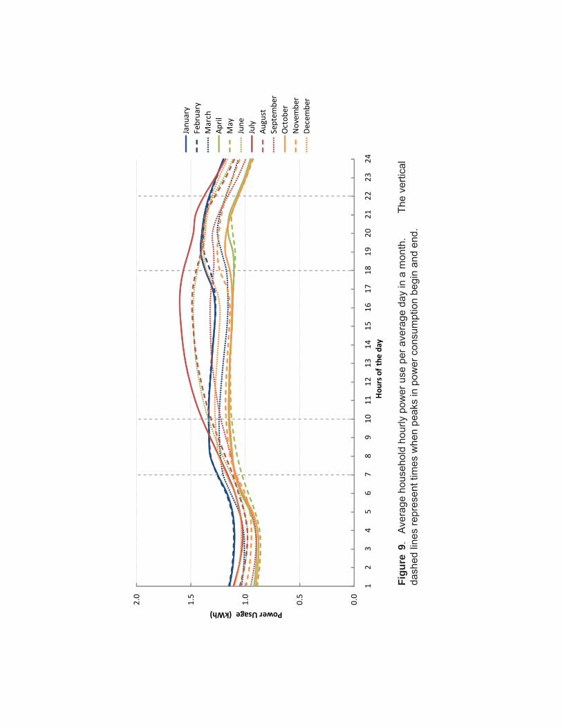
Figure 9 shows the peaks of power usage by a typical household on an average day in each

month. The peaks show a similarity to that of the regional usage, but at a smaller scale. During

the winter, spring, and fall months, peaks occurred between the 7th and 10th hours of the day

and the 18th and 22nd hours. In the summer months and one spring month, a peak forms around

the 7th hour but continues to increase throughout the day instead of leveling off during the mid-

morning and do not decrease until about the 22nd hour of the day.

Estimation of Power Production by PV Systems in Huntington, West Virginia

To see the effects that a grid- connected solar panel system would have on an average

household in Huntington, an equation to determine the output of a solar panel based on solar

irradiance was used.

⁄ Equation 2

The EPV represents the power production by a PV unit at a given time in kWh. PPV is the

maximum amount of power the PV system can produce in kW. The symbol denotes the

efficiency of wiring and components used in the system which has a constant of 0.9 for all

0.0

0.5

1.0

1.5

2.0

12

34

56

78

91

01

11

21

31

41

51

61

71

81

92

02

12

22

32

4

Power Usage (kWh)

Hou

rs o

f th

e da

y

Jan

uar

y

Feb

ruar

y

Mar

ch

Ap

ril

May

Jun

e

July

Au

gust

Sep

tem

ber

Oct

ob

er

No

vem

ber

Dec

emb

er

Figu

re 9

. Av

erag

e ho

useh

old

hour

ly p

ower

use

per

ave

rage

day

in a

mon

th.

The

verti

cal

dash

ed li

nes

repr

esen

t tim

es w

hen

peak

s in

pow

er c

onsu

mpt

ion

begi

n an

d en

d.

26  

systems. KPV signifies the reduction coefficient for the working conditions of a PV system and

has a constant of 0.8. The final ratio of S/ISTC is a comparison of the actual average solar

irradiance for every month in kWh/m2 at Huntington, West Virginia (S) divided by the solar

irradiance that was generated in standard testing conditions (ISTC) which is maintained

continually at 1 kW/m2. The West Virginia solar irradiance data (S) was gained from the

Cooperative Networks For Renewable Resource Management (CNFRRM) from a data

collection site at Bluefield State College in Bluefield, West Virginia. Data from this collection site

was measured from 1997 to 2008. Hourly data for every day from 1997 to 2004 was compiled

since it was the most complete data of the years given. These values were calculated into

average solar irradiation for an hour per month to correspond with the average hour per month

power usage values calculated from the RFC. This was done to construct typical weather

conditions for the Huntington area. Since the irradiation data was originally in Watt-hours/m2

(Wh/m2), it was diveded by 1000 to convert it into kWh/m2 which is more compatible with the

average residential power usage data.

The system sizes first mentioned were selected using the Solar Calculator, a tool

created by the Seattle-based company, Cooler Planet. The calculator requires a zip code, the

power utility company used, the average monthly electric bill or an average monthly power

usage in kWh, whether the location is residential or commercial, and how much energy offset is

desired in percent reduction (Cooler Planet, 2009). For this study, the zip code 25701 was used

and the residential button was selected. Appalachian Power was chosen from a drop-down list

of utility companies. The average monthly power consumption value of 883.1 kWh, which was

calculated earlier from the hourly usage data from the RFC, was utilized for the average monthly

power usage. Results of system specifications, which include kW production capacity, area

covered, and estimated costs before and after incentives and tax breaks, are returned

instantaneously.

27  

Four different power level systems were used for the PPV, which include: 2.1 kW, 4.2 kW,

6.3 kW, 8.4 kW systems. The four mentioned systems represent a 25%, 50%, 75%, and 100%

power reduction respectively on an average customer’s power usage in the RFC region. The

8.4 kW system hypothetically could fulfill any demands from an average household although,

Appalachian Power allows a homeowner to incorporate a system as large as 25 kW

(Appalachian Power Company, 2007).

To demonstrate the effect that a solar panel system would have on a household’s power

usage the following equation was used:

Equation 3

PAdj represents the adjusted power usage after a PV system has been implemented. P0

signifies the power usage before the PV system has been installed. The EPV, which was

calculated above, stands for the possible power produced by a solar panel. This step was used

for every hour of an average day for every month.

28  

CHAPTER THREE: RESULTS

Table 5 shows the number of buildings and their sizes corresponding to each of the

study locations and the areas covered by the building footprints. The building footprint is a

proxy for the amount of area that can be used to place a PV system. The residential footprint

area is cut in half due to the angled nature of a majority of housing roofs that face the proper

direction for collection of solar rays. The largest area covered by a building is the Big Sandy

Superstore Arena (DT1). The smallest area covered is by houses in the Hal Greer study area

(HG3). The average building footprint calculated for all commercial buildings is 6414.27 m2,

while the average building area available for solar panel installation for all residential structures

is 81.54 m2 without garages. Garages have an average area of 29.12 m2 available for PV

system installation.

The area covered by the IKONOS image is roughly 48.9 km2. The NDVI shows that

within this area approximately 68.6% of the surfaces are classified as vegetation, while the

sealed surfaces account for nearly 15.4 km2, or 31.40%. The DT1 study area has the largest

percentage of area covered by roof with 58.33%, while the smallest area covered by roofing

was in the RP3 study area with 17.14% (Table 3).

Table 6 gives the details of the various solar panels suggested by Cooler Planet. The

price range before the 30% tax reduction, the maximum incentive in West Virginia, would be

from $16,690.48 for a system that would be able to reduce power usage from the power

company by 25%, to $66,761.91 for a PV system that could supply nearly complete

independence from the power grid. Calculating the use of the federal tax incentive in West

Virginia, the price range of the systems would be from $11,683.34 to 46,733.34. If the

incentives from Louisiana were applied to these prices, they would range from $3,338.10 to

$34,233.34. The average monthly usage of power per hour in a day would decrease from

1.1867 kWh to 0.9656 kWh with a 2.1 kW system and 0.3025 kWh with a 8.4 kW system.

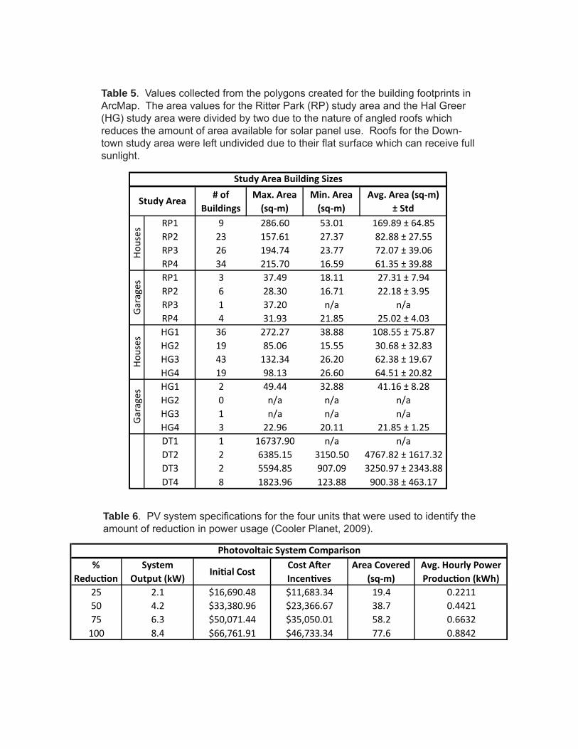
Table 5. Values collected from the polygons created for the building footprints in ArcMap. The area values for the Ritter Park (RP) study area and the Hal Greer (HG) study area were divided by two due to the nature of angled roofs which reduces the amount of area available for solar panel use. Roofs for the Down-town study area were left undivided due to their flat surface which can receive full sunlight.

# ofBuildings

Max. Area(sq-m)

Min. Area(sq-m)

Avg. Area (sq-m)± Std

RP1 9 286.60 53.01 169.89 ± 64.85

RP2 23 157.61 27.37 82.88 ± 27.55

RP3 26 194.74 23.77 72.07 ± 39.06

RP4 34 215.70 16.59 61.35 ± 39.88

RP1 3 37.49 18.11 27.31 ± 7.94

RP2 6 28.30 16.71 22.18 ± 3.95

RP3 1 37.20 n/a n/a

RP4 4 31.93 21.85 25.02 ± 4.03

HG1 36 272.27 38.88 108.55 ± 75.87

HG2 19 85.06 15.55 30.68 ± 32.83

HG3 43 132.34 26.20 62.38 ± 19.67

HG4 19 98.13 26.60 64.51 ± 20.82

HG1 2 49.44 32.88 41.16 ± 8.28

HG2 0 n/a n/a n/a

HG3 1 n/a n/a n/a

HG4 3 22.96 20.11 21.85 ± 1.25

DT1 1 16737.90 n/a n/a

DT2 2 6385.15 3150.50 4767.82 ± 1617.32

DT3 2 5594.85 907.09 3250.97 ± 2343.88

DT4 8 1823.96 123.88 900.38 ± 463.17

Gar

ages

Study Area

Study Area Building Sizes

Ho

use

sG

arag

esH

ou

ses

Table 6. PV system specifications for the four units that were used to identify the amount of reduction in power usage (Cooler Planet, 2009).

%Reduction

System Output (kW)

Initial CostCost AfterIncentives

Area Covered(sq-m)

Avg. Hourly PowerProduction (kWh)

25 2.1 $16,690.48 $11,683.34 19.4 0.2211

50 4.2 $33,380.96 $23,366.67 38.7 0.4421

75 6.3 $50,071.44 $35,050.01 58.2 0.6632

100 8.4 $66,761.91 $46,733.34 77.6 0.8842

Photovoltaic System Comparison

30  

Figures 10, 11, 12, and 13 show the effects of PV system implementation. With a

minimum system of 2.1 kW, a residence can reduce their power usage by approximately 0.2211

kWh per hour during times of sunlight. With the larger 8.4 kW system, power can be reduced

on average by 0.8842 kWh per hour during the day time hours.

Table 7 depicts four potential PV systems that may be suitable for a residence by

comparing the area the PV system occupies against the area available on the roof. Table 8

illustrates the possible use of garages from the study areas to employ more PV systems if a

homeowner wished to produce more energy, either to increase the percentage of independence

from the power company or to exceed the 100% independence and store it with batteries should

the option be available. The buildings of the downtown study areas far surpassed the available

area needed to install the PV systems for a residence in the Huntington area. With this

knowledge, Table 9 was created to show the largest PV system that could be installed based on

the area available on the roofs of the downtown structures.

0.0

0.5

1.0

1.5

12

34

56

78

91

01

11

21

31

41

51

61

71

81

92

02

12

22

32

4

Power Usage/ Production (kWh) Power Usage/ Production (kWh)

Power Usage/ Production (kWh) Power Usage/ Production (kWh)

Usa

ge

Pro

du

ctio

n

Net

Usa

ge

0.0

0.5

1.0

1.5

12

34

56

78

91

01

11

21

31

41

51

61

71

81

92

02

12

22

32

4

Hou

rs o

f th

e da

yH

ours

of

the

day

Usa

ge

Pro

du

ctio

n

Net

Usa

ge

0.0

0.5

1.0

1.5

12

34

56

78

91

01

11

21

31

41

51

61

71

81

92

02

12

22

32

4

Usa

ge

Pro

du

ctio

n

Net

Usa

ge

0.0

0.5

1.0

1.5

12

34

56

78

91

01

11

21

31

41

51

61

71

81

92

02

12

22

32

4

Usa

ge

Pro

du

ctio

n

Net

Usa

ge

Win

ter

Sum

mer

Sprin

gFa

ll

Figu

re 1

0. P

ower

usa

ge, p

rodu

ctio

n, a

nd n

et p

rodu

ctio

n fo

r the

2.1

kW

sys

tem

.

-0.50.0

0.5

1.0

1.5

12

34

56

78

91

01

11

21

31

41

51

61

71

81

92

02

12

22

32

4

-0.50.0

0.5

1.0

1.5

12

34

56

78

91

01

11

21

31

41

51

61

71

81

92

02

12

22

32

4

-0.50.0

0.5

1.0

1.5

12

34

56

78

91

01

11

21

31

41

51

61

71

81

92

02

12

22

32

4

- 0.50.0

0.5

1.0

1.5

12

34

56

78

91

01

11

21

31

41

51

61

71

81

92

02

12

22

32

4

Win

ter

Sum

mer

Sprin

gFa

ll

Figu

re 1

1. P

ower

usa

ge, p

rodu

ctio

n, a

nd n

et p

rodu

ctio

n fo

r the

4.2

kW

sys

tem

.

Usa

ge

Pro

du

ctio

n

Net

Usa

ge

Usa

ge

Pro

du

ctio

n

Net

Usa

ge

Power Usage/ Production (kWh) Power Usage/ Production (kWh)

Power Usage/ Production (kWh) Power Usage/ Production (kWh)

Usa

ge

Pro

du

ctio

n

Net

Usa

ge

Hou

rs o

f th

e da

yH

ours

of

the

day

Usa

ge

Pro

du

ctio

n

Net

Usa

ge

-1.00.0

1.0

2.0

12

34

56

78

91

01

11

21

31

41

51

61

71

81

92

02

12

22

32

4

-1.00.0

1.0

2.0

12

34

56

78

91

01

11

21

31

41

51

61

71

81

92

02

12

22

32

4

-1.00.0

1.0

2.0

12

34

56

78

91

01

11

21

31

41

51

61

71

81

92

02

12

22

32

4

-1.00.0

1.0

2.0

12

34

56

78

91

01

11

21

31

41

51

61

71

81

92

02

12

22

32

4

Win

ter

Sum

mer

Sprin

gFa

ll

Figu

re 1

2. P

ower

usa

ge, p

rodu

ctio

n, a

nd n

et p

rodu

ctio

n fo

r the

6.3

kW

sys

tem

.

Usa

ge

Pro

du

ctio

n

Net

Usa

ge

Usa

ge

Pro

du

ctio

n

Net

Usa

ge

Power Usage/ Production (kWh) Power Usage/ Production (kWh)

Power Usage/ Production (kWh) Power Usage/ Production (kWh)

Usa

ge

Pro

du

ctio

n

Net

Usa

ge

Hou

rs o

f th

e da

yH

ours

of

the

day

Usa

ge

Pro

du

ctio

n

Net

Usa

ge

-2.0

-1.00.0

1.0

2.0

3.0

12

34

56

78

91

01

11

21

31

41

51

61

71

81

92

02

12

22

32

4

-2.0

-1.00.0

1.0

2.0

3.0

12

34

56

78

91

01

11

21

31

41

51

61

71

81

92

02

12

22

32

4

-2.0

-1.00.0

1.0

2.0

3.0

12

34

56

78

91

01

11

21

31

41

51

61

71

81

92

02

12

22

32

4

-2.0

-1.00.0

1.0

2.0

3.0

12

34

56

78

91

01

11

21

31

41

51

61

71

81

92

02

12

22

32

4

Win

ter

Sum

mer

Sprin

gFa

ll

Figu

re 1

3. P

ower

usa

ge, p

rodu

ctio

n, a

nd n

et p

rodu

ctio

n fo

r the

8.4

kW

sys

tem

.

Usa

ge

Pro

du

ctio

n

Net

Usa

ge

Usa

ge

Pro

du

ctio

n

Net

Usa

ge

Power Usage/ Production (kWh) Power Usage/ Production (kWh)

Power Usage/ Production (kWh) Power Usage/ Production (kWh)

Usa

ge

Pro

du

ctio

n

Net

Usa

ge

Hou

rs o

f th

e da

yH

ours

of

the

day

Usa

ge

Pro

du

ctio

n

Net

Usa

ge

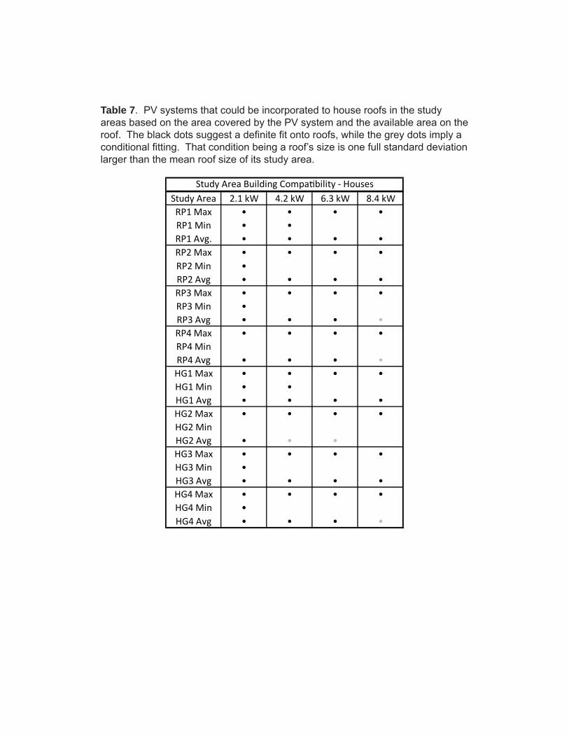
Table 7. PV systems that could be incorporated to house roofs in the study areas based on the area covered by the PV system and the available area on the roof. The black dots suggest a definite fit onto roofs, while the grey dots imply a conditional fitting. That condition being a roof’s size is one full standard deviation larger than the mean roof size of its study area.

Study Area 2.1 kW 4.2 kW 6.3 kW 8.4 kW

RP1 Max • • • •

RP1 Min • •

RP1 Avg. • • • •

RP2 Max • • • •

RP2 Min •

RP2 Avg • • • •

RP3 Max • • • •

RP3 Min •

RP3 Avg • • • •

RP4 Max • • • •

RP4 Min

RP4 Avg • • • •

HG1 Max • • • •

HG1 Min • •

HG1 Avg • • • •

HG2 Max • • • •

HG2 Min

HG2 Avg • • •

HG3 Max • • • •

HG3 Min •

HG3 Avg • • • •

HG4 Max • • • •

HG4 Min •

HG4 Avg • • • •

Study Area Building Compatibility - Houses

Table 8. PV systems that could be incorporated to garage roofs in the study areas based on the area covered by the PV system and the available area on the roof. The black dots suggest a definite fit onto roofs, while the grey dots imply a conditional fitting.

NA NA NA NA

Study Area Max Min Avg.

DT1 1800

DT2 685 335 510

DT3 600 95 345

DT4 195 10 95

Maximum System Based on Size (kW)

Table 9. Table that shows the maximum PV system size that could be imple-mented on a downtown study area roof.

Study Area 2.1 kW 4.2 kW 6.3 kW 8.4 kW

RP1 Max •

RP1 Min

RP1 Avg. •

RP2 Max •

RP2 Min

RP2 Avg •

RP3 Max •

RP3 Min

RP3 Avg

RP4 Max •

RP4 Min •

RP4 Avg •

HG1 Max • •

HG1 Min •

HG1 Avg • •

HG2 Max

HG2 Min

HG2 Avg

HG3 Max

HG3 Min

HG3 Avg

HG4 Max •

HG4 Min •

HG4 Avg •

Study Area Building Compatibility - Garages

37  

CHAPTER FOUR: CONCLUSIONS AND DISCUSSION

Based on the NDVI of the IKONOS image, there are many locations of sealed surfaces

that could accommodate the presence of PV systems. The NDVI also indicates that vegetation

does not affect the available roof area in the immediate vicinity of the buildings. Building roofs

are only a fraction of the surface area that could be employed to reduce the dependence of the

limited fuel sources that power West Virginia. Surfaces such as parking lots could be covered

by shading kiosks that are roofed in solar panels and reduce the amount of solar radiation that

would be absorbed by the concrete. This would keep cars cooler during intense summer days

as well as reduce the urban heat island effect caused by heated concrete and asphalt.

The majority of houses within the Huntington area are capable of supporting a 6.3 kW

system. The largest houses within the Ritter Park and Hal Greer study areas are capable of

supporting PV systems of 8.4 kW or larger. The smallest roofs of the residential areas were

able to accommodate, at most, 4.2 kW systems, but the majority can only support 2.1 kW

systems. The roof surfaces of the buildings in the Downtown study area were constructed flat,

ergo their entire surface could be used for any placement of a PV system. If a garage is present

and the house roof is not large enough to accommodate a system that provides full energy

autonomy, the garage roof may be used to include a smaller system that could increase the

amount of self-sufficiency. The maximum allowed 25 kW system could be used by farmers or

larger properties to supply energy to multiple buildings that use minimal energy as well as the

main dwelling where more power is required; however, they might produce impressive amounts

of excess energy and never fully use the credit attributed to them based on Appalachian

Power’s regulations.

According to this study, implementation of solar panels is possible to at least reduce

the amount of energy needed from a power company by 75%. Hypothetically, smaller houses

may use less power and the 6.3 kW system could supply the 100% independence ultimately

38  

sought, while larger houses may require a system with a higher energy production level, but

may have the area available to incorporate a larger system. If a grid connected system is used

with Appalachian Power, any excess power generated during the day is credited to the

homeowner and may reduce the cost of energy. The credited energy only lasts for 12 months;

however, that may provide ample time to use any of this energy during times of lower power

production (Appalachian Power Company, 2007). Any PV system used decreases the energy

demand peaks that occur throughout the day time hours. Though the demand peaks are

reduced with the use of a 2.1 kW system, production of surplus power does not occur until a 4.2

kW system or larger is put into use. The peaks that occur during the evening hours after the

sun has set can only be affected by solar panels if the energy created by a PV system is stored

in batteries or if the credit from power companies is used.

This project was meant to raise awareness of the options available to the Huntington,

West Virginia locale for the reduction of energy dependence based on finite resources. The

findings of this study indicate that a grid-connected PV system is not the ultimate answer to

power usage needs but would still prove highly beneficial. Although power companies are able

to produce a baseline of power throughout the day and import and export energy as needed

from other locations, grid-connected systems could reduce the baseline power production and

reduce the amount of natural resources needed to equal demand.

This pilot study could be expanded to include all buildings in the Huntington area that are

currently in use to gain better average building sizes. Resources that would benefit further

studies would be power data for residential use and for commercial/industrial use if it could be

retrieved either through donation from power companies or purchased through the use of

grants, up-to-date IKONOS, Digital Orthographic Quarter Quads, and SAMB images to

determine footprints and areas of newer buildings (such as locations like Pullman Square in

downtown Huntington), and finally, more accurate data about the number of households and

39  

businesses or corporations within the RFC to help determine a more correct average power

usage rate per hour. Other studies that could be derived from this research include the study of

other sealed surfaces, such as parking lots, for implementation of solar panel usage as

mentioned earlier. In addition, the amount of vacated buildings in the Huntington area that could

be converted into flat areas for the establishment of solar power production locations that may

reduce the city’s power usage costs could be evaluated.

The largest hindrance of PV systems is the initial cost to install the system. It will still be

many years before the PV cell becomes a more common tool for the reduction of non-

renewable source power production. Battery systems to store produced energy are also very

expensive and can increase the price of a PV system considerably. If all households were able

to produce 100% of their energy needs without including the use of batteries, large amounts of

surplus energy would be generated during daylight hours that could not be stored for later use.

For PV systems to be more feasible, battery prices and efficiencies need to be improved.

Increasing demand for PV cells would place emphasis on creating new PV production factories

that would increase production and decrease cost. The process to reduce cost could be

expedited by the use of tax cuts and purchase incentives.

One misconception of PV systems is that power companies would need to build

centralized PV power generation plants on large tracts of land, thus reducing the area allowed

for agricultural use. This study implies that PV systems can be decentralized and put into

service using the “wasted” surface area of roofs of buildings throughout a city.

Awareness needs to be raised about PV systems and other forms of renewable energy

sources. Increased familiarity would allow people to question current power production

methods as well as increase the understanding of the limits of natural resources. This would

40  

draw the interest of government backing to increase the amount of money returned through

incentives at the federal, state, and local levels.

41  

BIBLIOGRAPHY

Appalachian Power Company. Appalachian Power Company Fact Sheet. 2008.

Appalachian Power Company. West Virginia Net Metering Service Customer Information Packet. December, 2007.

Aratani, F., The Present Status and Future Direction of Technology Development for Photovoltaic Power Generation in Japan. Progress In Photovoltaics: Research and Applications, 2005; Vol 13: pp. 463-470.

BP Solar. Rebates and Incentives. <http://www.bp.com/extendedsectiongenericarticle.do?cate goryId=9019598&contentId=7036393>. March 3, 2009.

Canada, S., Moore, L., Post, H., and Strachan, J., Operation and Maintenance Field Experience for Off-grid Residential Photovoltaic Systems. Progress In Photovoltaics: Research and Applications, 2005; Vol 13: pp. 67-74.

Celik, A., Muneer, T., and Clarke, P., Optimal Sizing and Life Cycle Assessment of Residential Photovoltaic Energy Systems With Battery Storage. Progress In Photovoltaics: Research and Applications, 2008; Vol 16: pp. 69-85. 

Citizenrē Corporation. Forward Rental Agreement – General Terms and Conditions. December, 2007.

Citizenrē Corporation. <http://renu.citizenre.com/index.php?p=edu_solution>. April 10, 2009.

Cooler Planet. Solar Calculator. <http://solar.coolerplanet.com/Content/solar-calculator.aspx>. March 3, 2009.

Cooperative Networks For Renewable Resource Management. Bluefield State College Solar Irradiance Data. <http://rredc.nrel.gov/solar/new_data/confrrm/bs/>. July 18, 2008.

42  

Díaz, P., Egido, M., and Nieuwenhout, F., Dependability Analysis of Stand-Alone Photovoltaic Systems. Progress In Photovoltaics: Research and Applications, 2007; Vol 15: pp. 245-264.

Dunlop, E., and Halton, D., The Performance of Crystalline Silicon Photovoltaic Solar Modules after 22 Years of Continuous Outdoor Exposure. Progress In Photovoltaics: Research and Applications, 2006; Vol 14: pp. 53-64.

Energy Information Administration. Annual Energy Review. <http://www.eia.doe. gov/emeu/aer/pdf/pages/sec1_3.pdf>. 2007

Energy Information Administration. Energy Information Administration Energy Consumption Estimates by Source. 2006

Energy Information Administration. State data. <http://tonto.eia.doe.gov/state/>. March 3, 2009.

Find Solar. Solar Power Rating Map. <http://www.findsolar.com/Content/SolarPowerRating .aspx>. March 16, 2009.

Guha, S., and Yang, J., High-Efficiency Amorphous Silicon Alloy Based Solar Cells and Modules. National Renewable Energy Laboratory Subcontract Report. October, 2005. 130 pp.

Hahn, Giso, Solar Cells from Ribbon Silicon. Renewable Energy. Wegenmayr, R., Bϋhrke, T. (Eds.) Wiley-VCH Verlag GmbH & Co. 2008. pp 42-49.

Jensen, J.R., Introductory Digital Image Processing: A Remote Sensing Perspective. 3rd ed. Pearson Prentice Hall, 2005. 526 pp.

Jungbluth, N., Life Cycle Assessment of Crystalline Photovoltaics in the Swiss ecoinvent Database. Progress In Photovoltaics: Research and Applications, 2005; Vol 13: pp 429-446.

Komor, Paul, Renewable Energy Policy. iUniverse, Inc., 2004. 182 pp.

43 

Meyer, Nikolaus, Photovoltaic Cells on Glass. Renewable Energy. Wegenmayr, R., Bϋhrke, T. (Eds.) Wiley-VCH Verlag GmbH & Co. 2008. pp 50-53.

North American Electric Reliability Corporation. Councils Map. 2008.

Pitz-Paal, R., How the Sun gets into the Power Plant. Renewable Energy. Wegenmayr, R., Bϋhrke, T. (Eds.) Wiley-VCH Verlag GmbH & Co. 2008. pp 50-53.

Reliability First Corporation. Hourly Power Load Data. 2009.

Trishchenko, A., Cihlar, J., and Zhanqing, L., Effects of spectral response function on surface reflectance and NDVI measured with moderate resolution satellite sensors. Remote Sensing of Environment, 2002; Vol 81: pp. 1-18.

Twidell, J., and Weir, T., Renewable Energy Resources. 2nd ed. Taylor & Francis. 2006. 601 pp.

United States Census Bureau. TIGER/Line® 2000 Census Data Shapefiles. <http://www2. census.gov/cgi-bin/shapefiles/national-files>. March 4, 2009.

United States Department of Energy. Solar Energy Technologies Program. <http://www1.eere. energy.gov/solar/silicon.html>. April 28, 2009.

Wengenmayr, Roland, Solar Cells – an Overview. Renewable Energy. Wengenmayr, R., Bϋhrke, T. (Eds.) Wiley-VCH Verlag GmbH & Co. 2008. pp 34-40.

West Virginia State Legislature. Tax Exemption for Wind Energy Generation. West Virginia State Code § 11-13-2o. May, 2001.

Whitely, D.A., and Gallagher, T.R., Amended and Restated Delegation Agreement Between North American Electric Reliability Corporation and Reliability First Corporation. March 28, 2008. 15 pp.