a genetic algorithm for text classification rule induction - sci2s

A Genetic Algorithm for Text ClassificationRule Induction

Adriana Pietramala1, Veronica L. Policicchio1, Pasquale Rullo1,2,and Inderbir Sidhu3

1 University of Calabria Rende - Italy{a.pietramala,policicchio,rullo}@mat.unical.it

2 Exeura s.r.l. Rende, Italy3 Kenetica Ltd Chicago, IL-USA

[email protected]

Abstract. This paper presents a Genetic Algorithm, called Olex-GA,for the induction of rule-based text classifiers of the form “classify doc-ument d under category c if t1 ∈ d or ... or tn ∈ d and not (tn+1 ∈ dor ... or tn+m ∈ d) holds”, where each ti is a term. Olex-GA relies onan efficient several-rules-per-individual binary representation and usesthe F -measure as the fitness function. The proposed approach is testedover the standard test sets Reuters-21578 and Ohsumed and comparedagainst several classification algorithms (namely, Naive Bayes, Ripper,C4.5, SVM). Experimental results demonstrate that it achieves very goodperformance on both data collections, showing to be competitive with(and indeed outperforming in some cases) the evaluated classifiers.

1 Introduction

Text Classification is the task of assigning natural language texts to one or morethematic categories on the basis of their contents.

A number of machine learning methods have been proposed in the last fewyears, including k -nearest neighbors (k -NN), probabilistic Bayesian, neural net-works and SVMs. Overviews of these techniques can be found in [13, 20].

In a different line, rule learning algorithms, such as [2, 3, 18], have becomea successful strategy for classifier induction. Rule-based classifiers provide thedesirable property of being readable and, thus, easy for people to understand(and, possibly, modify).

Genetic Algorithms (GA’s) are stochastic search methods inspired to the bi-ological evolution [7, 14]. Their capability to provide good solutions for classicaloptimization tasks has been demonstrated by various applications, includingTSP [9, 17] and Knapsack [10]. Rule induction is also one of the applicationfields of GA’s [1, 5, 15, 16]. The basic idea is that each individual encodes acandidate solution (i.e., a classification rule or a classifier), and that its fitnessis evaluated in terms of predictive accuracy.

W. Daelemans et al. (Eds.): ECML PKDD 2008, Part II, LNAI 5212, pp. 188–203, 2008.c© Springer-Verlag Berlin Heidelberg 2008

A Genetic Algorithm for Text Classification Rule Induction 189

In this paper we address the problem of inducing propositional text classifiersof the form

c ← (t1 ∈ d ∨ · · · ∨ tn ∈ d) ∧ ¬(tn+1 ∈ d ∨ · · · ∨ tn+m ∈ d)

where c is a category, d a document and each ti a term (n-gram) taken from agiven vocabulary. We denote a classifier for c as above by Hc(Pos, Neg), wherePos = {t1, · · · , tn} and Neg = {tn+1 · · · tn+m}. Positive terms in Pos are used tocover the training set of c, while negative terms in Neg are used to take precisionunder control.

The problem of learning Hc(Pos, Neg) is formulated as an optimization task(hereafter referred to as MAX-F) aimed at finding the sets Pos and Neg whichmaximize the F -measure when Hc(Pos, Neg) is applied to the training set.MAX-F can be represented as a 0-1 combinatorial problem and, thus, the GA ap-proach turns out to be a natural candidate resolution method. We call Olex-GAthe genetic algorithm designed for the task of solving problem MAX-F.

Thanks to the simplicity of the hypothesis language, in Olex-GA an individ-ual represents a candidate classifier (instead of a single rule). The fitness of anindividual is expressed in terms of the F -measure attained by the correspond-ing classifier when applied to the training set. This several-rules-per-individualapproach (as opposed to the single-rule-per-individual approach) provides theadvantage that the fitness of an individual reliably indicates its quality, as it isa measure of the predictive accuracy of the encoded classifier rather than of asingle rule.

Once the population of individuals has been suitably initialized, evolutiontakes place by iterating elitism, selection, crossover and mutation, until a pre-defined number of generations is created.

Unlike other rule-based systems (such as Ripper) or decision tree systems(like C4.5) the proposed method is a one-step learning algorithm which doesnot need any post-induction optimization to refine the induced rule set. This isclearly a notable advantage, as rule set-refinement algorithms are rather complexand time-consuming tasks.

The experimentation over the standard test sets Reuters-21578 and Ohsu-

med confirms the goodness of the proposed approach: on both data collections,Olex-GA showed to be highly competitive with some of the top-performinglearning algorithms for text categorization, notably, Naive Bayes, C4.5, Ripperand SVM (both polynomial and rbf). Furthermore, it consistently defeated thegreedy approach to problem MAX-F we reported in [19]. In addition, Olex-GAturned out to be an efficient rule induction method (e.g., faster than both C4.5and Ripper).

In the rest of the paper, after providing a formulation of the learning op-timization problem (Section 2) and proving its NP-hardness, we describe theGA approach proposed to solve it (Section 3). Then, we present the experi-mental results (Section 5) and provide a performance comparison with some ofthe top-performing learning approaches (Section 6). Finally, we briefly discussthe relation to other rule induction systems (Sections 7 and 8) and give theconclusions.

190 A. Pietramala et al.

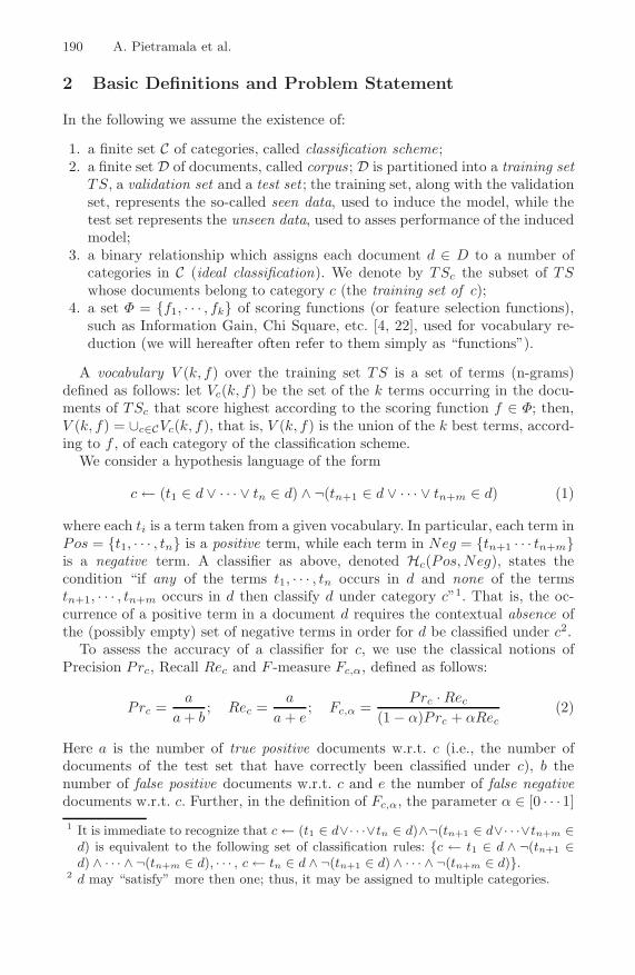
2 Basic Definitions and Problem Statement

In the following we assume the existence of:

1. a finite set C of categories, called classification scheme;2. a finite set D of documents, called corpus ; D is partitioned into a training set

TS, a validation set and a test set ; the training set, along with the validationset, represents the so-called seen data, used to induce the model, while thetest set represents the unseen data, used to asses performance of the inducedmodel;

3. a binary relationship which assigns each document d ∈ D to a number ofcategories in C (ideal classification). We denote by TSc the subset of TSwhose documents belong to category c (the training set of c);

4. a set Φ = {f1, · · · , fk} of scoring functions (or feature selection functions),such as Information Gain, Chi Square, etc. [4, 22], used for vocabulary re-duction (we will hereafter often refer to them simply as “functions”).

A vocabulary V (k, f) over the training set TS is a set of terms (n-grams)defined as follows: let Vc(k, f) be the set of the k terms occurring in the docu-ments of TSc that score highest according to the scoring function f ∈ Φ; then,V (k, f) = ∪c∈CVc(k, f), that is, V (k, f) is the union of the k best terms, accord-ing to f , of each category of the classification scheme.

We consider a hypothesis language of the form

c ← (t1 ∈ d ∨ · · · ∨ tn ∈ d) ∧ ¬(tn+1 ∈ d ∨ · · · ∨ tn+m ∈ d) (1)

where each ti is a term taken from a given vocabulary. In particular, each term inPos = {t1, · · · , tn} is a positive term, while each term in Neg = {tn+1 · · · tn+m}is a negative term. A classifier as above, denoted Hc(Pos, Neg), states thecondition “if any of the terms t1, · · · , tn occurs in d and none of the termstn+1, · · · , tn+m occurs in d then classify d under category c”1. That is, the oc-currence of a positive term in a document d requires the contextual absence ofthe (possibly empty) set of negative terms in order for d be classified under c2.

To assess the accuracy of a classifier for c, we use the classical notions ofPrecision Prc, Recall Rec and F -measure Fc,α, defined as follows:

Prc =a

a + b; Rec =

a

a + e; Fc,α =

Prc · Rec

(1 − α)Prc + αRec(2)

Here a is the number of true positive documents w.r.t. c (i.e., the number ofdocuments of the test set that have correctly been classified under c), b thenumber of false positive documents w.r.t. c and e the number of false negativedocuments w.r.t. c. Further, in the definition of Fc,α, the parameter α ∈ [0 · · · 1]

1 It is immediate to recognize that c ← (t1 ∈ d∨· · ·∨tn ∈ d)∧¬(tn+1 ∈ d∨· · ·∨tn+m ∈d) is equivalent to the following set of classification rules: {c ← t1 ∈ d ∧ ¬(tn+1 ∈d) ∧ · · · ∧ ¬(tn+m ∈ d), · · · , c ← tn ∈ d ∧ ¬(tn+1 ∈ d) ∧ · · · ∧ ¬(tn+m ∈ d)}.

2 d may “satisfy” more then one; thus, it may be assigned to multiple categories.


is the relative degree of importance given to Precision and Recall; notably, ifα = 1 then Fc,α coincides with Prc, and if α = 0 then Fc,α coincides with Rec

(a value of α = 0.5 attributes the same importance to Prc and Rec)3.Now we are in a position to state the following optimization problem:

PROBLEM MAX-F. Let a category c ∈ C and a vocabulary V (k, f) overthe training set TS be given. Then, find two subsets of V (k, f), namely, Pos ={t1, · · · , tn} and Neg = {tn+1, · · · , tn+m}, with Pos �= ∅, such that Hc(Pos, Neg)applied to TS yields a maximum value of Fc,α (over TS), for a given α.

Proposition 1. Problem MAX-F is NP-hard.

Proof. We next show that the decision version of problem MAX-F is NP-complete (i.e., it requires time exponential in the size of the vocabulary, unlessP = NP ). To this end, we restrict our attention to the subset of the hypothesislanguage where each rule consists of only positive terms, i.e, c ← t1 ∈ d∨· · ·∨tn ∈d (that is, classifiers are of the form Hc(Pos, ∅)). Let us call MAX-F+ this specialcase of problem MAX-F.

Given a generic set Pos ⊆ V (k, f), we denote by S ⊆ {1, · · · , p} the set ofindices of the elements of V (k, f) = {t1, · · · , tq} that are in Pos, and by Δ(ti)the set of documents of the training set TS where ti occurs. Thus, the set ofdocuments classifiable under c by Hc(Pos, ∅) is D(Pos) = ∪i∈SΔ(ti). The F -measure of this classification is

Fc,α(Pos) =|D(Pos) ∩ TSc|

(1 − α)|TSc| + α|D(Pos)| . (3)

Now, problem MAX-F+, in its decision version, can be formulated as follows:“∃ Pos ⊆ V (k, f) such that Fc,α(Pos) ≥ K?”, where K is a constant (let us callit MAX-F+(D)).

Membership. Since Pos ⊆ V (k, f), we can clearly verify a YES answer of MAX-F+(D), using equation 3, in time polynomial in the size |V (k, f)| of the vocab-ulary.

Hardness. We define a partition of D(Pos) into the following subsets: (1) Ψ(Pos)= D(Pos)∩TSc, i.e., the set of documents classifiable under c by Hc(Pos, ∅) thatbelong to the training set TSc (true classifiable); (2) Ω(Pos) = D(Pos) \ TSc,i.e., the set of documents classifiable under c by Hc(Pos, ∅) that do not belongto TSc (false classifiable).

Now, it is straightforward to see that the F -measure, given by equation 3, isproportional to the size ψ(Pos) of Ψ(Pos) and inversely proportional to the sizeω(Pos) of Ω(Pos) (just replace in equation 3 the quantities |D(Pos) ∩ TSc| byψ(Pos) and |D(Pos)| by ψ(Pos) + ω(Pos)). Therefore, problem MAX-F+(D)can equivalently be stated as follows: “∃ Pos ⊆ V (k, f) such that ψ(Pos) ≥ Vand ω(Pos) ≤ C?”, where V and C are constants.3 Since α ∈ [0 · · · 1] is a parameter of our model, we find convenient using Fc,α rather

than the equivalent Fβ = (β2+1)Prc·Rec

β2Prc+Rec, where β ∈ [0 · · · ∞] has no upper bound.


Now, let us restrict MAX-F+(D) to the simpler case in which terms in Posare pairwise disjoint, i.e., Δ(ti) ∩ Δ(tj) = ∅ for all ti, tj ∈ V (k, f) (let us callDSJ this assumption). Next we show that, under DSJ , MAX-F+(D) coincideswith the Knapsack problem. To this end, we associate with each ti ∈ V (k, f)two constants, vi (the value of ti) and a ci (the cost of ti) as follows:

vi = |Δ(ti) ∩ TSc|, ci = |Δ(ti) \ TSc|.

That is, the value vi (resp. cost ci) of a term ti is the number of documentscontaining ti that are true classifiable (resp., false classifiable).

Now we prove that, under DSJ , the equality Σi∈Svi = ψ(Pos) holds, for anyPos ⊆ V (k, f). Indeed:

Σi∈Svi = Σi∈S |Δ(ti)∩TSc| = |(∪i∈SΔ(ti))∩TSc| = |(D(Pos)∩TSc| = ψ(Pos).

To get the first equality above we apply the definition of vi; for the second, weexploit assumption DSJ ; for the third and the fourth we apply the definitionsof D(Pos) and ψ(Pos), respectively.

In the same way as for vi, the equality Σi∈Sci = ω(Pos) can be easily drawn.Therefore, by replacing ψ(Pos) and ω(Pos) in our decision problem, we get

the following new formulation, valid under DSJ : “∃ Pos ⊆ V (k, f) such thatΣi∈Svi ≥ V and Σi∈Sci ≤ C?”. That is, under DSJ , MAX-F+(D) is the Knap-sack problem – a well known NP-complete problem. Therefore, MAX-F+(D)under DSJ is NP-complete. It turns out that (the general case of) MAX-F+(D)(which is at least as complex as MAX-F+(D) under DSJ ) is NP-hard and, thus,the decision version of problem MAX-F+ is NP-hard as well. It turns out thatthe decision version of problem MAX-F is NP-hard.

Having proved both membership (in NP) and hardness, we conclude that thedecision version of problem MAX-F is NP-complete.

A solution of problem MAX-F is a best classifier for c over the training set TS,for a given vocabulary V (f, k). We assume that categories in C are mutuallyindependent, i.e., the classification results of a given category are not affectedby the results of any other. It turns out that we can solve problem MAX-F forthat category independently on the others. For this reason, in the following, wewill concentrate on a single category c ∈ C.

3 Olex-GA: A Genetic Algorithm to Solve MAX-F

Problem MAX-F is a combinatorial optimization problem aimed at finding abest combination of terms taken from a given vocabulary. That is, MAX-F isa typical problem for which GA’s are known to be a good candidate resolutionmethod.

A GA can be regarded as composed of three basic elements: (1) A population,i.e., a set of candidate solutions, called individuals or chromosomes, that willevolve during a number of iterations (generations); (2) a fitness function used to


assign a score to each individual of the population; (3) an evolution mechanismbased on operators such as selection, crossover and mutation. A comprehensivedescription of GA can be found in [7].

Next we describe our choices concerning the above points.

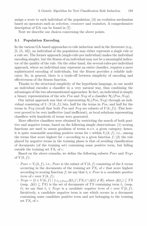
3.1 Population Encoding

In the various GA-based approaches to rule induction used in the literature (e.g.,[5, 15, 16]), an individual of the population may either represent a single rule ora rule set. The former approach (single-rule-per-individual) makes the individualencoding simpler, but the fitness of an individual may not be a meaningful indica-tor of the quality of the rule. On the other hand, the several-rules-per-individualapproach, where an individual may represent an entire classifier, requires a moresophisticated encoding of individuals, but the fitness provides a reliable indi-cator. So, in general, there is a trade-off between simplicity of encoding andeffectiveness of the fitness function.

Thanks to the structural simplicity of the hypothesis language, in our modelan individual encodes a classifier in a very natural way, thus combining theadvantages of the two aforementioned approaches. In fact, an individual is simplya binary representation of the sets Pos and Neg of a classifier Hc(Pos, Neg).

Our initial approach was that of representing Hc(Pos, Neg) through an indi-vidual consisting of 2 · |V (k, f)| bits, half for the terms in Pos, and half for theterms in Neg (recall that both Pos and Neg are subsets of V (k, f)). This how-ever proved to be very ineffective (and inefficient), as local solutions representingclassifiers with hundreds of terms were generated.

More effective classifiers were obtained by restricting the search of both posi-tive and negative terms, based on the following simple observations: (1) scoringfunctions are used to assess goodness of terms w.r.t. a given category; hence,it is quite reasonable searching positive terms for c within Vc(k, f), i.e., amongthe terms that score highest for c according to a given function f ; (2) the roleplayed by negative terms in the training phase is that of avoiding classificationof documents (of the training set) containing some positive term, but fallingoutside the training set TSc of c.

Based on the above remarks, we define the following subsets Pos∗ and Neg∗of V (k, f):

– Pos∗ = Vc(k, f), i.e., Pos∗ is the subset of V (k, f) consisting of the k termsoccurring in the documents of the training set TSc of c that score highestaccording to scoring function f ; we say that ti ∈ Pos∗ is a candidate positiveterm of c over V (k, f);

– Neg∗ = {t ∈ V (k, f) | (∪tj∈Pos∗Δ(tj)\TSc)∩Δ(t) �= ∅}, where Δ(tj) ⊆ TS(resp. Δ(t) ⊆ TS) is the set of documents of TS containing term tj (resp.t); we say that ti ∈ Neg∗ is a candidate negative term of c over V (k, f).Intuitively, a candidate negative term is one which occurs in a documentcontaining some candidate positive term and not belonging to the trainingset TSc of c.


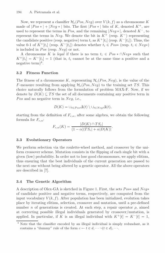
Now, we represent a classifier Hc(Pos, Neg) over V (k, f) as a chromosome Kmade of |Pos ∗ | + |Neg ∗ | bits. The first |Pos ∗ | bits of K, denoted K+, areused to represent the terms in Pos, and the remaining |Neg ∗ |, denoted K−, torepresent the terms in Neg. We denote the bit in K+ (resp. K−) representingthe candidate positive (resp. negative) term ti as K+[ti] (resp. K−[ti]). Thus, thevalue 0-1 of K+[ti] (resp. K−[ti]) denotes whether ti ∈ Pos∗ (resp. ti ∈ Neg∗)is included in Pos (resp. Neg) or not.

A chromosome K is legal if there is no term ti ∈ Pos ∗ ∩Neg∗ such thatK+[ti] = K−[ti] = 1 (that is, ti cannot be at the same time a positive and anegative term)4.

3.2 Fitness Function

The fitness of a chromosome K, representing Hc(Pos, Neg), is the value of theF -measure resulting from applying Hc(Pos, Neg) to the training set TS. Thischoice naturally follows from the formulation of problem MAX-F. Now, if wedenote by D(K) ⊆ TS the set of all documents containing any positive term inPos and no negative term in Neg, i.e.,

D(K) = ∪t∈PosΔ(t) \ ∪t∈NegΔ(t),

starting from the definition of Fc,α, after some algebra, we obtain the followingformula for Fc,α:

Fc,α(K) =|D(K) ∩ TSc|

(1 − α)|TSc| + α|D(K)| .

3.3 Evolutionary Operators

We perform selection via the roulette-wheel method, and crossover by the uni-form crossover scheme. Mutation consists in the flipping of each single bit with agiven (low) probability. In order not to lose good chromosomes, we apply elitism,thus ensuring that the best individuals of the current generation are passed tothe next one without being altered by a genetic operator. All the above operatorsare described in [7].

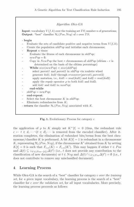
3.4 The Genetic Algorithm

A description of Olex-GA is sketched in Figure 1. First, the sets Pos∗ and Neg∗of candidate positive and negative terms, respectively, are computed from theinput vocabulary V (k, f). After population has been initialized, evolution takesplace by iterating elitism, selection, crossover and mutation, until a pre-definednumber n of generations is created. At each step, a repair operator ρ, aimedat correcting possible illegal individuals generated by crossover/mutation, isapplied. In particular, if K is an illegal individual with K+[t] = K−[t] = 1,4 Note that the classifier encoded by an illegal individual is simply redundant, as it

contains a “dummy” rule of the form c ← t ∈ d, · · · ¬(t ∈ d), · · ·.


Algorithm Olex-GA

Input: vocabulary V (f, k) over the training set TS; number n of generations;Output: “best” classifier Hc(Pos,Neg) of c over TS;

- begin- Evaluate the sets of candidate positive and negative terms from V (f, k);- Create the population oldPop and initialize each chromosome;- Repeat n times- Evaluate the fitness of each chromosome in oldPop;- newPop = ∅;- Copy in NewPop the best r chromosomes of oldPop (elitism - r is

determined on the basis of the elitism percentage)- While size(newPop) < size(oldPop)- select parent1 and parent2 in oldPop via roulette wheel- generate kid1, kid2 through crossover(parent1, parent2)- apply mutation, i.e., kid1 = mut(kid1) and kid2 = mut(kid2)- apply the repair operator ρ to both kid1 and kid2;- add kid1 and kid2 to newPop;- end-while- oldPop = newPop;- end-repeat;- Select the best chromosome K in oldPop;- Eliminate redundancies from K;- return the classifier Hc(Pos,Neg) associated with K.

Fig. 1. Evolutionary Process for category c

the application of ρ to K simply set K+[t] = 0 (thus, the redundant rulec ← t ∈ d, · · · ¬(t ∈ d), · · · is removed from the encoded classifier). After it-eration completes, the elimination of redundant bits/terms from the best chro-mosome/classifier K is performed. A bit K[t] = 1 is redundant in a chromosomeK, representing Hc(Pos, Neg), if the chromosome K ′ obtained from K by settingK[t] = 0 is such that Fc,α(K) = Fc,α(K ′). This may happen if either t ∈ Posand Δ(t) ⊆ ∪t′∈(Pos−{t})Δ(t′) (i.e., t does not provide any contribution to theclassification of new documents) or t ∈ Neg and Δ(t) ∩ ∪t′∈PosΔ(t′) = ∅ (i.e., tdoes not contribute to remove any misclassified document).

4 Learning Process

While Olex-GA is the search of a “best” classifier for category c over the trainingset, for a given input vocabulary, the learning process is the search of a “best”classifier for c over the validation set, for all input vocabularies. More precisely,the learning process proceeds as follows:


– Learning: for each input vocabulary• Evolutionary Process: execute a predefined number of runs of Olex-GA

over the training set, according to Figure 1;• Validation: run over the validation set the best chromosome/classifier

generated by Olex-GA;– Testing: After all runs have been executed, pick up the best classifier (over

the validation set), and assess its accuracy over the test set (unseen data).

The output of the learning process is assumed to be the “best classifier” of c.

5 Experimentation

5.1 Benchmark Corpora

We have experimentally evaluated our method using both the Reuters-21578

[12] and and the Ohsumed [8] test collections.The Reuters-21578 consists of 12,902 documents. We have used the Mod-

Apte split, in which 9,603 documents are selected for training (seen data) andthe other 3,299 form the test set (unseen data). Of the 135 categories of theTOPICS group, we have considered the 10 with the highest number of positivetraining examples (in the following, we will refer to this subset as R10). Weremark that we used all 9603 documents of the training corpus for the learningphase, and performed the test using all 3299 documents of the test set (includingthose not belonging to any category in R10).

The second data set we considered is Ohsumed, in particular, the collectionconsisting of the first 20,000 documents from the 50,216 medical abstracts ofthe year 1991. Of the 20,000 documents of the corpus, the first 10,000 were usedas seen data and the second 10,000 as unseen data. The classification schemeconsisted of the 23 MeSH diseases.

5.2 Document Pre-processing

Preliminarily, documents were subjected to the following pre-processing steps:(1) First, we removed all words occurring in a list of common stopwords, as wellas punctuation marks and numbers; (2) then, we extracted all n-grams, definedas sequences of maximum three words consecutively occurring within a document(after stopword removal)5; (3) at this point we have randomly split the set ofseen data into a training set (70%), on which to run the GA, and a validation set(30%), on which tuning the model parameters. We performed the split in sucha way that each category was proportionally represented in both sets (stratifiedholdout); (4) finally, for each category c ∈ C, we scored all n-grams occurring inthe documents of the training set TSc by each scoring function f ∈ {CHI, IG},where IG stands for Information Gain and CHI for Chi Square [4, 22].

5 Preliminary experiments showed that n-grams of length ranging between 1 and 3perform slightly better than single words.


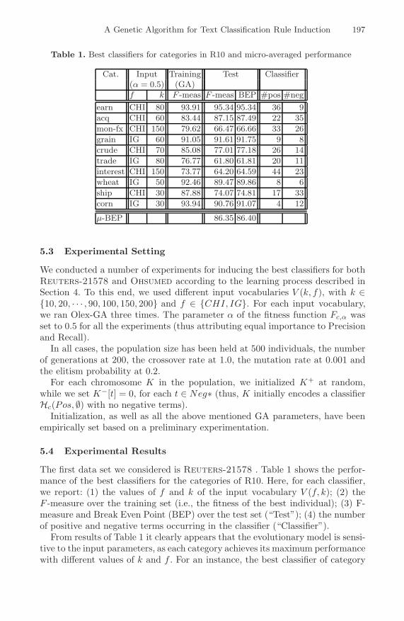
Table 1. Best classifiers for categories in R10 and micro-averaged performance

Cat. Input Training Test Classifier(α = 0.5) (GA)f k F -meas F -meas BEP #pos #neg

earn CHI 80 93.91 95.34 95.34 36 9acq CHI 60 83.44 87.15 87.49 22 35mon-fx CHI 150 79.62 66.47 66.66 33 26grain IG 60 91.05 91.61 91.75 9 8crude CHI 70 85.08 77.01 77.18 26 14trade IG 80 76.77 61.80 61.81 20 11interest CHI 150 73.77 64.20 64.59 44 23wheat IG 50 92.46 89.47 89.86 8 6ship CHI 30 87.88 74.07 74.81 17 33corn IG 30 93.94 90.76 91.07 4 12

μ-BEP 86.35 86.40

5.3 Experimental Setting

We conducted a number of experiments for inducing the best classifiers for bothReuters-21578 and Ohsumed according to the learning process described inSection 4. To this end, we used different input vocabularies V (k, f), with k ∈{10, 20, · · · , 90, 100, 150, 200} and f ∈ {CHI, IG}. For each input vocabulary,we ran Olex-GA three times. The parameter α of the fitness function Fc,α wasset to 0.5 for all the experiments (thus attributing equal importance to Precisionand Recall).

In all cases, the population size has been held at 500 individuals, the numberof generations at 200, the crossover rate at 1.0, the mutation rate at 0.001 andthe elitism probability at 0.2.

For each chromosome K in the population, we initialized K+ at random,while we set K−[t] = 0, for each t ∈ Neg∗ (thus, K initially encodes a classifierHc(Pos, ∅) with no negative terms).

Initialization, as well as all the above mentioned GA parameters, have beenempirically set based on a preliminary experimentation.

5.4 Experimental Results

The first data set we considered is Reuters-21578 . Table 1 shows the perfor-mance of the best classifiers for the categories of R10. Here, for each classifier,we report: (1) the values of f and k of the input vocabulary V (f, k); (2) theF -measure over the training set (i.e., the fitness of the best individual); (3) F-measure and Break Even Point (BEP) over the test set (“Test”); (4) the numberof positive and negative terms occurring in the classifier (“Classifier”).

From results of Table 1 it clearly appears that the evolutionary model is sensi-tive to the input parameters, as each category achieves its maximum performancewith different values of k and f . For an instance, the best classifier of category


“earn” is learned from a vocabulary V (k, f) where k = 80 and f = CHI; therespective F -measure and breakeven point are both 95.34. Looking at the lastrow, we see that the micro-averaged values of F -measure and BEP over thetest set are equal to 86.35 and 86.40, respectively. Finally, looking at the lasttwo columns labelled “classifier”, we see that the induced classifiers are rathercompact: the maximum number of positive terms is 44 (“interest”), and theminimum is 4 (“corn”); likewise, the maximum number of negative terms is 35(“acq”) and the minimum is 6 (“wheat”).

As an example, the classifier Hc(Pos, Neg) for “corn” has

Pos = {“corn”, “maize”, “tonnes maize”, “tonnes corn”}

Neg = {“jan”, “qtr”, “central bank”, “profit”, “4th”, “bonds”, “pact”,

“offering”, “monetary”, “international”, “money”, “petroleum”}.

Thus, Hc(Pos, Neg) is of the following form:

c ← “corn” ∨ · · · ∨ “tonnes corn” ∧ ¬ (“jan” ∨ · · · ∨ “petroleum”).

To show the sensitivity of the model to parameter settings, in Table 2 wereport the F-measure values (on the validation set) for category “corn” obtainedby using different values for φ and ν. As we can see, the performance of theinduced classifiers varies from a minimum of 84.91 to a maximum of 93.58 (notethat, for both functions, the F -measure starts decreasing for ν > 50, i.e., areduction of the vocabulary size provides a benefit in terms of performance [22]).

Table 2. Effect of varying φ and ν on the F-measure for category “corn”

ν

φ 10 50 100 150 200CHI 90.74 91.00 88.7 88.68 84.91IG 92.04 93.58 91.59 91.59 89.09

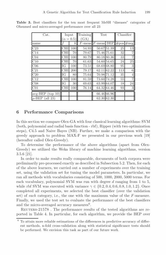
The second data set we considered is Ohsumed . In Table 3 we provide thebest performance for the ten most frequent Mesh categories and micro-averagedperformance over all 23. In particular, micro-averaged F -measure and BEP (overthe test set) are both equal to 62.30. Also in this case, with a few exceptions,classifiers are rather compact.

5.5 Time Efficiency

Experiments have been run on a 2.33 GHz Xeon 4 Gb RAM. The average ex-ecution time of the evolutionary process of Figure 1 is around 10 seconds percategory for both data sets (recall that in both cases the population is made of500 individuals which evolve for 200 generations).


Table 3. Best classifiers for the ten most frequent MeSH “diseases” categories ofOhsumed and micro-averaged performance over all 23

Cat. Input Training Test Classifier(α = 0.5) (GA)

name f k F -meas F -meas BEP #pos #negC23 CHI 100 54.93 50.67 51.39 25 13C14 CHI 70 79.67 75.46 75.61 32 7C04 CHI 100 80.79 80.18 80.36 33 7C10 CHI 70 61.63 54.60 54.65 24 25C06 IG 100 73.51 68.69 68.80 95 3C21 CHI 200 79.17 62.11 62.22 113 6C20 IG 80 75.64 70.98 71.12 35 4C12 CHI 100 81.59 73.60 74.28 55 7C08 IG 30 69.63 63.99 64.07 18 24C01 CHI 100 76.14 64.32 64.46 93 3

avg-BEP (top 10) 66.46 66.96μ-BEP (all 23) 62.30 62.30

6 Performance Comparisons

In this section we compare Olex-GA with four classical learning algorithms: SVM(both, polynomial and radial basis function - rbf), Ripper (with two optimizationsteps), C4.5 and Naive Bayes (NB). Further, we make a comparison with thegreedy approach to problem MAX-F we presented in our previous work [19](hereafter called Olex-Greedy).

To determine the performance of the above algorithms (apart from Olex-Greedy) we utilized the Weka library of machine learning algorithms, version3.5.6 [21].

In order to make results really comparable, documents of both corpora werepreliminarily pre-processed exactly as described in Subsection 5.2. Then, for eachof the above learners, we carried out a number of experiments over the trainingset, using the validation set for tuning the model parameters. In particular, weran all methods with vocabularies consisting of 500, 1000, 2000, 5000 terms. Foreach vocabulary, polynomial SVM was run with degree d ranging from 1 to 5,while rbf SVM was executed with variance γ ∈ {0.2, 0.4, 0.6, 0.8, 1.0, 1.2}. Oncecompleted all experiments, we selected the best classifier (over the validationset) of each category, i.e., the one with the maximum value of the F -measure.Finally, we used the test set to evaluate the performance of the best classifiersand the micro-averaged accuracy measures6.

Reuters-21578 . The performance results of the tested algorithms are re-ported in Table 4. In particular, for each algorithm, we provide the BEP over6 To attain more reliable estimations of the differences in predictive accuracy of differ-

ent methods, n-fold cross-validation along with statistical significance tests shouldbe performed. We envision this task as part of our future work.


Table 4. Recall/Precision breakeven points on R10

Category NB C4.5 Ripper SVM Olexpoly rbf Greedy GA

earn 96.61 95.77 95.31 97.32 96.57 93.13 95.34acq 90.29 85.59 86.63 90.37 90.83 84.32 87.49money 56.67 63.08 62.94 72.89 68.22 68.01 66.66grain 77.82 89.69 89.93 92.47 88.94 91.28 91.75crude 78.84 82.43 81.07 87.82 86.17 80.84 77.18trade 57.90 70.04 75.82 77.77 74.14 64.28 61.81interest 61.71 52.93 63.15 68.16 58.71 55.96 64.59wheat 71.77 91.46 90.66 86.13 89.25 91.46 89.86ship 68.65 71.92 75.91 82.66 80.40 78.49 74.81corn 59.41 86.73 91.79 87.16 84.74 89.38 91.07μ-BEP 82.52 85.82 86.71 89.91 88.80 84.80 86.40learning times (min) 0.02 425 800 46 696 2.30 116

the test set of each category in R10, the micro-avg BEP and the overall learningtime. Concerning predictive accuracy, with a μ-BEP of 86.40, our method sur-passes Naive Bayes (82.52), which shows the worst behavior, and Olex-Greedy(84.80); is competitive with C4.5 (85.82) and Ripper (86.71), while performsworse than both SVM’s (poly = 89.91, rbf = 88.80). Concerning efficiency, NB(0.02 min) and Olex-Greedy (2.30 min) are by far the fastest methods. Thenpoly SVM (46 min) and Olex-GA (116 min), followed at some distance by C4.5(425 min), rbf SVM (696 min) and Ripper (800).

Ohsumed . As we can see from Table 5, with a μ-BEP = 62.30, the proposedmethod is the top-performer. On the other side, C4.5 shows to be the worst

Table 5. Recall/Precision breakeven points on the ten most frequent MeSH diseasescategories of Ohsumed and micro-averaged performance over all 23

Category NB C4.5 Ripper SVM Olexpoly rbf Greedy GA

C23 47.59 41.93 35.01 45.00 44.21 47.32 51.39C14 77.15 73.79 74.16 73.81 75.34 74.52 75.61C04 75.71 76.22 80.05 78.18 76.65 77.78 80.36C10 45.96 44.88 49.73 52.22 51.54 54.72 54.65C06 65.19 57.47 64.99 63.18 65.10 63.25 68.80C21 54.92 61.68 61.42 64.95 62.59 61.62 62.22C20 68.09 64.72 71.99 70.23 66.39 67.81 71.12C12 63.04 65.42 70.06 72.29 64.78 67.82 74.28C08 57.70 54.29 63.86 60.40 55.33 61.57 64.07C01 58.36 48.89 56.05 43.05 52.09 55.59 64.46avg-BEP (top 10) 61.37 58.92 62.73 62.33 61.40 62.08 66.69μ-BEP (all 23) 57.75 55.14 59.65 60.24 59.57 59.38 62.30learning times (min) 0.04 805 1615 89 1100 6 249


performer (55.14) (so confirming the findings of [11]). Then, in the order, NaiveBayes (57.75), rbf SVM (59.57), Ripper (59.65), polynomial SVM (60.24) andOlex-Greedy (61.57). As for time efficiency, the Ohsumed results essentiallyconfirm the hierarchy coming out from the Reuters-21578 .

7 Olex-GA vs. Olex-Greedy

One point that is noteworthy is the relationship between Olex-Greedy and Olex-GA, in terms of both predictive accuracy and time efficiency.

Concerning the former, we have seen that Olex-GA consistently beats Olex-Greedy on both data sets. This confirms Freitas’ findings [6], according towhich effectiveness of GA’s in rule induction is a consequence of their inher-ent ability to cope with attribute interaction as, thanks to their global searchapproach, more attributes at a time are modified and evaluated as a whole.This in contrast with the local, one-condition-at-a-time greedy rule generationapproach.

On the other hand, concerning time efficiency, Olex-Greedy showed to be muchfaster than Olex-GA. This should not be surprising, as the greedy approach,unlike GA’s, provides a search strategy which straight leads to a suboptimalsolution.

8 Relation to Other Inductive Rule Learners

Because of the computational complexity of the learning problem, all real sys-tems employ heuristic search strategies which prunes vast parts of the hypothe-sis space. Conventional inductive rule learners (e.g, RIPPER [3]) usually adopt,as their general search method, a covering approach based on a separate-and-conquer strategy. Starting from an empty rule set, they learn a set of rules, oneby one. Different learners essentially differ in how they find a single rule. In RIP-PER, the construction of a single rule is a two-stage process: a greedy heuristicsconstructs an initial rule set (IREP*) and, then, one or more optimization phasesimprove compactness and accuracy of the rule set.

Also decision tree techniques, e.g., C4.5 [18], rely on a two-stage process. Afterthe decision tree has been transformed into a rule set, C4.5 implements a pruningstage which requires more steps to produce the final rule set - a rather complexand time consuming task.

In contrast, Olex-GA, like Olex-Greedy and other GA-based approaches (e.g.,[5]), relies on a single-step process whereby an “optimal” classifier, i.e., oneconsisting of few high-quality rules, is learned. Thus, no pruning strategy isneeded, with a great advantage in terms of efficiency. This may actually accountfor the time results of Tables 4 and 5, which show the superiority of Olex-GAw.r.t. both C4.5 and Ripper.


9 Conclusions

We have presented a Genetic Algorithm, Olex-GA, for inducing rule-based textclassifiers of the form ”if a document d includes either term t1 or ... or term tn,but not term tn+1 and ... and not term tn+m, then classify d under category c”.

Olex-GA relies on a simple binary representation of classifiers (several-rules-per-individual approach) and uses the F -measure as the fitness function. Onedesign aspect related to the encoding of a classifier Hc(Pos, Neg) was concernedwith the choice of the length of individuals (i.e., the size of the search space).Based on preliminary experiments, we have restricted the search of Pos and Negto suitable subsets of the vocabulary (instead of taking it entirely), thus gettingmore effective and compact classifiers.

The experimental results obtained on the standard data collections Reuters-

21578 and Ohsumed show that Olex-GA quickly converges to very accurateclassifiers. In particular, in the case of Ohsumed , it defeats all the other eval-uated algorithms. Further, on both data sets, Olex-GA consistently beats Olex-Greedy. As for time efficiency, Olex-GA is slower than Olex-Greedy but fasterthan the other rule learning methods (i.e., Ripper and C4.5).

We conclude by remarking that we consider the experiments reported in thispaper somewhat preliminary, and feel that performance can further be improvedthrough a fine-tuning of the GA parameters.

References

1. Alvarez, J.L., Mata, J., Riquelme, J.C.: Cg03: An oblique classification systemusing an evolutionary algorithm and c4.5. International Journal of Computer, Sys-tems and Signals 2(1), 1–15 (2001)

2. Apte, C., Damerau, F.J., Weiss, S.M.: Automated learning of decision rules for textcategorization. ACM Transactions on Information Systems 12(3), 233–251 (1994)

3. Cohen, W.W., Singer, Y.: Context-sensitive learning methods for text categoriza-tion. ACM Transactions on Information Systems 17(2), 141–173 (1999)

4. Forman, G.: An extensive empirical study of feature selection metrics for textclassification. Journal of Machine Learning Research 3, 1289–1305 (2003)

5. Freitas, A.A.: A genetic algorithm for generalized rule induction. In: Advances inSoft Computing-Engineering Design and Manufacturing, pp. 340–353. Springer,Heidelberg (1999)

6. Freitas, A.A.: In: Klosgen, W., Zytkow, J. (eds.) Handbook of Data Mining andKnowledge Discovery, ch. 32, pp. 698–706. Oxford University Press, Oxford (2002)

7. Goldberg, D.E.: Genetic Algorithms in Search, Optimization and Machine Learn-ing. Addison-Wesley, Reading (1989)

8. Hersh, W., Buckley, C., Leone, T., Hickman, D.: Ohsumed: an interactive retrievalevaluation and new large text collection for research. In: Croft, W.B., van Rijsber-gen, C.J. (eds.) Proceedings of SIGIR-1994, 17th ACM International Conferenceon Research and Development in Information Retrieval, Dublin, IE, pp. 192–201.Springer, Heidelberg (1994)

9. Homaifar, A., Guan, S., Liepins, G.E.: Schema analysis of the traveling salesmanproblem using genetic algorithms. Complex Systems 6(2), 183–217 (1992)


10. Hristakeva, M., Shrestha, D.: Solving the 0/1 Knapsack Problem with GeneticAlgorithms. In: Midwest Instruction and Computing Symposium 2004 Proceedings(2004)

11. Joachims, T.: Text categorization with support vector machines: learning withmany relevant features. In: Nedellec, C., Rouveirol, C. (eds.) ECML 1998. LNCS,vol. 1398, pp. 137–142. Springer, Heidelberg (1998)

12. Lewis, D.D.: Reuters-21578 text categorization test collection. Distribution 1.0(1997)

13. Lewis, D.D., Hayes, P.J.: Guest editors’ introduction to the special issue on textcategorization. ACM Transactions on Information Systems 12(3), 231 (1994)

14. Michalewicz, Z.: Genetic Algorithms+Data Structures=Evolution Programs, 3rdedn. Springer, Heidelberg (1999)

15. Noda, E., Freitas, A.A., Lopes, H.S.: Discovering interesting prediction rules with agenetic algorithm. In: Proc. Congress on Evolutionary Computation (CEC-1999),July 1999. IEEE, Washington (1999)

16. Pei, M., Goodman, E.D., Punch, W.F.: Pattern discovery from data using geneticalgorithms. In: Proc. 1st Pacific-Asia Conf. Knowledge Discovery and Data Mining(PAKDD-1997), Febuary 1997. World Scientific, Singapore (1997)

17. Jung, Y., Jog, S.P., van Gucht, D.: Parallel genetic algorithms applied to thetraveling salesman problem. SIAM Journal of Optimization 1(4), 515–529 (1991)

18. Quinlan, J.R.: Generating production rules from decision trees. In: Proc. of IJCAI-1987, pp. 304–307 (1987)

19. Rullo, P., Cumbo, C., Policicchio, V.L.: Learning rules with negation for text cat-egorization. In: Proc. of SAC - Symposium on Applied Computing, Seoul, Korea,March 11-15 2007, pp. 409–416. ACM, New York (2007)

20. Sebastiani, F.: Machine learning in automated text categorization. ACM Comput-ing Surveys 34(1), 1–47 (2002)

21. Witten, I.H., Frank, E.: Data Mining: Practical machine learning tools and tech-niques, 2nd edn. Morgan Kaufmann, San Francisco (2005)

22. Yang, Y., Pedersen, J.O.: A comparative study on feature selection in text cat-egorization. In: Fisher, D.H. (ed.) Proceedings of ICML-97, 14th InternationalConference on Machine Learning, Nashville, US, pp. 412–420. Morgan KaufmannPublishers, San Francisco (1997)

a genetic algorithm for text classification rule induction - sci2s

Documents