a generai-purpose contact detection algorithm for...

RECORD copy c1 l

SANDIA REPORT SAND92–2141 l UC–705 Unlimited Release Printed May 1993

A GeneraI-Purpose Contact Detection Algorithm for Nonlinear Structural Analysis Codes

M. W. Heinstein, S. W. Attaway, J. W. Swede, F. J. Mello -- ‘-- - “--’-

Prepared by Sandia National Laboratories Albuquerque, New Mexico 87185 and Livermore, California 94550 for the United States Department of Energy

II I I I I 1111 II II I I II under Contract DE-AC04-76DP00789

*8573079*

SANDIA NATIONAL LABORATORIES

TECHNICAL LIBRARY

SF2900Q(8-81)

Issued by Sandia National Laboratories, operated for the United States Department of Energy by Sandia Corporation. NOTICE This report was prepared as an account of work sponsored by an agency of the United States Government. Neither the United States Govern- ment nor any agency thereof, nor any of their employees, nor any of their contractors, subcontractors, or their employees, makes any warranty, express or implied, or assumes any legal liability or responsibility for the accuracy, completeness, or usefulness of any information, apparatus: product, or process disclosed, or represents that its use would not infringe privately owned rights. Reference herein to any specific commercial product, process, or service by trade name, trademark, manufacturer, or otherwise, does not necessarily constitute or imply its endorsement, recommendation, or favoring by the United States Government, any agency thereof or any of their contractors or subcontracts. The views and opinions expressed herein do not necessarily state or reflect those of the United States Government, any agency thereof or any of their contractors.

Printed in the United States of America. This report has been reproduced directly from the best available copy.

Available to DOE and DOE contractors from Office of Scientific and Technical Information PO BOX 62 Oak Ridge, TN 37831

Prices available from (615) 576-8401, FTX 626-8401

Available to the public from National Technical Information Service US Department of Commerce 5285 Port Royal Rd Springfield, VA 22161

NTIS price codes Printed copy A05 Microfiche copy AO1

SAND92-2141 Unlimited Release Printed May 1993

Distribution Category UC-705

A General-Purpose Contact Detection Algorithm for Nonlinear Structural Analysis Codes*

M.W. Heinstein Engineering Mechanics and Material Modeling Department

S.W. Attaway Computational Mechanics and Visualization Department

J.W. Swegle Experimental Impact Physics Department

F.J. Mello Solid and Structural Mechanics Department

Sandia National Laboratories Albuquerque, New Mexico 87185

Abstract

A new contact detection algorithm has been developed to address difficulties associated with the numerical simulation of contact in nonlinear finite element structural analysis codes. Problems including accurate and efficient detection of contact for self-contacting surfaces, tearing and eroding surfaces, and multi-body impact are addressed. The proposed algorithm is portable between dynamic and quasi-static codes and can efficiently model contact between a variety of finite element types including shells, bricks, beams and particles. The algorithm is composed of ( 1 ) a location strategy that uses a global search to decide which slave nodes are in proximity to a master surface and (2) an accurate detailed contact check that uses the projected motions of both master surface and slave node. In this report, currently used contact detection algorithms and their associated difficulties are discussed. Then the proposed algorithm and how it addresses these problems is described. Finally, the capability of the new algorithm is illustrated with several example problems.

* This work performed at Sandia National Laboratories supported by the U.S. Department of Energy under contract DE-AC04-76DP00789

1

Nomenclature

c

am, dt Ix, Iy, Iz iboxmin

iboxmm

jboxmin

jboxmm

kboxmin

kboxmm

(J)mi”

(ix-m=

(iy)min

lbox m

incremental time to contact

local surface coordinates of contact point

; component of surface normal

bucket containing node i

j component of surface normal bucket size number of slave node-master nodes comparisons made in 3D bucket

sorting

~ component of surface normal

vector from master surface node to slave node

current time step Index vector for the x, y, and z coordinate respectively slice of data containing minimum x-coordinate of master surface

capture box slice of data containing (maximum x-coordinate of master surface

capture box j

slice of data containing minimum y-coordinate of master surface capture box

slice of data containing maximum y-coordinate of master surface capture box

slice of data containing minimum z-coordinate of master surface capture box

slice of data containing maximum z-coordinate of master surface capture box

pointer into the Index vector corresponding to the first slave node inside a master surface capture box along the x-coordinate

pointer into the Index vector corresponding to the last slave node inside a master surface capture box along the x-coordinate

pointer into the Index vector corresponding to the f~st slave node inside a master surface capture box along the y-coordinate

pointer into the Index vector corresponding to the last slave node inside a master surface capture box along the y-coordinate

pointer into the Index vector corresponding to the first slave node inside a master surface capture box along the z-coordinate

pointer into the Index vector corresponding to the last slave node inside a master surface capture box along the z-coordinate

number of slave nodes in each bucket number of master nodes

2

A

‘P

N,n

n

ii nb

nbox ndsort npoint

h

P RX, RY, RZ

Sx, Sy, Sz

Vx,vy,vz

(vx~max

(Vyhnax

(Vz)max

‘i* Yi9zi9

“min

“m,ax YCmin

Ycm,nx ZCmin

Zcmm

number of master surfaces

unit normal of a master surface

unit normal of master surface i

unit normal of master surface at end of previous time step

surface normal of master surface

number of slave nodes

unit normal of the slave surface at a slave node total number of buckets bucket id for each slave node list of slave nodes sorted by ascending bucket id pointer into vector ndsort giving the starting location of the slave nodes

in each bucket

unit push-back direction at time t

penetration of slave node into master surface Rank vector for the x, y, and z coordinate respectively

number of slices required along the x, y and z coordinates respectively

slice along x, y and z coordinate containing node i

current time

velocity vector

velocity of slave node

velocity of master surface at contact point

x, y and z component of velocity

maximum x-component of velocity

maximum y-component of velocity

maximum z-component of velocity

x,y, and z coordinate of master surface nodal point i minimum x-coordinate of master surface capture box

maximum x-coordinate of master surface capture box minimum y-coordinate of master surface capture box

maximum y-coordinate of master surface capture box minimum z-coordinate of master surface capture box maximum z-coordinate of master surface capture box

Table of Contents

1. Introduction ..................................................................................................................7

2. Survey of Contact Detection Algorithms and Motivation for Current Work ........8

2.1 Neighborhood Identification ...................................................................................9

2.1.1 Surface Side-Set Pairing ..................................................................................... 10

2.1.2 Surface Tracting .................................................................................................lO

2.1.3 Bucket Seuching ................................................................................................l 1

2.1.4 Pinball Contact ....................................................................................................l2

2.2 Detailed Contact Check ......................................................................................... 13

2.2.1 Ideal Contact Determination ...............................................................................l3

2.2.2 Pushback inaccuracies ........................................................................................l4

2.2.3 Overdetermined Contact .....................................................................................l4

2.2.4 Undetermined Contact ........................................................................................l6

2.3 Motivation for Current Work .................................................................................l7

3. New Contact DetectionAlgorithm ............................................................................l93.1 New Neighborhood Identification Sna@gy ...........................................................l9

3.1.1 Algorithm for vector architecture .......................................................................l9

3.1.2 Algorithm for parallel architecture .....................................................................24

3.2 New Detailed Contact Check .................................................................................29

3.2.1 Velocity Based Contact Check ...........................................................................29

3.2.2 Static Contact Check ...........................................................................................32

3.3 Summary of New Contact Detection Algorithm ...................................................33

4. Surface Definition Algorithm .....................................................................................35

5. Example Problems ......................................................................................................37

5.1 Contact of Elastic Blocks .......................................................................................37

5.2 Contact Chatter under High Normal Loads:Pressure Loading of Two Elastic Bodies ..............................................................39

5.3 Self-Contacting Impact: Buckling of Shell-Like Structures ..................................4l

5.4 Automatic Contact Surface Redefinition: Cutting of a Steel Pipe .........................43

5.5 Multi-Body Impact: Elastic-Plastic Bar impacting Bricks ....................................46

5.6 Large Sliding Contact: Elastic-Plastic Forging of a Copper Billet ........................48

6. Conclusions ...................................................................................................................50

7. References ....................................................................................................................5l

Al. Appendix 1: Derivation of velocity based contact check .........................................54

A2. Appendix 2: User instructions and example input files ...........................................6O

4

List of Tables

1. Surface definition algorithm example ............................................................................36

5

List of Figures

1. Master-slave relationship definition for contact enforcement ..........................................9

2. Surface tracking and side set pairing required for self-contacting structures ..................10

3. Detection of potential contacts for slave node 3 are influenced by bucket size .............. 12

4. Calculation of the normal distance to contact point when contact is made ..................... 13

5. Calculation of the normal distance to contact point as point slides on surface ...............14

6. Resolving overdetermined contact by determining most opposed master surface .......... 15

7. Determining contact point with consideration of slave node’s movement ...................... 16

8. Resolving undetermined contact by identifying the closet point

to the master surface ......................................................................................................l7

9. Slave node 2 tracking closest master node 14 results in a missed contact ...................... 18

10. Example of two blocks contacting each other ...............................................................2O

11. Bounding box and capture box for a moving master surface ........................................21

12. Remaining penetration due to a partially enforced contact constraint ...........................22

13. Bucket Bi defined by three slices of the data that contain node i ..................................25

14. Master slave tracking using velocity and static contact check ......................................29

15. Initial estimates for the local coordinates of a contact point .........................................31

16. Push back direction for a concave surface based on minimum distance

to master surface ............................................................................................................32

17. Push back direction for convex surface based on previous master surface normal .......33

18. Example mesh for surface definition algorithm ............................................................35

19. End-on impact of two blocks .........................................................................................37

20. Corner impact of two blocks ..........................................................................................38

21. Two elastic bodies contacting under high normal load .................................................39

22. Kinetic energy history and deformed shape (displacements magnified by lOOx)

using old and new contact detection algorithm .............................................................4O

23. Finite element mesh of an elastic plate impacting an elastic-plastic can ......................4 1

24. Deformed meshes of the buckled can at various times ..................................................42

25. Finite element model for simulating the cutting of a 2 inch steel pipe ..........................43

26. Pipe cutting simulation results at various times .............................................................44

27. Elastic-plastic bar impacting a stack of 17 elastic bricks ..............................................46

28. Multi-body impact simulation results at various times ..................................................47

29. Finite element mesh of a rivet forging process ..............................................................48

30. Rivet forging of a copper billet ......................................................................................49

A 1.1. Triangular master surface definition on a quadrilateral element face ........................54

A1.2. Initial estimates for the local coordinates of a contact point .....................................58

1 Introduction

An increasingly important aspect of large-scale finite element structural simulations is theefficient and accurate determination of contact between deformable bodies. At SandiaNational Laboratories, the PRONTO [1][2][3] transient dynamics codes and the SANTOS [4]and JAC [5] [6] quasi static codes have been used to solve a wide variety of problems involvingcontact and other nonlinearities. However in some cases, the range of their applicability couldbe increased by improving the efficiency and accuracy of contact detection. Theseimprovements would be beneficial in problems involving: structures that buckle and fold ontothemselves; structures that have materials that tear and create new surfaces; multiple bodycontact/impacC and structures that slide relatively large distances over other surfaces. Thisreport deals with one part of the contact problem, namely the detection of contact, which isdistinct from the procedure used to enforce contact constraints. In these codes, which use amaster-slave approach to contact problems, contact detection includes identifying the time,location, and amount of slave node penetration through some portion of a master surface.

The benefits of reducing the time spent on contact algorithms can be significant. For iterativeequation solvers, such as those used in the Sandia codes, inaccuracies in the detection ofcontact lead to an increase in the number of iterations required for convergence. Theseinaccuracies arise mainly from incorrectly determining the location of contact as a slave nodeslides across another surface. For large finite element simulations with large numbers of slavenodes and master surfaces, as much as 50 percent of the total CPU time is spent usingcurrently available contact algorithms. Thus, improvements in the speed and efficiency ofcontact detection could significantly reduce the total computational cost. More importantly,these improvements are also expected to allow one to solve problems which cannot be solvedusing existing algorithms.

This report reviews the current contact detection techniques used in the Sandia structuralanalysis codes and outlines the difficulties associated with these algorithms. A new algorithmis proposed that circumvents these difficulties. The key points of the new algorithm are that it:

i) uses a fast, memory-efficient global search to decide which slave nodes are in proximityto a master surface;

ii) does a detailed contact check using projected movements of both the master surface andslave node to determine the location, magnitude and direction of slave node penetra-tion of the master surface; and

iii) automatically defines all surfaces given the mesh connectivity.

In Section 2 a short survey of the current contact detection algorithms and some difficultiesassociated with them is presented. Section 3 describes the proposed new contact detectionalgorithm, and in Section 4, an automatic surface definition algorithm is presented. Finally, inSection 5, example and verification problems using the new contact detection algorithm arediscussed. Nomenclature used throughout the report is defined on the preceding pages. Twoappendices are attached. In the frost appendix, the velocity based contact check proposed inSection 3 is derived. The second appendix has a complete listing of all input files for theexample problems presented in Section 5.

7

2 Survey of Contact Detection Algorithms and Motivation for CurrentWork

The contact detection algorithms described in this section are typical for many finite elementcodes, including the transient dynamic codes PRONTO [ 1][2] [3], DYNA[7][8], andABAQUS Explicit [9], and the quasistatic codes SANTOS [4], JAC [5][6] and NIKE[ 10][ 11]. Most of this section specifically reviews the contact detection algorithms used in thePRONTO, SANTOS, and JAC codes. Difficulties associated with the contact detectionalgorithms are presented as a way for motivating the current work. A recent survey of thecontact-impact algorithm in the DYNA codes was reported in [12].

Contact detection algorithms of interest here define a set of nodes called slave nodes and a setof surface patches called master surfaces. A slave node is simply a nodal point on the surfaceof the mesh. A master surface is defined using the side of a finite element on the surface. Thesurface topology is then simply a set of nodal points on the surface connected by straight linesegments, corresponding to linear surface elements in 2D and hi-linear, quadrilateral surfaceelements in 3D. The master surface patches need not have the same order of interpolation asthe finite element side that they represent. A four-node quadrilateral finite element side, forexample, might be subdivided into four triangular master surfaces with the central nodeposition being the average of the four corner nodes [13].

Contact detection is accomplished by monitoring the displacements of the slave nodesthroughout the calculation for possible penetration of a master surface. Following contactdetection, a contact constraint is defined so that the slave node is “pushed back” to remain onthe master surface. Based on this description, it is convenient to separate contact algorithmsinto a location phase and a restoration phase. The location phase consists of a neighborhoodidentification and a detailed contact check. The neighborhood identification matches a slavenode to a set of master surfaces that it potentially could contact. The detailed contact checkdetermines which of the candidate master surfaces is in contact with a slave node, the point ofcontact, the amount of penetration, and the direction of push-back. The point of contact,amount of penetration, and the direction of pushback define a contact constraint that is thenenforced in the contact enforcement or restoration phase of the contact algorithm. Thisconstraint is enforced in the following time step or possibly over several time steps.

Although this report does not deal directly with contact enforcement, several aspects of it willaffect the contact detection algorithm. The fust is that the contact constraint is not necessarilyenforced exactly in one time step for transient dynamics analyses, or in one iteration forquasistatic analyses. In part, this is due to the necessity of determining contact based on anapproximate or projected configuration. In many cases, an estimated amount of slave nodepenetration is too low. Consequently, in the following time step (or iteration) the slave node isstill penetrating the master surface. It is also likely and even desirable that the contactconstraint intentionally be enforced in several time steps to improve the stability of thenonlinear equations of motion (or in several iterations to improve the convergence ofintegrating the nonlinear equilibrium equations in the case of quasistatic codes). This impliesthat the location phase must allow for the possibility that the contact constraint is not exactlyenforced.

8

Another aspect that will affect contact detection is that contact enforcement algorithms arebased on a master-slave definition. For algorithms that require a strict master-slave treatment,the user must specify which surface is the master and which surface is the slave. This choicecan have a significant effect on the resulting calculation and solution. For example, thecoarser mesh should be designated as the master surface when the two contacting materialsare the same, as shown in Figure 1a. If the master and slave surfaces are reversed as in Figure1b, interpenetration that is not detected by the algorithm can result. The choice of master-slave roles is less clear when the materials of the contacting bodies are different. A moregeneral contact enforcement approach requires that two passes be made through the contactdetection algorithm, with master and slave surfaces exchanging roles. This two-passapproach, called a symmetric or partitioned contact algorithm, is more robust and oftenjustifies the additional computational cost of the extra pass. The PRONTO codes also allowthe user to specify a factor which partitions the master/slave roles of the contacting surfaces.For the contact detection algorithm, this implies that all nodes on the surfaces are slave nodesand all element faces on the surfaces are master surfaces.

surface 1 surface 1

(a) surface 1 is the master and (b) surface 1 is the slave andsurface 2 is the slave surface 2 is the master

Figure 1. Master-slave relationship definition for contact enforcement.

2.1 Neighborhood Identification

Based on the description of contact detection, an algorithm called “neighborhoodidentification” is required to pair those slave nodes and master surfaces where potentialcontact is likely. The neighborhood identification phase is usually the most time consumingpart of the contact detection algorithm. Obviously, the most robust approach would be tocheck every slave node against every master surface at every time step. Typically, thedistances between each slave node and all master surface nodes are checked to find the closestmaster surface node. Master surfaces attached to this node are then considered as candidatesfor detailed contact checks. This exhaustive global searching approach requires nodal distancecalculations on the order nxm, where n is the number of slave nodes on the surface and m isthe number of master nodes on the surface. Several algorithms have been proposed to speedup the neighborhood identification phase. These include surface side-set pairing, surfacetracking, bucket searching, and pinball contact which are described below.

9

2.1.1 Surface Side-Set Pairing

One simple and widely used approach to speed up neighborhood identification is to definesubsets of the surface and prescribe pairs of subsets that may be in contact. Using thesecontact pairs, a search may be restricted to only those slave nodes and master nodes which areincluded in the two subsets. All of the Sandia codes currently use surface side set pairing. Arecent extension of this idea subdivides the contact side sets further and has been developedand implemented in DYNA3D [14]. This approach is effective when the contact surface pairhas a very small number of slave nodes and master surfaces. For larger problems faster searchtechniques are needed.

2.1.2 Surface Tracking

To speed up the neighborhood identification further, some codes including PRONTO use aprocess called surface tracking [1,2,6,7]. Surface tracking requires the definition of contactsurface pairs but does not require an exhaustive nmn search between all slave nodes andmaster nodes. The surface tracking algorithms currently in PRONTO and DYNA are based ontwo assumptions regarding the behavior of contacting surfaces. First, the spatially closestmaster surface node is assumed to be attached to the master surface that the slave nodecontacts. This assumption allows a very simple distance calculation to find what is called thetracked master surface node. Once the tracked master surface node is known, a detailedcontact check for each master surface connected to the node can be made. The secondassumption is that from one time step to another, the new tracked master surface node can befound near the currently-tracked node. This assumption allows the tracking to be updated by alocal search for the nearest master surface node starting with the currently-tracked node andmoving radially outward. To avoid searching for neighboring master surface nodes during thecalculation, the tracking algorithm constructs a list of master surface neighbors at the start ofthe calculation and stores it for future reference. This requires a considerable amount ofmemory but is usually justified because a significant amount of computing time can be saved.

A surface tracking algorithm based on these assumptions cannot effectively model two classesof problems. The first is a structure buckling and folding onto itself as shown in Figure 2.

slave node

% slave surface

%

+ slave surfacemaster surface

/master surface

tracked mastersurface node

time t time t+dt

Figure 2. Surface tracking and side set pairing required for self-contacting structures

10

Since the portions of the surface that come into contact are not known a priori, the contactsurface definition and pairing must be done intermittently throughout the analysis [15]. Thisextensive interaction by the user makes the solution of self contact difficult. The second classof problems involves structures with surfaces that tear or erode. Usually the newly createdsurface finds itself in contact with other parts of the structure. The fixed data structurerequired for surface tracking is an obstacle for redefining the surface and allowing furthercontact.

2.1.3 Bucket Searching

Recently several algorithms using a bucket search have been proposed for modelling selfcontacting surfaces [12] [16]. These global search algorithms are referred to as bucket searchesbecause the domain of the problem is broken down into buckets (or boxes) into which theslave nodes and master nodes are sorted. The domain of the problem is frost subdivided into SXslices along the x-coordinate, SYslices along the y-coordinate, and Sz slices along the z-coordinate. The intersection of any three orthogonal slices defines a bucket. Potentialinteractions between nodes are determined by looping through the buckets and collecting theslave nodes and master nodes in neighboring buckets. Typically, a closest master node isdetermined for each slave node using a distance check. Assuming a uniform distribution of

__..

n+tn slave and master nodes throughout the domain, the total number of distance comparisonsfor a 3D problem (reported in [12]) is:

[c3~ = (n+rn) 27(~+~) _l

(Sxsysz)

After the distance check, all master surfaces connected to the closest master node are thenconsidered for potential contact with the slave node. This method for determining potentialinteractions implies that the bucket size should be chosen based on the largest master surface

dimension to avoid missing a potential contact, as shown in Figure 3. The small bucket size inFigure 3a results in a missed contact because the master nodes 7 and 8 are not in theneighboring buckets of slave node 3. The larger bucket size in Figure 3b results in detectingthe correct contact of slave node 3 with the master surface defined by master nodes 7 and 8.Based on this observation, a contact problem involving very dissimilar mesh sizes requireslarge buckets compared to many of the elements. Consequently, a large number of potentialinteractions may be found in each bucket.

A limitation of the bucket searching algorithm is the potential need for a large amount ofmemory. At fiist glance this algorithm appears to require kS##Z memory locations, where kis the maximum number of nodes likely to be found in a bucket. With some attention tomemory management, these requirements can be significantly reduced for certain problems.For other problems the large amount of memory required remains an obstacle. If the problemdomain expands greatly, either the number of buckets must increase (to maintain the sameresolution) or the bucket size must increase (to maintain the same amount of memory). Eitherone adversely effects the bucket search efficiency. This dependency on the bucket size or,equivalently, on the geometry of the problem domain is considered as a limitation of currentbucket searching techniques.

11

neighboring buckets for slave node 3

7. slave node. master node

1

(a) a small bucket size results in a missed contact

d neighboring buckets for slave node 3

6

QBslave node● master node

(b) a large bucket size results in detecting correct contact

Figure 3. Detection of potential contacts for slave node 3 are influenced by bucket size

Even with these possible difficulties, the distinct advantage that bucket searching algorithmshave is that they lend themselves to a parallel architecture, as discussed by Plimpton [20].

2.1.4 Pinball Contact

Another contact detection algorithm that uses a global search was proposed by Belytschko[17]. It is referred to as pinball contact since a circle is inscribed within each element on thesurface of a two-dimensional mesh. (A sphere is inscribed within each element on the surfaceof a three-dimensional mesh). Potential contact is detected simply by overlap of any twospheres. The procedure vectorizes and therefore is suited to large-scale 3D computationswhere fast and efficient algorithms are imperative. To aid this overlap detection, a sorting orsearching technique, such as bucket searching, may be necessary. After pinball overlap isdetected, a more detailed contact check can be used to obtain a more accurate prediction of thecontact constraint. The method was intended for problems where impact is the primary formof contact. Two dimensional [18] and three dimensional [17] problems have been successful ysolved using the pinball algorithm. There is, however, a class of problems where the pinballalgorithm does not work well. For problems where sliding contact and friction is encountered,the resolution of the mesh near the surface has a dramatic effect on the accurate prediction ofcontact forces. A mesh with varying resolution at the surface gives a poor prediction ofcontact pressures and forces. This is a result of modelling a geometrically flat surface with aseries of inscribed circles and is a limitation of the pinball contact algorithm.

12

2.2 Detailed Contact Check

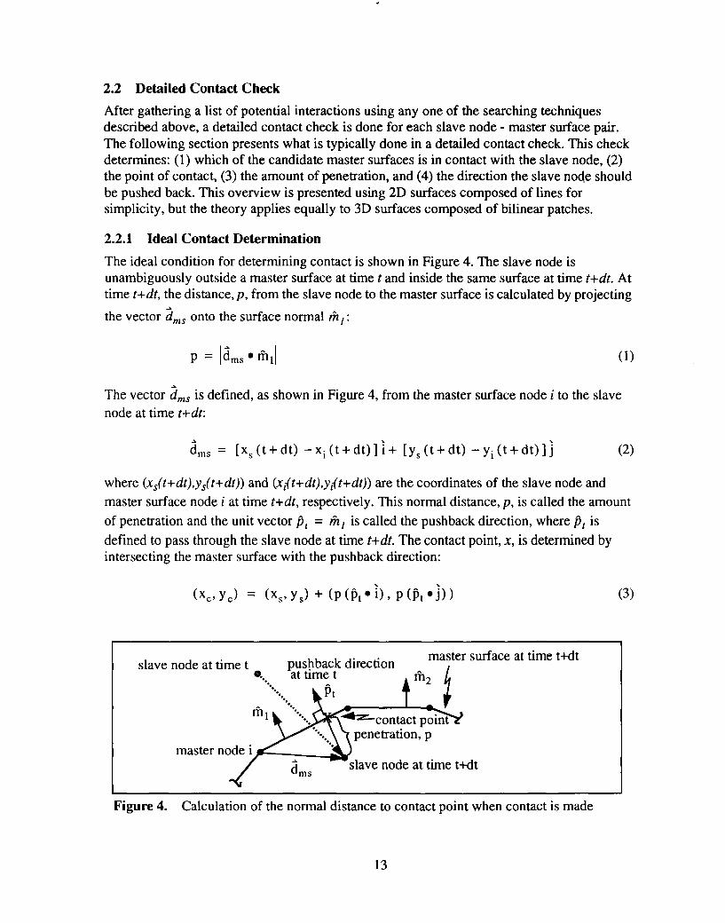
After gathering a list of potential interactions using any one of the searching techniquesdescribed above, a detailed contact check is done for each slave node - master surface pair.The following section presents what is typically done in a detailed contact check. This checkdetermines: (1) which of the candidate master surfaces is in contact with the slave node, (2)the point of contac$ (3) the amount of penetration, and (4) the direction the slave node shouldbe pushed back. This overview is presented using 2D surfaces composed of lines forsimplicity, but the theory applies equally to 3D surfaces composed of bilinear patches.

2.2.1 Ideal Contact Determination

The ideal condition for determining contact is shown in Figure 4. The slave node isunambiguously outside a master surface at time tand inside the same surface at time t+dt. Attime t+dt, the distance, p, from the slave node to the master surface is calculated by projecting

the vector ~~~ onto the surface normal r?zf:

p= am, .rill (1)

The vector ~~~ is defined, as shown in Figure 4, from the master surface node i to the slave

node at time t+d~

im, = [x, (t+dt) -xi(t+dt)]~+ [y~(t+dt) eyi(t+dt)]~ (2)

where (x~(t+dt),y~(t+dt)) and (xi(t+dt),y~t+dt)) are the coordinates of the slave node and

master surface node i at time t+dt, respectively. This normal distance, p, is called the amount

of penetration and the unit vector @f = h] is called the pushback direction, where ~f is

defined to pass through the slave node at time t+dt. The contact point, x, is determined byintersecting the master surface with the pushback direction:

(xc, yc) = (x,> Y,) + (P(P, J), P(Pt@j)) (3)

slave node at time t ~sthtec~ directionmaster surface at time t+dt

e.....

●.O..O

master node islave node at time t+dt

Figure 4. Calculation of the normal distance to contact point when contact is made

13

2.2.2 Pushback inaccuracies

Unfortunately, there are many ambiguous cases of contact that arise because of thediscretization of the surface. The surface is discretized as a collection of ~ continuous finiteelement sides in 2D (or faces in 3D). ~ continuity in the geometric interpolation results in asurface normal that is not continuous. This can have adverse effects on the accuracy of thecontact enforcement. Consider, for example, the case where a slave node is sliding across thesurface shown in Figure 5. One must keep in mind that the enforcement of the contactconstraint is not exact in one time step and could be enforced over several time steps. It ispossible then, that the slave node be penetrating the master surface at time t+dt (a time step dtafter contact was detected). As the slave node slides from being in contact with master surface1 to being in contact with master surface 2, the pushback direction is changing to coincidewith the normal of master surface 2. This change in the pushback direction artificiallyintroduces added slave node motion along its trajectory. This is a direct result of the inexactenforcement of the contact constraint in one time step. In calculations where friction ismodelled, this velocity can add noise to the solution.

contact point and contact point and

pushback direction at time t pushback direction at time t + dt(calculated based on normal distance)

master surface 1at time t+dt ~

?%% :Fe 2

slave node at time t+dt added slave node velocitydue to change in pushback direction

Figure 5. Calculation of the normal distance to contact point as point slides on surface

2.2.3 Overdetermined Contact

Further ambiguity is introduced when the contact algorithm performs the detailed contactchecks based only on the estimated (deformed) configuration. For example, Figure 6 showstwo different scenarios where a slave node can make contact with two master surfaces. Sincethe slave node motion is not used to determine how contact was made at time t+dt, twocontact constraints can be defined (one with master surface 1 and the other with mastersurface 2). The algorithm, then, must resolve the overdetermined contact and decide whichcontact constraint to enforce. This is commonly done by determining which master surface is

most opposed to the slave node surface normal [1] [7] [9]. The surface normal fi at a slave nodeis defined as the average of the normals of all the element faces connected to the slave node. A

master surface is most opposed to the slave surface normal when the quantity Iii . fil islargest. It is common to assume that the most opposed master surface is the one on which the

14

contact constraint should be enforced, so that in Figure 6a, the slave node is contacting mastersurface 1 and in Figure 6b the slave node is contac-ting master surface 2. The most opposedcriterion is often called the strength of contact check.

contact point

fill

master surface at time t+dt slave node at time t+dt

ii

(a) slave node more opposed to master surface 1: 16 ● iill > Ifi ● fi121

contact point

rillmaster surface at time t+dt

slave node at time t+dt

(b) slave node more opposed to master surface 2: Iii ● rn21 > Ifi ● fill

Figure 6. Resolving overdetermined contact by determining most opposed master surface.

When two surfaces are already in contact the strength of contact check can be effective.However, when the surfaces are just coming into contac~ as shown in Figure 7, this type ofstatic contact check cannot consistently resolve the overdetermined contact and predict thecorrect contact constraint. In Figure 7a, the slave node makes contact with master surface 1. InFigure 7b, the slave node makes contact with master surface 2. The contacts area result of themotion of the slave node and are not determined by the master surface which is most opposed.

15

slave node at time t

!

master surface at time t+dte----

-...-...fill


(a) contact point on master surface 1

contact point e slave node at time t

iiilmaster surface at time t+dt


(b) contact point on master surface 2

Figure 7. Determining contact point with consideration of slave node’s movement.

2.2.4 Undetermined Contact

Another ambiguity exists when the normal distance is undetermined. Figure 8 illustrates asituation when this can occur. The normal distance measured from the slave node to themaster surface does not intersect any master segment. Intersection implies that the contactpoint, x, on the master surface lies between the ‘master surface nodes, and not beyond them asshown in Figure 8a and b. Current algorithms typically allow an extension, e, of the mastersurface so that contact can be detected. This extension means that either one contact is foundor, in other cases, both contacts are detected and a choice between the two must be made.With either case, the contact point is still incorrectly defiied. This inaccurate determination ofthe contact point causes “contact chatter”, (see example 5.2).

In this situation, the detailed contact check should identify the vertex of the two mastersurfaces as the contact point since it is the closest point on the master surface, as shown inFigure 8c.

16

J?J2(e

...


lilz

+

t

...-..


(a) contact with master surface 1 (b) contact with master surface 2

contact pointslave node at time t

e.+ fill●....

master surface at time t+dt..O

..


(c) contact at vertex of master surface 1 and master surface 2

Figure 8. Resolving undetermined contact by identifying the closet point to the mastersurface

2.3 Motivation for Current Work

Several algorithms for efficient neighborhood identification have been summarized in thissection. These included surface side-set pairing, surface tracking, bucket searching, andpinball contact. This current technology works successfully for a large variety of contactproblems. There are some problems, however, where improvements in neighborhoodidentification and searching are required. Improvements would be beneficial in problemsinvolving: structures that buckle and fold onto themselves; structures that have materials thattear and create new surfaces; multiple body contact/impact; and structures that slide relativelylarge distances over other surfaces.

In particular, improvements could address two distinct concerns with current searchtechniques. One concern is that nearly all neighborhood identification techniques are fornodes. For example, the result of a search is always the closest master node for a given slavenode (with one exception in pinball overlap). A slave node does not always contact a mastersurface connected to the closest master node. Figure 9 shows a very simple shell self-contact

17

example demonstrating this fact. The slave node 2 is tracking master node 14, however it isactually contacting master surface 8-9 (defined by surface nodes 8-9). The tracked masternode 14 implies that a detailed contact check would consider master surfaces 13-14 and 14-15only and not master surface 8-9 as it should. Contact is always made between a slave node anda master su~ace, and an improved neighborhood identification should reflect this.

slave node

contacted master surface 8-9

tracked mastersurface node

Figure 9. Slave node 2 tracking closest master node 14 results in a missed contact

Another concern is that current global sorting and searching routines depend on the problemdomain. The efficiency of bucket searching is adversely affected by problems that grow orexpand in spatial dimension. Significant improvements in the speed and efficiency of thesearch phase could be made if it depended only on the number of master surfaces and slavenodes in the problem, and not on the problem geometry.

The detailed contact check was also summarized in this section. The difficulties associatedwith detailed contact determination included (1) inaccurate pushback direction, (2)overdetermined (multiply defined) potential contact, and (3) undetermined contact. Animproved contact detection algorithm should address these issues and offer improvedaccuracy in determining the contact point, penetration, and pushback direction.

18

3 New Contact Detection Algorithm

The proposed contact detection algorithm outlined in the following section offersimprovements in the efficiency and accuracy of contact detection. The improvements are theresult of a neighborhood identification strategy that uses a global contact search and anaccurate detailed contact check that uses the projected motion of both master and slavesurfaces. The algorithm does not require contact surface pairing and, therefore, easily handlesself-contacting surfaces, eroding and tearing surfaces, and random contact between multiplebodies. The algorithm also resolves the ambiguities that arise because of the surfacediscretization and from using only the deformed configuration for detailed contact checks.

3.1 New Neighborhood Identification Strategy

The proposed neighborhood identification strategy uses a global search to determine whatslave nodes are in close proximity to a master surface. It accumulates these potentialinteractions by constructing a local neighborhood around a master surface and globallysearching for all slave nodes that are in the neighborhood. Two global search algorithms arepresented, one that takes advantage of the characteristics of vector processors, and one thattakes advantage of the characteristics of parallel processing. The efficiencies of each searchalgorithm are still under investigation. Both algorithms have been implemented on computerswith scalar and vector processors. The algorithm for vector architecture uses a new searchroutine developed by Swegle [19]. The algorithm for parallel architecture is an extension ofthe state-of-the-art bucket searching technique [12], with a few significant exceptions.

To illustrate the two search algorithms, the example shown in Figure 10 of two blockscontacting each other will be used. Each block is a cube with dimensions l“X 1“x l“. Thecentroid of block 1 is initially at the coordinates (0.5”, 0.5”, 0.5”) and is moving with avelocity VY= 500 irds in the y-direction. The stable time step is approximate y 1.1x 10-6s sothat block 1 moves approximately 5.5x104 inches during one time step. Block 2 is initially atrest with its centroid located at the coordinates (0.5”, 1.5”, 0.5”). The symmetric contactenforcement being used implies that every node and element face on the surface is included inthe contact surface. There are 52 slave nodes (rz=52) and 48 master surfaces (m#8).

3.1.1 Algorithm for vector architecture

A search algorithm using 7n memory locations and requiring on the order of mJog2ncomparisons is utilized for the global location strategy. The algorithm is based on a particlesearch technique developed by Swegle [19]. It sorts the slave nodes by location and uses abinary search to construct a list of slave nodes that are in a master surface neighborhood. Thesearch algorithm implemented here depends only on the number of slave nodes n and not onthe geometry of the problem. It takes advantage of the known positions of the slave nodes andmaster surfaces as well as their predicted positions in the next time step.

The slave nodes are sorted based on their current coordinates, with each coordinate sortedindependently. This sorting is done using an index vector so that the order of the slave nodeslisted in the index vector corresponds to their coordinate value, with coordinates ordered fromsmallest to largest. For the current example, there are 52 slave nodes numbered as shown inFigure 10, resulting in the following index vectors:

19

initial velocity of block 2

ij =

block 2

/ ‘

, ( ‘ block 1

/ ‘

x

{0,0,0}

master surface 5

initial velocity of block 1

GI = {O, 500 in/s, O}

44

36 3’/ 435

27 28

Figure 10. Example of two blocks contacting each other.

lx= { 1,4,7,10,13,15,1 8,21,24,27,30,33,36,39,4 l,U,47,5O,2,5,8,l 1,16,19,22,25,28,31,34,37,42,45,48,5 1,3,6,9,12, 14,17,20,23,26,29,32,35,38,40,43,46,49,52 )

IY= { 1,2,3,4,5,6>7,8,9,10,1 1,12,13,14,15,16,17,18,19,20,21,22,23,24,25,26,27,28,29,30,3 1,32,33,34,35,36,37,38,39,40,41 ,42,43,44,45,46,47,48,49,50,51,52 }

Iz = { 7,8,9,15, 16,17,24,25,26,33,34,35,41,42,43,50,5 1,52,4,5,6,13,14,21,22,23,30,31,32,39,40,47,48,49,1,2,3,10,1 1,12,18,19,20,27,28,29,36,37,38,44,45,46 }

for the x, y, and z coordinates respectively. A rank vector is also constructed for the slavenodes. It gives the location of each slave node in the index vector and is required to avoidsearching the index vector for a given slave node. It can be easily constructed by loopingthrough the index vector. For example, suppose a slave node i is stored at position j in theindex vector. The rank vector would then store the pointerj at its position i. For the currentexample, the rank vectors are:

20

RX={

RY=(

Rz={

1,19,35,2,20,36,3,2 1,37,4,22,38,5,39,6,23,40,7,24,41 ,8,25,42,9,26,43,10,27,44,11,28,45,12,29,46, 13,30,47,14,48,15,31,49, 16,32,50,17,33,51,18,34,52 )

1,2,3,4,5678910,1 1,12,13,14,15,16,17,18,19,20,21,22,23,24,25,26,77>??27,28,29,30,3 l,32,33,34,35,36,37,38,39,@,4l,42,43,U,45,46,47,48,49,50,51,52 }

35,36,37,19,20,21, 1,2,3,38,39,40,22,23456 41 ,42,43,24,25,26,7,8,9,?9?744,45,46,27,28,29,10,1 1,12,47,48,49,30,31,13, 14,15,50,51,52,32,33,34,16,17,18 }

After the slave nodes are sorted by x, y and z coordinate, the master surfaces are processedsequentially. This processing involves defining a local neighborhood for each master surfaceby bounding the space occupied by a master surface at its known location at time tand itspredicted location at time t+dt.Figure 11 shows a bounding box for a master surface over onetime step. Another box, called the capture box is also constructed to collect slave nodes thatpotentially contact the master surface.

current position predicted position\< , ~ (vz)tnaxdt

bounding box \

capture box ~\ @

63

69

t 75slave

@ ““”“~i$&M:.:.::M..........................~...:.’.,:.:.::~

node @ @ ““;’w&””

@@ (vY)rnmdt-“dt

@

Figure 11. Bounding box and capture box for a moving master surface

For example, suppose the maximum distance any slave node moves in one time step is(vx)mmdt in the x-direction. Then a slave node within a distance (vx)mmdt from the bounding

box could potentially contact the master surface. This holds for the y- and z-directions as wellso that a capture box can be constructed, as shown in Figure 11. Any slave node inside thecapture box should therefore be considered for potential contact with the master surface. In

the example problem, (Vx)mm = O, (Vy)m= = SOO i~$ (Vz)m= =0, and dt= 1.1x10-6 s,sothe

capture box for master surface 5 would have the corners:

21

X~ln = 0.0 in., xmax = 0.5 in.

Y~l” = 1.0 – vYdt = 0.99945 in.

Z~ in = 0.5 in. , z~,x = 1.0 in.

, Yin,, = 1.0+ vYdt = 1.00055 in,

At this point it is necessary to address one aspect of the contact enforcement algorithm thatwill affect contact detection. Recalling that a contact constraint is likely to be enforced overseveral time steps, the capture box must be enlarged to capture slave nodes with a partiallyenforced contact constraint. A distance, pr, equivalent to the amount of penetration notenforced is easily computed for each slave node in contact with a master surface, as shown inFigure 12. The capture box is enlarged in all directions by this distance, pr.

Icontact oint and

\remaining penetration

pushbac direction at time t , at time t+dt

master surface 1at time t+dt

master surface 2penetration at time t at time t+dt

slave node at time tenforced position ofslave node at time t+dt

Figure 12. Remaining penetration due to a partially enforced contact constraint

After defining the capture box a binary search is done on the index vectors to find the slavenodes that are inside the capture box. The binary search results in hvo pointers for eachcoordinate direction. One is a lower pointer into the index vector that corresponds to theposition in the index vector of the first slave node inside the capture box and the other is anupper pointer that corresponds to the position in the index vector of the last slave node insidethe capture box.

For the example problem node 1 at position 1 in Ix is the frost node in the box in the xdirection, and node 51 at position 34 in Ix is the last node inside the capture box. In theydirection node 18 in position 18 of IYand node 35 at position 35 in IYare the frost and lastnodes just inside the capture box, respectively. Similarly, in the z direction node 4 in position19 of Iz and node 46 at position 52 in Iz are the f~st and last nodes inside the capture box,respectively. Therefore, the binary search would give the following results:

(ix)min = 1, (ix)mn = 34

(iy)min = 18, (iy)m= = 35

22

(iz)rnin = 19, (i&m= 52

This means, for example, that the subset of slave nodes from Ix((ix)min) to Ix((ix)mm) are inthe capture box of the master surface on the basis of the x-coordinate. For the exampleproblem, the subset or list of slave nodes for each coordinate direction that are in the capturebox of master surface 5 are:

LX= { 1,4,7,10,13,15,1 8,21,24,27,30,33,36,39,4 l,M,47,5O,2,5,8,l 1,16,19,22,

q={

Lz={

25,28,31,34,37,42,45,48,5 1 }

18,19,20,21,22,23,24,25,26,27,28,29,30,3 1,32,33,34,35 }

4,5,6,13,14,21,22,23,30,3 1,32,39,40,47,48,49, 1,2,3,10,11,12,18,19,20,27,28,29,36,37,38,44,45,46 }

Finally, a contraction is done to find the slave nodes in the capture box of the master surface inall three coordinate directions simultaneously. To accomplish this, each of the slave nodes inone list is selected and then checked if its rank is between the lower and upper pointer in theother two coordinates. For computational efficiency the shortest list of slave nodes is selected,which can be determined by selecting the smallest of [(iW)mm - (iW)m~ + 1] , w = x, y, or z.

For the example problem, ~ is the list with the smallest number of slave nodes, so that slave

nodes i = IY( (iY) ~in), IY( (iY) ~in + 1), ... . IY( (iY) ~aX) are in the capture box if

‘ix) ~i~ S ‘X ‘i) < ‘ix) ~~~ and (iZ) ~in < Rz (i) S (iz) ~,x.

To help illustrate this procedure, the frost few slave nodes in list ~ are processed as follows:

1) i = IY((iY)~in) = 18 ,Rx(18) =7, and Rz(18) =41.

Since (iX)~in S7 s (iX)m,X and (iz)~in s41 < (iz)~,, slave node 18 is in

the capture box of master surface 5.

2) i = $( (iY)~in+ 1) = 19, Rx(19)= 24, and RZ(19) =42.

Since (iX) ~in <24 S (i,) ~,, and (iZ) ~in <42 S (iZ) ~,X slave node 19 is also

in the capture box of master surface 5.

3) i = IY( (iY)~in +2) = 20, RX(20) = 41, and RZ(20) = 43.

Since 41> (i,) ~,, slave node 20 is NOT in the capture box of master surface 5.

After processing all of the slave nodes in list Ly, it is found that only the slave nodes{18,19,21,22,27,28,30,31) are within the bounding box of master surface 5.

For efficiency on a vector computer each slave node-master surface pair is stored in an array

23

for later processing after a vector length of pairs is accumulated. Note that only those pairs areadded where the slave node is not also a node on the master surface. For the example problemonly the following four pairs would be added to the array:

{ (27, 5), (28, 5), (30,5) and (31,5) }

At this point an exhaustive search has been done and no assumptions have been made on themanner in which contact can or will be made. The processing that will determine contact iscalled the detailed contact check. In the current implementation of the algorithm, the binarysorting is implemented every time step.

3.1.2 Algorithm for parallel architecture

The following algorithm is essentially a conventional bucket search [12] with two significantexceptions. These exceptions are that (1) the bucket size b~ is based on the smallest mastersurface dimension and (2) a capture box is used to ensure all potential contacts are gatheredfor a detailed contact check. The capture box takes advantage of the known positions of theslave nodes and master surfaces as well as the predicted positions in the next time step. Bothare described in detailed after the bucket search algorithm is reviewed.

The bucket search algorithm f~st sorts the slave nodes into buckets, then finds the buckets thata master surface occupies and pairs the master surface with the slave nodes in those buckets. Itrequires (18n) memory locations plus two vectors with lengths equal to the number ofbuckets (rib).

To sort the slave nodes into buckets, an integer coordinate system is constructed in eachphysical direction. Assuming that the bucket size b~ is based on the dimension of the smallestmaster surface, the number of slices (each with thickness bs) required in the x, y, and zdirections are:

s= = int[ (Xm~~–Xml~ ) /b~] + 1

Sy = int [ (Ymax– Ymin)lb,] + 1

Sz = int [ (z~~x–z~i~) /b,] + 1

The three slices containing any given node, i, can be calculated as follows:

S; = int [ (xi – Xmin) /b~] + 1

S; = int[ (yi_ymin) /b,] + 1

S: = int [ (zi_zmin) /b~] + 1

The intersection of the three orthogonal slices defines the bucket Bi containing node i, asshown in Figure 14.

24

(Xmim Ymax>%nin)

.F(xmin~Ymirp‘ma.x)

@lV s;

Figure 13. Bucket Bi defined by three slices of the data that contain node i.

If buckets are numbered sequentially, progressing fiist in the x direction, next in the ydirection, and then in the z direction, the bucket id containing node i is given by;

Bi = (B~-l)SXSY +( Bj-l)SX+B~

With the eventual aim of efficiently determining a list of slave nodes within any given bucke~two vectors of length n are created. One stores the bucket id for each slave node, fbox, and theother is a list of slave nodes sorted by bucket id, nukort. Two additional vectors of length nbare also constructed to efficiently access the slave nodes. The f~st contains the number ofslave nodes occurring in each bucket, nbox, and the other is a pointer that identifies the firstslave node in each bucket, npoint. The entire sorting procedure can be summarized as follows:

1.

2.

3.

4.

5.

6.

Zero the vector (nbox) containing the number of nodes in each bucket.

Find the bucket id (Bi) for each node.

Store the bucket id for node i in the vector: fbox(i) = Bi

Increment the counter for bucket Bi: nbox(Bi) = nbox(Bi) + 1

Calculate the pointer for each bucketj into a sorted list of nodes.

npoint(l) = 1 npoint(j) = npointfj-1) + nbox(j-1)

Zero the vector nbox

25

7. Sort the slave nodes according to their bucket number into a list nakort.

nakort(nbox([box(i)) + npoint(lbox(i))) = i

nbox(lbox(i)) = nbox(lbox(i)) + 1

For the example problem, the bucket size is 0.5 inches corresponding to the dimension of thesmallest master surface. This implies that Sx =3, SY= 5, and Sz = 3 and a total number ofbuckets nb = 45. The bucket sort of all 52 slave nodes would give the following results:

Bucket id for each slave node:

lbox = {3 1,32,33,16,17,18,1,2,3,34,35,36, 19,21 ,4,5,6,37,38,39,22,23,24,7,8,9,

Pointer into ndsort

37,38,39,22,23,24,7,8,9,40,41 ,42,25,27,10,1 1,12,43,44,45,28,29,30,13,14,15)

giving the starting location of the slave nodes in each bucket:

npoint = {1,2,3,4,5,6,7,9,11,13,14,15,16, 17,18,19,20,2 1,22,23,23,24,26,28,30,3 1,3l,32,33,34,35,36,37,38,39,4O,4l,43,45,47,48,49,5O,5 1,52}

List of slave nodes sorted by their bucket id:

ndsort = (7,8,9, 15,16, 17,24,33,25,34,26,35,41 ,42,43,50,51,52,4,5,6, 13,14,21,30,22,3 1,23,32,39,40,47,48,49 12310,1 1,12,18,27,19,28,20,29,36,37,979?38,44,45,46}

Number of slave nodes in each bucket:

nbox={l,l,l,l,l,l,2,2,2,1,1,1,1,1,1,1,1,1 1012221011111111112229?77937>>9 >> 77799977 >>1,1,1,1,1,1}

To illustrate how all slave nodes within, for example, bucket 23 are gathered, the sortedinformation described above is used as follows. The number of slave nodes in bucket 23 isgiven by: nbox(23) = 2. The slave nodes occupying bucket 23 can be found starting at locationnpoint(23)=26 in ndsort. This implies that slave nodes at location 26 and 27 in ndsort are inbucket 23: ndsort(26-27) = slave nodes {22,31).

The sorting algorithm above is identical to that described in [ 12][ 16]. Potential interactionsbetween nodes in [12] [16] are determined by looping through the buckets and collecting theslave nodes in neighboring buckets, using the pointer into the sorted list. This implies that thebucket size must be based on the largest master surface dimension to avoid missing potentialcontact, as was demonstrated in Figure 3.

To avoid these difllculties, the strategy that the proposed search algorithm employs is tocollect all the buckets occupied by a master surface. Then, using the information obtainedduring sorting, the slave nodes in those buckets are collected. This ensures that all potential

26

interactions with a given master surface are found regardless of bucket size (and thereforeproblem geometry). Lnthe current algorithm, the bucket size should be interpreted as thesorting refinement instead of a length measure of the largest master surface. A bucket sizebased on the smallest master surface assures that there will be a small number of slave nodesin each bucket and admits the possibility that a master surface could occupy many buckets.

The collection of slave nodes with which a master surface could potentially interact isdetermined in the following way:

1. A capture box is constructed for each master surface, as described previously

2. The buckets containing the extreme comers of the master surface capture box aredetermined

iboxmin = min( SX, iflx( (xcmin-xmin)b, )+l)

jboxmin = min( SY, ifix( (ycm~-ymin)b~ ) + 1 )

kboxmin = min( Sz , ifix( (ZC~in-Zmin)/bS ) + 1 )

iboxm~ = min( Sx , ifix( (xcmm-xmin)/bs ) + 1 )

jboxmm = min( SY, ifix( (ycmm-ymin)/bs ) + 1 )

kboxm,m = min( SZ , ifix( (ZCmax-’Zmin)/bS ) + 1 )

where xcmin and xcmcware the comers of the master surface capture box in the xdirection (ycmin, ycmax, zcm~ and zcmm have the same definitions in the y and zdirections, respectively).

3. All buckets within the ranges calculated in step 2 are identified as follows:

Loop from ibox = iboxmin to iboxmm

LOOP from jbox = jboxmin to jboxmm

Loop from kbox = kboxlnin to kboxmm

B*= (kbox-l)SXSY + (jbox-l)SX + ibex

Endloop

Endloop

Endloop

4. All slave nodes in the buckets calculated in step 3 are considered for potentialinteraction with the master surface

In this approach, the algorithm takes advantage of the observation that the buckets that amaster surface occupies can be easily determined. Lnthe example problem, assume thatmaster surface 5 is to be processed. The comers of the capture box of master surface 5 are:

27

XC~in= 0.0 ill., XC~~= 0.5 iI1.

ycm~ = 0.99945 in., ycmn= 1.00055 in.

zcm~ = 0.5 in., zcmm= 1.0 in.

so that the capture box would occupy the range of buckets:

iboxmin = 1 , iboxmm = 2

jboxmin = 3, jboxmn = 3

kboxmin = 2, kboxmm = 3

This identifies buckets 22,23,37, and 38. The slave nodes occupying these buckets would beconsidered for potential contact with master surface 5. Note that only the slave nodes whichare not also nodes on master surface 5 are considered, so that only the following four pairswould be added to the vectonzed list:

{ (27, 5), (28, 5), (30,5) and (31,5) }

In the current implementation of the algorithm, the bucket sorting is implemented every timestep in a vectorized mode. A study of the efficiencies of a bucket search algorithm waspresented by Plimpton [20] for a computer with parallel architecture. For a certain class ofspatially compact problems, the bucket searching seems to be faster than the vectorized globalsearch. Further speed up might be anticipated by sorting every 5 to 10 time steps, suggested by[12], while storing the nearest neighbors for contact determination in the intermediate timesteps.

28

3.2 New Detailed Contact Check

The proposed detailed contact check distinguishes between slave nodes that are not in contactand those that are already in contact. It does so to resolve the ambiguities that arise in eachcase. The ambiguity shown in Figure 7, for example, could be easily resolved by consideringthe velocity of the slave node. This idea of a velocity based contact check can be extended toinclude a moving slave node contacting a moving master surface, as shown in Figure. 14a. Forslave nodes just coming into contact the velocity based contact check identifies the point ofcontact (or impact) and the contact time. Figure 14b shows a static contact check that is usedfor slave nodes already in contact with a master surface. For these slave nodes, ambiguitiesarise because the surface normal is not continuous. This can result in not finding any contactwhen there should be one or finding multiple solutions to a single contact. The proposedvelocity based and static based detailed contact checks resolve these ambiguities, as shown inthe following sections.

slave node

slaye noat time t+

master surfdceat time t

solve for:

● time untilcontact occurs (dt)

● coordinates of

contact point (x)

(a) velocity based contact check based on position and velocity

@

\\ . ...”’----

solve for:

\● coordinates of the nearest

ipoint to surface (x)

slave node master surfaceat time t+dt at time t+dt

(b) static based contact check based on position

Figure 14. Master slave tracking using velocity and static contact check

3.2.1 Velocity Based Contact Check

The velocity based contact check makes use of the current position of the surfaces and theestimated velocities in the following time step. The contact check is restricted to a movingtriangular master surface and a moving slave node for 3D, as shown in Figure 14a.

29

The hi-linear quadrilateral master surface is subdivided into four triangular master surfaces.The four triangles are defined by the four comer nodes of the quadrilateral plus an added fifthnode located at its centroid. In 2D, the master surface is a moving line, and is just a specialcase of the 3D moving contact presented below. A complete derivation of the velocity basedcontact check can be found in Appendix 1.

The equation of a triangular master surface (a plane) can be written as:

a(x–xl) +b(y–yl)+c(z–zl) =0 (4)

The point (xl, y,, Zl) is a node on the master surface, and a, b, and c are components of the

master surface normal ~m = a; + b~ + c~, where:

a= [(yl–y3) (zz –21) – (Y2– Y1) (21–23)1

b= [(x2–xI) (Z1–z~) – (xl–x3) (22–21)1

c= [(X1–X3) (yz–y~) – (X2–X1) (Y1– Y3)I

(5)

Here, x2, y2, Zzand X3,yq, z~ are coordinates of the other nodes defining the triangular mastersurface. Now, note that the triangular surface is moving, so that:

[( xi(t+At) >yi(t+At) >zi(t+ At)) =

(xi (t) +xiAt> yi (t) +jiAt> zi (t) + ziAt) ], i = 1>3(6)

and the slave node is also moving, so that:

( x,(t+At), y,(t+At), z,(t+ At)) =

(X, (t) + x,At, y, (t) + y~At, 2, (t) + z,At)(7)

Following these definitions, a time At is sought such that the slave node will be co-planarwith the three nodes defining the triangular master surface. Such a time can be found (if itexists) by substituting equations (5), (6), and (7) into equation (4) and solving a cubicequation in At (see Appendix 1).

Suppose a solution At = AtC is found. Then it also must satisfy two conditions for it to be

considered a contact. The first is that the time Atc occurs in the next time step increment,

O < AtC < dt. The other condition is that the contact point:

(xc,Yc> Zc) = (x, + x,Atc> Y,+ y,Atc> z,+ Z,At.) (8)

30

must lie inside the edges of the quadrilateral master surface. This can be determined exactly

by computing the local ~, q coordinates of the contact point on the quadrilateral master

surface. Figure 15 shows how an initial estimate go, q ~ of the local coordinates can be

computed. Four triangles are constructed by connecting the contact point with the four cornersof the quadrilateral master surface. The contact point is inside the master surface when all fourareas A 1, A2, A3, and A4 are greater than or equal to zero and Al + A3 >0 and A2 + A4 z O. If

this condition is met, then an initial estimate of the local coordinates of the contact point canbe found, as shown by the equations in Figure 15.

initial estimate ofcontact point

0

!()=2A~A-124

Al~0=2A1+A~–*

Figure 15. Initial estimates for the local coordinates of a contact point

The logic for these equations is based simply on the observation that (~, ~) = (5., ~o) is

computed exactly for any rectangular quadrilateral and that the limiting values of

~ and q = *1 are computed exactly for any shaped quadrilateral. If the quadrilateral surface

is a rectangle, then the proof is simple. If it is not, then by observation ~ is computed exactly

only when one of the areas A2 or A4 is zero. Likewise q is computed exactly only when one

of the areas A 1 or A3 is zero. For example, suppose A2 is zero then the estimated coordinate

~ = go = 1 is exact. If A4 is zero then the estimated coordinate ~ = go = -1 is also exact.

If neither A2 or A4 are zero, then the equation gives a reasonable estimate of the contact point

~. Improvements in the accuracy of the local coordinates can be achieved byperfOrm@

Newton iterations on the nonlinear equations relating ~, q, and ~ to ~, yc, and ZC(see

Appendix 1).

In certain cases there maybe multiple master surfaces where contact is possible. The exampleproblem shown in Figure 10 illustrates such a case in which a slave node contacts multiplemaster surfaces. For example, the slave node 27 could contact any one of the three mastersurfaces connected to node 18. In these cases, a strength of contact check is used to determine

the most opposed master surface where ~~ ● (VS – ~~) is minimized. In the example

problem, master surface 5 is the most opposed master surface.

31

3.2.2 Static Contact Check

The static contact check is used for those slave nodes already in contact with a master surface.The contact check is also restricted to a slave node contacting a triangular master surface. Thecalculations are based on the predicted configuration of the surface if the contact forces wereremoved from the surface nodes. This predicted configuration would obviously have slavenodes penetrating master surface elements. In order to bring these interpenetrating surfacesback into compliance, the slave node must be pushed back to the master surface. Indetermining the push back direction, a distinction is made between concave and convexsurfaces.

The push back direction for a concave surface is determined simply by the minimum distanceto the master surface as shown in Figure 16. The push back direction @t+~t can be along themaster surface normal as shown in Figure 16a or it may be defined by the minimum distanceto a vertex as shown in Figure 16b. This choice in pushback direction is done simply to detectan undetermined contact.

fh2

contact point

\r’ill

/slave nodeat time t+dt

master surfaceit tune t+dt

:a) closest point is on master surface 2

contact point

Ihl

t\

‘/master surface bat time t+dt slaye node

at time t+dt

Figure 16. Push back direction for a concave surface

(b) closest Domt IS on vertex ofmaster surface 1 and 2

based on minimum distance to

master surface.

For a convex surface, the push back direction ~t + d~is always along the normal of the master

surface that the slave node was previously in contact with, i.e fhP in Figure 17. In Figure 17a

the slave node was previously in contact with master surface 1 (fiP = fil ) so the pushback

direction is fit+ d~ = rnP = fi ~. Again, in Figure 17b the slave node was originally in contact

with master surface 1 so ~t + d~ = fiP = h 1. After the slave node is pushed back to master

surface 2, the pushback direction is updated to reflect that ~t + .2d~= rn2. This avoids adding

artificial slave node velocity due to a change in pushback direction, as illustrated in Figure 5.

32

fjt = &p contact point

A‘P

= fil

naster surfacet time t+dt

slave nodeat time t+dt

@t = ‘p contact pointA‘P = fil

master surfaceat time t+dt /

slave nodeat time t+dt

(a) closest point is on previousmaster surface

(b) closest point is neighboringmaster surface

Figure 17. Push back direction for convex surface based on previous master surfacenormal.

The contact point, X, on a convex surface is found by the intersection of the triangular mastersurface plane, Equation (4), and a line defined by the parametric equations:

x=x~+s(fipoi)

Y= Ys+s(rnp”l)

z=z~+s(lilp. i)

Providing that the master surface and the line are not parallel, the parameters can be found as:

(9)

a(xl–x~) +b(yl–y~)+c(zl –z~). . . (lo)

a(fipoi) +b(fip. j)+c(fipo k)

Just as in the case of a velocity based contact check, there may be some instances wherecontact with multiple master surfaces is possible according to the static contact check. Again a

strength of contact check is used to determine the master surface where fi~ ● ~~ is

minimized.

3.3 Summary of Proposed Contact Detection Algorithm

The proposed contact detection algorithm outlined in this section offers some advantages overthe currently used algorithm in the Sandia codes. It does so by separately considering a fast,memory efficient, global search for potential contacts, and a much more accurate detailedcontact check:

33

● The efficient global search allows for global contact. This means that added capabilityfor modelling self contacting structures and eroding or tearing surfaces is nowavailable. Another benefit of the efficient global contact search is that fewer slavenode - master surface pairs are found as potential contacts. This is possible by takingadvantage of both the known location of the contacting surfaces and their velocities inconstructing a master surface capture box. The capture box ensures that a minimumnumber of slave nodes are paired with the master surface.

● The detailed contact check is more accurate in determining the point of contact,amount of penetration, and the direction of pushback. This results in a physicallycorrect determination of contact constraints. The improved accuracy has also reducedthe number of iterations required for convergence in the iterative solvers in the Sandiaquasistatic codes.

34

4 Surface Definition Algorithm

The proposed contact detection algorithm described in the previous section discussed thedetails of the neighborhood identification and global search, and the detailed contact check.Implied in the discussion was the definition of the entities involved in contact, namely theslave nodes and the master surfaces. Typically this is done using preprocessors such asFASTQ [21], GJOIN [22], GEN3D [23], and GENSHELL [24] to define meshes and sidesets. Side sets are a collection of element faces and their corresponding nodal points. Thecontact algorithm would then require as input the listing of these side sets (without requiringside set pairing). In many applications, such as self contact, this kind of input is all that isrequired. For other applications such as tearing or eroding surfaces, the contact surface ischanging during the execution of the problem. In these types of problems, a dynamicallydefined surface (composed of all master surfaces and slave nodes on the surface) is essential.

For this purpose, an algorithm for automatically determining the surface of an arbitrary meshcomposed of hexahedral and shell elements is proposed. The surface definition algorithm usesa data structure that allows the initial surface definition and an incrementally updated surfacewhen necessary. In the algorithm, shell elements are considered as a subset of hexahedralelements. For clarity, the following discussion is limited to a mesh composed of hexahedralelements. The algorithm requires 6 x ne memory locations for a mesh composed of ne 8-nodehexahedral elements and involves two simple steps. The first step is to construct a face id forevery element face:

faceid = ndia~ + nmin X nnod (11)

where nnod is the total number of nodes in the problem, nm”nis the smallest global nodenumber defining the element face, and ndiugis the global node number that is diagonal to thesmallest global node nmin. Step two is to search for all face id’s for any non-repeated numberswhich will correspond to the faces that are on the surface. The search is efficiently done usingthe CRAY UNICOS library routine wheneq [25]. Figure 18 shows an example of a 3D meshcomposed of two hexahedral elements.

element 1

Figure 18. Example mesh for surface definition algorithm

35

Table 1 lists the 12 element faces in the mesh, their connectivity, nm”n,ndiag, and their face id.In the example problem, all element faces are on the surface except element 1- face 6 andelement 2- face 5 (which have a the same face id of 67).

II Table 1. Surface definition algorithm example

element face map

number number connectivityy nm.n ndkg (faceid)(iele) (iface)

1 1 1562 1 6 18

1 I 2673 1217131

1 3 3784 3 8 44

1 4 4851 1 8 20

1 5 1234 1 3 15

1- 6 5876 5 7 67

2 1 59106 5 10 70

2 12 I 610117 16111]83

2 3 711128 7 12 96

2 4 81295 5 12 72

2 IS I 5678 1517167

2- 1 6 I 9121110 I 9 I 11 I 119

The result of collecting all the element faces with unique face ids is a list of the mastersurfaces. The slave nodes can be determined by looping through the master surface list andflagging the nodal points defined by the master surface connectivity.

The array called smap initially stores the faceid of each face, as shown in Table 1. For everyelement face on the surface (ones with a unique face id), a zero is over-written insmap(6*(iel.e-l) +iface). For those intenor element faces (ones without unique face ids), apointer to the opposing face is stored in the array, snzap:

smap (6 (ielei – 1) + ifacei) = 6 (ielej – 1) + ifacej

smap (6 (ielej – 1) + ifacej) = 6 (ielei – 1) + ifacei

Using this surface map array, the surface can be incrementally updated as elements aredeleted. For the current example there are only two opposing faces, element 1 face 6 andelement 2 face 5, so that smap(6) = 11, smap( 11) = 6, and all other positions in smap would bezero.

This idea of collecting master surfaces and slave nodes into a heap allows modelling ofcontact between a variety of finite element types. For example, the nodal points of elementssuch as beams and trusses can be added to the slave node list. Also, the potential contacts in aproblem coupling the finite element method with other methods can be modelled. Forexample, particle methods such as Smooth Particle Hydrodynamics (SPH) [26] or Particle-In-Cell (PIC) [27] can be easily coupled by adding the particles to the slave node list.

36

5 Example Problems

The examples considered in this section demonstrate both the improvements in the accuracyof contact detection and the added capabilities that are possible with the global searchalgorithm. The improvements in the accuracy of contact detection are demonstrated with anexample of two elastic blocks contacting and an example of contact induced chatter orringing. Some of the added capabilities include modelling (1) structures that buckle and foldonto themselves, (2) structures that have materials which tear and create new surfaces, (3)problems where multiple body contactiimpact is occurring, and (4) problems whereconsiderable sliding between bodies is occurring. (The necessary files for constructing theinput for all example problems are in Appendix 2)

5.1 Contact of Elastic Blocks

The example of two blocks impacting one another is a simple demonstration of the need for anaccurate detailed contact check. The new contact algorithm correctly chooses the mostopposed master surface for each slave node in the two cases shown in Figures 19 and 20. Thetwo different cases are described as follows:

Case 1. The elastic blocks already discussed in the previous sections and shown in Figure 10are impacting at a velocity VY=500 in/s, as shown in Figure 19. Each comer node hasthe potential of contacting three different master surfaces, and each edge node has thepotential of contacting four different master surfaces. The new contact algorithmduplicates the results of the old algorithm by correctly enforcing the most opposedcontacts.

500 injs

impact (t= O) t = 0.5 milliseconds

Figure 19. End-on impact of two blocks

37

Case 2. The same two blocks in Figure 10 are repositioned such that a comer of Block 1 isimpacting a comer of Block 2, as shown in Figure 20. The old static contact check,which is based on surface normals, chooses the incorrect master surface causing bothblocks to rotate clockwise. By incorrectly determining the pushback direction, a largeincrease in kinetic energy (from 92.5 in-lbs to 1300 in-lbs) results. The new contactdetection algorithm correctly determines the initial contact using the velocity basedcheck and the subsequent updated contact using the static based check. This results inthe correct counterclockwise rotation of both blocks.

%

?500 inis

initial position andvelocity of blocks

f.d

& \old contact

PaA

--%/

\\\+

new contactalgorithm

-\. algorithmt = 0.2 milliseconds “\\\ t = 0.2 milliseconds

\\\

\*

.2

Figure 20. Corner impact of two blocks

38

5.2 Contact Chatter under High Normal Loads: PIKWSUreLoading of ‘IWOElasticBodies

One of the difficulties with two curved surfaces contacting each other under high normalloads is the accurate determination of the push back direction. The example shown in Figure21 has a semicircular rod that is pushed into a semicircular cavity. A pressure load is appliedto the flat surface of the rod. All the nodes on each contact surface are initially aligned witheach other, so that as the pressure is ramped up, the slave nodes on the semicircle (convexsurface) must be pushed back to the vertices of the master surfaces on the cavity (concavesurface). The old algorithm incorrectly determines the pushback direction and introducesnoise (contact chatter) into the solution. This eventually accumulates over many time stepsand results in mesh hourglassing and increased kinetic energy, as shown in Figure 22. Thenew contact detection algorithm correctly determines the pushback direction and does notintroduce noise.

time, t

Fixed

Figure 21. Two elastic bodies contacting under high normal load.

39

o.k!-___Jo. 0.7 1.4 2.1

time (milliseconds)

Figure 22.

o. 0.7 1.4 2.1time (milliseconds)

(a) old algorithm (b) new algorithm

Kinetic energy history and deform~ shape (displacements magnified by 100x)using old and new contact detection algorithm

40

5.3 Self-Contacting Impact: Buckling of Shell-Like Structures

The following example demonstrates the self contacting capability of the contact detectionalgorithm. This feature is important for modelling crash dynamics where buckling, tearing,and self contact is common. The elastic-plastic shell-like (can) structure shown in Figure 23 isimpacted by an elastic-plastic plate. The can is 0.25 inches thick, has an inside radius of 5inches, and is 15 inches long. The bottom of the can is constrained in all directions. The22x 11 in. plate is 2.5 inches thick and is initially tilted at a 10 degree angle as it impacts thecan at 5000 in/s.

The contact detection algorithm currently in PRONT03D is a surface tracking algorithm thatrequires surface pairing. The amount of user intervention required to intermittently define andpair many contact surfaces would make this problem impractical to solve using the currentalgorithm. In contrast, the new algorithm requires two surface ids (one for the plate and onefor the can). Contact between any of the slave nodes and master surfaces on both surface setsare detected during the analysis. The deformed shapes at various times are shown in Figure24. The self-contact of the buckled can is evident in several locations.

ocity 5000 in/si

Figure 23. Fh_iiteelement mesh of an elastic plate impacting an elastic-plastic can

41

(b) t = 2.2 ms

(c) t = 3.3 ms (d) half-section at t = 3.3 ms

Figure 24. Deformed meshes of the buckled can at various times

42

5.4 Automatic Contact Surface Redefinition: Cutting of a Steel Pipe

In the following example, the capability of automatically redefining the contact surface isexercised. For this problem, and others like it, the new surface that is generated as a result oftearing can find itself in contact with other surfaces of the body. The current capabilities of theSandia codes do not include a periodic redefinition of the contact surface. The new algorithmautomatically redefines the surface after any elements are deleted.

The algorithm is demonstrated with a simulation of a pipe cutting process. The processinvolves a hardened, 0.25 inch thick, wedged-shape cutting blade that is forced through a twoinch, schedule 40 pipe that is resting on a support, as shown in Figure 25. The blade initiallyindents and punctures through one side of the pipe and then progressively tears the pipe wall-s,as shown in Figure 26. The tear is simulated by deleting elements in which the material dam-age has accumulated to 0.9. The power law hardening material accumulates damage when itexceeds a failure strain of 1.27 and is loaded under hydrostatic tension [28]. The newly cre-ated surface is automatically included in the contact algorithm by redefining the surface afterany elements are deleted. As the simulation progresses, the edges of the tear are in contactwith the moving cutting blade, as shown in Figure 26. The simulation continues until theblade cuts through the pipe at approximately 3 milliseconds.

Specified velocity= 1187.5 inls

Cutting blade

tip

Figure 25. Finite element model for simulating the cutting of a 2 inch steel pipe.

43

WtiY”‘a)””’milliseconds

Figure 26. Pipe cutting simulation results at various times

44

milliseconds

(d) 3.0 milliseconds

Figure 26 (cent’d). Pipe cutting simulationresults at various times

45

5.5 Multi-Body Impact: Elastic-Plastic Bar impacting Bricks

One of the added capabilities of the new contact detection algorithm is the efficient modellingof multi-body impact without a-priori definition of contact surfaces. The example, shown inFigure 27, has an elastic-plastic bar impacting a stack of 17 elastic bricks. A stationary elastic-plastic wall is also resting against the stack of bricks. All slave nodes and master surfaces onthe bodies were automatically defined using the algorithm described in Section 4.

For problems where random contact is anticipated, as in this example, each body couldpotentially impact any other body. For a contact-pairing algorithm, 1~ contact pairs would benecessary, with each pair having 2n slave nodes. For the new global contact searchingalgorithm, one search with 19n slave nodes is necessary. Assuming that each block hasn = 50 slave nodes, 192 pairs would require 192(2nlog(2n)) = 239,843 comparisons, whereas

the new global contact searching algorithm would require only 19nfog2(l 9n) = 9397comparisons.

Another important feature of the contact detection algorithm is the spatial independence of thenlogn vectorized sorting algorithm. The speed and efficiency of the algorithm is nearlyindependent of the location of the bricks. This becomes particularly important late in thisexample since the volume that the bodies occupy is increasing, as shown in Figure 28.

- elastic-dastic rod with I

initial velocity

Figure 27. Elastic-plastic bar impacting a stack of 17 elastic bricks

46

Figure 28. Multi-body impact simulation results at various times

47

5.6 Large Sliding Contact: Elastic-Plastic Forging of a Copper Billet

The following example demonstrates the capability of modelling large sliding contact typicalin large deformation forming and forging. The quasistatic axisymrnetric forging of a copperbillet shown in Figure 29 was simulated with the program SANTOS. The billet has an initialradius of 2 inches and height of 5 inches. Figure 30 shows a series of deformed meshes as thebillet is forged. As the billet is compressed, it slides horizontally until the die cavity is filled.After further compression, the billet is forged around the die comer forming the rivet head.

There are two difficulties related to contact detection in this example. The f~st is the accuratedetermination of the pushback direction of the slave node in the lower comer of the die. It isinitially constrained on the horizontal master surface as the billet is compressed. Then, just asthe billet fills the die cavity, the slave node is constrained on the vertical master surface. Uponfurther loading, gradual adjustments in the pushback direction are automatically made so thatit is constrained to the vertex of the horizontal and vertical master surface. (The currenttracking algorithms do not push the slave node back to the vertex of the two master surfaces.This results in contact chatter similar to that described in example 5.2.)

Another difficulty arises from the large sliding contact of the material in the billet around thedie corner (shown enlarged in Figure 30). The new contact detection algorithm determines theupdated contact point and pushback direction such that the slave nodes on the billet are notgiven any added artificial velocity.

F@me 29. Finite

I elastic die IJ

I

elastic die

rrdie cavity

4

element mesh of a rivet

48

forging :ocess

IJ

t rI I I

r=o

I

I

I

r=2.0”1 u

Figure 30. Rivet forging of a copper billet

r=l.2° r=l.(j”

r=z.()”

49

6 Conclusions

The current contact detection techniques used in the Sandia structural analysis codes havebeen reviewed. The review has pointed out several areas where improvements are necessaryin current contact detection techniques. These areas include neighborhood ident.iflcation anddetailed contact checking. The neighborhood search should not rely on a closest master nodeto a slave node, and it should be independent of the problem geometry. In several cases, thedetailed contact check requires improved accuracy in determining the contact poin~penetration, and the pushback direction.

A new contact detection algorithm has been presented that offers improvements in these areas.The improvements are a result of a neighborhood identification strategy that uses a globalcontact search and a detailed contact check that distinguishes between concave and convexstiaces. The key features of the new contact detection algorithm are:

● The efficient global search allows for global contact. This means that added capabilityfor modelling self contacting structures and eroding or tearing surfaces is nowavailable.

● The known locations of contacting surfaces and their velocities are used to construct amaster surface capture box. This guarantees that only physically meaningful contactsare considered in the detailed contact check. The capture box also ensures that aminimum number of slave nodes are paired with the master surface.

● The position and velocity of both the slave node and master surface are considered indetermining initial contact. This results in a physically correct determination of thecontact location.

● A distinction between a concave and convex surface is made for slave nodes already incontact with a master surface. This results in a more accurate determination of thepoint of contact, amount of penetration, and the direction of pushback.

● An automatic surface definition algorithm allows for a simplified user input in manycases. One can, for example, include all surfaces of a body by specifying that thematerial be considered for global contact.

The capabilities of the new contact detection algorithm have been demonstrated with severalexample problems. Several of the example problems have demonstrated improvements in theaccuracy and efficiency of contact determination. Other problems have demonstrated theadded capability provided by the new alognthm.

50

References7

1

2

3

4

5

6

7

8

9

10

11

Taylor, L.M. and Flanagan, D.P., PRONT02D: A Two-Dimensional Transient SolidDynamics Program, SAND86-0594, Sandia National Laboratories, Albuquerque, NM87185, 1987.

Taylor, L.M. and Flanagan, D. P., PRONT03D: A Three-Dimensional Transient SolidDynamics Program, SAND89- 1912, Sandia National Laboratories, Albuquerque, NM87185.1989.

Attaway, S.W., Update of PRONT02D and PRONT03D Transient Solid DynamicsPrograms, SAND90-O 102, Sandia National Laboratories, Albuquerque, NM 87185,1990.

Stone, C. M., SANTOS: A Two-Dimensional Finite Element Program for theQuasistatic Lurge Deformation, Inelastic Response of Solids, SAND90-0543, SandiaNational Laboratories, Albuquerque, NM 87185, in preparation.

Biffle, J. H., JAC - A Two-Dimensional Finite Element Computer Program for theNonlinear Quasi-Static Response of Soliak with the Conjugate Gradient Method,SAND81 -0998, Sandia National Laboratories, Albuquerque, NM 87185, 1984.

Biffle, J. H., JAC3D - A Three-Dimensional Finite Element Computer Program for theNonlinear Quasi-Static Response of Solids with the Conjugate Gradient Method,SAND87- 1305, Sandia National Laboratories, Albuquerque, NM 87185, inpreparation.

Hallquist, J.O., User’s Manual for DYNA2D: An Explicit Two-DimemionalHydrodynamic Finite Element Code With Interactive Rezoning, Rev. 2, UCID- 18756,Lawrence Livermore National Laboratories, 1984.

Hallquist, J.O. and Benson, D.J., User’s Manual for DYNA3D: Nonlinear DynamicAnalysis of Structures, Rev. 3, UCID- 19592, Lawrence Livermore NationalLaboratories, 1987.

Hibbitt, Karlsson and Sorensen, Lnc., Contact Calculations with ABAQUS - ABAQUSExplicit Users Manual, Hibbitt, Karlsson and Sorensen, Inc., 1992.

Hallquist, J.O., N1KE2D: A Vectorized Implicit, Finite Deformation Finite ElementCode for Analyzing the Static and Dynamic Response of 2-D Solioh With InteractiveRezoning and Graphics, UCID- 19677, Lawrence Livermore National Laboratories,1986.

Hallquist, J.O., NIKE3D: An Implicit, Finite Deformation, Finite Element Code forAnalyzing tk Static and Dynamic Response of Three Dimensional Solids, UCID-18822, Lawrence Livermore National Laboratories, 1984.

51

12

13

14

15

16

17

18

19

20

21

22

23

24

25

Benson, B.J. and Hallquist, J.O., “A Single Surface Contact Algorithm for the Post-Buckling Analysis of Structures, ” Computer Methoa3 in Applied Mechanics andEngineering, Vol. 78, pp. 141-163, 1990.

Chaudhary, A.B. and Bathe, K.J., “A Solution Method for Static and Dynamic Analysisof Three-Dimensional Contact Problems with Friction,” Computers and Structures,Vol. 24, No. 6, pp. 855-873, 1986.

Zhong, Z.H. and Nilsson, L., “A Contact Searching Algorithm for General 3D Contact-Impact Problems,” Computers and Structures, Vol. 34, No. 2, pp. 327-335, 1990.

Harding, D.C., Attaway, S.W., Neilsen, J., Blacker, T. D., and Pierce, J., “Evaluation ofFour Multiple Package Crush Environment to the Common Package, Model 1,Plutonium Air Transport Container,” SAND92-0278, Sandia National Laboratories,Albuquerque, NM 87185, 1992.

Belytschko,T. and Lin, J. I., “A Three-Dimensional Impact-Penetration Algorithm withErosion,” Computers and Structures, Vol. 25, No. 1, pp. 95-104, 1987.

Belytschko,T. and Neal, M. O., “Contact-Impact by the Pinball Algorithm with Penaltyand Lagrangian Methods,” Int. J. Numerical Methods Eng., Vol. 31, pp. 547-572, 1991.

Metzinger, K., Attaway, S., and Mello, F., “Bobbin Stresses Generated by WireWinding,” First International Conference on Web Handling, Oklahoma StateUniversity, Stillwater, OK 74078, May 19-22, 1991.

Swegle, J.W., “Search Algorithm,” Memo to Distribution, Sandia NationalLaboratories, Albuquerque, NM 87185, May 25, 1992.

Plimpton, S.J., “Molecular Dynamics Simulations of Short-Range Force Systems on1024-Node Hypercubes,” Proceedings of the Fifth Distributed Memory ComputingConference, Charleston, South Carolina, April 8-12, 1990.

Blacker, T. D., “FASTQ Users Manual Version 1.2,” SAND88- 1326, Sandia NationalLaboratories, Albuquerque, NM 87185, June 1988.

Sjaardema, G. D., “GJOIN: A program for Merging Two or More GENESIS DatabasesVersion 1.4,” SAND92-2290, Sandia National Laboratories, Albuquerque, NM 87185,November 1992.

Gilkey, A. P. and Sjaardema, G. D., “GEN3D: A GENESIS Database 2D to 3DTransformation Programy” SAND89-0485, Sandia National Laboratories,Albuquerque, NM 87185, March 1989.

Sjaardema, G. D., “GENSHELL: A GENESIS Database Shell TransformationProgram,” Sandia National Laboratories, Albuquerque, NM 87185, In preparation.

CRAY Research, Inc., Volume 3: UNICOS Math and Scientific Library ReferenceManual, SR-2081 5.0, March 1989.

52

26 Monaghan, J.J., “An Introduction to SPH,” Comp. Phys. Comm., Vol. 48, pp. 89-98,1988.

27 Harlow, F.H., “PIC and its Progeny,” Comp. Phys. Comm., Vol. 48, pp. 1-10, 1988.

28 Stone, C. M., Wellman, G. W., and fileg, R.D., A Vectorized ElasticlPlastic Power LawHardening Material MoaW Including Luders Strain, SAND90-O 153, Sandia NationalLaboratories, Albuquerque, NM 87185, March 1990.

53

Al Appendix 1: Derivationof velocity based contact check

This appendix derives the velocity based detailed contact check that determines the time andpoint of contact between a moving quadrilateral surface and a moving slave node in 3D.

The equation of a tiangular master surface, shown in Figure A 1.1, can be written as:

a(x–xl) +b(y–yl)+c(z–zl) =0 (All)

centroid of quadrilateral

(X3>Y3>@

tringularmaster surface quadrilateral

,ooooo,.,...oo..............o.o..oooooooo..o.o....o.o""""".''"".""o""".""""""""""""o""""o.".7* element face

Figure All Triangular master surface definition on a quadrilateral element face

The point X1,yl, and ZI is a node on the master surface and a, b, and c are components of the

master surface normal ~~ = a; + b~ + c~:

a = [ (yl –y3) (Z2 –Zl) – (Y2– Y1) (Z1– Z3)I

b= [(x2–x1) (Z1– Z3) – (xl–x~) (Z2– Z1)l

- (X2-XJ (y~-YJlc = [(x~– x3) (Y2– Y1)

Substituting equations (A 1.2) into equation (A 1.1) and simplifying:

{xlyqzz+xzylzs+x~yzzl ‘xly2z3 ‘x2y3zl ‘.x3 Ylz2}

+ { ( ylz2+y2z3+y3zl ‘Jf~z3 ‘Yzzl ‘y3z2 ) x

( X~Z3+X2Z~+ X~Z2– X~Z2– X2 Z3– X3Z~ )Y

( ‘lyz+xzyq +xsyl-x~ys -xzy~-xqyz )Z} = 0

Now, note that the nodal points of the triangular surface are moving, so that:

(A 1.2)

(A 1.3)

(4)

54

[( xi(t+At) >yi(t+At), zi(t+ At)) =

(xi (t) + xiAt, yi (t) + yiAt> zi (t) + iiAt) ], i = 1$3(A1.5)

If equation (A 1.4) is substituted into (A 1.3), the result is an equation for a moving planarmaster surface, as follows:

(A 1.6)ao+a1x+a2y+a3z = O

where:

a. = (x IY3Z2) + (xlY3~2+xlY3Z2+XlY3Z2)At

+ (x1 Y3Z2+X1Y3~2 +X1y3z2)At2+ (xly3z2)At3

+ (X2 Y1Z3) + (X2 Y1Z3+X2Y1Z3+ ‘2ylz3)At

+ (X2 Y1Z3+X2Y1Z3 +i2ylz3)At2+ (x2yli3)At3

+ (x3 Y2ZI) + (x3Y2~l ‘X3Y2Z1 ‘x3 Y2zl)At

+ (X3Y2Z1 +X3Y2Z1 +X3j2Z1)At2+ (k3y2zl)At3

+ (X1 Y2Z3) + (xl Y2Z3+xl Y2z3+xl Y2z3)At

+ (X1 Y2Z3+ X1Y2Z3 +Xl Y2z3)At2+ (xly2z3)At3

+ (X2Y3Z1) + (X2Y3Z1+ X2Y3Z1+ X2y3z1)At

+ (X2Y3Z1+X2Y3Z1 +X2 Y3z1)At2+ (i2j3i1)At3

+ (X3 Y1Z2) + (x3 YlZ2+x=j YlZ2+x3Ylz2)At

+ (x3y1Z2+ X3y1Z2+X3y1z2)At2+ (x3y1z2)At3

al = (Y1Z2) + (y1Z2+y1z2) At+ (y1z2)At2

+ (Y2Z3) + (Y2Z3+ Y2Z3) At+ (y2i3) At2

+ (Yqzl)+ (y3z1+y3z1)At+ (y3z JAt2

+ (Y1Z3) + (y1~3+Y1z3) At+ (y1i3)At2

+ (Y2Z1) + (Y2Z1+ j2z1) At+ (y2il)At2

+ (Y3Z2) + (y3Z2+y3z2) At+ (Y3i2)At2

55

a2 = (X1Z3) + (x1i3+x1z3)At+ (x1i3)At2

+ (x2z1)+ (x2i1+x2z1) At+ (x2z1)At2

+ (X3Z2) + (X3Z2 + ~3Z2) At + (X3Z2) At2

+ (X1Z2) + (x1 Z2+i1z2)At+ (x1z2)At2

+ (X2Z3) + (X2Z3 + X2Z3) At + (X2Z3) At2

+ (X3Z1) + (X3Z1 +x3z1) At+ (x3i JAt2

a3 = (XIY2) + (x1 Y2+X1y2)At+ (X1y2)At2

+ (XZY3) + (X2Y3+ X2Y3)At+ (X2j3)At2

+ (X3YI) + (X3Y1+X3yl) At+ (X3yl)At2

+ (X1Y3) + (q Y3+x1y3) At+ (i1y3)At2

+ (X2Y1) + (X2Y1+X2y1) At+ (x2y1)At2

+ (X3Y2) + (X3Y2+ X3y2)At + (X3Y2) At2

The slave node is also moving, so that its position can be expressed as:

( X,(t+At), y~(t+At), Z,(t+ At)) =

(X, (t) + x,At, Y, (t) + y,At, Z, (t) + z,At)(AI.7)

Following these definitions, we seek a time At such that the slave node will be co-planar withthe master surface. Such a time can be found (if it exists) by substituting equations (A 1.6),into equation (A 1.5) and solving the following cubic equation in At:

bo+ blAt+ b2At2+ b3At3 = O (AI.8)

where:

b. = xl {Y2(z~-z3) +Y3(z2–zs) ‘Y~(z3–z2)}

+x2{ Yl(z3 –ZJ +Y~ (q – 23) + Y3 (ZS –Zl) }

+x3{ Y~(z2–zl) +Y2(zl- z~)+Yl(z~–z2)l

+X~{Y~ (Z2-z3) +Y2(z3–zl) +Y3(ZI–z2)l

56

and

bl=xl( Y2(z~ ‘Z3) +Y3(Z2–~~) +Y~(Z3– Z2)

Y2(z~–z3) +Y3 (z2 ‘Z~) +Y~(z3–z2) }

+X2{ yl (Z3– ZJ +y~(iil –Z3) +y3(z~–zl)

Y1 (Z3 -ZJ +Y~ (ZI –Z3) +y3(z~–zl) )

+X3( Y~(~2–zl) +Y2(Z1 –ZJ +Yl (ZS– ZJ

YS(Z2– Z1) +Y2(Z1 –Q +yl (z~–-q )

+X~{ y,~(i.2-i3) +J’2(Z3-Z1) +Y3(Z1–~2)

Yl(z2–z3) ‘Y2(z3–zl) +y3(zl–z2) )

‘xl{y2(z~– z3)+y3(z2–z~) ‘y~(z3–z2)}

+X2{ Yl(z3–z~ )+ Y,(z~-z3) +y3(z, -z~)}

‘x3{y~(z2– zl)+y2(zl –zS)+yl(z~–z2)}

‘x~{yl(z2– z3)+y2(z3– zl)+y3(zl–z2)}

b2 =X1( y2(Z~ ‘is) +y3(~2–~~) +J’~(Z3-Z2)

Y2(zs–z3) +Y3(z2 ‘Z,) +y~(z3–z2) 1

+X2( yl(~3– ,O+ YJzl-i3)+Y3(zs -q)

Y1(Z3– ZJ +Y~(zl–z3) +y3(z~–q) }

+X3( y~(z2–zl) +y2(zl–zJ +yl(~~–@

Ys(z2–q) +Y2(Z1 –ZJ +yl (2,–22) )

+X~{ y~ (i2– Z3) +y.2(Z3-~1) ‘Y3(Z1 ‘Z2)

Yl(z2-z3) +Y2(z3–zl) +y3(zl–z2) )

+Xl {Yz(zs ’23) +Y3(Z.2 ‘is) +j~(Z3–Z2) }

+X2{jl(z3– Z~)+j~(Zl –z3)+y3(z~–zl)}

+X3{Y~(~2 –Zl) +y2(z1 –ZJ +yl (z~–~z)}

+X~{y~(z2– z3)+j2(z3– Zl)+j3(zl–z2)}

b3 = Xl {Y2(Z~– Z3) +Y3(Z2– Z~) +Ys(Z3– Z2) }

+x2{y1(z3 –ZJ +y~(zl –Z3) +y3(z~–~1) }

‘X3{Y~(Z2–~1) +Y2(Z1–~S) +Yl(~s–Z2)}

+X~{j~(z2– z3)+j2(~3– zl)+j3(zl–z2)}

57

Suppose a solution for At = AtCisfound. ~enitalso mustsatisfy Woconditions forittok

considered a contact. The fust is that the time AtC occurs in the next time step increment,

Os Atc < dt. The other condition is that the contact point:

(xc> Yc> @ = (X, + x,AtC, y,+ y~AtC, Z,+ z,AtC) (Al .9)

must lie inside the master surface edges. This can be determined exactly by computing thelocal ~, q coordinates of the contact point on the master surface. Figure A 1.2 shows how aninitial estimate go, To of the local coordinates can be computed. Four triangles are constructedby connecting the contact point with the four comers of the quadrilateral master surface. Thecontact point is inside the master surface when all four areas Al, A2, A3, and A4 are all bepositive. If it is inside the master surface, then an initial estimate of the local coordinates ofthe contact point can be found, as shown by the equations in Figure A 1.2.

“ %7/ initial estimate ofcontact point

contact point (&~ )

/ \~-. A >/ lEn =2. -’. -1 1

w A2 + Ab

A./ -=L -.-.,.. -..-A?..- I?L= 2.--’. -1 I- Illd>lcx >Ullduc (

‘u A1+A3

Figure A1.2 Initial estimates for the local coordinates of a contact point

The logic for these equations is based simply on the observation that (~, ~) = (go, ‘f@ is

computed exactly for any rectangular quadrilateral and that the limiting values of

~andq= +1 are computed exactly for any shaped quadrilateral. If the quadrilateral surface

is a rectangle, then the proof is simple. If it is not, then by observation & is computed exactly

only when one of the areas A2 or A4 is zero. Likewise q is computed exactly only when one

of the areas A 1 or A3 is zero. For example, suppose A2 is zero then the estimated coordinate

~ = go = 1 is exact. If A4 is zero then the estimated coordinate ~ = <0 = –1 is also exact.

If neither A2 or A4 are zero, then the equation gives a reasonable estimate of the contact point

~. Improvements in the accuracy of the local coordinates can be achieved by performingNewton iterations on the nonlinear equations:

58

{:}=

—4

4x– ~ (1 +gjqj<q)xjj=l

4(A1.1O)

4y – ~ (1 ‘!lj~jtl~) Yjj=l

with the seed (~, q) = (go, ~0). Upon converging on tie local coordinates of the contact

point ~, q with & = (+ or -) 1, they should satisfy

8 8 8

where Nj (& q, {), j= 1,8 are the eight shape functions for a hexahedral element.

59

A2 Appendix 2: User instructions and example input files

Reduced user input is a convenience that is an outcome of the global searching and automaticsurface definition capability. One can, for example, include all surfaces of a body byspecifying that the material be considered for global contact, or selectively include only asubset of the surface. Figure A2. 1 shows the typical input required for a problem. Reducingthe input required from the user minimizes the potential number of mistakes, which minimizescost.

contact material 1

contact material 2

contact material 5

contact surface 100

contact data material 2, material 5, friction . .1

contact data material 1, eurface 100, friction . 0.3, beta = O. 1

Surface 100, materials 1,2 and 5 will be globally searched for contacts.

Contacts between material 2 and 5 will have a coefficient of friction equal to 0.1

Contacts between material 1 and contact surface 100 will have a coefficient of fric-tion equal to 0.1 and a master slave partitioning of 0.1

Figure A2.1. Typical contact surface user input.

A2. 1 PRONTO User Instructions

Listed below are updated and new keywords supported by the PRONTO 2D and 3D commandlanguage for using by the new contact detection algorithm. The uppercase letters represent theminimum abbreviation of each word.

● CONtact SURface

● CONtact MATerial

● CONtact DATa

The CONtact SURface command now has two distinct uses, a paired side set contact and aglobal contact. The paired side set contact is unchanged in its algorithm logic and usage. Theglobal contact uses the new global contact detection algorithm and can be used to model a selfcontacting surface, for example.

60

A2. 1.1 Paired Side Set Contact

CONtact SURface, side 1 id, side 2 id, FIXED, P, toler

side 1 id must match a side set on the GENESIS fileside 2 id must match a side set on the GENESIS fileFMED -1 or the word FIXED will tie the contacts together

P kinematic partition factor (default=O.5)toler tolerance for determining fixed contacts

CONtact SURface, side 1 id, side 2 id, PO, ~, PI, Y

side 1 id must match a side set on the GENESIS fileside 2 id must match a side set on the GENESIS file

Lo static coefficient of friction (default=O.0)

P kinematic partition factor (default=O.5)

v, high velocity coefficient of friction (default=O.0)

‘Y velocity decay coefficient

A contact condition is enforced between the two surfaces defined by the respective side sets.The kinematic partition is a relative weighting of the master slave relationship of the twosurfaces. A value of zero implies that the f~st surface (defined by side 1 id) acts only as amaster and the second surface acts only as a slave. A value of one reverses these roles. Thedefault value (0.5) gives a symmetric treatment of the contact. If one surface is much moremassive than the other, this variable should be adjusted so that it is treated as the master. Bymassive, we mean that the surface either has a higher material density and/or a coarser meshrefinement.

A2. 1.2 Global Contact

CONtact SURface, side 1 id

side 1 id must match a side set on the GENESIS file

A contact condition is enforced between a surface contacting itself and other surfaces definedusing the single side set CONtact SURface keyword and those surfaces defined using theCONtact MATerial keyword.

CONtact MATerial, material id 1

material 1 id must match a material id on the GENESIS file. If no materialid is specified then all materials are included.

All surfaces associated with the material id are automatically determined and considered forcontact with itself and other surfaces defined by the single side set CONtact SURface keyword

61

and any additional surfaces defined as a result of repeated use of CONtact MATerial keyword.If the material id has an element death option, the surface will be automatically redefined aselements die. Note that the automatic surface redefinition is only done for those surfacesdefined by the CONtact MATerial keyword and not those defined by the CONtact SURfacekeyword.

A new command called CONtact DATa is added so that friction and partitioning factors canbe defined between contact surfaces and materials if required. Note that default values are set.

CONtact DATa, id 1, id 2, ~0, ~, Ml, y

id 1 must be either “SURface surface id” or “MATerial material id”id 2 must be either “SURface surface id” or “MATerial material id”

P@ static coefficient of friction (default=O.0)

P kinematic partition factor (default=O.5)

PI high velocity coefficient of friction (default=O.0)

‘Y velocity decay coefficient

All surfaces associated with the surface id/material id pair use the contact friction conditionsand kinematic partitioning factor specified. If a part of a surface is multiply defined by amaterial id and a surface id, the contact data specification using the surface id will override thematerial id specitlcation.

A2.2 SANTOS and JAC User Instructions

Both SANTOS and JAC have the partioned contact detection algorithm installed. At thismoment contact surface pairs are still required (in the same manner outlined in the userinstructions for the respective codes). The improvements in the accuracy of the detailed con-tact check are available in the updated versions of these codes. After the development of a par-titioned contact enforcement algorithm, the benefit of using the global contact search can beavailable.

62

A2.3 Input files

This section provides a collection of the FASTQ, GEN3D, GREPOS, GJOIN, and PRONTO(or SANTOS) inputs for the example problems presented in this report.

A2.3.1 Contact of Elastic Blocks

makefile:

bricks .g2d: brick. faq brick. size

faatq -aprepro -n bricks. g2d brick. faq

brick. g: bricks .g2d brick .size bricks .gen3d

gen3d -aprepro bricks.g2d brick.g <bricks.gen3d

brickl.g: brick.g brickl.grp brick.s~ze

grepos -aprepro br~ck.g br~ckl.g<brickl.grp

br~ck2.g: br~ck.g brlck2.grp br~ck.size

grepoa -aprepro brick.g brick2.g<brick2 .grp

bricks.g: brick.g br~ckl.g brick2.g bricke.gjn

gjo~n <br~cke.gjn

FASTQinput:

f wtitle

contact teet problem: two blocks impacting

{include(brick. size)}

point 1 0. 0.

point 2 {xlen) O.

point 3 {xlen} {ylen)

point 4 {O.) {ylen}

line 1 str 1 2 0 {ix}

line 2 str 2 3 0 {iy}

line 3 atr 3 4 0 {ix}

line 4 str 4 1 0 (iy)

region 1 1 -1 -2 -3 -4

eidebc 300 1 2 3 4

exit

brick. size:

$ {xlen=l} {ylen=l) {zlen=ll {ix = 2} {iY=2} {iz = 2}

GEN3Dfile:

{include(brick. size)}

translate {iz} {zlen)esets back 100

seets front 200

63

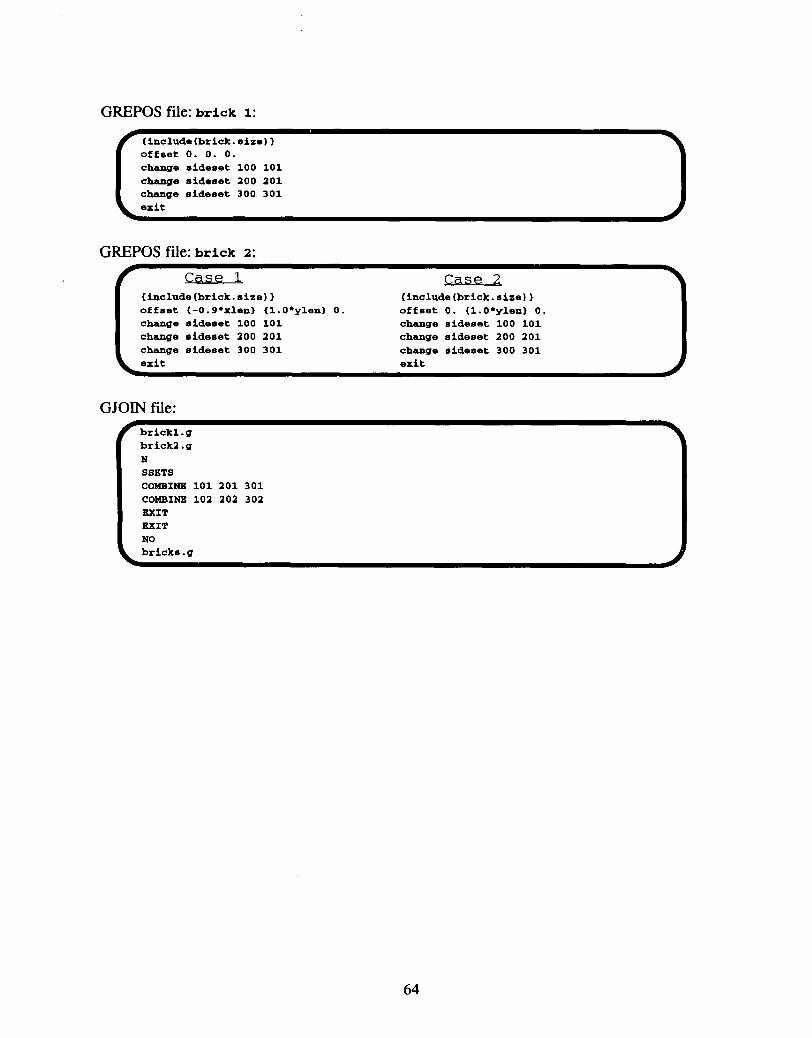
GREPOS file: brick 1:

{include (brick. size) }offset O. 0. 0.

chsnge sldeset 100 101

change sideset 200 201

c-e *ideset 300 301

G~pOSfile:brick 2:

{include(brick. size)) {include(brick. size)}

offset {-O.9*xlen) {1.O*ylen) O. offset O. {1.O*ylen) O.

c-e Sideset 100 101 c-e sideset 100 101change sideeet 200 201 change sideset 200 201

change sideset 300 301 change sideset 300 301

exit

GJOINfiie:

‘brickl.gw

brick2 .g

N

SSETS

COMSINS 101 201 301

COMBINS 102 202 302

XXIT

SXIT

NO

64

PRONT03D input fide:

TITLE

FIXED CONTACT TEST PROB

TERMINATION TIMS = .5X-3

PLOT TIME . .le-5

OUTPUT TIME n .le-5

MATERIAL, 1, ELASTIC, .00074

YOUNQS MODULUS, 30x6

POISONS RATIO, .3333

Em

MATERIAL, 2, XLASTIC, .00074

YOUNQS MODULUS, 30x6


XND

INITIAL VELOCITY NATXRIAL 1 0., 500., 0.

INITIAL VSLOCI~ NATSRIAL 2 0., 0., 0.

PLOT ELEMENT =

PLOT NODAL DISPLACEMENT, REACTION, VELOCITY,

CONTACT SORPACX 101CONTACT SURPACX 102

ACCXLXRATION

BXIT

65

A2.3.2 Pressure Loading of Two Elastic Bodies

FASTQ input:

title

contact chatter

$ {r=.5) (hx=l) (hy=l)

point 1 0. 0.

point 2 {r) O.

point 3 {-r) O.

linelstr1205

line 2 circ 2 3 1 12

line3str3105

region 1 1 -1 -2 -3

point 10 (r) {Q}

point 11 (hx) {o)

point 12 {hx} (by)

point 13 {-hx} {by}

point 14 {-hx) {O}

point 15 {-r} (0)

line 10 str 10 11 0 5

line 11 str 11 12 0 10

line 12 str 12 13 0 20

line 13 str 13 14 0 10

line 14 atr 14 15 0 5

line 15 circ 10 15 1 12

region 2 2 -10 -11 -12 -13 -14 -15

achame 1 C6Sscheme 2 X

sidabc 1 15

aidebc 2 2

sidabc 100 3 1

linebc 11 12

exit

GEN3Dfile:

trenslate 10 1.

66

PRONT03D input fde:

. . . .tt%cle

chatter test problem

termination time .0025

plot time .00001

output time .00001

write restart .001

material 1 elastic .00074

youngs modulus 30e6

poissons ratio .3

end

material 2 elastic .00074

younge madulue

poissons ratio

end

contact surface

pressure 100 50

function 50

0. 0.

.00015 20000.

.01 20000.

end

no displacement

no displacement

exit

30e6

.3

12

1.

y 11

x 11

67

A2.3.3 Buckling of a Shell-like Structures

makefile:

can. g2d: can. fsq can. size

fastq -aprepro -m can. g2d can. faq

can. g: can. g2d can. gen3d can. size

gen3d -aprepro can. g2d can. g <can. gen3d

block.g2d: block.fsq can.size

fastq -aprepro -m block.g2d block.fsq

block.g: block.g2d block.gen3d can.size

gen3d -aprepro block.g2d block.g < block.gen3d

can_block. g: can.g block.g car_block.gjn

gjoin < car_block.gjn

FASTQinputfor can:

.‘ title

self contact test

(include (can.size) )

point 1 0 0

point 2 {rad) O.

point 3 (rad+t) O.

point 4 (-rad) O.

point 5 {-rad-t} O.

line 1 str 2 3 0 {ithick

line 2 circ 2 4 1 {irad)

line 3 str 4 5 0 (Ithick:


region 1 1 -1 -2 -3 -4


line 6 clrc 5 3 1 {irad)

$ half can

region 2 3 -1 -5 -3 -6

aidebc 1 2 5

sidabc 2 4 6

68

FASTQ input for block:v *

title

self contact test problem

{Include(can.size) )

point 1 (rad+e) {-(rad+e))

point 2 (-(rad+e)) {-(rad+e)}

point 3 {-(rad+e)} {rad+e)

point 4 {rad+e} (rad+e)

line 1 str 1 2 0 {isq)

line 2 str 2 3 0 {isq)

line 3 str 3 4 0 {isq}

line 4 str 4 1 0 {isq}

region 1 2 -1 -2 -3 .4

sldebc 1000 1 2 3 d

exit

can. size:

$ $ cylinder rad = (rad=5} t= {t=.2) Int = (lthlck=3} (irad=40)

$ length of cylender (cyllen=15)

.$number of elements in cylinder {icYl=40}

$ block {e = 2} Int= (iSCI = 28}

$ number of elements in block thick {iblkt .5 ) block thicknees {blkt=2.5)

$ block angle {angle=lO)

GEN3D file for can:

{include(can. size))

translate (icyl) (cyllen)

sideset front 4

nodeset back 100

GEN3D file for block:

{include(can.size)}

translate {Iblkt] (blkt)

revolve y {180+angle)

revcen O. 0. 0.

offset O. 0. {tand(angle) *(rad+t)+.01}

sideaet front 3

G.IOINfiie:● ●

Cal.g

block .g

no

ssets

combine 1 2 4

combine 3 1000

exit

exit

no

can_block. gb d

69

PRONT03D input file:

title

self contact test problem

hourglass stiffness .01 .03

TERMINATION TIMS = .004

RBAD RSSTART = .002

WRITS RSSTART = .00005

PLOT TINS = .0001

OUTPUT TINS = .00001

MATSRIAL, 1, BLASTIC plastic, .00074

YOUNUS MODULUS, 301s6


hardening zcdulus O.

yields stress 30000

beta . 1

END

MATERIAL, 2, ELASTIC plastic, .00074

YOUNQS MODULUS, 30E6


hardening modulus O.

yields stress 30000

beta = 1

mm

MATSRIAL, 3, ELASTIC plastic, .00074

YOUNW MODULUS, 30E6


hardening nkxlulus O.

yields atreee 30000

beta . 1

END

contact surface 1

contact surface 3

INITIAL VBIA3CITY MATSRIAL 2 0., 0. -5000.

no dieplacemt x 100

no displacemt y 100

no displacemt z 100

PLOT XLXM13NT .

PLOT NODAL DISPLACSMBNT, VELOCITY, ACCELERATION

plot state . eqpe

EXIT

70

A2.3.4 Cutting of a Steel Pipe

makeflle:fbladel. g2d: bladel. fsq blade .size T

fastq -aprepro -n bladel. g2d bladel. fsq

bladel.g: bladel.g2d blade.size bladel.gen3d

gen3d -aprepro bladel.g2d bladel.g <bladel.gen3d

edge.g2d: edge.fsq blade.nize

faBtq -aprepro -m edge.g2d edge.fsq

e~el.g3: edge.g2d blade.size edgel.gen3d

gen3d -aprepro edge.g2d edgel.g3 < edgel.gen3d

edgal.g31: edgel.g3 edgel.grp blade.eize

grepos -aprepro edgel.g3 edgel.g31 < edgel.grp

edgel.g: edgel.g31 edgell.grp blade.size

grepos -aprepro edgel.g31 edgel.g < edgell.grp

edge2.g3: edge.g2d blade.eize edge2.gen3d

gen3d -aprepro edge.g2d edge2.g3 < edge2.gen3d

edge2.g31: edge2.g3 edge2.grp blade.size

grepos -aprepro edge2.g3 edge2.g31 < edge2.grp

edge2.g: edge2.g31 edge21.grp blade.size

grepos -aprepro edge2.g31 edge2.g < edge21.grp

edge3.g3: edge.g2d blade.size edge3.gen3d


edge3.g31: edge3.g3 edge3.grp blade.eize



grepoa -aprepro edge3.g31 edge3.g < edge31.grp



edge4.g31: edge4.g3 edge4.grp blade.size






edge5.g31: edge5.g3 edge5.grp blade.eize




71

ma.kefile (contd):● ☞blade.g3a bladel.g edgel.g edge2.g edge3.g edge4.g edge5.g blade.gjn

gjoin < blade.gjn

blade.g: blade.g3 blade.grp

grepos -aprepro blade.g3 blade.g < blade.grp

pipel.g2d: pipel.faq blade.size pipe.size

fastq -aprepro -m pipel.g2d pipel.faq

pipel.g3! pipel.g2d blade.size pipe.size plpel.gen3d

gen3d -aprepro pipel.g2d pipel.g3 <pipel.gen3d

pipel.g: pipel.g3 pipel.grp

grepos -aprepro pipel.g3 pipel.g < pipel.grp

pipe2.g2d: pipe2.faq blade.size pipe.size

faetq -aprepro -m pipe2.g2d pipe2.feq

pipe2.g3: pipe2.g2d blade.size pipe.size pipe2.gen3d

gen3d -aprepro pipe2.g2d pipe2.g3 <pipe2.gen3d

pipe2.g: pipe2.g3 pipe2.grp

grepoa -aprepro pipe2.g3 pipe2.g < pipe2.grp

clamp.g2d: clamp.fsq blade.size pipe.size clemp.size

fastq -aprepro -m clamp.g2d cl~.fsq

clamp.g3: clamp.g2d blade.size pipe.size clamp.size

gen3d -aprepro clamp.g2d clamp.g3 <clamp.gen3d

clamp.g: clamp.g3 blade.size clamp.size clamp.grp

grepos -aprepro clamp.g3 clamp.g < cl~.grp

clamp.gen3d

pcut.g: blade.g pipel.g pipe2.g clamp.g

gjoin < pcut.gjn

72

FASTQ input for bladel:

‘title●

pipe cutter blade

{include(blade .elze)}

point 1 -2.594 0.312

point 2 2.716 0.312

point 3 {x3) {y3}

point 4 {x4) {y4}

point 5 {x5} {y5}

point 6 {x6) {Y6}

point 7 {x7} {y7}

point 8 {x8} (Y8)

point 9 {x9) {y9)

point 10 {0.5*(x8+x9)} {y8+0.7’abs (x8-x9)}

point 11 {0.5*(x8+x9)) {y8-O.068)

line 1 str 1 2 0 (3’11)

line 2 str 2 3 0 {4*il} 0.9

line 3 str 3 4 0 (2”11)

line 4 str 4 8 0 (10*I1} 0.8

line 5 clrc 11 8 10 {3’11} 1.17647

line 6 circ 9 11 10 {3’11) 0.85

line 7 str 9 6 0 {1O*I1) 1.25

line 8 str 6 7 0 (3’11}

line 9 atr 1 7 0 (4’11) 0.9

region 1 1 -1 -2 -3 -4 -5 -6 -7 -8 -9

scheme 1 x68

nodebc 200 1

exit

& A

GEN3D file for blade 1:

{include(blade. size))

[

translate {12} {bthick/2.+.002)

nsets back 100

esets front 20

exit

blade. size:

$ {11=1) (12=2) {bthick=O.25)

$ (x3=2.716) (Y3=-2.1715)

$ {x4=1.5) {Y4=-2.286}

$ {x5=0.156) {Y5=-3.63}

$ {x6=-1.0~09) {Y6=-2.4331)

$ (x7=-2.594) (Y7=-2.175)

$ {x8=0.288583) {Y8=-3.497417)

1 $ {x9=0.023417) (Y9=-3.497417)

73

FASTQ input for edge:

pipe cutter blade edge

(include (blade. size) )

point 1 0.002 0.0

point 2 -0.125 0.0

point 3 -0.02 -0.2

point 4 0.002 -0.2165

point 5 0.002 -0.205

line 1 str 1 2 0 {i2)

line 2 str 2 3 0 (2*i2) 0.8

line 3 circ 3 4 5 2

line 4 str 4 1 0 {2*i2) 1.4

region 1 1 -1 -2 -3 -4

scheme 1 X6

nodebc 100 4

sidebc 10 2 3

exit

GEN3Dfileforedge 1:


translate {2*il), {x3-x4)

GREPOS files for edge 1:

{include(blade.size) )

elope left (atan(ebS(y4-y3)/abS(X4-X3) ))

slope right (atan(zbs(y4-y3)/abs(x4-x3) )}

0.0 0. 0.

{-ebs(x4-x3)) 0.0 {-abs(Y3-Y4))

end

{include(blade size)}

revcen 0.0 0.0 0.0

revolve y 90.

offset x {x3) y {y3) z {-bthick/2.0)

GEN3Dfileforedge2:

(include(blade size))

tranzlate {lO*il), {x4-x8) 0.8

74

GREPOS files for edge2:

r {include(blade.size))

offset apline

slope left {aten(abs(y5-y4)/abs(x5-x4) ))

slope right {atan(abs(y5-yd)/abs(x5-xd) ))

0.0 0. 0.

(-abs(x5-x4)) 0.0 (-abs(y4-y5)}

end

exit

r (include(blade.size))

revcen 0.0 0.0 0.0

revolve y 90.


exit

GEN3D file for edge3:

{include(blade. size)}

translate (lO*il), {x9-x6) 1.25

GREPOS files for edge3:

r (include(blade.size))

offset spline

slope left (atan(abs(y6-y5)/abs (x6-x5)))

slope right {atan(abs(y6-y5)/abs (x6-x5))}

0.0 0. 0.

{-ebs(x6-x5)) 0.0 {abs(y5-y6))

end

exit

{include(blade. size)}

revcen 0.0 0.0 0.0

revolve y 90.

offset x {x9) y {y9) z (-bthick/2.0)

GEN3Dfileforedge4:

{include(blade size))

translate {3*il}, {x6-x7}

75

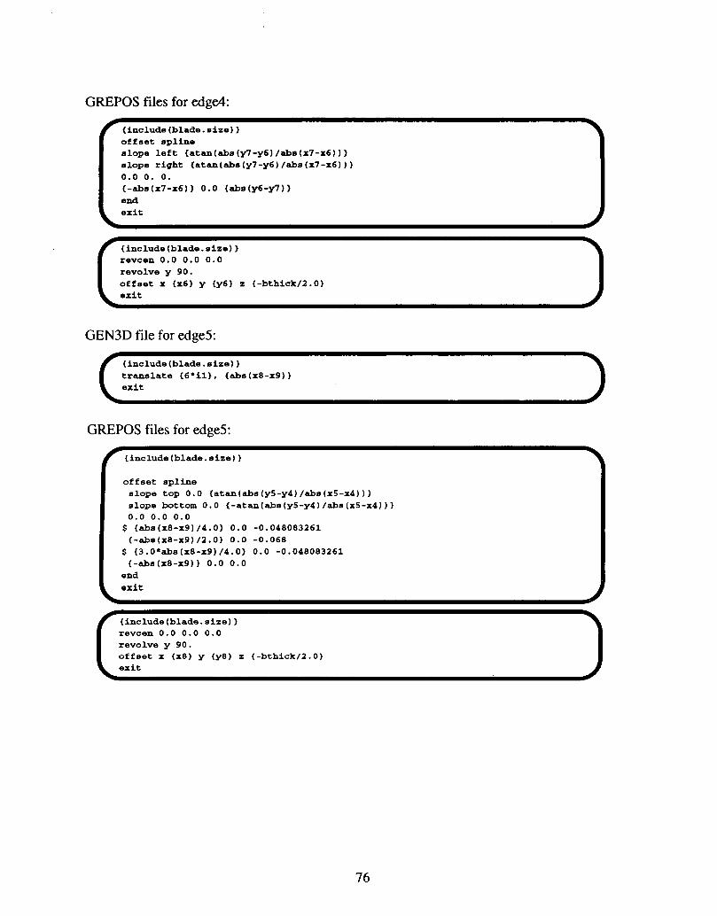
GREPOS files for edgwl:


slope left {atan(abs(y7-y6)/abs(x7-x6) )}

slope right {atan(abs(y7-y6)/abs (x7-x6)))

0.0 0. 0.{-sbs(x7-x6)} 0.0 {sbs(Y6-Y7))end


revcen 0.0 0.0 0.0

revolve y 90.

offset x {x6} y (y6) z (-bthick/2.0)

GEN3D file for edge5:

(include(blade size)}

translate {6*il), {abs(x8-x9))

GREPOSfilesforedge5:

~{include(blade. eize))*

offset spline

slope top 0.0 {atan(abs(y5-y4)/abs (X5-X4)))

slope bottom 0.0 {-atan(abs(y5-y4)/abs (x5-x4)))

0.0 0.0 0.0

$ (sbs(x8-x9)/4.0} IJ.O -0.048083261(-abs(x8-x9)/2.0) 0.0 -0.068

$ {3.0*abs(x8-x9)/4.0) 0.0 -0.048083261

{-abs(x8-x9)} 0.0 0.0

end

exit


revcen 0.0 0.0 0.0

revolve y 90.


76

GJOIN file for blade:

edgel. g

combine .000001

combine exit

exit

yes

edge2 .g

combine .000001

combine exit

exit

yea

edge3. g

combine .000001

combine exit

exit

yes

edge4. g

combine .000001

combine exit

exit

yea

edge5. g

combine .01

combine exit

exit

no

blade.g3

GREPOS file for blade:

foffset y -0.064

exit )

77

FASTQ input for pipel:. .

titlepipe

{include(pipe. size)}(include(blade. size)}

point 1 {x5} (Y5 - (bthick/2.)/tan(3.14159*30. /180.) - pr - pt)

point 2 (x5) (Y5 - (bthick/2.)/tan(3.14159’30. /180.) - pt }

point 3 {x5) (Y5 - (bthick/2.)/tan(3.14159*30. /180.) }

point 4 {x5) {y5 - (bthick/2.)/tan(3.14159*30. /180.) - 2*pr - pt )

point 5 {x5) {ys - (bthick/2.)/tan(3.14159*30. /180.) - 2*pr -2’pt)

line 1 str 2 3 0 {ithick)


line 3 str 4 5 0 (ithick)

line 4 circ 3 5 1 (irad}

line 5 circ 4 2 1 {irad}

line 6 circ 5 3 1 {irad}

region 1 2 -1 -2 -3 -4

region 2 3 -1 -5 -3 -6

exit

pipe. size:

$ {ithkk=4} (irad=50) {pr=l.0335) {pt=O.154}

$ {ithick2=2) {irad2=25]

$ {Rlength=l.5} {i3=16}

$ {Rlen@h2=3.5) {i4=12}

GEN3D file for pipel:r

{include(blade size))*

{include(pipe size))

translate (13) {plength/2.) 1.05

nsets front 100

ssets back 400

exit

I d

78

GREPOS file for pipel :FASTQ input for pipe2:

{include (blade. size) )

revcen (x5) 0.0 0.0

revolve y 180

offeet x 0.00001 z (-bthick/2.+0.0001)

\ wF ●

title

pipe

(include(pipe size))


point 1 {x5} (Y5 - (bthick/2.)/tan(3.14159*30. /180.) - pr - pt)

point 2 {x5} {ys - (bthick/2.)/tan(3.14159*30. /180.) - pt )

point 3 {x5} {y5 - (bthick/2.)/tan(3.14159*30. /180.) }

point 4 {x5) {Y5 - (bthick/2.)/tan(3.14159*30. /180.) - 2*pr - pt )

point 5 {x5) (Y5 - (bthick/2.)/tan(3.14159*30. /180.) - 2*pr -2’pt}

line 1 etr 2 3 0 {ithick2)

line 2 circ 2 4 1 {irad2)

line 3 str 4 5 0 {ithick2}

line 4 circ 3 5 1 (irad2}

line 5 circ 4 2 1 (irad2}

line 6 circ 5 3 1 (irad2)

region 1 4 -1 -2 -3 -4

region 2 5 -1 -5 -3 -6

exit

k 4

GEN3D file for pipe2:

(include(blade. size)}

{include(pipe. size))

tramslate {i4) (plength2) 1.08

aseta front 401

GREPOS file for pipe2:v


(include(pipe.size) )

revcen (x5} 0.0 0.0

revolve y 180

offset x 0.00001 z {-bthick/2.+0.0001+plength/2.}

exit

k 4

79

FASTQ input for clamp:-.P T

title

clamp

{include (pipe. eize) }

{include (blado. size) )

{include(clamp. size)}

point 1 -4.0 (Y5 - (bthick/2.)/tan(3.14159’30. /180.) - 2“pr -2”pt)

point 2 4.0 (y5 - (bthick/2.)/tan(3.14159*30. /180.) - 2*pr -2*pt)

point 3 4.0 (Y5 - (bthick/2.)/tan(3.14159*30. /180.) - 2*Pr -2’pt - cheight)

point 4 -4.0 {y5 - (bthick/2.)/tan(3.14159*30. /180.) - 2*pr -2*pt - cheight)

linelstr1208

line2etr2302

line3str3408

line4str4102

region 1 1 -1 -2 -3 -4

nodebc 300 3

sidebc 30 1

exit

k d

clamp.size:

$ {cthick=O.5} {coffset=O.31}

GEN3Dfileforclamp:


{include(pipe. size))

{include(clemp. size))

translate 2 {cthick}

sset back 31

GREPOSfilefor clamp:

(include(blade. size)}

{include(clemp. size))

offset z (cthick+coffset-bthick/2.)

80

GJOIN file for blade, pipe, and clamp:

‘lblade.g+

pipel.g

no

exit

yee

pipe2. g

no

exit

yea

Clamp.g

no

exit

no

pcut .g

PRONT03D input file:

TITLE

Pipe Cutting Simulation

$hourglaas stiffness 0.01 0.03

TERMINATION TIME = 4.B-3

PI.KITTIMS . 4.e-5

OUTPUT TIMS = 4.e-5

write restart = 8.e-5

function 1

0.0 1.0

1.0 1.0

end


YOUNGS MODULUS, 30E6


END

MATERIAL, 2, plh strength , .00074


POISONS RATIO, .3

yield stress, 38.8e3

hardening constant 93.6e3

hardening exponent 0.4539

luders strain 0.021

failure value 1.27

decay conetant 0.7

BND

MATERIAL , 3, plh etrength , .00074


POISONS RATIO, .3

yield strese, 38.8e3



luders strain 0.021

failure value 1.27

decay constant 0.7

END

PRONT03D input fde (contd):r

NATS3UAL, 4, plh strength , .00074

YOUNUS MODULUS, 30B6

POISONS RATIO, .3

yield stress, 38.8e3



luders strain 0.021

failure value 1.27

decay constant 0.7

END

NATSRIAL, 5, plh etrength , .00074

YOUNGS NODULUS, 30B6

POISONS RATIO, .3

yield stress, 38.8e3hardening constant 93.6e3hardening exponent 0.4539luders strain 0.021failure value 1.27decay constant 0.7

mm

death 2 decay min 0.1

death 3 decay m.in 0.1

prescribed VBLOCITY y 200 1 -1187.5

INITIAL VSLOCITY MATSRIAL 1 0. -1187.5 0.

no displacement z 100

no displacement y 300

PLOT HJQ4SNT = vonm.ises, pressure

plot state . eqpe

PLoT NODAL DISPLACXMSNT, REACTION, VELOCITY,

7

AccmAsRATIoN

contact surface 400 401 fixed

CONTACT material 1

CONTACT material 2

CONTACT material 3

SXIT

82

A2.3.5 Elastic-Plastic Bar Impacting Bricks

makefile:

bricks.g2d: bricks.fsq 1

fantq -aprepro -m bricks.g2d -- bricks.fsq

bricks.g: bricks.g2d bricks.gen3d

gen3d bricks.g2d bricks.g <bricks.gen3d

bricks.gx: bricks.g

exoxdr bricke.g bricks.gx

wall.g2d: wall.fsq

fastq -m wall.g2d -- wall.faq

wall.g: wall.g2d wall.gen3d

gen3d wall.g2d wall.g <wall.gen3d

brick_wall.gx: brick_wall.g

exoxdr brick_wall.g brick_wall.gx

rod.g2d: rod.fsq

fastq -m rod.g2d -- rod.faq

rod.g: rod.g2d rod.gen3d

gen3d rod.g2d rod.g <rod.gen3d

brick_wall.g: bricks.g wall.g rod.g

gjoin < brick_wall.gjn .A

83

FASTQ file for bricks:

TITLE

STSEL ROD EITTINQ BRICRS

$ {e = .005}

POINT 1 {0. +e} (0. +e)

POINT 2 {I.-e} {0. +e}

POINT 3 (I.-e) {.5-e)

POINT 4 (0.+e} (.5-e}

LINB1STR1201O

LINs2sTR2305

LINB3STR3401O

LINE 4 STR4 1 0 5

RRQION 1 1 -1 -2 -3 -4

POINT 11 {1.+e} {0.+e}

POINT 12 {2.-e} (0.+e}

POINT 13 (2.-e) {.5-e)

POINT 14 {1.+e} {.5-e)

LINE 11 STR 11 12 0 10

LINE 12 STR 12 13 0 5

LINE 13 STR 13 14 0 10

LINE 14 STR 14 11 0 5

RBQION 11 1 -11 -12 -13 -14

POINT 21 {2.+e) {0.+e}

POINT 22 {3.-e} {0.+e)

POINT 23 {3.-e) {.5-e}POINT 24 {2.+e) {.5-e)

LINE 21 STR 21 22 0 10

LINE 22 STR 22 23 0 5

LINS 23 STR 23 24 0 10

LINE 24 STR 24 21 0 5

REGION 21 1 -21 -22 -23 -24

.$SECOND ROW

POINT 101 {0.+e} {.5+e}

POINT 102 {.5-e) {0.5+e}

POINT 103 {.5-e) {I.-e)

POINT 104 {0.+e) (l.-e)

LINE 101 STR 101 102 0 5

LINE 102 STR 102 103 0 5

LINE 103 STR 103 104 0 5

LINE 104 STR 104 101 0 5

REGION 101 1 -101 -102 -103 -104

POINT 111 (.5+e} {.5+e}

POINT 112 {1.5-e} (.5+e}

POINT 113 {1.5-e) {l.-e)

POINT 114 (.5+e) {I.-e}

LXNB 111 STR 111 112 0 10

LINE 112 STR 112 113 0 5

LINS 113 STR 113 114 0 10

LINE 114 STR 114 111 0 5

RBCION 111 1 -111 -112 -113 -114

POINT 121 {1.5+e) {.5+e}

POINT 122 {2.5-e} {0.5+e)

POINT 123 {2.5-e) {l.-e)

POINT 124 {1.5+e} {l.-e)

LINE 121 STR 121 122 0 10

LINE 122 STR 122 123 0 5

LINE 123 STR 123 124 0 10

LINE 124 STR 124 121 0 5

REGION 121 1 -121 -122 -123 -124

POINT 131 {2.5+e) {.5+e)

POINT 132 {3.O-e} (0.5+e}

POINT 133 {3.O-e} {l.-e)

POINT 134 {2.5+e} {l.-e}

LINE 131 STR 131 132 0 5

LINE 132 STR 132 133 0 5

LINE 133 STR 133 134 0 5

LINE 134 STR 134 131 0 5

RSGION 131 1 -131 -132 -133 -134

$ TNIRD ROW

POINT 201 {0.+e) {1.+e)

POINT 202 {l.-e} {1.+e)

POINT 203 {l.-e) {1.5-e)

POINT 204 (0.+e) {1.5-e}

LINE 201 STR 201 202 0 10

LINE 202 STR 202 203 0 5

LXNB 203 STR 203 204 0 10

LINS 204 STR 204 201 0 5

RSGION 201 1 -201 -202 -203 -204

POINT 211 {1.+e) {1.+e)

POINT 212 (2.-e) (1.+e)

POINT 213 {2.-e} (1.5-e)

POINT 214 {1.+e) {1.5-e}

84

FASTQ file for bricks (contd):

LINS 211 STR 211 212 0 10 REGION 321 1 -321 -322 -323 -324

LINE 212 STR 212 213 0 5

LINE 213 STR 213 214 0 10

LINE 214 STR 214 211 0 5

REGION 211

POINT 221

POINT 222

1 -211 -212 -213 -214

2.+e} {1. +e)

3.-e} {1. +e)

POINT 223 {3.-e} (1.5-e}POINT 224 {2.+e} {1.5-e)

LINB 221 STR 221 222 0 10

LINS 222 STR 222 223 0 5

LINE 223 STR 223 224 0 10

LINE 224 STR 224 221 0 5

RSGION 221 1 -221 -222 -223 -224

PoINT 331 {2.5+e} {1.5+e)

POINT 332 {3.O-e) {1.5+e)

POINT 333 {3.O-e) {2.-e)

POINT 334 {2.5+e) {2.-e}

LINS 331 STR 331 332 0 5

LINB 332 STR 332 333 0 5

LINB 333 STR 333 334 0 5

LINS 334 STR 334 331 0 5

REGION 331 1 -331 -332 -333 -334

$ FIFTH ROW

POINT 401 {0.+e) {2.+e}POINT 402 {l.-e} {2. +e)

POINT 403 (I.-e) {2.5-e)

POINT 404 {0.+e) {2.5-e)

$ FOURTS ROW

POINT 301 {0.+e)

POINT 302 {.5-e}

POINT 303 {.5-e}

POINT 304 {0.+e}

LINB 301 STR 301

LINS 302 STR 302

LINE 303 STR 303

LINB 304 STR 304

{1.5+e}

(1.5+e)

{2.O-e}

{2.O-e)

302 0 5

303 0 5

304 0 5

301 0 5

RKGION 301 1 -301 -302 -303 -304

POINT 311 {.5+e} (1.5+e)

POINT 312 (1.5-e} {1.5+e)

POINT 313 (1.5-e) {2.-e}

POINT 314 (.5+e) {2.-e)

LINE 311 STR 311 312 0 10

LINE 312 STR 312 313 0 5

LINS 313 STR 313 314 0 10

LINE 314 STR 314 311 0 5

RSGION 311 1 -311 -312 -313 -314

POINT 321 {1.5+e} (1.5+e)

POINT 322 {2.5-e) (1.5+e)

POINT 323 {2.5-e} {2.-e}

POINT 324 {1.5+e) {2.-e}

LINE 321 STR 321 322 0 10

LINE 322 STR 322 323 0 5

LINS 323 STR 323 324 0 10T.TNR ~2A .STR ~2A 791 (l ~

LINS 401 STR 401 402 0 10

LINS 402 STR 402 403 0 5

LINB 403 STR 403 404 0 10

LINE 404 STR 404 401 0 5

REGION 401 1 -401 -402 -403 -404

POINT 411 {1.+e) {2.+e)

POINT 412 (2.-e) {2. +e)

POINT 413 {2.-e} {2.5-e)

POINT 414 {1.+e} {2.5-e)

LINS 411 STR 411 412 0 10

LINE 412 STR 412 413 0 5

LINB 413 STR 413 414 0 10

LINB 414 STR 414 411 0 5

REGION 411 1 -411 -412 -413 -414

POINT 421 {2.+e} {2. +e}

POINT 422 {3.-e) {2. +e}

POINT 423 (3.-e} {2.5-e]

POINT 424 {2.+e} {2.5-e)

LINS 421 STR 421 422 0 10

LINS 422 STR 422 423 0 5

LINB 423 STR 423 424 0 10

LINE 424 STR 424 421 0 5

REGION 421 1 -421 -422 -423 -424

EXIT

85

GEN3D file for bricks:

translate 3 .6

FASTC) file for wall:

~*

wall

point 1 5.5 0.point 2 5.85355 .35355

point 4 .5 5.

point 3 .85355 5.35355

line lstr 1205

line 2 str 2 3 0 70

line3s.tr3405

line 4 str 4 1 0 70

region 1 3 -1 -2 -3 -4

exit

GEN3Dfileforwall:

translate 9 1.5

offset 0.05 0.05 .5

FASTQ file for rod:

brick wall example

!$STEEL ROD

POINT 500 1.25 0.

POINT 501 1.75 0.

POINT 502 1.75 -.5

POINT 503 1.25 -.5

LINE 501 STR 500 501 0 5

LINE 502 STR 501 502 0 5

LINS 503 STR 502 503 0 5

LINS 504 STR 503 500 0 5

REGION 500 2 -501 -502 -503 -504

SXIT

GEN3Dfilefor rod:

translate 30 5

offset O. 0. 3.

86

GREPOS file for bricks, wall, and rod:.,,

bricks.g

wall.g

no

exit

yes

rod. g

noP exit

i no

brick_wall.g

PRONT03Dinput file:

title

MULTI-BOBY CONTACT test problem

TMU41NATION TIMB = .0005

PLOT TIM = .00001

OUTPUT TIMB = .00001

MATBRIAL, 1, ELASTIC, .00074

YOUNCJS MODULUS, 30E6


END


YOUNGS MODULUS, 30E6


END

MATBRIAL, 3, ELASTIC plastic, .0005

YOVNGS MODULUS, 16X6


hardening modulus 1000.

beta = 1

yield stress = 10000.

END

INITIAL VBLOCITY MATSRIAL 2 0. , 2500. , 0.

PLOT ELEMBNT =

PLOT NODAL DISPLACEMENT, VSLOCITY, ACCELERATION

CONTACT MATERIAL 1

CONTACT MATSRIAL 2

CONTACT MATERIAL 3

BXIT

87

A2.3.6 Forging of a Copper Billet

FASTQ file:

RIVET PROBLKM FOR CONTACT SURPACB CHECK

POINT 1 0.0 0.0

POINT 2 2.0 0.0

POINT 3 2.2 0.0

POINT 4 0.0 0.2

POINT 5 2.0 0.2

POINT 6 2.2 0.2

POINT 7 2.0 2.95

POINT 8 2.2 3.0

POINT 9 4.0 3.0

POINT 10 2.0 3.2

POINT 11 2.25 3.2

POINT 12 4.0 3.2

POINT 13 0.0 0.2

POINT 14 1.75 0.2

POINT 15 1.75 6.2

POINT 16 0.0 6.2

POINT 17 0.0 6.2

POINT 18 4.0 6.2

POINT 19 4.0 7.2

POINT 20 0.0 7.2

POINT 21 2.25 3.0

POINT 22 2.20 2.95

POINT 23 2.25 2.95

LINE 1 STR1 3 0 1

LINB2STR32201

LINE 3 STR 21 9 0 1

LINB4STR4501

LINB 5 STR5 7 0 1

LINE 6 STR 11 12 0 1

LINB 7 STR1 4 0 1

LINB 8 STR 5 3 0 1

LINE 9 STR 8 10 0 1

LINB 10 STR 9 12 0 1

LINE 13 STR 13 14 0 20

LINS 14 STR 14 15 0 80

LINE 15 STR 16 15 0 20

LINB 16 STR 13 16 0 80

LINE 17 STR 17 18 0 1

LINB 18 STR 18 19 0 1

LINE 19 STR 20 19 0 1

LINB 20 STR 17 20 0 1

LINB 21 CIRC 21 22 23 45LINB 22 CIRC 11 7 23 45

LINB 23 STR 7 22 0 1

LINB 24 STR 21 11 0 1

REGION 1 1 -1 -8 -4 -7

REGION 2 1 -2 -23 -5 -8

REGION 3 1 -3 -10 -6 -24

RBGION 4 2 -13 -14 -15 -16

RB1310N 5 3 -17 -18 -19 -20

REGION 6 1 -21 -24 -22 -23

NODBBC 3 1 2 3 4 5 6 21 22

NODXBC 1 16 17 18 19 20

NODEBC 2 17 18 19 20

SIDBBC 100 4 5 6 22

SIDBBC 200 13 14 15

SIDEBC 300 17

SIDEBC 400 14 15

(\ BXIT .

88

SANTOS2D input file:

TITLE

RIVET PROBLEM - CRECK FOR CONTACT SURFACES

AXISYMMBTRIC

STEP CONTROL

500 1.

END

OUTPUT TIMB

10 1.

END

PLOT TIME

5 1.

XND

TIME STEP SCALE = 0.75

MINIMUM DAMPINQ FACTOR = .8

RESIDUAL TOLERANCE, 0.5MAXIMUM TOLBRANCB, 100.

MAXIMUM ITERATIONS, 2000

INTERMEDIATE PRINT, 10

PLOT NODAL = DISPLACEMENT

PLOT STATE = EQPS

PLOT ELXMENT = VONMISES, PRESSURE, STRESS, STRAIN

FUNCTION, 1

0.0,0.0

1.0,1.0

END

MATBRIAL, 1, BLASTIC, 1.

YOUNGS MODULUS = 30.x6

POISSONS RATIO = 0.3END

MATERIAL, 2, EP POWER HARD, 1.

YOUNGS MODULUS = 17.0E+6

POISSONS RATIO = 0.35

SARDENINC3 CONSTANT = 50.0E+3

SARDENINQ EXPONENT = .31

YIELD STRESS = 15.5E+3

LUDER STRAIN = 0.0

END

MATERIAL, 3, ELASTIC, 1.

YOUNQS MODULUS = 30.E+6,

POISSONS RATIO = 0.3

END

CONTACT SURFACE, 100, 200, 0., 1.E-10

CONTACT SURFACE, 300, 400, 0., 1.B-10

NO DISPLACEMENT, X, 3

NO DISPLACBMBNT, Y, 3

NO DISPLACEMENT, X, 1

PRESCRIBED DISPLACEMENT, Y, 2, 1, -2.5

EXIT

89

DISTRIBUTION:

1 Dr. R. T. AllenPacifica TechnologyP.O. BOX 148Del Mar, CA 92014

3 Anatech International Corp.5435 Oberlin DriveSan Diego, CA 92121Attn: Dr. R. A. Dameron

Dr. R. S. DunhamDr. Joe Rashid

Prof. S. AtluriCenter for the Advancement of

Computational MechanicsSchool of Civil EngineeringGeorgia Institute of TechnologyAtlanta, GA 30332

Dr. Ali S. ArgonDept. of Mechanical EngineeringMassachusetts Institute of

TechnologyCambridge, MA 02139

Dr. William E. BachrachAreojet Research Propulsion Inst.P. O. BOX 13502Sacramento, CA 95853-4502

Mr. Ken Bannister

USA Ballistic Research LabSLCBR-IB-MAberdeen Proving Grounds, MD21005-5066

3 Battelle505 King AvenueColumbus, OH 43201-2693Attn: Mr. R. Douglas Everhart

Dr. Michael L. FisherMr. Charles R. Hargreaves

Prof. T. BelytschkoDepartment of Civil EngineeringNorthwestern UniversityEvanston, IL 60201

Mr. Winy BenzUniversity of ArizonaSteward ObservatoryTucson, AZ 85321

Mr. Naury K. BirnbaumCentury Dynamics Incorporated7700 Edgewater Dr., Suite 626Oakland CA 94621

Mr. Akif O. BolukbasiMcDonnell Douglas Helicopter

Company5000 East McDowell RoadMesa, AZ 85205-9797

Dr. Kenneth W. BrownComputer Aided Engineering

Associates, Inc.398 Old Sherman Hill Rd.Woodbury, CT 06798

Mr. Malcolm BurgessAEA Transport Technology205/B71 Winfrith Technology CentreDorchester, Dorset DT2 8DHUnited Kingdom

Mr. Mark CampbellPASTDCO1248 Princeton N.E.Albuquerque, NM 87106

Dr. Tom CanfieldArgonne National Laboratories9700 S. Cass Ave CTD/221Argonne, IL 60439-4844

Mr. Ted CarneyAdvanced Sciences Inc.6739 Academy Road N.E.Albuquerque, NM 87109

Mr. Tien S. ChouEG&G MoundP.O. Box 3000Miarnisburg, OH 45343

Mr. Chuck CharmanGA TechnologiesP.O. BOX81608San Diego, CA 92138

Mr. Ken K. ChipleyMartin Marietta Energy SystemsP.O. BOX2009Oak Ridge, TN 37831-8053

Mr. Ken P. ChongDept. of Civil EngineeringUniversity of WyomingLaramie, WY 82071

Dr. S. C. (Tony) ChouU.S. Army Materials Technology LabSLCMT-BMWatertown, MA 02172-0001

Mr. Dwight ClarkMail Stop 281Morton Thiokol Corp.P. O. BOX524Brigham City, UT 84302

Mr. Gregory CliffordCray Research Park655E Lone Oak DriveEagan,MN55121

Mr. Gerald CollingwoodMorton Thiokol, Inc.Huntsville, AL 35807-7501

Mr. David L. ConoverSwanson Analysis Systems, Inc.P. O. BOX65Houston, PA 15342-0065

Prof. Steven M. CramerUniversity of Wisconsin2266 Engineering Building1415 Johnson DriveMadison, WI 53706

Mr. Steven CrouchGeoLogic Research, Inc.1313 Fifth St. SE, Suite 226Minneapolis, MN 55414

Dr. Ian CullisXTZ DivisionRoyal Armament R&D

EstablishmentFort I-EdsteadSevenoaks, KentUnited Kingdom

Mr. Peter CundallITASCA Consulting Group, Inc.1313 Fifth Street, S.E.Minneapolis, MN 55414

Mr. Richard E. DanellResearch OfficerCentral Research LaboratoriesBHP Research& New TechnologyP.O. Box 188Wallsend NSW 2287Australia

Mr. William A. DanneStrategic Systems Division, MS#50Teledyne Brown EngineeringP.O. Box 07007Huntsville, AL 35807-7007

Dr. C. S. DesaiDept. of Civil Eng. & Eng. Mech.The University of ArizonaTucson, AZ 85721

Mr. Ramji DigumarthiOrg. 8111, Bldg. 157 -Lockheed MSDP.O. Box 3504Sunnyvale, CA 94088-3504

Prof. Robert Dodds, Jr.Department of Civil Engineering3140 Newmark Laboratory, MC-250University of Illinois at UrbanaUrbana, IL 61801-2397

Dr. Arlo FossumRE/SPEC Inc.BOX725Rapid City, SD 57709

Dr. Russel GarnsworthyCRA Advanced Tech DevelopmentG.P.O. BOX384DMelbourne 3001, Australia

Prof. Lorna GibsonDepartment of Civil EngineeringRoom 1-232Massachusetts Institute of


2 Goodyear Technical CenterP.O. Box 3531Akron, OH 44309-3531Attn: Mr. Loren K. Miller

Mr. David Wismer, D/410F

Dr. Gerry GoudreauMethods Development GroupMechanical Engineering DepartmentLawrence Livermore National LabLivermore, CA 94550

Prof. O. Hayden Griffin, Jr.Dept. of Eng. Science & MechanicsVirginia Polytechnic Institute andState UniversityBlacksburg, VA 24061-0219

2 Grumman Corporate TechnologyBethpage, NY 11714-3580Attn: Dr. John M. Papazian

Dr. Allan B. Pifko

Mr. H. L. HassenpflugB&W Fuel CompanyP.O. Box 109353315 Old Forest RdLynchburg, VA 24501

5 Hibbitt, Karlsson & Sorrensen, Inc.100 Medway St.Providence, RI 02906Attn: Dr. David Hibbitt

Dr. Joop NagtegaalDr. D. P. FlanaganDr. L. M. TaylorDr. W. C. Mills-Curran

Mr. Richard HilsonM/s 4009GTE Government SystemsCorporationP.O. BOX7188Mountain View, CA 94039

Mr. Douglas HolzhauerRome Air Development CenterGriffiss AFB, NY 13441

Dr. William HufferdUnited TechnologiesChemical Systems DivisionP.O. Box 50015San Jose, CA 95150-0015

Prof. T. J. R. HughesDept. of Mechanical EngineeringStanford Universitypalo Alto, CA 94306

Mr. James P. JohnsonRm L 120, CPC Analysis Dept.General Motors Corp. Engineering

Center30003 Van Dyke AvenueWarren, MI 48090-9060

Mr. Jerome B. JohnsonUSACRRELBuilding 4070Ft. Wainwright, AK 99703

Mr. Ken JohnsonTheoretical and Applied Mechanics

GroupBattelle Pacific Northwest

LaboratoriesP.O. Box 999Richland, WA 99352

Dr. Gordon R. JohnsonHoneywell, Inc.5901 S. County Rd. 18Edina, MN 55436

Mr. James W. JonesSwanson Service Corporation18700 Beach Blvd.Suite 200-210Huntington Beach, CA 92648

Mr. Sheldon JonesKaman SciencesP.O. BOX 7463Colorado Springs, CO 80933-7463

Mr. G. A. KaeppFord Motor CompanyP.O. Box 2053, Room 2019Dearborn, MI 48124

Dr. David W. KeckCONVEX Computer CorporationP.O. BOX833851 M.S. MARRichardson, TX 75083-3851

Mr. Gary KetnerApplied Mechanics and StructuresBattelle Pacific Northwest

LaboratoriesP.O. Box 999Richland, WA 99352

Dr. Sam KeyRE/SPEC Inc.4775 Indian School NE, Suite 300Albuquerque, NM 87110-3827

Prof. Raymond D. KriegEngineering Science and Mechanics301 Perkins HallUniversity of TennesseeKnoxville, TN 37996-2030

Mr. Don D. KunardAnalytical Systems Engineering

Corp.1725 Jefferson Davis Hwy, Suite212Arlington, VA 22202

Mr. Brett LewisAPTEK1257 Lake Plaza DriveColorado Springs, CO 80906-3578

Norman A. LindseyMCAE Technical MarketingCONVEX Computer CorporationP. O. BOX833851 M.S. MARRichardson, TX 75083-3851

Mr. Trent R. LoganRockwell International Corp.P.O. BOX 92098Los Angeles, CA 90009

/7

.f

f

,

34 Los Alarnos National LaboratoryLOSAklIllOS, NM 87545Attn:

J. Hopson, T3, MS B216R. Hill, P15, MS D44J. P. Hill,WX-11, MS C931D. J. Sandstorm, MST-DO, MSG756K. A. Meyer, X-3 MS F663W. A. Cook, N-6, MS K557P. T. Maulden, N-6, MS K557J.J.Ruminer,WX-11, MSC931S. P. Girrens, MEE- 13, MS J576J. L. Fales, MEE-13, MS J575J. D. Allen, MEE-4, MS G787

D. A. Rabem, MEE-4, MS G787M. W. Burkett, MEE-4, MS G787J. H. Fu, MEE-4, MS G787P. R. Romero, MEE-4, MS G787P.S. Follansbee, MST-DO,MS G756D. Mandell, X-3, MS F663R. F. Davidson, N-6, MS K557J. N. Johnson, N-6, MS K557J. K. Dienes, N-6, MS K557S. Marsh, N-6, MS K557L. H. Sullivan, N-6, MS K557D. L. Jaeger,WX-11, MS K557C. A. Anderson, MEE-13, MS J576J. G. Bennett, MEE-13, MS J576T. A. Butler, MEE- 13, MS J576D. C. Nelson, MEE-4, MS G787R. B. Parker, MEE-4, MS G787M. W. Lewis, MEE-4, MS G787E. S. Idar, MEE-4, MS G787B. M. Wheat, MEE-4, MS G787F. Guerra, WX- 11, MSC931C. Wingate, MS F645B. Stellingwerf, MS F645

Dr. Jack MaisonEngineering Cybernetics, Inc.1856 Lockhill Selma Rd, Suite 105San Antonio, TX 78213

Mr. Joseph MartiHamilton Standard Division of

United TechnologiesM/S 1-3-BC52One Hamilton RoadWindsor Locks, CT 06096-1010

Mr. Darin McKinnisNASA Pyrotechnics Group, MS EP5LBJ Space CenterHouston, TX 77058

Mr. Craig MillerUnit 973Neutron Devices DepartmentGeneral Electric CompanyP.O. BOX2908Large, FL 34294-2908

2 Lockheed Missiles and Space Co.P. O. Box 3504Sunnyvale, CA 94088-3504Attn:

Mr. J. J. Murphy, 59-22 B/580Mr. Brian M.Cuthbert,81-12 B/157

Prof. V. D. MurtySchool of EngineeringUniversity of Portland5000 N. Willamette Blvd.Portland, OR 97203

2 Naval Surface Warfare Center10901 New Hampsure Ave.Silver Spring, MD 20903-5000Attn:

Mr. Hans Mair, Code R14Mr. Andrew Wardlaw Jr. Code R44

2 Naval Research LabMaterials Science & TechnologyBuilding 28, Code 63864555 Overlook Avenue SWWashington, DC 20375-5000Attn: Mr. Luther D. Flippen

Dr. Carl Dyka

Dr. R. E. Nickellc/o Anatech International Corp.5435 Oberlin DriveSan Diego, CA 92121

Mr. Dean NormanWaterways Experiment StationP.O. BOX631Vicksburg, MS 39180

2 Office of Naval ResearchStructural Mechanics Div. (Code 434)800 N. Quincy StreetArlington, VA 22217Attn: Dr. Rembert Jones

Dr. Alan S. Kushner

Mr. Shane R. PageAlbuquerque Valve & FittingCompany2451 Alamo S.E.Albuquerque, NM 87106

Dr. Robert PardueMartin Marietta, MS 2Y-12 Plant, Bldg. 9998Oak Ridge, TN 37831

Dr. T. Kim ParnellFailure Analysis Associates, Inc.P.O. Box 3015Menlo Park, CA 94025

Dr. Philip A. PfundBabcock & WilcoxP.O. BOX271Barberton, OH 44203

Mr. Mitchell R. PhillabaumMonsanto Research Corp.MRC-MOUNDMiamisburg, OH 45342

4 Phillips Laboratory (AFSC)Kirtland AFB, NM 87117-6008Attn:

Firooz Allahdadi, PLAVSSDDavid Amdahl, PL/WSSDDavid Medina, PL/WSSDDavid H. Hilland, PLAVSSH

3 POD Associates, Inc.2309 Renard Pl, Suite 201Albuquerque, NM 87106Attn: Mr. Dale R. Atkinson

Mr. Steven F. RiecoDr. Alan J. Watts

2 Pratt& Whitney Aircraft400 Main St.East Hartford, CT 06108Attn: John Cowles, MS 118-38

Mick Bruskotter, MS 114-38

Dr. Harold E. ReadS-CubedP.O. BOX 1620La Jolla, CA 92038-1620

Dr. Douglas ReederHardening Technology Dept.General Research Corp.P.O. BOX6770Santa Barbara, CA 93160-6770

Prof. J. A. ReuscherTexas A & MDept. of Nuclear EngineeringCollege Station, Texas 77843

2 Reynolds Metals Company1941 Reymet RoadRichmond, VA 23237Attn: Mr. Stephen P. Sunday

Mr. Armand Beaudoin

Mr. J. S. (Gus) RiceCaterpillar Inc. Technical CenterDivision 927P.O. BOX 1875Peoria, IL 61656-1875

Mr. Samit RoyDept. of Engineering MechanicsSouthwest Research InstituteP.O. Drawer 28510San Antonio, TX 78284

R. G. Sauv6Applied Mechanics SectionMechanical Research DepartmentOntario Hydro700 University AvenueC26Toronto, Ontario M5G 1X6Canada

Mr. Donald W. SandidgeAMSMI-RLAU.S. Army Missile CommandRedstone Arsenal, AZ 35898-5247

Mr. Steven SauerKtech Corporation901 Pennsylvania Ave NEAlbuquerque, NM 87110

Mr. Martin Schmidt, M/S 4G09WL/MNSAEglin AFB, FL 32542-5434

Mr. Luka Serdar, Jr.Kaman Sciences CorporationAviDyne Office83 Second AveBurlington, MA 01803-4479

Mr. Mark E. SmithArvin Calspan Corp.AEDC Division, M/S 440Arnold AFB, TN 37389-9998

Mr. Ray StoudtLawrence Livermore National LabP.O. BOX 808, L200Liverrnore, CA 94550

Prof. D. V. SwensonMechanical Engineering DepartmentKansas State UniversityManhattan, KS 66506

Mr. David W. SykoraU.S. Army Corps of EngineersWaterways Experimental StationP.O. BOX631Vicksburg, MS 39180

Mr. Sing C. TangRm 3039 Scientific LabP. O. BOX2053Dearborn, MI 48121-2053

2 Spokane Research CenterU.S. Bureau of Mines315 Montgomery AvenueSpokane, WA 99207-2291Attn: Mr. J. Donald Dixon

Dr. Hamid Maleki

2 TRW Ballistic Missiles DivisionBldg 527, Rrn 709P.O. Box 1310San Bemadino, CA 92402Attn: Dr. Mike Katona

Mr. Richard Lung

Mr. Harvey SingerScience Applications InternationalP.O. Box 1303McLean, VA 22102-1303

4 United Technologies Research Center411 Silver LaneEast Hartford, CT 06108Attn: Dave Edwards, MS 129-13

Robert LaBarre, MS 129-20Tony Giamei, MS 129-22Tom Vasko

2 Department of Applied Mechanicsand Engineering SciencesUniversity of California San DiegoLa Jolla, CA 92093Attn: Prof. S. Nemat-Nasser

Prof. Dave Benson

3 Department of AerospaceEngineering and EngineeringMechanics

The University of Texas at AustinAustin, TX 78712-1085Attn: Prof. E. B. Becker

Prof. J. T. OdenProf. M. Stem

Mr. David Wade, 36EBettis Atomic Power LaboratoryP.O. Box 79West Miffland, PA 15122

Dr. Krishan K. WahiGram, Inc.1709 Moon NEAlbuquerque, NM 87112

Dr. Paul T. WangFabricating Technology DivisionAlcoa Technical CenterAlcoa Center, PA 15069

Dr. Ted B. WertheimerMARC Analysis Research

Corporation260 Sheridan Ave, Suite 309Palo Alto, CA 94306

4 Westinghouse Electric CorporationBettis Atomic Power LaboratoryP.O. Box 79West Mifflin, PA 15122-0079Attn: Todd Hoover

Claire KnolleDan KotcherWayne Long

Prof. Tomasz WlerzbickiDept. of Ocean EngineeringMassachusetts Institute of


Prof. John WilsonDepartment of GeoscienceNM Institute of Mining &

TechnologySocorro, NM 87801

Mr. Philip J. WintersChicago Bridge & Iron1501 North Division StreetPlainfield, IL 60544

Dr. John F. WohlerLand Systems DivisionGeneral DynamicsP.O. BOX2074Warren, MI 48090-2074

Dr. Albert YaoSMCRI-SEE-ARock Island ArsenalRock Island, IL 61299-5000

Mr. Jerry ZimmerleeManager, Engineering AnalysisJohnson Controls, Inc.P. O. BOX8010Plymouth, MI 48170

Mr. J. A. ZukasComputational Mechanics

Consultants, Inc.8600 La Salle Road, Suite 614Towson, MD 21204

1200123914001425

10 142514251425

50 14251431143114341500150115021511151215131551155215531554

15 156110 156114 15622 15622 1562

18321912256528145600594160006112611261136113

George AllshouseFrank DempseyEd BarsisJohnny BiffleStephen AttawayMark BlanfordWilliam BohnhoffMarilyn SmithMichael McGlaunJames PeeryDavid MartinezD. J. McCloskeyCarl PetersonPaul HommertJ. S. RottlerA. C. RatzelR. D. SkocypecW. P. WolfeC. E. HaileyW. L. HerminaW. H. RutledgeHarold Morgan and StaffMartin HeinsteinRobert Thomas and StaffFrank MelloJeff SwegleJeanne RamageWilliam MasonStephen MontgomeryRandall LoberDennis HayesJohn SchamaunDan HartleyDale PreeceNorman WarpinskiStephen BauerBrian Ehgartner

6313631363136313631665006514651565226642

5 71417151

10 7613-2

8523-28702871282408741874287438743874387438743874387448745

John HollandJoseph JungJohn PottAlex TreadwayMike WemigJames RiceJim FiskMike RightleyJoel MillerDouglas Ammerman

Technical LibraryTechnical PublicationsDocument Processing for

DOE/OSTICentral Technical FilesBill RobinsonKim MahinGeorge JohnsonMichael ChiesaBruce KistlerMelvin CallabresiDouglas BamrnannJuanita BensonLee BertramMark HorstemeyerJames LathropArthur OrtegaWilliam Winters

THIS PAG?3 INTENTIONALLY LEFT BLJl!!?(

a generai-purpose contact detection algorithm for...

Documents