a further look at the propagation of monetary policy

A Further Look at the Propagation ofMonetary Policy Shocks in HANK ∗

Felipe Alves Greg Kaplan Benjamin Moll Giovanni L. Violante

September 21, 2020

Abstract

We provide quantitative guidance on whether and to what extent different el-ements of Heterogeneous Agent New Keynesian (HANK) models amplify ordampen the response of aggregate consumption to a monetary policy shock.We emphasize four findings. First, the introduction of capital adjustment costsdoes not affect the aggregate response, but does change the transmission mecha-nism so that a larger share of indirect effects originates from equity prices ratherthan from labor income. Second, incorporating estimated unequal incidencefunctions for aggregate labor income fluctuations leads to either amplificationor dampening, depending on the data and estimation methods. Third, distri-bution rules for monopoly profits that allocate a larger share to liquid assetslead to greater amplification. Fourth, assumptions about the fiscal reaction toa monetary policy shock have a stronger effect on the aggregate consumptionresponse than any of the other three elements.

JEL Codes: D14, D31, E21, E52.

Keywords: Monetary Policy, Heterogeneous Agents, New Keynesian, Unequal In-cidence, Investment Adjustment Cost, Profit Distribution, Fiscal Accommodation,Taylor Rule.

∗Alves: New York University, [email protected]; Kaplan: University ofChicago and NBER, [email protected]; Moll: London School of Economics, CEPRand NBER, [email protected]; Violante: Princeton University, CEPR, IFS, IZA and NBER,[email protected]. We are grateful to our discussant Gian Luca Benigno for his insight-ful comments on an early draft, to Fatih Guvenen and Serdar Ozkan for kindly sharing their data,and to Hugo Lhuillier for his excellent research assistance. We also thank many seminar participantsfor their comments.

mailto:[email protected]

mailto: [email protected]



1 Introduction

A recent literature that incorporates micro heterogeneity into New Keynesian mod-els of the macroeconomy has advanced our understanding of the transmission mech-anism of monetary policy.1 In these Heterogeneous Agent New Keynesian (HANK)models, the general equilibrium effects of an interest rate cut, which operate throughan increase in household incomes from higher labor demand, outweigh the directeffects which primarily operate through intertemporal substitution. This pattern oftransmission stands in stark contrast to the Representative Agent New Keynesian(RANK) models that served as a point of departure for this literature, in which mon-etary policy affects aggregate consumption almost exclusively through intertempo-ral substitution and in which the indirect channel is negligible.

In this new framework, however, the effect of model assumptions and parame-terizations on the consumption response to an interest rate cut is less understood.This is because the HANK framework incorporates several (realistic) elements thatare either inconsequential or not even well-defined in representative agent versions.Examples include the unequal incidence of aggregate fluctuations across house-holds, the distribution of profits and capital gains, the cyclicality of household id-iosyncratic risk and borrowing capacity, and the fiscal reaction to a monetary expan-sion. To paraphrase Sims (1980), once we depart from the representative household,we enter the “wilderness of heterogeneous agent macro."

In an attempt to tame this wilderness, a growing literature starting from Werning(2015) has used stylized versions of HANK models that can be solved analyticallyto provide theoretical guidance on the model features that determine the extent ofpropagation (see, for example Acharya and Dogra, 2018; Bilbiie, 2017; Debortoli andGali, 2018; Auclert, 2019; Bernstein, 2019; Bilbiie, Känzig, and Surico, 2019). This lit-erature clarifies the channels through which HANK model elements contribute toamplification and dampening. However, little is currently known about which ele-ments are quantitatively important departures from RANK models, nor whether theinsights from these simple analytical models carry through to empirically relevantversions of HANK models.

In this paper, we address this gap by providing some quantitative guidance onthe relative importance of different candidate propagation mechanisms for the case

1See Guerrieri and Lorenzoni (2011), Oh and Reis (2012), Gornemann, Kuester, and Nakajima(2014), Den Haan, Rendahl, and Riegler (2015), Luetticke (2015), Werning (2015), McKay and Reis(2016), Auclert (2019), McKay, Nakamura, and Steinsson (2016), Ravn and Sterk (2017), Bilbiie (2017),Patterson (2018), Auclert and Rognlie (2018), Kaplan, Moll, and Violante (2018), Bayer, Luetticke,Pham-Dao, and Tjaden (2019), Kekre (2019), Lenel and Kekre (2019), Cui and Sterk (2019) and Berger,Bocola, and Dovis (2019), among others.

1

of a monetary policy expansion. Our starting point is the two-asset HANK modelstudied by Kaplan, Moll, and Violante (2018). We first incorporate two additionalingredients that are common in quantitative RANK models, but that were missingin the first generation of HANK models: aggregate capital adjustment costs and aTaylor rule with some degree of smoothing. Next, we use this setup to explore thequantitative impact of three potential amplification channels that determine howthe change in aggregate labor, capital, and government (taxes and transfers) incomeinduced by the monetary policy shock is distributed across households. Our mainresults are as follows.

Adding capital adjustment costs has a negligible impact on the aggregate con-sumption response, but changes the dynamics of investment and asset prices dra-matically, with interesting effects on the transmission mechanism of a policy ratecut. While most of the consumption response still comes from indirect general equi-librium effects as opposed to direct effects of the real rate change – in line with Ka-plan, Moll, and Violante (2018) – adjustment costs alter the relative contribution oflabor versus financial income. In particular, they curtail the investment response byincreasing the price of capital. Less investment translates into more moderate move-ments in output and hence in households’ labor income. But, at the same time, therise in the price of capital boosts financial wealth and hence more of the gains fromthe monetary expansion accrue to wealthy shareholders.

The partial-adjustment Taylor rule has almost no effect on the aggregate con-sumption and investment responses. Moreover, it does not seem to matter for thedecomposition between different channels and for the distribution of gains from themonetary expansion across households.

Next, we study the different candidate amplification mechanisms based on theinsight that in the presence of marginal propensity to consume (MPC) heterogeneity,redistributing resources across households has real effects. Part of our contributionhere is to provide simple parametrized functional forms for each channel that areamenable to quantitative analysis, and to discipline these empirically in some cases.

We pay particular attention to the parameterization and estimation of various“incidence functions" – a concept that has also been used by Werning (2015), Au-clert and Rognlie (2018), Bilbiie (2017) and Patterson (2018). An incidence functiondescribes a rule for how a time-varying aggregate quantity is allocated across thedistribution of households in the economy. It answers questions such as: whenaggregate income rises by one percent, how is this additional income distributedacross the population? We are interested in short-run incidence functions, for ag-gregate income fluctuations occurring at the business cycle frequency.

2

We propose a convenient parameterization for a general class of incidence func-tions and separately estimate incidence functions for labor income and governmenttransfer income, using various sources of micro data for the United States: the An-nual Social and Economic (ASEC) supplement of the Current Population Survey(CPS), the Survey of Consumer Finances (SCF) and tabulated statistics from theMaster Earnings File of the Social Security Administration (SSA).

Depending on the data source used to estimate the incidence functions, the un-equal distribution of income over the cycle can either dampen or amplify the con-sumption response to a monetary shock. For example, estimates using ASEC datasuggest that households with low permanent income and higher MPCs are the mostheavily exposed to fluctuations in aggregate labor income. This leads to an amplifi-cation of the aggregate consumption response of 2 to 20% relative to a model withequal incidence.2 In contrast, estimates using SSA data dampen the effect of a ratecut, relative to an equal incidence benchmark. This is because these data suggest aU-shaped elasticity, i.e. exposure is high not only at the bottom of the distribution(where MPCs are high) but also at the top (where MPCs are low), and this secondeffect dominates thereby resulting in dampening. Interestingly, the effects of un-equal incidence are muted in the presence of capital adjustment costs because thesmaller reaction of labor income, due to investment responding weakly to the shock,reduces the overall importance of this channel.

Next, we explore the effects of dividends and capital gain distribution. As in thebasic New Keynesian model, profits are countercyclical under a monetary policyshock in our model, making them a countervailing force for consumption expan-sion. In our two-asset model, not only does it matter how this reduction in profitsis distributed across households, but also whether profits are paid into households’liquid accounts or retained in their illiquid accounts. We find that if dividends arereinvested into the illiquid account this significantly dampens the consumption re-sponse to the monetary policy shock. After a monetary expansion, intermediateproducers’ profits fall. Lower profits reduce investment. A weaker investmentresponse, in turn, weakens the general equilibrium effect on household incomewhich dampens the consumption response.3 These findings further underscorethe importance of how monopoly profits are distributed in HANK models. Broer,

2We also explain that these findings are nonetheless consistent with Patterson (2018), who reportsthat her estimated incidence function results in amplification of up to 40 percent.

3If profits go to the liquid account instead, they also dampen the aggregate consumption responseby directly reducing household disposable income. What our quantitative experiments shows, how-ever, is that the negative impact of reducing investments on disposable income is stronger than thedirect effect.

3

Harbo Hansen, Krusell, and Oberg (2016) have emphasized that, even in standardNew Keynesian models with the worker-capitalist dichotomy, the income effect ofcounter-cyclical profits on labor supply is crucial for the transmission of an interestrate cut. In HANK models, particularly those with both liquid and illiquid assets,the distribution of profits plays an even more critical role.

Kaplan, Moll, and Violante (2018) showed how the consumption response to theshock depends on the reaction of fiscal policy. We further investigate this importantdimension of monetary transmission. We model fiscal policy in terms of a rule forthe government primary surplus and explore both the role of the timing of the fiscaladjustment (e.g., raising transfers today or in the future) and the role of the choiceof fiscal instrument (e.g., transfers, taxes, or government expenditures) to achieve aparticular path for the surplus. Different assumptions on the fiscal side lead to thelargest changes in aggregate consumption among all the channels we explore, withsome scenarios amplifying the consumption response by a factor of two. Moreover,this amplification effect is robust in the sense that it survives the presence of capitaladjustment costs and a partial adjustment Taylor rule.

The rest of the paper proceeds as follows. Section 2 describes how we estimateincidence functions. Section 3 outlines the model and calibration strategy. Section 4collects the results from our experiments. Section 5 concludes the paper.

2 Incidence functions in theory and in the data

An incidence function describes an allocation rule of an aggregate quantity acrossthe distribution of households in the economy. In this section, we first explain whyunequal incidence can affect the propagation mechanism of aggregate shocks, andthen estimate incidence functions for labor earnings and government transfers frommicro data. An important caveat is that we estimate unconditional incidence func-tions that combine all sources of aggregate fluctuations, rather than incidence func-tions conditional on monetary shocks. We return to this limitation in the conclusion.

2.1 Unequal incidence in theory

To illustrate in more detail the mechanism by which unequal incidence of aggre-gate fluctuations may lead to amplification, we adopt the reduced-form approachof Bilbiie (2017) and Patterson (2018) and consider the effect of changes in aggre-gate income on aggregate consumption in a simple static framework (essentially aheterogeneous-agent version of the classical Keynesian cross).

4

There is a unit continuum of individuals indexed by i. Each individual’s con-sumption ci depends on her income yi in a potentially non-linear fashion ci =

gi(yi, θi) where θi are other demand shifters. Aggregate consumption is C = Ei[ci]

and aggregate income is Y = Ei[yi] where the expectation operator Ei computes thecross-sectional average. Consider an aggregate shock, such as a monetary policydisturbance, that induces a change in aggregate income dY distributed across indi-viduals in an unequal fashion dyi. Notice that consistency requires Ei[dyi] = dY.Denoting MPCi := ∂gi/∂yi, we can write the indirect general equilibrium effectof the shock on C, i.e. how the shock impacts aggregate consumption through thechange in aggregate income as:

dC = Ei[MPCi · dyi].

Let γi =dyidY

Yyi' d log yi/d log Y measure the individual income elasticity to aggre-

gate income, and note that the income-weighted mean of γi equals one. Using thisexpression for γi in the equation above, and letting income-weighted operators bedefined by the ˜ symbol, we obtain:

dC = Ei [MPCi · γi] dY.

Then, the expression above can be rewritten as:

dC = Ei [MPCi] dY + ˜COVi (MPCi, γi) dY

where ˜COVi is the income-weighted cross-sectional covariance. The first term isthe income-share weighted average MPC in the population times the change in to-tal income dY. It shows that the size of the aggregate MPC of the economy affectsthe magnitude of the general equilibrium feedback of a shock. The second term isdirectly related to unequal incidence: it involves the income-weighted covariancebetween individual MPCs and the elasticity of individual income to aggregate in-come γi.

The covariance term is the component highlighted by Bilbiie (2017) and Patter-son (2018). If there is equal incidence, γi = 1 for all i, then the covariance term iszero. If individuals who are more exposed to fluctuations in aggregate income (highγi) are also those with high MPCs, then this term is positive. In this case, unequalincidence is an amplification mechanism. If, instead, the correlation between MPCsand individual exposures is negative, unequal incidence is a dampening mechanismfor shocks.

5

This simple exposition suggests that an analysis of the quantitative importanceof unequal incidence as an amplification mechanism of monetary shocks requirestwo key ingredients. First, an empirically disciplined parameterization of the elas-ticities γi, which is what we discuss next. Second, a parameterization of how theseelasticities co-vary with individuals’ MPCs. Here, our approach differs from Patter-son (2018). We do not make an attempt to directly estimate individual MPCs frommicro data and correlate them with the degree of individual exposure to shocks, asshe does. Rather, we rely on the endogenous distribution of MPCs generated by ourmodel. Section 3.2 articulates this point further.

2.2 Unequal incidence in the micro data

We now describe our functional form for the incidence function and then proceed tothe estimation of the incidence function’s parameters. Since it is not feasible to esti-mate the degree of exposure individual by individual, we group individuals basedon some fixed characteristic which we summarize in the variable z.4

2.2.1 Functional form

Let Yt be the aggregate variable of interest – earnings or transfers in our case – atdate t. We assume that the allocation of this variable to an individual of type z (theincidence function for Y) is:

Γy(z, Yt) =νy(z)(Yt/Y)γy(z)

Ei

[νy(zi)(Yt/Y)γy(zi)

]Yt, (1)

where Y is a long-run average which corresponds to a model’s steady state. Notethat our incidence function satisfies the consistency condition that Ei[Γy(zi, Yt)] =

Yt.The incidence is parametrized by two sets of coefficients: (i) νy(z), which denotes

the long-run (or steady-state) income share that accrues to an individual of typez, i.e. νy(z) = y(z)/Y, and (ii) γy(z), which captures the elasticity of the type zincome to Yt, if we impose the normalization Ei[νy(zi)γ(zi)] = 1. To see this, log-differentiate (1) and evaluate at Yt = Y

∂ log Γy(z, Yt)

∂ log Yt= γy(z), (2)

4This is also useful when we map these estimates to our model, because in the model individualsare indexed by a finite number of state variables.

6

0 5 10 15 20 25 30 35 40 45 50

Quantiles (2 pct) of Permanent Income

5

6

7

8

9

10

11

12

13

Log a

vera

ge incom

eLabor income

Transfer income

(a) Levels by quantile

0 5 10 15 20 25 30 35 40 45 50


0

0.01

0.02

0.03

0.04

0.05

0.06

0.07

0.08

0.09

Share

s

Labor share

Transfer share

(b) Share of total by quantile

Figure 1: Log-level and shares of labor income and government transfers by quan-tiles of permanent income in 2015.

where we have used the normalization Ei[νy(zi)γ(zi)] = 1.5 Hence γ(z) is the elas-ticity for type z of the variable at the individual level to its aggregate counterpart.In order to make (1) operational we need to estimate two sets of coefficients: incomeshares νy(z) and elasticities γy(z) for each group type z.

2.2.2 Estimation

Our first choice is how to proxy the grouping characteristic z. It is known that in-dividual traits such as gender, age, education, occupation, etc. are all determinantsof the exposure to business cycles. For example, earnings and hours worked aremore cyclical for women, younger workers, less skilled workers and for certain oc-cupations and industries such as manufacturing. For ease of computation, we sum-marize all these characteristics into one variable only, the permanent component oflabor income, which we denote by z.

Our first data source is the Annual Social and Economic (ASEC) supplement ofthe Current Population Survey (CPS), which is conducted every March. This sup-plement to the CPS has the longest and largest sample as well as the most compre-hensive collection of data on labor force status, work experience and different types

5To see this first log-differentiate (1):

∂ log Γy(z, Yt)

∂ log Yt= γy(z)−

∂ log Ei


]∂ log Yt

+ 1 = γy(z)−Ei

[νy(zi)γy(zi)(Yt/Y)γy(zi)

]Ei


] + 1.

Next evaluate at Yt = Y and use the restrictions Ei[νy(zi)] = 1 and Ei[νy(zi)γ(zi)] = 1 to obtain (2).

7

of income. We use data from 1967 to 2017 for all individuals between the ages of26 and 55. The total average annual sample size is around 66,000 observations peryear.

Labor income is defined as total pre-tax wage and salary income—that is, moneyreceived as an employee—over the calendar year.6 Government transfers are de-fined as income received from Social Security, from all welfare programs (e.g., TANF,SNAPS, Housing Assistance), from other major government programs other thanSocial Security and welfare (e.g., unemployment compensation, disability insur-ance), and from the Earned Income Tax Credit.

We proceed in two steps. First, for each individual in the data we measure itsposition in the distribution of permanent income and bin individuals into quantiles.Next, we estimate the shares and the elasticities for each quantile.

To construct our measure of permanent income z, we first run a Mincer-styleregression. We regress log labor income on dummies for gender, race, marital status,education, age and occupation, as well as interactions between education and age,and between gender and age, to capture some heterogeneity in life-cycle earningsprofiles. The adjusted R2 of these regressions varies between 0.32 and 0.47, withhigher values in the earlier years. We bin individuals into 50 quantiles based ontheir predicted level of permanent labor income.

Figure 1 reports the log of average labor and transfer income (left panel) and theshare of total income (right panel) by quantile of permanent income z for the yearof 2015.7 Average labor income is increasing in permanent income, especially at thetop. Transfers are, instead, decreasing in permanent income with the low quantilesreceiving five to seven times the transfers of the highest earners. The informationon income shares is displayed the right panel, and directly maps to coefficients ν(z)in (1).8

Next, we move to the elasticities γ(z). As an exploratory step, we take the av-erage earnings for different quantile bins of the permanent income distribution andcompute their deviations from a linear trend.9 We then analyze how these quan-

6We also used a broader definition of labor income with an imputation of 2/3 of self-employmentincome and results are very similar. For both definitions, we dropped top-coded observations.

7Other years show a similar pattern.8To see this, assume that type z is discrete with p.d.f. Π(z), which is constant through time. In

this case, the share of income flowing to group z at date t, defined as st(z), is equal to Π(z)νt(z).Since we are using quantiles to define the different groups, all group have the same size – Π(z) doesnot depend on z. Therefore, shares st(z) are proportional to coefficients ν(z).

9Remember from our discussion on incidence functions that we are interested in the household’sincome sensitivity to cyclical fluctuations. We allow the trend to be quantile-specific to capture thedifferential secular evolution of labor income at different points in the distribution related to the welldocumented widening in U.S. earnings inequality.

8

-0.3 -0.25 -0.2 -0.15 -0.1 -0.05 0 0.05 0.1 0.15 0.2

Log-deviations (aggregate)

-1

-0.8

-0.6

-0.4

-0.2

0

0.2

0.4

0.6

Lo

g-d

evia

tio

ns (

pe

rce

ntile

s)

Figure 2: Scatterplot of aggregate income log-deviations (x-axis) against log-deviations of average income for different percentiles of the permanent income dis-tribution (y-axis). The dotted lines are best fitted OLS estimates.

tile fluctuations relate to aggregate income fluctuations over time. Figure 2 plotsthe results: it has aggregate income log-deviations on the x-axis and log-deviationsfor three points of the permanent income distribution (corresponding to the 25th,50th and the 75th percentiles) on the y-axis. It is clear from the figure that the cycli-cal sensitivity to aggregate income fluctuations is higher for low permanent incomeindividuals.

We build up on this strategy to estimate the elasticities along the entire distri-bution of permanent income. Let yz

it be labor or transfer income of individual i,belonging to quantile z of permanent income in year t.10 To recover elasticities γ(z)we estimate the following (constrained) system of equations

log yzit = β0(z) + β1(z)t + γ(z) log Yt + εit, ∀z ∈ {1, . . . , 50} (3)

s.t.50

∑z=1

s(z)γ(z) = 1.

While all coefficients are indexed by z, the 50 equations are still related by the con-straint in the second line.11 Figure 3 plots the estimated elasticities.The left panel

10With a slight abuse of notation, we use z to index both the level of permanent income and itsquantile.

11The constraint guarantees that the elasticities γ(z) satisfy the consistency condition in (1). Going

9

5 10 15 20 25 30 35 40 45 50


-2

0

2

4

6

8

10

12E

lasticitie

sLabor Income

(a) Elasticity using logarithm

5 10 15 20 25 30 35 40 45 50


-2

0

2

4

6

8

10

12

Ela

sticitie

s

Labor Income

(b) Elasticity using inverse hyperbolic sine

Figure 3: Estimated elasticities of individual earnings to aggregate earnings as afunction of permanent income quantile. Dotted lines are the 95% confidence bands.Source: ASEC 1967-2017.

confirms the results of Figure 2 and shows that the elasticity for low permanentincome workers is 2-3 times larger than those of high permanent income.12

The log formulation in equation (3) presents a potential problem, however. In-dividual earnings are frequently zero in the data: more than 20% of all labor incomeobservations in our sample are zeros and are concentrated in the lowest quantiles ofof the distribution. For example, in the bottom decile, over half of the observationsare zero, whereas at the top this fraction is less than 10%.13

When estimating elasticities using log earnings, these zero observations are dropped.Since the zeros are more likely to occur at times when aggregate earnings are low,one would expect this selection to produce a negative bias in γ (z) , especially at thelow end of the permanent income distribution. To assess this bias, we replace thelog operator in equation (3) with the inverse hyperbolic sine (asinh):

asinh (y) = log(

y +√

y2 + 1)

.

back to the notation in the previous section, note that we can rewrite the expectation as

Ei[νy(zi)γ(zi)] = ∑z

Π(z)y(z)

Yγ(z) = ∑

zs(z)γ(z),

which corresponds to the restriction in (3).12Our Online Appendix shows that the elasticity estimates are largely robust to a quadratic specifi-

cation of the trend.13See Heathcote, Perri, and Violante (2020) for a discussion on how excluding zero earnings ob-

servations masks the cyclicality of inequality at the bottom of the earnings distribution.

10

5 10 15 20 25 30 35 40 45 50


-0.5

0

0.5

1

1.5

2

2.5

3

3.5E

lasticitie

sGovernment

(a) Elasticity using logarithm

5 10 15 20 25 30 35 40 45 50


-0.5

0

0.5

1

1.5

2

2.5

3

3.5

Ela

sticitie

s

Government

(b) Elasticity using inverse hyperbolic sine

Figure 4: Estimated elasticities of individual government transfer income to aggre-gate transfers as a function of permanent income quantile. Dotted lines are the 95%confidence bands. Source: ASEC 1967-2017.

This approach, which allows retaining zero-valued observations, is common in statis-tics (Bellemare and Wichman, 2018). The right panel of Figure 3 re-estimates equa-tion (3) with this approach. The conclusions are quite stark. While above the 30thpercentile the estimates of regression coefficient on aggregate earnings are roughlyunchanged, at the bottom of the distribution the exposure to the cycle appearsmuch stronger than in the left panel, and the hockey stick shape is much more pro-nounced.14

Figure 4 repeats the exercise with government transfers. Also for this case, thelog and asinh are quite similar in shape except at the lowest percentiles of permanentincome. Once again, when measured with the asinh transformation, the exposure inthe bottom decile appears much higher. Overall, the shape of the incidence functionis not monotonic.

One major caveat with the labor income estimates is that we dropped top-codedobservations from the sample. In addition, the CPS is known to under-sample in-dividuals at the very top of the earnings distribution. Therefore, these estimates do

14There is the question of how to interpret the estimated coefficients from the regression that usesthe asinh transformation. Let these coefficient be γ (z) and the true elasticity be γ (z). Bellemare andWichman (2018) show that the elasticity is given by

γ (z|yit, Yt) = γ (z) ·

√y2

it + 1yit

·√

Yt

Y2t + 1

.

Obviously, this elasticity cannot be computed at yit = 0. Bellemare and Wichman (2018) suggest toevaluate it instead at the mean value for yit. In practice, even for the lowest percentiles, the mean islarge enough that γ (z|yit, Yt) = γ (z) .

11

0 10 20 30 40 50 60 70 80 90


1

2

3

4

5

6

7

Ela

sticitie

s

Elasticity

99 99.5 100

Figure 5: Estimated elasticities of individual earnings to aggregate earnings as afunction of permanent income quantile. Dotted lines are the 95% confidence bands.Source: Master Earnings File of the SSA 1979-2011.

not reveal how sensitive the very high-income households are to the cycle. Guve-nen, Schulhofer-Wohl, Song, and Yogo (2017) estimate “workers’ betas” (i.e. system-atic risk exposure) with respect to GDP using data from the Master earnings File ofthe Social Security Administration. Although these data are annual, cover a shorterperiod of time (1981-2009) and have only information on earnings (not transfers),they have the key advantage of a much better coverage of the top end of the incomedistribution. Here, we use these same data, but estimate incidence functions withrespect to aggregate earnings (instead of GDP), consistently with our framework.15

We report our findings in Figure 5. They key difference with Figure 3 is the factthat exposure increases significantly again for the very top earners, i.e. above the top5-10 percent and markedly for the top 1 percent. A natural interpretation of thesefindings is that the high exposure at the bottom of the distribution is associatedwith non-employment risk, whereas at the top it is due to the fact that a large shareof the compensation of high earners is made of performance-related bonuses andcommissions.

We also explored whether the incidence functions for earnings and transfers areasymmetric with respect to positive and negative shocks, but found evidence ofonly very small sign dependence and thus, in what follows, we assume effects are

15Because of the format in which these data are available, the specification we use is not exactlythe same as in (3). The measure of permanent income is the mean of the previous 5 years of earnings.Moreover, we estimate the equation in first differences, without any quantile-specific trend, i.e. thedependent variable is the log of the average change in earnings between t and t + 1 across all theindividuals who were in quantile z at t.

12

symmetric.

3 The Model

Households Time is continuous. The economy is populated by a continuum ofhouseholds who face an exogenous death rate ξ ≥ 0. Households receive a utilityflow u from consuming ct ≥ 0, where u is strictly increasing and strictly concavein consumption. Preferences are time-separable and, conditional on surviving, thefuture is discounted at rate ρ ≥ 0:

E0

� ∞

0e−(ρ+ξ)tu(ct)dt, (4)

where the expectation is taken over realization of idiosyncratic earnings shocks(ζ, z), where z is a permanent and ζ is a transitory component. The pair follows anexogenous stationary Markov process – which we describe in detail in Section 3.2– and determines household earnings through the incidence functions. Because ofthe law of large numbers, and the absence of aggregate shocks, there is no economy-wide uncertainty.

Households can hold non-negative positions in two types of real assets: a liq-uid asset b which pays a rate of return rb

t , and an illiquid asset a. Assets of type aare illiquid in the sense that households need to pay a cost for depositing into orwithdrawing from their illiquid account. Let dt be a household’s deposit rate (withdt < 0 corresponding to withdrawals) and χ(dt, at) be the flow cost of depositing ata rate dt for a household with illiquid holdings at. As a consequence of this transac-tion cost, in equilibrium the illiquid asset pays a higher real return than the liquidasset, i.e. ra

t > rbt .

Households are indexed by their holdings of liquid assets b, illiquid assets a, andby their idiosyncratic earnings shock pair (z, ζ). At each instant in time t, the stateof the economy is the joint distribution µt(da, db, dz, dζ). Upon death, householdsgive birth to an offspring with zero wealth and a pair (z, ζ) equal to a random drawfrom its ergodic distribution.16 There are perfect annuity markets so that the estatesof the deceased are redistributed to other individuals in proportion to their assetholdings.17

16We allow for stochastic death to help in generating a sufficient number of households with zeroilliquid wealth relative to the data. This is not a technical assumption that is needed to guarantee theexistence of a stationary distribution, which exists even in the case ξ = 0.

17The assumption of perfect annuity markets is implemented by making the appropriate adjust-ment to the asset returns faced by surviving households. To ease notation, we fold this adjustment

13

A household’s asset holdings evolve according to

bt =(1− τt)Γn(zt, ζt, wtNt) + rbt (bt)bt + ΓT(zt, Tt)

+ Γπ(zt, ζt, Πt)− dt − χ(dt, at)− ct(5)

at =rat at + dt (6)

bt ≥0, at ≥ 0. (7)

Savings in liquid assets bt equal the household’s income stream (composed of la-bor earnings taxed at rate τt, interest payments on liquid assets, and governmenttransfers) net of deposits into or withdrawals from the illiquid account dt, trans-action costs χ(dt, at), and consumption expenditures ct. The functions Γn, ΓT andΓπ are incidence functions that capture how aggregate labor earnings, governmenttransfers and profits of intermediary producers are distributed across householdsas a function of their idiosyncratic earnings states (z, ζ) and of aggregate levels ofincome.18 In Section 3.2, we describe these functions in more detail.

Net savings in illiquid assets at equal interest payments on illiquid assets plusnet deposits from the liquid account dt. Note that while we distinguish betweenliquid and illiquid wealth, we net out gross positions within the two asset classes.

The functional form for the transaction cost χ(d, a) is given by

χ(d, a) = χ1

∣∣∣∣da∣∣∣∣χ2

a. (8)

The convexity (χ1 > 0, χ2 > 1) ensures that deposit rates are finite, |dt| < ∞ andhence household’s holdings of assets never jump. Finally, scaling the convex termby illiquid assets a delivers the desirable property that marginal costs χd(d, a) arehomogeneous of degree zero in the deposit rate d/a so that the marginal cost oftransacting depends on the fraction of illiquid assets transacted, rather than the rawsize of the transaction.19

Households maximize (4) subject to (5)–(8). They take as given equilibrium pathsfor the real wage {wt}t≥0, the real return to liquid assets {rb

t }t≥0, the real return toilliquid assets {ra

t }t≥0, and taxes and transfers {τt, ΓT(·, Tt)}t≥0.directly into the rates of return, which should therefore be interpreted as including the return fromthe annuity.

18More generally, the incidence functions could depend on the entire vector or individual states(a, b, z, ζ) or even the identity of each individual. Here we instead restrict it to depend only on theexogenous states, as we did for our empirical counterparts.

19Because the transaction cost at a = 0 is infinite, in computations we replace the term a withmax {a, a}, where the threshold a > 0 is a small value (always corresponding to $500 in all calibra-tions) that guarantees costs remain finite even for households with a = 0.

14

Final-goods producers A competitive representative final-good producer aggre-gates a continuum of intermediate inputs indexed by j ∈ [0, 1]

Yt =

(� 1

0y

ε−1ε

j,t dj

) εε−1

where ε > 0 is the elasticity of substitution across goods. Cost minimization impliesthat demand for intermediate good j is

yj,t(pj,t) =

(pj,t

Pt

)−ε

Yt, where Pt =

(� 1

0p1−ε

j,t dj

) 11−ε

.

Intermediate goods producers Each intermediate good j is produced by a mo-nopolistically competitive producer using effective units of capital k j,t and effectiveunits of labor nj,t according to the production function

yj,t = kαj,tn

1−αj,t . (9)

Intermediate producers rent capital at rate rkt in a competitive capital market and

hire labor at wage wt (we discuss details of the labor market below). Cost mini-mization implies that the marginal cost is common across all producers and givenby

mt =

(rk

tα

)α (wt

1− α

)1−α

, (10)

where factor prices equal their respective marginal revenue products.Each intermediate producer chooses its price to maximize profits subject to price

adjustment costs as in Rotemberg (1982). These adjustment costs are quadratic inthe rate of price change pt/pt and expressed as a fraction of aggregate output Yt as

Θt

(pt

pt

)=

θ

2

(pt

pt

)2

Yt, (11)

where θ > 0. Suppressing notational dependence on j, each intermediate producerchooses {pt}t≥0 to maximize

� ∞

0e−

� t0 ra

s ds{

Πt(pt)−Θt

(pt

pt

)}dt,

15

where

Πt(pt) =

(pt

Pt−mt

)(pt

Pt

)−ε

Yt (12)

are flow profits before price adjustment costs. The choice of rat for the rate at which

firms discount future profits is justified by a no-arbitrage condition that we explainbelow.

As proved in Kaplan, Moll, and Violante (2018), the combination of a continuous-time formulation of the problem and quadratic price adjustment costs yields a sim-ple equation (the New Keynesian Phillips curve) characterizing the evolution of in-flation πt = Pt/Pt without the need for log-linearization:(

rat −

Yt

Yt

)πt =

ε

θ(mt −m∗) + πt, m∗ =

ε− 1ε

. (13)

Equation (13) can be also written in present-value form as:

πt =ε

θ

� ∞

te−

� st ra

τdτ Ys

Yt(ms −m∗) ds. (14)

The marginal gain to a firm from increasing its price at time s is Π′s(ps) = εYs (ms −m∗).Firms raise prices when their markup 1/ms is below the flexible price optimum1/m∗ = ε

ε−1 . Inflation in (14) is the rate of price changes that equates the discountedsum of all future marginal payoffs from changing prices this period to its marginalcost θπtYt obtained from (11).

Investment Fund Illiquid assets are equity claims on an investment fund. Thus,the value of the fund equals households’ aggregate stock of illiquid assets At =�

adµt. The investment fund owns the economy’s capital stock Kt and shares inthe intermediate producers Xt. The fund makes the economy’s investment decisionsubject to an adjustment cost Φ(ιt), where ιt is the investment rate, i.e. investmentas a fraction of the capital stock. The shares Xt represent a claim on a fraction ψ ofthe entire future stream of monopoly profits net of price adjustment costs, Πt :=Πt − θ

2 π2t Yt. Let qx

t denote the share price. The remaining fraction 1− ψ of profitsflows directly into households’ liquid asset account.

The investment fund solves the problem

A0 := max{ιt,Xt}t≥0

� ∞

0e−

� t0 ra

s ds{[rk

t − ιt −Φ(ιt)]Kt + ψΠtXt − qxt Xt

}dt

16

subject toKt = (ιt − δ)Kt,

with K0 and X0 given.

Lemma 1. The optimal investment rate ιt satisfies 1 + Φ′(ιt) = qkt where qk

t := dAtdKt

is thefund’s shadow value of capital. The value of the fund is given by At = qk

t Kt + qxt Xt. And

the return to illiquid assets rat satisfies

rat =

rkt − ιt −Φ(ιt) + qk

t (ιt − δ) + qkt

qkt

=ψΠt + qx

tqx

t. (15)

The proof of the Lemma 1 can be found in the online appendix. Note that thearbitrage condition (15) pins down the return on the illiquid asset ra

t . Finally, (15)implies that qx

t = ψ� ∞

t e−� τ

t ras dsΠτdτ which justifies the use of ra

t as the rate at whichfuture profits are discounted by the intermediate firms and, thus, as the discountrate appearing in equation (13), the Phillips curve.

Labor Market Our modeling of the labor market is non-standard. As already men-tioned, we assume that aggregate effective units of labor Nt and wages wt are de-termined from firms’ labor demand together with an exogenous wage-setting rule.The labor demand schedule comes from intermediate firms’ profit maximizationand pins down aggregate labor as a function of wages and a number of demandshifters. To determine wages we assume an exogenous wage-setting rule

wt = w(

Nt

N

)εw

, (16)

where w and N are steady state values. For instance, if εw = 0, wages are perfectlyrigid and employment is simply determined by the location of firms’ labor demandschedule. If εw > 0, there is downward pressure on wages whenever employmentis below its steady state value. The labor demand together with the wage-settingrule pin down payments to labor wtNt, which are distributed across householdsaccording to the incidence function Γ(zt, ζt, wtNt).

In Kaplan, Moll, and Violante (2018) we adopted the assumption of the basicNew Keynesian model that prices are sticky while wages are flexible. As a result,markups are countercyclical under a monetary shock. In practice, this typically alsoimplies that profits decrease sharply after a monetary expansion. It is by now wellunderstood in the HANK literature that the distribution of profits can have largeeffects on the model’s cyclical properties of aggregate consumption and output (e.g.

17

Werning, 2015; Broer, Harbo Hansen, Krusell, and Oberg, 2016). Falling profits inresponse to expansionary monetary shocks is counterfactual. The advantage of ourassumption is that we can control the degree of wage rigidity in the economy. Whenwages are rigid, intermediate firms’ marginal costs and markups move less in re-sponse to shocks. Therefore the dynamics of profits, dividends and equity pricesare more in line with the data.20

Monetary Authority The monetary authority sets the nominal interest rate on liq-uid assets it according to a Taylor rule. We consider two alternative specifications.First, we consider a Taylor rule that reacts to current inflation only

it = rb + φππt (17)

with φπ > 1. Rule (17) has the unappealing feature, which is worse in continuoustime, that the nominal rate reacts instantaneously to variations in inflation. So wealso consider a Taylor rule with partial-adjustment dynamics for the nominal rate21

dit

dt= −ρi(it − rb − φππt). (18)

Parameter φπ still captures the response of the interest rate to inflation, but this nowoccurs with a certain delay, which is controlled by the value of ρi. Large valuesimply a smaller delay.22

Our main experiment in the paper studies the economy’s response to an unex-

20The Online Appendix lists all sources of differences between our current environment relative toKaplan, Moll, and Violante (2018).

21Notice that the policy rate goes from being a jump variable to a state variable. This is the con-tinuous time analogue of the discrete time Taylor rule:

it = (1− ρi)it−1 + ρi (φππt) .

See Sims (2004) and Cochrane (2017) for more details on this specification.22To see this, note that we can solve the differential equation (18) backwards and write it as

it − rb = ρi

� ∞

0e−ρis (φππt−s) ds.

If we let πt ≡ ρi� ∞

0 e−ρisπt−sds denote the exponential moving average of past inflation rates, andsubstitute that in our integral equation above, we come up to the following representation

it = rb + φππt.

Note that this is analogous to our baseline Taylor rule, except that monetary policy now reacts to thesmoothed inflation rate πt instead of πt. Moreover, the smaller the value of ρi, the bigger the weightof past inflation on πt, hence bigger the delay.

18

pected monetary shock ε. In the case of the first specification, the shock is persistent(εt = ε0 exp(−ηt)) and enters additively in the Taylor rule

it = rb + φππt + εt.

In the case of the partial-adjustment rule, the monetary shock takes the form ofa single innovation dε0 at time zero that makes the nominal rate jump from rb torb + dε0. After that initial perturbation, nominal rate dynamics follow (18).

Government The government faces exogenous government expenditures Gt andadministers a progressive tax and transfer scheme on household labor income thatconsists of a lump-sum transfer Tt and a proportional tax rate τt. The government isthe sole issuer of liquid assets in the economy, which are real bonds of infinitesimalmaturity Bg

t , with negative values denoting government debt. Its sequential budgetconstraint is

Bgt + Gt + Tt = τtwtNt + rb

t Bgt (19)

It is useful to define the government’s primary surplus St ≡ τtwtNt− Tt−Gt andrewrite the budget constraint 23 as

Bgt = rb

t Bgt + St.

Notice that the primary surplus depends both on government’s decision with respectto transfers Tt, tax rates τt and government expenditures Gt as well as on overall eco-nomic activity through labor income wtNt. In the steady state, the primary surplusS is just enough to cover the interest payments on debt −rb

t Bgt . Outside of steady

state, fiscal policy determines a path of primary surplus as well as the instrument (τt,Tt, or Gt) used to achieve it.24

23Note that if the government held a portfolio of bonds of different maturity, then an analogousgovernment budget constraint would hold, with the real market value of outstanding governmentdebt taking the place of Bg

t , and a no-arbitrage condition between bonds of different maturity wouldensure that the instantaneous return on the portfolio would be rb

t . For a given path of rbt , the set of

feasible paths for primarily surpluses St does not depend on the composition of the governmentsbond portfolio. However the value of alternative bond portfolios with different durations wouldexhibit different sensitivity to changes in the path of rb

t . We return to this point in the Conclusions.24This fiscal policy takes the form of a simple rule for the evolution of primary surplus as a func-

tion of other aggregates. We specify the rule and explore its implications in Section 4.5.

19

3.1 Equilibrium

An equilibrium in this economy is defined as paths for individual household andfirm decisions {at, bt, ct, dt, nt, kt}t≥0, input prices {wt, rk

t }t≥0, returns on liquid andilliquid assets, {rb

t , rat }t≥0, the value of the fund {At}t≥0, the inflation rate {πt}t≥0,

fiscal variables {τt, Tt, Gt, Bgt }t≥0, distributions {µt}t≥0, and aggregate quantities

such that, at every t: (i) households and firms maximize their objective functionstaking as given equilibrium prices, taxes, and transfers; (ii) the sequence of distri-butions satisfies aggregate consistency conditions; (iii) the government budget con-straint holds; and (iv) the liquid asset (bond) market, the illiquid asset (shares of thefund) market, and the goods market all clear.

The liquid asset market clears when

Bht + Bg

t = 0, (20)

where Bgt is the stock of outstanding government debt and Bh

t =�

bdµt are totalhousehold holdings of liquid bonds. In equilibrium the investment fund holds allthe shares in intermediary producers which we normalize to one so that Xt = 1.From Lemma 1 this implies that households’ holdings of illiquid assets At =

�adµt

equalsAt = qk

t Kt + qxt , (21)

The goods market clearing condition is:

Yt = Ct + It + Gt + Θt + Φt + χt. (22)

Here, Yt is aggregate output, Ct is total consumption expenditures, It is gross addi-tions to the capital stock Kt, Gt is government spending, Θt and Φt are total priceand capital adjustment costs, and the last term reflects transaction costs (to be inter-preted as financial services).

As explained, the labor market is not competitive. The aggregation of intermedi-ate producers’ labor demand determines Nt and, given Nt, equation (16) determinesthe wage.

3.2 Calibration

The model period is one quarter. Our calibration is divided into three main steps.First, we calibrate the exogenous stochastic process (z, ζ) determining household’searnings. Second, we target a realistic distribution of liquid and illiquid assets and

20

the fraction of households with low liquid wealth as this directly maps to the distri-bution of MPCs, which is key to consumption response as highlighted in Section 2.1.Finally, we calibrate parameters of the production and monetary side of the modelto standard values of the New Keynesian literature. The list of parameter values isin Table 1.

Continuous Time Earnings We take the processes (zit, ζit) from Kaplan, Moll, andViolante (2018). The process is estimated to replicate the higher-order moments ofthe distribution of earnings changes estimated by Guvenen, Karahan, Ozkan, andSong (2015) from SSA data. Each component is modeled as a “jump-drift” processin logarithms and the expectation of their product E[zζ] is normalized to unity. Letthe logarithm of the permanent component be zit ≡ log zit. Jumps arrive at somePoisson intensity λz and upon their realization a new value for the state z′it is drawnfrom a normal distribution with mean zero and variance vz, z′it ∼ N (0, vz). Betweenjumps, the process simply reverts to zero at some rate βz. Formally, the process forzit is

dzit = −βzzitdt + dJz,it

where dJz,it captures the jumps in the process.The description of the transitory com-ponent is analogous. The Poisson shock of the permanent component z occurs onaverage once every 38 years and the process has a half-life of around 18 years. Thetransitory component ζ jumps on average once every 3 years and the process has ahalf-life of around one quarter.25

Demographics and Preferences We set the quarterly death rate ξ to 1/180 so thatthe average lifespan is of 45 years. Households have CRRA utility over consumptionwith risk aversion parameter σ set to 1.

Wealth Distribution We set steady-state nominal return on liquid asset at 2 per-cent per year and inflation at zero. The steady state return on the illiquid asset isendogenously determined by the market clearing condition.

Taking as given the process for (z, ζ) and the level of risk aversion, households’incentives to accumulate liquid and illiquid assets depend mainly the discount rate

25See Table 3 in Kaplan, Moll, and Violante (2018) for the fit and the exact parameter values. Over-all, the fitted earnings process matches the variance and kurtosis of 1 and 5 year earnings changes,as well as fraction of small changes. Consistent with cross sectional earnings distribution in the data,our earnings process features a large amount of right-tail inequality. The top 10, 1 and 0.1 shares ofgross household labor earnings in the steady state are 46, 14 and 4 percent respectively.

21

Description Value Target

Preferencesξ Death rate 1/180 Avg. lifespan of 45 years

σ−1 Intertemporal elasticity of substitution 1.00 —

ρ Discount rate (p.a.) 7.2% See Table 2

Transaction cost functiona Min a in denominator $500.00 See Table 2

χ1 Level component 0.395 See Table 2

χ2 Convex component 1.326 See Table 2

Productionε Demand elasticity 10 Profit share of 10%

θ Price adjustment cost 100 Slope of Phillips cuve ε/θ = 0.1

α Capital share 0.33 National Accounts

δ Depreciation rate (p.a.) 5.75% National Accounts

φ0 Capital adj. cost [0, 25] VAR evidence

Labor Marketεw Wage elasticity 0.10 VAR evidence

Governmentτ Proportional labor tax 0.30 National Accounts

T Lump-sum transfer (rel GDP) 0.027 Transfer GDP share of 3%

φπ Taylor rule coefficient to inflation 1.25 —

Table 1: List of parameter values and targeted moments.

22

Data Model

Mean illiquid asset 2.92 2.88

Mean liquid asset 0.20 0.21

Frac. with b ≈ 0 and a = 0 0.10 0.06

Frac. with b ≈ 0 and a > 0 0.20 0.25

Notes: Approximately 0 stands for b ∈ [0, b] where we set b to5 per cent of quarterly labor income or around $800.

Table 2: Targeted empirical moments for the wealth distribution (ratios of net assetpositions to annual GDP) and the share of hand to mouth households (relative tothe total population), with their model counterpart.

0 50 100 150 200 2500

0.01

0.02

0.03

0.04

(a) Liquid

0 0.2 0.4 0.6 0.8 10

0.02

0.04

0.06

0.08

0.1

(b) Illiquid

Figure 6: Distribution of liquid and illiquid assets in the model.

ρ and the parameters of the transaction cost function χ1, χ2 (recall that we haveassumed away unsecured borrowing). We choose these parameters to match fourmoments of the household wealth distribution: (i)-(ii) the mean of liquid and illiq-uid wealth over annual GDP from Kaplan, Moll, and Violante (2018), (iii)-(iv) thefraction of poor and wealthy hand-to-mouth households.26 Table 2 shows the fit ofthe model with respect to these targets. The implied steady-state return on illiquidassets ra is 6.6 percent per annum.

Figure 6 displays the steady state distributions of liquid and illiquid wealth forthis calibration. The Gini coefficients in the model are 0.75 and 0.79 for the liquidand illiquid wealth distributions respectively, which imply a Gini coefficient for net

26The definition of poor and wealthy hand-to-mouth follows the one adopted by Kaplan andViolante (2014) and Kaplan, Violante, and Weidner (2014), i.e. it is based on the ratio between liquidwealth holdings and income.

23

worth very close to its empirical counterpart of 0.81.27

Production and Labor Market The elasticity of substitution for final goods pro-ducers ε is set to 10. In the production function of intermediate goods producers weset to α = 0.33, which yields a capital share of 29% and labor share of 60%. The priceadjustment cost parameter θ is set to 100 so that the slope of the Phillips curve ε/θ

is 0.10.When we solve the model with capital adjustment costs, we adopt the following

specification for the function Φ(·):

Φ(ι) =φ0

2

(ι− δ

)2(23)

where δ is the depreciation rate. We set φ0 to 25 so that when the economy is hit bya monetary shock, at its peak, the ratio of investment to output is around 2, in linewith VAR evidence presented by Christiano, Eichenbaum, and Trabandt (2016).28

The wage elasticity to aggregate hours εw in the wage setting rule is set to 0.10.29

Fiscal and Monetary Policy We set the proportional labor income tax rate τ to0.30 and the lump-sum transfer T to be 3% of output. Since the government is theonly provider of liquid assets, government debt is 21% of annual GDP –the target inTable 2. Government expenditures are determined residually from the governmentbudget constraint. The fiscal rule outside steady-state is detailed in Section 4.5. Thecoefficient φπ in the Taylor rule is set to 1.25. The persistence of the monetary shockη (for the standard rule) and in the nominal rate ρi (for the partial-adjustment rule)are discussed on the result section.

27In the resulting ergodic distribution, roughly 85 percent of households are adjusting at any pointin time. Conditional on making a deposit or withdrawal, the mean absolute quarterly transaction as afraction of the stock of illiquid assets is 2.3 percent. The transaction cost associated with a transactionthis size is 11 percent of the transaction. In steady state, the equilibrium aggregate transaction costs,which one can interpret as financial services, amount to less than 3 percent of GDP.

28We note that, often, the literature on estimated DSGE models uses a different specification ofadjustment costs which penalizes changes in investment as opposed to investment rates. There, theaim is to obtain hump-shaped IRF’s. Here, instead, the aim is to study amplification at impact andtransmission mechanism, thus we opted for a more traditional specification of adjustment costs.

29Taking into account the confidence intervals in Figure 1 of Christiano, Eichenbaum, and Tra-bandt (2016), the elasticity of wage to hours in response to a monetary shock can be placed anywherebetween 0.0 and 1.00. As explained, we choose a value closer to the lower bound to reduce themovement in marginal cost, and hence the movement in profits.

24

5 10 15 20 25 30 35 40 45 50


-2

0

2

4

6

8

10

12

Ela

sticitie

sequal

CPS (asinh)

CPS (log)

SSA

(a) Labor incidence

5 10 15 20 25 30 35 40 45 50


-0.5

0

0.5

1

1.5

2

2.5

3

3.5

Ela

sticitie

s

equal

CPS (asinh)

(b) Transfer incidence

Figure 7: Approximation of the estimated unequal incidence functions to be used insimulation.

Distribution of Monopoly Profits In our two-asset model, we need to take a standon whether profits paid out as dividends end up in a household’s liquid or illiquidaccounts. This matters because the MPC out liquid resources is much larger thanthe MPC out of illiquid resources, due to the transaction cost.

In our model, monopolistic profits Πt are split between dividends paid to theilliquid investment fund and dividends paid directly into liquid accounts in pro-portion to (ψ, 1− ψ), respectively. In our baseline, we set ψ = α (capital share) – asdiscussed in Kaplan, Moll, and Violante (2018), this particular choice “neutralizes"the distributional consequences (with respect to aggregate liquidity) of countercycli-cal profits. The profits received by the investment fund end up in illiquid wealth andtheir distribution across individuals is pinned down by households’ endogenous ac-cumulation of illiquid assets. Profits flowing into the liquid account are distributedacross households through Γπ in proportion individuals’ labor income, i.e.

Γπ(zit, ζit, Πt) = zitζit(1− α)Πt. (24)

This specific distribution rule reflects the fact that a sizable share of labor compen-sation is in terms of bonuses and commissions linked to firm’s performance.

25

Incidence Functions Our incidence functions Γn and ΓT that enter households’budget constraint (5) follow the specification introduced in Section 2.2

Γn(z, ζ, wN) =zζ(wN/wN)γn(z)�

z′ζ ′(wN/wN)γn(z′)dµtwN,

ΓT(z, T) =νT(z)(T/T)γT(z)�

νT(z′)(T/T)γT(z′)dµtT,

where N, w and T are steady state aggregates. The parameters γn(z) and γT(z) arethe elasticities at quantile z for earnings and transfers estimated in Section 2.2, whilezζ and νT(z) are the steady-state shares of labor earningsand transfers accruing toeach household type, calibrated based on Figure 1, right panel.30

The left panel of Figure 7 plots the incidence functions for labor earnings that weuse in our experiments. Equal refers to the neutral baseline where individuals havean equal exposure to shocks. SSA approximates the incidence function estimatedon the SSA data following Guvenen, Schulhofer-Wohl, Song, and Yogo (2017). CPS(log) and CPS (asinh) approximates our estimated incidence function using the ASECdata. The right panel of Figure 7 plots the incidence function for government trans-fers that we use in our experiments which approximates the right panel of Figure 4.

Recall from section 2.1 that the impact of unequal incidence on the aggregateconsumption response depends on the covariance between MPC and the elasticityacross the z distribution. Therefore, to quantitatively assess the amplification gen-erated by this channel it is essential that the distribution of MPCs (and not onlyits first moment) is in line with the data. Panel (a) of Figure 8 reports the modelimplied quarterly MPCs out of liquid and illiquid wealth for each quantile of per-manent income. The MPC out of liquid wealth decreases with permanent income,ranging from 0.40 to 0.05 percent. Compared to that, the MPC out of illiquid wealthis fairly stable, averaging 3% quarterly (5 times smaller than the MPC out transitoryincome). How does those numbers compare with the data? In order to evaluatethis, we take an indirect approach by noting that there is a very close correspon-dence between the MPC and the share of hand-to-mouth (HtM) in the model. Thiscorrelation is useful because, while estimating MPCs is an arduous empirical task,the hand-to-mouth status is observable in the micro data.31

30The model reproduces very precisely the share of labor income and transfers by permanent in-come in steady-state. The share of transfers at each level of z is generated exactly in calibration.The share of labor earnings is not exact because our process for individual labor earnings is esti-mated with data from the Master Earnings File of the Social Security Administration, rather thanCPS. However, the correspondence is very close.

31This strategy is an important difference between our work and Patterson (2018). While she

26

0 5 10 15 20 25 30 35 40 45 50

0

0.05

0.1

0.15

0.2

0.25

0.3

0.35

0.4

(a) MPC

0 5 10 15 20 25 30 35 40 45 50

0

0.1

0.2

0.3

0.4

0.5

0.6

0.7

(b) Data: SCF 1989-2013

0 5 10 15 20 25 30 35 40 45 50

0

0.1

0.2

0.3

0.4

0.5

0.6

0.7

(c) Model

Figure 8: Panel (a): quarterly MPC out of liquid and illiquid wealth. Panels (b) and(c): share of hand-to-mouth households in the data and in the model.

Panels (b) and (c) of Figure 8 plot the share of hand to mouth (HtM) householdsin the data and in the model for each quantile of permanent income. Not surpris-ingly, the share of HtM households is declining in permanent income in the data (leftpanel).32 Notice that the model replicates this empirical pattern quite well, whichgives us some confidence on the empirical validity of the distribution of MPC by zimplied by our model.33

4 Results

We study the transitional dynamics to a one-time unexpected expansionary mon-etary shock. In the standard Taylor rule case (17), there is a time zero quarterlyinnovation to the Taylor rule shock εt of ε0 = −0.25% (i.e. −1% annually) thatmean-reverts at rate η = 0.5.34 In the partial-adjustment case (18), the innovationis also of 25 bp quarterly (dε0 = −0.25%) and we set the coefficient ρi to the samepersistence of the shock.35

We are interested in identifying the model features that matter, quantitatively, forthe amplification/dampening of the monetary policy shock. Our baseline model

estimates the distribution of MPCs out of unexpected transitory income changes, we rely on themodel.

32The data source we used for these calculations is the Survey of Consumer Finances 1989-2016.The sample selection is the same as in the CPS, and so is the Mincer regression to impute permanentincome.

33The large flat region corresponds to the mid point in the permanent income distribution which,in the discretization, has a large share of the total mass—a consequence of its kurtosis.

34We set η to 0.5, corresponding to a quarterly autocorrelation of e−η = 0.61, a value consistentwith the VAR-based empirical evidence.

35This ensures that the direct impact of the shock on the nominal rate is the same across the twospecifications. The equilibrium nominal path may yet be different because the two rules responddifferently to inflation.

27

0 2 4 6 8 10 12

-0.5

0

0.5

1

1.5

2

2.5

3

0 2 4 6 8 10 12

-0.5

0

0.5

1

1.5

2

2.5

3

0 2 4 6 8 10 12

0

0.1

0.2

0.3

0.4

0.5

(a) Without capital adjustment costs

0 2 4 6 8 10 12

0

0.1

0.2

0.3

0.4

0.5

(b) With capital adjustment costs

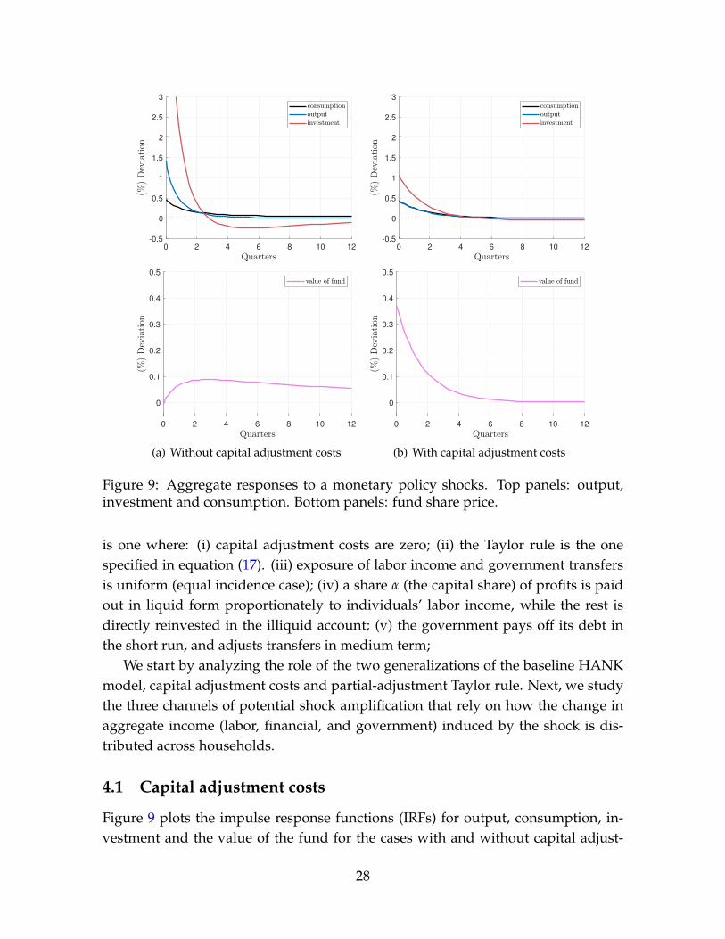
Figure 9: Aggregate responses to a monetary policy shocks. Top panels: output,investment and consumption. Bottom panels: fund share price.

is one where: (i) capital adjustment costs are zero; (ii) the Taylor rule is the onespecified in equation (17). (iii) exposure of labor income and government transfersis uniform (equal incidence case); (iv) a share α (the capital share) of profits is paidout in liquid form proportionately to individuals’ labor income, while the rest isdirectly reinvested in the illiquid account; (v) the government pays off its debt inthe short run, and adjusts transfers in medium term;

We start by analyzing the role of the two generalizations of the baseline HANKmodel, capital adjustment costs and partial-adjustment Taylor rule. Next, we studythe three channels of potential shock amplification that rely on how the change inaggregate income (labor, financial, and government) induced by the shock is dis-tributed across households.

4.1 Capital adjustment costs

Figure 9 plots the impulse response functions (IRFs) for output, consumption, in-vestment and the value of the fund for the cases with and without capital adjust-

28

ment costs. In the absence of adjustment costs, aggregate investment and outputreact strongly to the shock, but the share price of the fund barely moves: if any-thing, it falls slightly at impact because the profits of the intermediaries decrease atimpact.36

In the presence of adjustment costs, the investment response is much weaker,but there is a strong positive reaction in the value of the fund. This result highlightsan important shortcoming of this first generation of HANK models: in the data bothinvestment and asset prices react strongly after a monetary shock, but in the modellarge movements in prices can only be achieved with small changes in quantities,and viceversa. In contrast to the behavior of investment and output, aggregate con-sumption is largely unaffected by the presence of adjustment costs.

Figure 10 decomposes the IRF for aggregate consumption into direct and indirecteffects, following Kaplan, Moll, and Violante (2018). Direct and indirect effects arecomputed by counterfactuals. To compute the direct impact of a monetary shock,we let the real liquid rate change as in the baseline, but freeze all other prices andgovernment transfers at their steady-state value. Indirect effects are computed in asimilar way, varying one price at a time. The figure splits indirect effects betweenthe impact on consumption caused by the change in disposable labor income andthe change in the equity value.

As in Kaplan, Moll, and Violante (2018), we find in both scenarios that the in-direct general equilibrium channel accounts for about half of the total increase inaggregate consumption at impact. After a year, indirect effects account virtually forall of the consumption response. This stands in stark contrast with the representa-tive agent version of the New Keynesian model—where intertemporal substitutiondominates the transmission mechanism at all frequencies.

Even though the decomposition between direct and indirect channels is similarin the two cases, the relative importance of labor income versus equity prices inthe overall indirect effect changes with the introduction of the adjustment costs. Tounderstand why, notice that the initial impulse to aggregate demand always comesfrom the direct channel, i.e. the effect of the real rate cut on the consumption ofnon hand-to-mouth households and on the investment decisions made by the fund.This initial aggregate demand response pushes up employment and labor income,to which the consumption of hand-to-mouth households strongly responds, leadingto a second round of demand, employment and income expansion. This demand toincome feedback, which eventually reaches its equilibrium, is the main driver of

36The aggregate investment response in the case without adjustment cost is around 7% in thefirst quarter. We chose a smaller value for the upper limit of the vertical axis to better compare theconsumption and output response.

29

0 2 4 6 8 10 12

-0.1

0

0.1

0.2

0.3

0.4

0.5

0.6


0 2 4 6 8 10 12

-0.1

0

0.1

0.2

0.3

0.4

0.5

0.6


Figure 10: Decomposition of the consumption IRF to a monetary shock into directand indirect components.

consumption response in the case without adjustment costs.In the presence of adjustment costs, the investment response to the real rate

change is milder, which reduces the power of the aggregate demand channel. How-ever, there is now another channel contributing to aggregate consumption response:equity prices rise in response to the decrease in the real rate, a change that house-holds also react to by increasing their consumption (recall our comment on the MPCout of illiquid wealth in Figure 8). This extra consumption coming from the behav-ior of equity prices offsets the smaller expansion of labor income, explaining whyaggregate consumption moves by similar amounts in the two economies.

There is one important consequence of this different transmission mechanism.The identities of those households who gain from the expansion in asset prices arenot the same of those who benefit from the raise in employment and labor income.Figure 11 illustrates this distributional impact by showing the consumption reac-tion across the percentiles of the liquid asset. Without capital adjustment costs, poorhouseholds increase their consumption the most as labor income, the major driverof aggregate dynamics, plays a larger role on their response. With high capital ad-justment costs the overall consumption response is almost flat across the distribu-tion because wealthier households now benefit disproportionately more from thecapital gains.

30

0 10 20 30 40 50 60 70 80 90 100-0.2

0

0.2

0.4

0.6

0.8


0 10 20 30 40 50 60 70 80 90 100-0.2

0

0.2

0.4

0.6

0.8


Figure 11: Decomposition of the impact effect of a monetary shock on consumptionacross the distribution of liquid wealth. With and without capital adjustment costs.

4.2 Taylor rule

Figure 12 plots the IRFs to a monetary shock in the baseline and partial-adjustmentTaylor rule. Given our calibration, the partial-adjustment rule has only a minor im-pact on the equilibrium path of the nominal and real rate (see bottom panels). Asa consequence of that, aggregate quantities respond similarly in both cases (see up-per panels). In contrast to the effects of capital adjustment costs, the decompositionbetween direct and indirect effects is also unaffected, as seen in Figure 13.

4.3 Unequal income incidence

Figure 14 plots the impulse response of aggregate consumption under the differentparameterizations for the labor incidence function Γn presented in Figure 7.

The model with the “CPS (log)” unequal incidence generates only a tiny amountof amplification relative to the equal incidence case. The estimated incidence in-creases the cumulative aggregate consumption response over the first quarter from0.35% to 0.36%.37 Under the more extreme “CPS (asinh)” estimate, however, we findstronger amplification, with first quarter aggregate consumption rising from 0.35%to 0.43%.

Perhaps surprisingly, the SSA calibration of the incidence function yields a smalldampening relative to the equal incidence case. To understand why, recall that theSSA incidence function is U-shaped, meaning that incomes at both the bottom andthe top of the distribution are more exposed to fluctuations in aggregate incomesthan those in the middle. There are therefore two offsetting forces at work. More ex-

37The impulse response functions in the figure are the continuous time ones. To obtain the averageof the first quarter it is enough to integrate that impulse response in the figure from t = 0 to t = 1.

31

0 2 4 6 8 10 12

-0.5

0

0.5

1

1.5

2

2.5

3

0 2 4 6 8 10 12

-0.5

0

0.5

1

1.5

2

2.5

3

0 2 4 6 8 10 12

-1

-0.5

0

0.5

(a) Baseline Taylor rule

0 2 4 6 8 10 12

-1

-0.5

0

0.5

(b) Partial-adjustment Taylor rule

Figure 12: Aggregate responses to a monetary policy shock. Top panels: output,investment and consumption. Bottom panels: nominal, inflation and real rate.

posure at the bottom, where MPCs are higher than average, leads to amplification;but more exposure at the top, where MPCs are lower than average, leads to damp-ening. Furthermore, recall from Section 2.1 that it is the income-weighted covariancebetween MPCs and the elasticities, ˜COVi (MPCi, γi), that matters for amplification.Since individuals at the top of the distribution receive a higher share of aggregate in-come, the upward-sloping part of the SSA incidence function receives higher weightthan the downward-sloping part. The net effect is that the SSA incidence functionyields a slightly smaller consumption response than our baseline with equal inci-dence.

How does this magnitude of amplification compares with the work by Patterson(2018)? Patterson expresses her main amplification result in terms of the consump-tion multiplier: her estimated unequal income incidence function increases the gen-eral equilibrium multiplier from 1.3 to 1.42 (see her Table 3). She reports this as a40% increase in the net multiplier (from 0.3 to 0.42). In contrast, we measure am-plification in terms of the overall consumption response. Applying this metric to

32

0 2 4 6 8 10 12

-0.1

0

0.1

0.2

0.3

0.4

0.5

0.6

(a) Baseline rule

0 2 4 6 8 10 12

-0.1

0

0.1

0.2

0.3

0.4

0.5

0.6

(b) Partial-adjustment rule

Figure 13: Decomposition of the consumption IRF to a monetary shock into directand indirect components under different Taylor rules.

Patterson’s findings, the unequal distribution of labor income leads to a consump-tion response that is 1.42/1.3 times larger, which corresponds to a 9% increase, andhence in line with our findings.38

Our empirical analysis in Section 2.2 highlighted that government transfers arealso unequally distributed over the cycle. In the right panel of Figure 14 we comparethe consumption response for our baseline of equal incidence of government trans-fers with the one approximated from our CPS estimates. For transfers, the impact ofunequal incidence on the aggregate consumption response is even smaller than forlabor income. 39

4.4 Profit distribution

Our next candidate for the amplification of monetary shocks is the distribution ofprofits outside of steady state. Recall that our baseline distribution rule (24) assumesthat a fraction 1− α of profits is paid out to the liquid account proportionately to in-

38Formally, returning to simple model of Section 2.1, the total effect of a monetary shock on ag-gregate consumption can be written as dC = ˜MPCdY + ˜COVdY + Ddr, where the first two termsrepresent the general equilibrium component and Ddr represents the direct effect of the shock atimpact. Using the equilibrium condition C = Y, it is immediate that the total effect can be writtenas dC/dr = 1/(1− ˜MPC− ˜COV)D. In Patterson (2018), the GE multiplier with equal incidence(with ˜COV = 0) is estimated to be 1.3 and with unequal incidence 1.42. Therefore, adding unequalincidence amplifies the rise of C at impact by (1.42− 1.3)/1.3× 100 percent, i.e. 9 percent.

39We have experimented with alternative specifications for the transfer incidence function as well.For example, we have assumed that deviations of transfers from steady state are distributed equally(rather than proportionately to steady state transfers) across the entire population. This assumptionleads to a slight dampening compared to the “equal incidence" case.

33

0 2 4 6 8 10 12

-0.1

0

0.1

0.2

0.3

0.4

0.5

0.6

(a) Labor earnings

0 2 4 6 8 10 12

-0.1

0

0.1

0.2

0.3

0.4

0.5

0.6

(b) Government transfer

Figure 14: Consumption response to monetary shock in the model with unequalincidence of income across the household distribution.

dividuals’ labor income zitζit. We now let profit distributions into the liquid accountbe given by

Γπ(zt, ζt, Πt) = ztζt [(1− α)Π + (1−ω)(Πt − Π)] ,

where Π denotes steady-state monopoly profits and (1−ω) denotes the deviationsof profits from steady state that are paid out as liquid dividends instead of flowingto the investment fund.

We consider three different scenarios corresponding to three different values ofω. Our baseline model corresponds to the case ω = α so the same rule holds bothin and out of steady state. Second, we consider the case ω = 0 meaning that alldeviations from steady state profit are paid out in liquid form proportionately toearnings. Third, we set ω = 1 meaning that all deviations from steady state profitsend up in the illiquid account and are distributed to individuals according to theirholdings of shares in the investment fund.

Figure 15 summarizes the results for the economy without capital adjustmentcosts. The left panel shows the consumption response for the three alternative profitdistribution rules based on the different values for ω. When a large share of profitsis paid into the liquid account (low ω), the fall in profits after an expansionary mon-etary shock directly depresses household disposable income. When it is, instead,retained into the illiquid account (high ω), it drags down investment (right panel)which, in turn, lowers demand for labor and therefore also curtails the expansion ofhousehold disposable income. In our experiments it is the second of these two off-setting forces that dominates: aggregate consumption increases more when profits

34

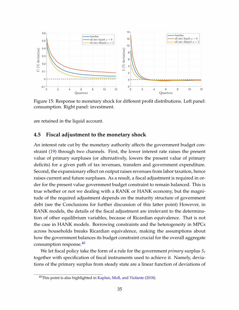
0 2 4 6 8 10 12

-0.1

0

0.1

0.2

0.3

0.4

0.5

0.6

0 2 4 6 8 10 12

-2

0

2

4

6

8

10

12

14

Figure 15: Response to monetary shock for different profit distributions. Left panel:consumption. Right panel: investment.

are retained in the liquid account.

4.5 Fiscal adjustment to the monetary shock

An interest rate cut by the monetary authority affects the government budget con-straint (19) through two channels. First, the lower interest rate raises the presentvalue of primary surpluses (or alternatively, lowers the present value of primarydeficits) for a given path of tax revenues, transfers and government expenditure.Second, the expansionary effect on output raises revenues from labor taxation, henceraises current and future surpluses. As a result, a fiscal adjustment is required in or-der for the present value government budget constraint to remain balanced. This istrue whether or not we dealing with a RANK or HANK economy, but the magni-tude of the required adjustment depends on the maturity structure of governmentdebt (see the Conclusions for further discussion of this latter point) However, inRANK models, the details of the fiscal adjustment are irrelevant to the determina-tion of other equilibrium variables, because of Ricardian equivalence. That is notthe case in HANK models. Borrowing constraints and the heterogeneity in MPCsacross households breaks Ricardian equivalence, making the assumptions abouthow the government balances its budget constraint crucial for the overall aggregateconsumption response.40

We let fiscal policy take the form of a rule for the government primary surplus St

together with specification of fiscal instruments used to achieve it. Namely, devia-tions of the primary surplus from steady state are a linear function of deviations of

40This point is also highlighted in Kaplan, Moll, and Violante (2018).

35

interest payments on debt rbt Bg

t − rbBg, of aggregate labor income wtNt − wN, andof the level of debt Bg

t − Bg itself:

St = S− (1− ρR)(rbt Bg

t − rbBg) + ρN(wtNt − wN)− ρB(Bgt − Bg) (25)

where parameters (ρR, ρN, ρB) control the primary surplus sensitivity to these devi-ations.41 Substituting the fiscal rule (25) into the government budget constraint (19),the implied evolution of government assets can be written as

Bgt = ρR(rb

t Bgt − rbBg) + ρN(wtNt − wN)− ρB(Bg

t − Bg) . (26)

To understand the implications of different fiscal rules for the evolution of gov-ernment debt, consider the following two extreme cases: (ρR = ρN = 0) and(ρR = 1, ρN = τ). When (ρR = ρN = 0), government debt is kept fixed at its steadystate value independently of changes in revenue and borrowing costs. Thus, the pri-mary surplus matches the interest payments on debt at all times (i.e., St = −rtBt).When (ρR = 1, ρN = τ), the (initial) primary surplus varies proportionally withgovernment tax revenues and government debt adjusts to accommodate the overallsurplus.42

While (25) defines the response of the primary surplus to changes in the govern-ment budget, it does not pin down the way in which the surplus is achieved. Thereare numerous alternatives here: the same surplus can be obtained by either appro-priately adjusting one of the instruments (Tt, τt and Gt), or any combination of them.In our baseline we have assumed that: (i) government debt absorbs all of the short-run fiscal imbalance (ρR = 1, ρN = τ) and (ii) transfers Tt adjust in the medium termto bring the debt back to steady-state, while government expenditures and labor tax

41See Leith and Leeper (2016) for a similar formulation.42We assume that ρB > ρR rb so that the future surpluses response to movements in real debt guar-

antees limt→∞ Bgt = Bg for arbitrary deviations of debt from steady state. To see how this condition

is sufficient to guarantee a converging debt path, note that we can rewrite (26) as

Bgt = ρR(rb

t Bgt − rb Bg) + ρS(wtNt − wN)− ρB(Bg

t − Bg)

Bgt = (ρRrb

t − ρB)(Bgt − Bg) + ρR Bg(rb

t − rb) + ρS(wtNt − wN).

If we restrict attention to sequences {rbt , Nt, wt} that converge back to their steady state as t → ∞,

then the dynamics of real debt for sufficiently large t are

Bgt = (ρR rb − ρB)(Bg

t − Bg),

which imply that Bgt → Bg if ρB > ρR rb.

36

0 2 4 6 8 10 12

0

0.2

0.4

0.6

0.8

1

0 2 4 6 8 10 12

-60

-40

-20

0

20

40

60

80

Figure 16: Consumption and surplus response to monetary shock under three dif-ferent types of fiscal adjustments: (i) ρR = 1, ρN = τ: government debt respondsto changes in interest payments as well as to changes in tax revenue (the baseline);(ii) ρR = 1, ρN = 0: government debt responds to changes in interest payments, buttransfers compensate for changes in tax revenues; (iii) ρR = 0, ρN = 0: transfersadjust to keep government debt fixed. In all cases ρB = 0.05.

rate are kept fixed at their steady state values.43 In this section, we consider alterna-tives to this baseline that differ (i) in the values of the parameters ρR, ρN measuringthe reaction of primary surplus to deviations in government’s revenues and interestexpenses; and (ii) in the fiscal instrument used to adjust the surplus.

Figure 16 shows consumption and surplus for the first experiment. A fiscal rulethat keeps the value of outstanding debt constant (ρR = 0, ρN = 0) leads to a firstquarter consumption response twice as large as that of our baseline (ρR = 1, ρN = τ)

where government debt is used to smooth out the initial fluctuations. The corre-sponding surplus deviation is shown in the right panel. While the government in-

43To see the implications of the rule for the behavior of transfers in the case that the labor tax rateand government expenditures are fixed, note that we can write the surplus as

St = τwtNt − Tt − GSt = −(Tt − T) + (τwtNt − T − G)

St = −(Tt − T) + τ(wtNt − wN) + (τwN − T − G)

or in terms of transfer

Tt − T = −(St − S) + τ(wtNt − wN)

Tt − T = −(− (1− ρR)(rb

t Bgt − rb Bg) + ρN(wtNt − wN)− ρB(Bg

t − Bg))+ τ(wtNt − wN)

Tt − T = (1− ρR)(rbt Bg

t − rb Bg) + (τ − ρN)(wtNt − wN) + ρB(Bgt − Bg).

So in the baseline (ρR = 1, ρN = τ), transfers increase only when debt deviates from steady state.

37

0 2 4 6 8 10 12

0

0.2

0.4

0.6

0.8

1

0 2 4 6 8 10 12

0

0.5

1

1.5

2

2.5

3

3.5

Figure 17: Consumption and output response when different instruments are usedto achieve the desired fiscal surplus.

creases its primary surplus in the baseline by saving the extra tax revenue τ(wtNt −wN), the fixed debt case has the government running down its surplus as it in-creases transfers to households in the amount of −(rb

t Bgt − rbBg) + τ(wtNt − wN).

The intuition is simple: households’ disposable income rises with the increase intransfers and generates an additional impulse to aggregate consumption. We alsoexplore the impact of an intermediate policy (ρR = 1, ρN = 0) that keeps primarysurplus constant at impact. In this case, the government adjusts transfers in propor-tion to the rising revenues, but uses the lower borrowing cost to pay off its debt.44

The aggregate consumption response under this alternative rule is between the twoprevious cases, as one should expect.

In Figure 17, we compare the fiscal instrument that is used to adjust primarysurpluses. We concentrate on the case with debt fixed (ρR = 0, ρN = 0) and ex-periment with different alternative fiscal instruments to deliver the desired surplus.We compare three alternatives: we adjust transfers Tt only, the labor tax τt only, orgovernment expenditures Gt only. Among these different instruments, using trans-fers to adjust the government budget leads to the largest aggregate consumptionresponse, while changing government expenditures promotes the largest increasein output. Transfers directly affect household disposable income, and because of itslump-sum nature, this bump in income is especially potent for low-income hand-to-mouth households. Adjusting government expenditures leads to a one-to-one

44In this case the behavior of transfers is given by

Tt − T = τ(wtNt − wN) + ρB(Bgt − Bg).

38

ExperimentHANK HANK HANK

capital adj. cost partial adj. Taylor

Baseline 1.000 1.000 1.000

- (1.000) (0.991) (0.941)

Unequal labor incidenceCPS (asinh) 1.234 1.188 1.232

CPS (log) 1.024 1.010 1.023

SSA 0.934 0.973 0.937

Profit distributionProfit all liq. 1.199 1.089 1.066

Profit all illiq. 0.904 0.943 0.931

Fiscal reactionρR = 1, ρN = 0 1.573 1.265 1.571

ρR = 0, ρN = 0 - - -

(Transfers adjust) 2.140 1.819 2.358

(Labor tax adjusts) 1.593 1.436 1.773

(Government exp. adjust) 1.538 1.379 1.751

Table 3: First quarter aggregate consumption response to monetary shock relativeto the baseline.Values in each column are normalized by the consumption in the first row of the correspondingcolumn (baselines). Values in brackets in the second row denote the relative consumption of thebaseline specification relative to the baseline in HANK without capital adjustment costs and withthe standard Taylor rule (first column, first row). See Section 4.3 for a description of the unequallabor incidence exercises, Section 4.4 for profit distribution, and Section 4.5 for fiscal adjustment.

impact on aggregate demand, but some crowding out in private consumption. Cut-ting the labor tax distributes resources to households proportionally to their laborincome. This force tends to primarily benefit high-income low-MPC individuals,which explains why consumption goes up by less in this scenario.

To sum up, the different assumptions about timing of the fiscal response ex-plored in Figure 16 and instrument choice explored in Figure 17 generate substantialdifferences in the aggregate consumption response. In the Conclusions, we discusswhy these results on the sensitivity of monetary policy to the fiscal reaction are nota consequence of restricting the government to only issue short-term debt.

39

4.6 Summary

Table 3 summarizes our different experiments. The first column (HANK) refers tothe baseline model specification. The other columns report results for the modelswith aggregate capital adjustment costs and a more sophisticated Taylor rule. Thevalues in the table denote the difference in first quarter consumption following anexpansionary monetary shock, relative to the baseline from the same column.

The presence of adjustment cost lessens the impact of all the elements we haveconsidered. This can be traced to the smaller impact of the shock on investment,which curtails the aggregate demand response. As a result, all channels that rely onthe general equilibrium feedback are weakened. Results under the partial-adjustmentrule are much closer to the baseline, except for the profit distribution exercises thatare dampened under the different rule. Quantitatively, however, the main takeawayis about the importance of the fiscal response relative to other elements considered:its impact on aggregate consumption response is much larger than that of unequalincome incidence or the distribution of profits. 45

5 Conclusions

Heterogeneous Agent New Keynesian (HANK) models contain several channelsthat amplify or dampen the response of aggregate consumption to a monetary pol-icy shock which are either absent or less relevant in Representative Agent New Key-nesian (RANK) models. Our goal in this paper has been to provide some guidanceon how a subset of these channels compare in terms of their quantitative strength.We performed these exercises in a rich two-asset HANK model calibrated to be con-sistent with micro evidence on household earnings, wealth distributions, and MPCs.

The model elements that we have considered include: unequal incidence of fluc-tuations in aggregate labor income, capital income, and government transfers acrosshouseholds; capital adjustment costs; and different rules for fiscal and monetarypolicy. Our findings suggest that of these elements, assumptions about how thegovernment budget constraint adjusts in response to the monetary shock is by farthe most important.

In our model, all government debt and household liquid assets are of infinitelyshort duration with an instantaneously adjusting interest rate. In reality, however,a substantial fraction of government debt and household assets are long-term, withcoupon rates that were set in the past and that do not adjust to changes in short rates.

45Check the Online Appendix for an equivalent of Table 3 for the representative agent counterpartof our model, together with a discussion.

40

In HANK models, these assumptions about the maturity structure of governmentdebt are not innocuous.

The extent to which a change in the path of interest rates affects the intertem-poral government budget constraint depends on the difference between the dura-tion of the government’s assets and its liabilities. The governments’ only asset isits claim on future primary surpluses which, in the absence of general equilibriumeffects, delivers a fixed constant stream of resources. The government could thusperfectly hedge its exposure to interest rate changes by issuing a constant couponperpetual bond, in which case monetary policy would not require any fiscal adjust-ment (although general equilibrium effects that alter primary surpluses would stillnecessitate a fiscal adjustment).

There is thus a sense in which our assumption of infinitely short duration debtleaves the government maximally exposed to monetary policy, and thus requires thelargest fiscal adjustment among alternative possible assumptions about the maturitystructure of government debt. In RANK models, none of this matters, because ofRicardian Equivalence. But in HANK models, where Ricardian Equivalence fails,a shorter maturity structure translates into a larger required fiscal adjustment andhence a wider set of possible indirect effects of the monetary shock.

We leave the systematic analysis of the effects of monetary policy with long-termgovernment debt in HANK for future research – see Auclert, Rognlie, and Straub(2020) for a recent example. We note that while increasing the duration of gov-ernment debt may mitigate the effects of fiscal policy for monetary transmission inHANK, it introduces additional effects of monetary policy that are absent in RANKand in HANK models with short-term debt. This is because even though the gov-ernment is better hedged against interest rate changes with longer-term debt, thehouseholds who hold the other side of these claims as long-duration assets are nowmore exposed to changes in interest rates. This introduces additional redistributiveeffects of monetary policy.

Consistent with previous findings from simpler, analytic HANK models, we findthat unequal incidence of labor income, profit income and transfers can all eitheramplify or dampen the effect of a monetary shock. For incidence functions impliedby our estimates from US data, the degree of amplification or dampening is rel-atively small. With respect to this finding, the main caveat is that our estimatedincidence functions are not conditional on a monetary shock. An interesting avenueof research is the analysis of whether heterogeneous exposure across householdsvaries with respect to the shock and how this affect the propagation of the mainaggregate shocks that account for US fluctuations. See Broer, Kramer, and Mitman

41

(2020) for recent progress on this question.With respect to the distribution of capital income across households, we em-

phasized that whether profits end up in liquid or illiquid accounts is important forthe dynamics of investment. In our model, investment is financed by inflows intoilliquid assets (equity, housing) whereas liquid assets are instead invested in gov-ernment bonds. In a more general model in which households deposit their liquidwealth in the banking sector and banks intermediate funds to firms, this distinc-tion may be less sharp, depending on the transaction cost faced by banks vis-à-visindividuals.

Finally, we emphasized that capital adjustment costs modify the transmissionmechanism by muting movements in the quantities of capital and amplifying move-ments in equity prices. While this feature of the model improves the macro-financeside of the model relative to e.g. Kaplan, Moll, and Violante (2018), its predictions re-main very far from the basic asset pricing facts documented in the literature. Goingforward, this is another dimension where progress should be made. Recent workby Lenel and Kekre (2019) is an important step in this direction.

42

References

ACHARYA, S., AND K. DOGRA (2018): “Understanding HANK: Insights from a PRANK,”Staff Reports 835, Federal Reserve Bank of New York.

AUCLERT, A. (2019): “Monetary policy and the redistribution channel,” American EconomicReview, 109(6), 2333–67.

AUCLERT, A., AND M. ROGNLIE (2018): “Inequality and Aggregate Demand,” NBER Work-ing Papers 24280, National Bureau of Economic Research, Inc.

AUCLERT, A., M. ROGNLIE, AND L. STRAUB (2020): “Micro Jumps, Macro Humps: Mone-tary Policy and Business Cycles in an Estimated HANK Model,” NBER Working Papersw26647, National Bureau of Economic Research, Inc.

BAYER, C., R. LUETTICKE, L. PHAM-DAO, AND V. TJADEN (2019): “Precautionary Savings,Illiquid Assets, and the Aggregate Consequences of Shocks to Household Income Risk,”Econometrica, 87(1), 255–290.

BELLEMARE, M., AND C. WICHMAN (2018): “Elasticities and the Inverse Hyperbolic SineTransformation,” University of Minnesota.

BERGER, D., L. BOCOLA, AND A. DOVIS (2019): “Imperfect Risk-Sharing and the BusinessCycle,” Discussion paper, Stanford University.

BERNSTEIN, J. (2019): “Redistribution and the Asymmetric Transmission of AggregateShocks,” Discussion paper, Princeton University.

BILBIIE, F. (2017): “The New Keynesian Cross: Understanding Monetary Policy with Hand-to-Mouth Households,” Discussion paper, Center for Economic Policy Research.

BILBIIE, F. O., D. R. KÄNZIG, AND P. SURICO (2019): “Capital, Income Inequality, and Con-sumption: The Missing Link,” Discussion paper, CEPR Discussion Paper No. DP14118.

BROER, T., N.-J. HARBO HANSEN, P. KRUSELL, AND E. OBERG (2016): “The New Key-nesian Transmission Mechanism: A Heterogenous-Agent Perspective,” CEPR DiscussionPapers 11382, C.E.P.R. Discussion Papers.

BROER, T., J. KRAMER, AND K. MITMAN (2020): “The Curious Incidence of Shocks Alongthe Income Distribution,” Discussion paper, IIES, Stockholm.

CHRISTIANO, L. J., M. S. EICHENBAUM, AND M. TRABANDT (2016): “Unemployment andBusiness Cycles,” Econometrica, 84(4), 1523–1569.

COCHRANE, J. H. (2017): “The New-Keynesian Liquidity Trap,” Journal of Monetary Eco-nomics, 92, 43.

CUI, W., AND V. STERK (2019): “Quantitative Easing,” Discussion paper, UCL.DEBORTOLI, D., AND J. GALI (2018): “Monetary Policy with Heterogeneous Agents: In-

sights from Tank Models,” Working paper, CREI.DEN HAAN, W., P. RENDAHL, AND M. RIEGLER (2015): “Unemployment (Fears) and De-

flationary Spirals,” Discussion paper, Centre for Macroeconomics (CFM).GORNEMANN, N., K. KUESTER, AND M. NAKAJIMA (2014): “Doves for the Rich, Hawks for

the Poor? Distributional Consequences of Monetary Policy,” Discussion paper, FederalReserve Bank of Philadelphia.

GUERRIERI, V., AND G. LORENZONI (2011): “Credit Crises, Precautionary Savings, and theLiquidity Trap,” NBER Working Papers 17583, National Bureau of Economic Research.

43

GUVENEN, F., F. KARAHAN, S. OZKAN, AND J. SONG (2015): “What Do Data on Millionsof U.S. Workers Reveal about Life-Cycle Earnings Risk?,” NBER Working Papers 20913,National Bureau of Economic Research.

GUVENEN, F., S. SCHULHOFER-WOHL, J. SONG, AND M. YOGO (2017): “Worker Betas: FiveFacts About Systematic Earnings Risk,” American Economic Review, 107(5), 98–403.

HEATHCOTE, J., F. PERRI, AND G. L. VIOLANTE (2020): “The Rise in Earnings Inequality:Does the Cycle Drive the Trend?,” Discussion paper, Princeton University.

KAPLAN, G., B. MOLL, AND G. L. VIOLANTE (2018): “Monetary Policy According toHANK,” American Economic Review, 108(3), 697–743.

KAPLAN, G., AND G. L. VIOLANTE (2014): “A Model of the Consumption Response toFiscal Stimulus Payments,” Econometrica, 82(4), 1199–1239.

KAPLAN, G., G. L. VIOLANTE, AND J. WEIDNER (2014): “The Wealthy Hand-to-Mouth,”Brookings Papers on Economic Activity, 48(1 (Spring), 77–153.

KEKRE, R. (2019): “Unemployment Insurance in Macroeconomic Stabilization,” Discussionpaper, Booth School of Business, University of Chicago.

LEITH, C., AND E. LEEPER (2016): “Understanding Inflation as a Joint Monetary - Fiscal Phe-nomenon,” Working Papers 2016-01, Business School - Economics, University of Glasgow.

LENEL, M., AND R. KEKRE (2019): “Redistribution, Risk Premia, and the Macroeconomy,”Discussion paper, Princeton University.

LUETTICKE, R. (2015): “Transmission of Monetary Policy and Heterogeneity in HouseholdPortfolios,” Discussion paper, University of Bonn.

MCKAY, A., E. NAKAMURA, AND J. STEINSSON (2016): “The Power of Forward GuidanceRevisited,” American Economic Review, 106(10), 3133–58.

MCKAY, A., AND R. REIS (2016): “The Role of Automatic Stabilizers in the U.S. BusinessCycle,” Econometrica, 84, 141–194.

OH, H., AND R. REIS (2012): “Targeted Transfers and the Fiscal Response to the Great Re-cession,” Journal of Monetary Economics, 59(S), S50–S64.

PATTERSON, C. (2018): “The Matching Multiplier and the Amplification of Recessions,”Discussion paper, MIT.

RAVN, M. O., AND V. STERK (2017): “Job Uncertainty and Deep Recessions,” Journal ofMonetary Economics, 90, 125–141.

ROTEMBERG, J. J. (1982): “Sticky Prices in the United States,” Journal of Political Economy,90(6), 1187–1211.

SIMS (2004): “The Inflation-Targeting Debate,” Discussion paper, Princeton University.SIMS, C. A. (1980): “Macroeconomics and Reality,” Econometrica, 48(1), 1–48.WERNING, I. (2015): “Incomplete Markets and Aggregate Demand,” Working Paper 21448,

National Bureau of Economic Research.

44

a further look at the propagation of monetary policy

Documents