a functional coefficient model view of the feldstein–horioka puzzle

Journal of International Money and Finance 29 (2010) 37–54

Contents lists available at ScienceDirect

Journal of International Moneyand Finance

journal homepage: www.elsevier .com/locate/ j imf

A functional coefficient model view of theFeldstein–Horioka puzzle

H. Herwartz a, F. Xu a,b,*

a Institute for Statistics and Econometrics, Christian-Albrechts-University of Kiel, Olshausenstr. 40-60, 24118 Kiel, Germanyb European University Institute, Villa La Fonte, Via Delle Fontanelle 10, 50014 San Domenico di Fiesole (FI), Italy

JEL classification:C14C23E21E22

Keywords:Saving–investment relationFeldstein–Horioka puzzleFunctional coefficient models

* Corresponding author. Tel.: þ39 0554685607;E-mail addresses: [email protected]

1 For a detailed review over the literature on th

0261-5606/$ – see front matter � 2008 Elsevier Ldoi:10.1016/j.jimonfin.2008.12.001

a b s t r a c t

What does the saving–investment (SI) relation really measure andhow should the SI relation be measured? These are two of themost discussed issues triggered by the so-called Feldstein–Horiokapuzzle. Based on panel data we introduce a new variant of func-tional coefficient models that allows to separate long and short tomedium run parameter dependence. The new modeling frame-work is applied to uncover the determinants of the SI relation.Macroeconomic state variables such as openness, the age depen-dency ratio, government current and consumption expendituresare found to affect the SI relation significantly in the long run.

� 2008 Elsevier Ltd. All rights reserved.

1. Introduction

‘‘How internationally mobile is the world’s supply of capital?’’ This is the question investigated byFeldstein and Horioka (1980), henceforth FH (1980). By means of a between regression for OECDcountries, FH (1980) document a strong correlation linking domestic investment and saving, which isargued to be at odds with capital mobility. Following FH (1980) one would expect that under perfectcapital mobility the correlation between a country’s saving and investment ratio should be small. Assuch the diagnosed high correlation is in contrast to established theoretical frameworks in openeconomy macroeconomics and also to the belief that capital markets have experienced substantialliberalization.

The so-called ‘‘Feldstein–Horioka puzzle’’ (FH puzzle) has provoked a lively discussion in boththeoretical and empirical literature.1 Two of the most investigated questions are: what does the

fax: þ39 0554685804.l.de (H. Herwartz), [email protected], [email protected] (F. Xu).e FH puzzle the reader may consult Coakley et al. (1998).

td. All rights reserved.

mailto:[email protected]



www.sciencedirect.com/science/journal/02615606

www.elsevier.com/locate/jimf

H. Herwartz, F. Xu / Journal of International Money and Finance 29 (2010) 37–5438

saving–investment relation really measure and how should the saving–investment relation bemeasured? To answer the first question, various determinants of the SI relation have been suggestedin the theoretical literature such as population growth (Obstfeld, 1986), the intertemporal budgetconstraint (Coakley et al., 1996; Taylor, 2002), output fluctuations in non-traded goods (Tesar, 1993),or current account (CA) targeting (Artis and Bayoumi, 1992). Since the intertemporal budgetconstraint seems to be one of the most convincing reasons for a high SI relation, most recentempirical investigations of the SI relation concentrate on a potential cointegration relation betweensaving and investment.2 Thereby, error correction models are suggested as the suitable framework tomeasure the SI relation.3 However, no unique evidence for a cointegration relation between savingand investment is found. Compared to the abundant empirical investigations for the intertemporalbudget constraint, empirical contributions linking all other determinants of the SI relation are ratherscarce. A few exceptions (and identified factors) are Summers (1988) (government budget balance),AmirKhalkhali et al. (2003) (government size), Kasuga (2004) (financial structures), Sachsida andCaetano (2000) (the variability between external and domestic saving) and Herwartz and Xu (2008a)(bounds on current account measures induced by policy controls or financial crises). Furthermore, inthese contributions there exists no unique model to measure the SI relation along with potentialdeterminants.

In this paper, we suggest a new semiparametric approach to investigate the determinants of the SIrelation. It is derived as a bivariate generalization of functional coefficient models (Cai et al., 2000). Weadopt a new bootstrap based venue of inference which is suitably immunized against adverse effects of(mild) under- or oversmoothing of semiparametric functional estimates. To identify potential deter-minants of the SI relation, the formalized semiparametric model copes with cross-sectional hetero-geneity, time and factor dependence. It allows to separate deterministic from measurable economicconditions characterizing the empirical SI relation over time. Moreover, long and short run factorimpacts on the SI relation can be distinguished.

We analyse annual data spanning the period 1971–2002 for various (partly overlapping) cross-sections characterizing the world economy, developing countries, the OECD, the EU and the Euro area.With respect to the choice of potential factor variables we rely on recent studies by Edwards (1995),Debelle and Faruqee (1996), Milesi-Ferretti and Razin (1997, 1998), Masson et al. (1998), and Chinn andPrasad (2003). The employed factor variables allow a classification into three groups: potentialdeterminants of saving, investment or the current account balance and factors describing the inte-gration of goods and financial markets. In addition, the scope of variables measuring the dependence ofthe SI relation on country size is addressed.

From functional coefficient models, an economy’s degree of openness, its age dependency ratio andgovernment current and consumption expenditures are identified to have a significantly negativeinfluence on the SI relation in the long run. Besides, countries with high GDP (measuring the effect ofcountry size) are more likely to have a high SI relation. As a consequence, empirically high SI relationscould reflect goods market frictions, demographic development or fiscal consolidation rather thanbeing puzzling. This paper provides firsthand evidence to support particular theoretical views on the SIrelation.

The remainder of the paper is organized as follows. In the next section we initiate our empiricalanalysis by highlighting that the empirical SI relation has experienced some weakening over morerecent time periods. Given that the link between domestic saving and investment is likely heteroge-nous over time as well as country specific we introduce a semiparametric approach to evaluate the SIrelation in Section 3. Empirical results are provided in Section 4. Section 5 summarizes briefly our mainfindings and concludes. More detailed information on the investigated (cross-sections of) economiesand factors is given in the Appendices 1 and 2.

2 Abbott and Vita (2003), Gulley (1992), Haan and Siermann (1994), Ho (2002a,b), Leachman (1991), Lemmen and Eijffinger(1995), Miller (1988), Vita and Abbott (2002).

3 Bajo-Rubio (1998), Coiteux and Olivier (2000), Jansen (1996, 1998), Jansen and Schulze (1996), Moreno (1997), Ozmen andParmaksiz (2003a,b), Pelagidis and Mastroyiannis (2003); Pelgrin and Schich (2004), Schmidt (2001), Sinha and Sinha (2004),Taylor (1996, 1998).

H. Herwartz, F. Xu / Journal of International Money and Finance 29 (2010) 37–54 39

2. Preliminary analyses

In this section we firstly introduce the data and motivate the use of alternative cross-sections.Furthermore, stylized features of the empirical SI relation, as, e.g. its downward trending behavior, areillustrated by means of between regressions as in FH (1980).

We investigate the SI relation with seven alternative (partly overlapping) cross-sections usingannual data from 1971 to 2002 drawn from the World Development Indicators CD-Rom 2004 pub-lished by the World Bank. The first and most comprehensive sample covers 97 countries from all overthe world (W97), for which most observations of the saving and investment ratio from 1971 to 2002 areavailable. This sample is one of the largest cross-sections that has been considered to analyse the SIrelation. For six countries data for 2002 are not available. These missing values are estimated by meansof univariate autoregressive models of order 1 with intercept. A list of all 97 countries contained in W97is provided in the Appendix 2. All OECD countries except Czech Republic, Poland, Slovak Republic andLuxembourg comprise the second cross-section denoted with O26. The first three countries are notincluded due to data nonavailability. Luxembourg is often excluded in empirical analyses of the SIrelation since its large international banking sector has not been properly considered in nationalaccount data (Coiteux and Olivier, 2000; Jansen, 2000). The third sample we consider covers 14 majorcountries of the European Union (E14), which are the O26 economies without Australia, Canada,Hungary, Iceland, Japan, Korea, Mexico, New Zealand, Norway, Switzerland, Turkey and the US. Con-trasting this subgroup with O26 may reflect the EU effect on the SI relation. As the fourth cross-section11 Euro area economies excluding Luxembourg (E11) are investigated. E11 differs from E14 by exclusionof Denmark, Sweden and the UK. In the Euro area, there is no exchange rate risk and financial marketsshould be more integrated in comparison with the remainder of the EU. To offer a ‘complementary’view at the link between market integration and the SI relation, we investigate a fifth cross-section(O15) defined as O26 minus E11. Here we focus on weaker forms of market integration and try to isolatetheir impact on the SI relation. Conditioning the SI relation on the state of economic development hasbecome an important avenue to solve the FH puzzle. Therefore, a sixth cross-section collects lessdeveloped economies. It is obtained as W97 minus O26, Luxembourg, Hong Kong and Singapore,denoted with L68. Finally, to improve the comparability of our results with FH (1980) we consider thecross-section employed in their initial contribution (F16). This comprises 16 OECD countries namelyO26 excluding France, Hungary, Korea, Mexico, Norway, Portugal, Spain, Switzerland and Turkey.

The between regression adopted by FH (1980) is

I�i ¼ aþ bS�i þ ei; i ¼ 1;.N; (1)

where I�i ¼ 1=TPT

t¼1 I�it , S�i ¼ 1=TPT

t¼1 S�it , I�it ¼ Iit=Yit and S�it ¼ Sit=Yit , with Iit, Sit and Yit, t¼ 1,.,T,denoting gross domestic investment, gross domestic saving and gross domestic product (GDP) in timeperiod t and country i, respectively. In this study between regressions are thought to provide a firstview at the data. It can be argued that estimating the model in (1) suffers from joint endogeneity.Nevertheless, it has been often found that taking account of the endogeneity issue does not changeempirical results qualitatively, as can be seen in FH (1980). Another problem of applying betweenregressions may lie in the potential non-stationarity of saving and investment ratios. However,applying cross-sectional regressions delivers the same evidence of a time varying SI relation asreported below. Since the main purpose of this paper is to introduce the functional coefficient model toanalyse the SI relation, we address endogeneity and non-stationarity in Section 3.5 attentively.

Implementing the between regression in (1) with annual data covering the period 1971–2002, weobtain the results shown in panel A of Table 1. Between regression estimates are significantly positivein all cross-sections except E11 and E14. Excluding the two latter cross-sections from model compar-ison, between regressions offer degrees of explanation between 52% (L68, O26) and 83% (O15).Following the arguments in FH (1980) a significantly positive SI relation in W97 is not surprising. Somepatterns of capital market segmentation are likely over a group of 97 economies sampled from all overthe world. For E14 and E11, the coefficient estimates are insignificant and thereby confirm the EU andEuro effect. In F16, both the estimated SI relation (0.62) and the degree of explanation (0.58) are smallerfor the period 1971–2002 compared with the corresponding results (0.89 and 0.91) given in FH (1980)

Table 1Between regressiona; I�i ¼ aþ bS�i þ ei .

Samples W97 L68 O26 O15 F16 E14 E11

Panel A: 1971–2002bb 0.43 (11.24) 0.40 (8.47) 0.59 (5.11) 0.77 (7.96) 0.62 (4.44) 0.13 (0.53) �0.16 (�0.71)R2 0.57 0.52 0.52 0.83 0.58 0.02 0.05Norm 0.57 0.34 6.00 1.11 4.05 0.60 1.23Homosk 3.79 4.55 0.79 1.80 0.66 4.63 0.06

Panel B: 1971–1986bb 0.44 (9.44) 0.39 (7.13) 0.69 (6.58) 0.86 (10.43) 0.66 (4.50) 0.36 (1.46) 0.18 (0.78)R2 0.48 0.44 0.64 0.89 0.59 0.15 0.06

Panel C: 1987–2002bb 0.38 (9.96) 0.39 (7.80) 0.39 (3.27) 0.65 (5.23) 0.30 (2.24) �0.02 (�0.10) �0.14 (�0.90)R2 0.51 0.48 0.31 0.68 0.26 0.00 0.08

a This table reports slope estimates from the between regressions of the investment ratio on the saving ratio; t-statistics appearin parentheses next to the coefficient estimates. Coefficients which are significant at the 5% level are highlighted in bold face. Inaddition, lines with ‘norm’ and ‘homosk’ document Jarque–Bera and LM statistics testing normality and homoskedasticity,respectively. For the LM test the alternative hypothesis is the heterogenous error variance conditional on the squared averagesaving ratio. Test statistics that are in favor of the alternative hypothesis with 5% significance are highlighted in bold face.


for the period 1960–1974. This finding is consistent with the presumption that capital mobility hasincreased over time. Furthermore, it could be shown that the estimated SI relation becomes insignif-icant in F16 if Japan, the UK and the US are excluded, thereby signalling a large country effect. Diag-nostic statistics (Jarque–Bera test on normality and LM test on homoskedasticity) reveal that betweenresiduals mostly match typical assumptions to justify standard tests on parameter significance.

Given the weakened evidence in favor of a large or even significant SI relation conditional on morerecent samples in comparison with FH (1980), it is sensible to address the robustness of the previousresults by splitting the sample into sub-samples. Two equally sized sub-samples (1971–1986 and 1987–2002) are considered for this purpose. It can be seen from panels B and C of Table 1 that the estimatedSI relation has decreased in almost all cross-sections. This evidence is consistent with the generallyimproving integration of capital and goods markets. Between estimates are insignificantly differentfrom zero in E14 and E11 for both subperiods. Although the SI relation in OECD economies (O26, F16,O15) is still significantly different from zero, it is much smaller for the more recent period. The degreeof explanation achieved by between regressions for the second subset is lower than for the first, andvaries between 26% (F16) and 68% (O15) when E11 and E14 are excluded.

In the light of the previous results one may conjecture that the FH puzzle is not such a big puzzleanymore when concentrating on more recent time windows. In a similar vein, using data for 12 OECDcountries from 1980 to 2001, Coakley et al. (2004) show the insignificance of the SI relation by means ofnon-stationary panel models. Blanchard and Giavazzi (2002) also document a small SI relation ina pooled regression for the EU area using the sample period 1991–2001. From a statistical as well aseconomic viewpoint, however, potential time variation of the SI relation provokes some subsequentissues. With regard to statistical aspects it is not clear in how far conclusions offered by (misspecified)time homogenous econometric models are spurious or robust under respecification of the model. Froman economic perspective it is tempting to disentangle the economic forces behind the observeddecreasing trend in the SI relation. With regard to this aspect it is of particular interest to separatedeterministic time features from measurable economic factors driving the SI relation.

3. Functional coefficient models

The preceding analyses have shown that the link between domestic saving and investment exhibitssome downward trending behavior. Moreover, the SI relation is likely cross-section specific as arguedby Herwartz and Xu (2008b). Given the likelihood of parameter variation over two data dimensions, allempirical approaches followed so far carry the risk of providing biased results since at most onedimension of potential parameter dependence has been taken into account. As a consequence one mayalternatively opt for local models where the parameters of interest are given conditionally on some


economic state variable measured over both dimensions of the panel. For these reasons we adoptsemiparametric models that can be seen as a bivariate generalization of functional coefficient modelsintroduced by Cai et al. (2000). A further merit of this approach and its local implementation is that itmight give valuable information on the accuracy of the restrictive nature of parametric models. In thefollowing we briefly sketch the functional coefficient model, its estimation, implementation andinferential issues. Besides, the issue of endogeneity and non-stationarity is addressed.

3.1. Model representation

To discuss model representation we start, for convenience, with a one-dimensional factor modelfitting into the framework introduced by Cai et al. (2000). In a second step the bivariate statedependent model, as employed in this work, is provided.

Consider the following semiparametric extension of a pooled regression:

I�it ¼ a�

wðiÞit

�þ d�

wðiÞit

�t þ b

�wðiÞit

�S�it þ eit ;

hyit ¼ x0itb�

wðiÞit

�þ eit ;bð$Þ ¼ ðað$Þ; dð$Þ;bð$ÞÞ

0: (2)

The model in (2) formalizes the view that the SI relation responses to (changes of) some underlyingfactor, wit

(i), characterizing the state of economy i. The inclusion of a deterministic trend term in (2) isthought to disentangle deterministic features of the SI relation from factor dependence. To measureeconomic states it is natural to represent the factor in some standardized form so that cross-sectionalcomparisons are facilitated. Owing to potential non-stationarity of the time path of a particular factorvariable measured for a specific cross-section member, we consider standardized factors

wðiÞit ¼�ewit � bwðhpÞ

it

�=siðgapðwÞÞ: (3)

In (3) bwðhpÞit is the long run time path of a particular factor variable as obtained from applying the

Hodrick–Prescott (HP) filter (Hodrick and Prescott, 1997) to ewit ; t ¼ 1;.; T . Accordingly, the processewit � bwðhpÞit describes the ‘factor gap’ for economy i having unconditional (cross-section specific) vari-

ance si2(gap(w)). To implement (3) with yearly factor observations we set the HP smoothing parameter to

6.25 as recommended by Ravn and Uhlig (2002). Thus, the standardized ‘factor gap’ as defined in (3)describes the short run movement of the factor around the long run path, or the factor’s cyclical features.

Along these lines one may evaluate local SI relations conditional on scenarios where a particular factorvariable for the i-th cross-section member is above, close to or below its long run time path. Regarding, forinstance, the ratio of exports plus imports over GDP as a factor, states of lower vs. higher ‘openness’observed for a given economy over time could be distinguished to evaluate the SI relation locally.Empirically, however, one may regard the SI relation to further depend on the factor’s time featuresmeasured against other economies comprising the cross-section. In a standardized fashion, the lattermeasure is wðtÞit ¼ ðewit �wtÞ=stðewÞ, where wt and stðewÞ denote the empirical (time dependent) cross-sectional mean, wt ¼ 1=N

PNi¼1 ewit , and time specific standard error of ewit , respectively. Note that

wt ; t ¼ 1;.; T , might be interpreted as a factor’s long run time path measured over the cross-section. Forinstance, with regard to the openness variable, wt is suitable to reflect theworldwide trend towards globalspecialization and an intensified international exchange of goods. Since wt is defined as an arithmeticmean over the cross-section, its local interpretation does not suffer from the potential of stochastic trendsgoverning country specific factor processes. Generalizing the model in (2), both dimensions of a particularfactor variable could be used to formalize a local view at the pooled regression model as

I�it ¼ a�

wðiÞ ¼ wðiÞit ;wðtÞ ¼ wðtÞit

�þ d�

wðiÞ ¼ wðiÞit ;wðtÞ ¼ wðtÞit

�t þ b

�wðiÞ ¼ wðiÞit ;w

ðtÞ

¼ wðtÞit

�S�it þ eit ;

hyit ¼ x0itb�

wðiÞ;wðtÞ�þ eit ; ¼ x0itbðuÞ þ eit ;

(4)

with xit¼ (1, t, S�it)0 and u¼ (w(i), w(t)).


3.2. Estimation

To estimate the factor dependent parameter vector bðuÞ in (4) we proceed similar to a trivariateversion of the Nadaraya Watson estimator (Nadaraya, 1964; Watson, 1964). It builds upon the followingweighted sums of cross products of observations:

Z�

wðiÞ;wðtÞ�¼XN

i¼1

XT

t¼1

xitx0itKi;h

�wðiÞit �wðiÞ

�Kt;h

�wðtÞit �wðtÞ

�; (5)

Y�

wðiÞ;wðtÞ�¼XN

i¼1

XT

t¼1

xityitKi;h


�Kt;h


�; (6)

where

wðiÞit ¼�ewit � bwðhpÞ

it

�=siðgapðwÞÞ; wðtÞit ¼

�ewit �wt

�=st

�ew�:In (5) and (6) we denote K., h(u)¼ K.(u/h)/h, where K($) is a kernel function and h is the bandwidth

parameter. From the moments given in (5) and (6), the semiparametric estimator is obtained as

bbðuÞ ¼ bb�wðiÞ;wðtÞ�¼ Z�1ðuÞJðuÞ: (7)

As it is typical for kernel based estimation, the choice of the bandwidth parameter is of crucialimportance for the factor dependent estimator in (7) (Hardle et al., 1988). For bandwidth selection, weuse Scott’s rule of thumb (Scott, 1992). Since the unconditional standard deviation of the factor vari-ables over both data dimensions is (close to) unity by construction, the rule of thumb bandwidth ish¼ (NT)�1/6. With regard to the kernel function, we use the Gaussian kernel, K(u/h)¼ (2p)�1/2

exp(�0.5(u/h)2).

3.3. Implementation

The trivariate model formalized in (4) offers local views at the SI relation conditional on a particularvariable describing the state of an economy in two directions. As a consequence estimation resultscould be provided in terms of three-dimensional graphs. Since our interest here is focussed on someoverall impact of a particular factor on the SI relation, however, we display estimation results alongparticular paths of the state variables. The latter perspective has the advantage that estimation resultscan be provided in the familiar form of two-dimensional functional estimates. To be explicit, estimatesof the following local SI relations are shown:

ðiÞbb�wðiÞ ¼ v;wðtÞ ¼ �1;0;1�;

ðiiÞbb�wðiÞ ¼ 0;wðtÞ ¼ v�; v ¼ �2þ 0:1k; k ¼ 0;1;2;.;40:

Conditioning the evaluation of local estimates on states with either w(i)¼ 0 or w(t)¼ 0 providesdifferent insights into the determinants of the SI relation that allow a classification into short and longrun impacts. To get an intuition for these interpretations, we discuss the kernel based weightingschemes in (5) and (6) in some more detail.

3.3.1. Short run determinantsConditional on w(t)¼ 0 local SI relations are evaluated with putting higher weights on those

members of a particular cross-section that follow closely the cross-sectional time trend ðwtÞ. Similarly,conditional on positive (þ1, say) or negative (�1) values of w(t), local SI relations are evaluated withthose economies getting the highest weight that are above or below the factor specific trend. As


a particular merit of the semiparametric approach it is noteworthy that the composition of these‘artificial’ cross-sections is time dependent, i.e. the weighting scheme picks up effects of a countryfalling behind or keeping up with the global perspective. Apart from the time varying kernel weight,Kt, h($), it is the ‘inner factor variation’ around the country specific trend that enters the local weightingscheme for a given country (Ki, h($)). In this sense, conditional estimates of the SI relation exploit shortrun factor variation. Since short run factor dependence might differ according to a country’s positionrelative to the cross-sectional average, it is tempting to compare various local estimates, conditionedupon w(t)¼�1, 0, 1 say.

3.3.2. Long run determinantsConditional on w(i)¼ 0, country specific weights Ki, h($) are the highest for those observations where

a particular factor realization in country i is close to the long run time path characterizing thisparticular economy. Varying in the same time the location of w(t)¼�2,.,2 allows to exploit ‘outerfactor variation’. In this case, the chosen support of w(t) puts subsequently high kernel weight, Kt, h($),on those economies which are below, close to or above a factor’s overall time path. Since changes of thelatter relative positions are likely to reflect long term economic conditions or policy strategies, local SIrelations conditional on w(i)¼ 0 are interpreted as long run characteristics.

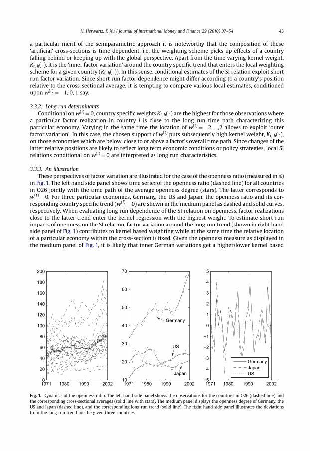
3.3.3. An illustrationThese perspectives of factor variation are illustrated for the case of the openness ratio (measured in %)

in Fig. 1. The left hand side panel shows time series of the openness ratio (dashed line) for all countriesin O26 jointly with the time path of the average openness degree (stars). The latter corresponds tow(t)¼ 0. For three particular economies, Germany, the US and Japan, the openness ratio and its cor-responding country specific trend (w(i)¼ 0) are shown in the medium panel as dashed and solid curves,respectively. When evaluating long run dependence of the SI relation on openness, factor realizationsclose to the latter trend enter the kernel regression with the highest weight. To estimate short runimpacts of openness on the SI relation, factor variation around the long run trend (shown in right handside panel of Fig. 1) contributes to kernel based weighting while at the same time the relative locationof a particular economy within the cross-section is fixed. Given the openness measure as displayed inthe medium panel of Fig. 1, it is likely that inner German variations get a higher/lower kernel based

1971 1980 1990 20020

20

40

60

80

100

120

140

160

180

200

1971 1980 1990 200210

20

30

40

50

60

70

1971 1980 1990 2002−5

−4

−3

−2

−1

0

1

2

3

4

5

Germany

Japan

US

GermanyJapanUS

Fig. 1. Dynamics of the openness ratio. The left hand side panel shows the observations for the countries in O26 (dashed line) andthe corresponding cross-sectional averages (solid line with stars). The medium panel displays the openness degree of Germany, theUS and Japan (dashed line), and the corresponding long run trend (solid line). The right hand side panel illustrates the deviationsfrom the long run trend for the given three countries.


weight than factor variations measured for Japan or the US conditional on a relatively high/low degreeof openness (w(t)¼ 1/w(t)¼�1).

3.4. Inference

Inference on state dependence of the SI relation may proceed conditional on some (approximationof) asymptotic properties of the Nadaraya Watson estimator. In semi- and non-parametric modeling,bootstrap approaches have become a widely used toolkit for inferential issues. For univariate factordependent regressions, Cai et al. (2000) advocate a residual based resampling scheme to infer on factordependence against a structurally invariant model specification. Owing to the relatively small sizedavailable samples, residual based resampling might suffer from the instance that, in the boundaries ofthe factor support, functional estimates could become wiggly and at the same time residual estimatesare unreliably small. Similarly, residual estimation could be adversely affected by possible over- orundersmoothing as a consequence of rule of thumb based bandwidth selection. Furthermore, residualbased bootstrap inference could lack robustness owing to possibly heterogenous error terms. In light ofthe latter caveats, we apply the so-called factor based bootstrap approach (Herwartz and Xu, 2008c)where underlying factors are drawn with replacement.

The adopted approach to contrast a structurally invariant model against the local formalization isimplemented along the following lines:

(1) The local estimate in (7) can be seen as a function of the data and the chosen bandwidth parameter, i.e.

bbðuÞ ¼ fn

yit ; x0it ;uit ¼

�wðiÞit ;w

ðtÞit

�;h; i ¼ 1;.;N; t ¼ 1;.; T

o: (8)

(2) To distinguish the cases of factor dependence and factor invariance of the SI relation we comparelocal estimates with bootstrap counterparts

bb�ðuÞ ¼ fn

yit ; x0it ;u

�it ¼

�wði�Þit ;wðt�Þit

�;h; i ¼ 1;.;N; t ¼ 1;.; T

o; (9)

where bivariate tuples uit*¼ (wit(i*), wit

(t*)) are drawn with replacement from the set of bivariate vari-ables uit¼ (wit

(i), wit(t)). Since sample information on the yit and xit

0 is not affected by the bootstrap, theadopted scheme will disconnect any potential link between the selected factor variable on the onehand and the investment ratio on the other hand. If the true underlying SI relation is state invariant,estimates bbðuÞ and bb�ðuÞ are likely to differ only marginally over the support of the state variable.

(3) Drawing a large number, R¼ 1000 say, of bootstrap estimates bb�ðuÞ allows to decide if the nullhypothesis of a state invariant SI relation can be rejected conditional on some state u¼ (w(i), w(t)).For this purpose, estimates bbðuÞ are contrasted with a confidence interval constructed from itsbootstrap distribution bb�ðuÞ. For this study, we use the 2.5% and 97.5% quantiles of bb�ðuÞ as a 95%confidence interval to hold for the parameter b (u) under the null hypothesis of state invariance.Accordingly, we regard the actual estimate to differ locally from the unconditional relation with 5%significance if bbðuÞ is not covered by the bootstrap confidence interval.

Alternatively, state dependent and invariant model representations could be contrasted by means ofcross-validation (CV) criteria (Allen, 1974). Applying this approach indicates mostly gains in jackknifeforecasting offered by the state dependent model. Due to space considerations the results are notprovided but available from the authors upon request.


3.5. Joint endogeneity and spurious regressions

As has been mentioned, domestic saving might be endogenous in a regression specification ofdomestic investment. Moreover, both the saving and investment ratio might be non-stationary. Thesetwo issues are considered in this subsection, respectively.

First, an alternative semiparametric estimator applying instrumental variables is considered toaddress the endogeneity problem. It is obtained as

bbIV

�wðiÞ;wðtÞ

�¼ XN

i¼1

XT

t¼1

xi;t�1x0itKi;hðwðiÞit �wðiÞÞKt;hðw

ðtÞit �wðtÞÞ

!�1

� XN

i¼1

XT

t¼1

xi;t�1yitKi;h


�Kt;h


�!; ð10Þ

with xi, t�1¼ (1, t, Si*, t�1)0 as vector of instruments. Since a stochastic shock to the investment at timeperiod t shall not be correlated with the saving in period t� 1, bbIV ðwðiÞ;wðtÞÞ in (10) is likely immunizedagainst potential endogeneity of domestic saving.

Second, the potential non-stationarity of the saving or investment ratio can lead to biased estimates.For testing stationarity of disturbance processes in functional coefficient models, we consider thefollowing parametric specification,

I�it ¼�

a1 þ a2wit þ a3w2it

�þ�

d1 þ d2wit þ d3w2it

�t þ

�b1 þ b2wit þ b3w2

it

�S�it þ eit (11)

To identify potential spurious regressions, the null hypothesis of no cointegration between domesticsaving, investment, and factor variables is tested. We apply panel cointegration tests proposed by Kao(1999) for the case of homogenous parameters except the intercept. Thus, a modified version of Eq. (11)with cross-sectional intercept a1i instead of a1 is adopted.

4. Results

In this section, we report results obtained from the state dependent model (4). Potential factorvariables are chosen following economic theories of saving and investment (Debelle and Faruqee, 1996)and core empirical contributions on CA determinants (Edwards, 1995; Milesi-Ferretti and Razin, 1997,1998; Chinn and Prasad, 2003). Moreover, we consider the set of factor variables reflecting the debateon the FH puzzle such as indicators of capital mobility. In addition, proxies for other cross-marketfrictions are evaluated with respect to their explanatory content for worldwide SI relations. A list offactor variables is provided in Appendix 1.

Since functional estimates bbðwðiÞ;wðtÞÞ and bbIV ðwðiÞ;wðtÞÞ from (7) and (10) turn out similar andqualitatively identical, only the former are provided. Furthermore, the modified version of Eq. (11) isapplied for O26 with the openness and age dependency ratio as the factor. These two variables have beenused since they provide the most balanced sample. For three countries quotes of the openness ratio in2002 are not available. These missing values are estimated by means of univariate autoregressive modelsof order 1 with intercept. Applying the Dickey–Fuller t- and r-test statistic suggested in Kao (1999), the nullhypothesis of no cointegration is throughout rejected at the 1% significance level.4 Thus, our analysis doesnot suffer from spurious regression even under potential non-stationarity of saving or investment ratios.

The following discussion does not cover local estimates of the intercept ðbaðuÞÞ and trend parameterðbdðuÞÞ of the model. Rather we concentrate on the empirical features of the SI relation, i.e. on localestimates bbðuÞ. We also estimated the local model excluding the deterministic trend term. Instead ofproviding any explicit results obtained from these exercises for space considerations, we confirm thatfunctional relationships turn out to be invariant in shape under inclusion or exclusion of

4 Gauss package, NPT 1.3, developed by M.-H. Chiang and C. Kao is applied for the panel cointegration tests. Detailed resultsare not provided due to space consideration.


a deterministic trend. For most factors, however, slopes of functional forms are more pronounced forthe model without deterministic trend. In addition, evaluating estimation uncertainty by means ofresampling schemes yields confidence intervals for the SI relation which are throughout wider for thefunctional regression model including the deterministic trend term.

4.1. Factors impacting on saving, investment or the current account

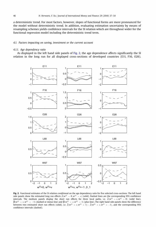
4.1.1. Age dependency ratioAs displayed in the left hand side panels of Fig. 2, the age dependence affects significantly the SI

relation in the long run for all displayed cross-sections of developed countries (E11, F16, O26).

−0.5

0

0.5

1

−1

0

1

2

0

0.5

1

1.5

−0.5

0

0.5

1

−1

0

1

2

0

0.5

1

1.5

−0.5

0

0.5

1

0

0.5

1

−2 −1 0 1 20

0.5

1

w(i)=v, w(t)=−1 ,0 ,1

−2

−1

0

1E11

−1

0

1F16

−2

−1

0

1O26

−1

0

1L68

−2 −1 0 1 2−0.5

0

0.5W97

−2 −1 0 1 2 0

0.5

1

w(i)=0, w(t)=v

E11E11

F16F16

O26O26

L68L68

W97W97

Fig. 2. Functional estimates of the SI relation conditional on the age dependency ratio for five selected cross-sections. The left handside panels show the estimated long run effects bbðwðiÞ ¼ 0;wðtÞ ¼ vÞ (solid). Dashed lines are the corresponding 95% confidenceintervals. The medium panels display the short run effects for three local paths, i.e. bbðwðiÞ ¼ v;wðtÞ ¼ 0Þ (solid line),bbðwðiÞ ¼ v;wðtÞ ¼ �1Þ (dashed or minus line) and bbðwðiÞ ¼ v;wðtÞ ¼ 1Þ (plus line). The right hand side panels show the differencebetween two estimated short run effects (solid), i.e. bbðwðiÞ ¼ v;wðtÞ ¼ 1Þ � bbðwðiÞ ¼ v;wðtÞ ¼ �1Þ, and the corresponding 95%confidence intervals (dashed).


Conditional on country specific long run trends (w(i)¼ 0), the empirical SI relation is decreasing in timespecific age dependency ðwðtÞit ¼ ðewit �wtÞ=stðewÞÞ.

The observed negative impact of the age dependency ratio on the SI relation is consistent with the‘‘Life Cycle Hypothesis’’ (LCH) suggested by Modigliani and Brumberg (1954). According to this theory,consumption or saving is affected by the age distribution of the population. Most households do nothave a constant flow of income over their lifetimes. In order to smooth their consumption path, youngagents should borrow and retired agents shall finance themselves from their past savings. Therefore, ifthe ratio of the dependent population to the working-age population, is high, the aggregate saving rateshall be low. The latter might disconnect the links between domestic saving and investment. In theempirical literature (Modigliani, 1970; Masson et al., 1998) the influence of the age dependency ratio onthe saving ratio has been mainly confirmed by means of studies with cross-country or pooled data.

Regarding the level of the functional SI relations, it is worthwhile to point out that the betweenestimates given in Table 1 are likely not representative for the entire cross-sections. For instance, theestimated between coefficient for E11, bb ¼ �0:16, is far below the SI relation measured over states ofa relatively low age dependency. As such, homogenous models like (1) run the risk of providing biasedapproximations of the link between domestic saving and investment. Note that the latter caveat ofa homogenous model formalization may also be illustrated with other potential factor variables.

For less developed economies (L68), the estimated SI relation shows a U-shaped behavior wheninterpreted as a function of the age dependency ratio. To explain this result, one may conjecture that forless developed economies age dependence affects saving (consumption smoothing) and investment(growth prospect) in a more symmetric fashion than implied by the LCH for developed economies. Asthe most comprehensive cross-section, the results for the long run SI relation given for W97 can beseen as an aggregate over the features of developed (O26) and less developed (L68) economies with thelatter introducing some mild, i.e. insignificant, U-shaped pattern. In sum, the results for W97 under-score that the negative impact of age dependence on the SI relation dominates according to thesignificantly decreasing functional estimates over the factor support �2�w(t)� 0.5.

Effects of short run variations in the age dependency on the SI relation are not observed (mediumpanels of Fig. 2). Conditional on (w(t)¼�1, 0, 1) the estimated functional forms are more or lessconstant. However, comparing conditional estimates for w(t)¼ 1 and w(t)¼�1, it turns out that theformer are almost uniformly below the latter for developed economies (E11, F16, O26). The right handside panels show the difference between these two estimated short run effects, i.e.bbðwðiÞ ¼ v;wðtÞ ¼ 1Þ � bbðwðiÞ ¼ v;wðtÞ ¼ �1Þ, and the corresponding 95% confidence intervals. Thesignificantly negative difference is confirmed for E11 and F16 over the supports �1�w(i)� 1 and forO26 given �2�w(i)� 1.6.

Similar to the latter results on the short run behavior of the SI relation conditional on age depen-dency, analyses conditional on other factors also reveal that the link between domestic saving andinvestment is mostly stable in response to inner country factor variation. For this reason, weconcentrate in the following on the functional relations characterizing the SI relation in the long run.

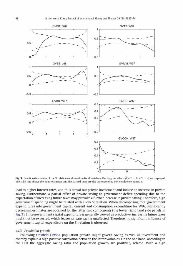
4.1.2. Fiscal variablesFirstly, the government budget balance is considered as a fiscal variable which might have an

influence on the SI relation. A full offset of private saving to government deficits (Ricardian equiva-lence) is generally rejected in the empirical literature. Bernheim (1987) shows that a unit increase inthe government deficit is related with a decrease in consumption of 0.5–0.6. This evidence supports theview that government deficits might be positively correlated with CA deficits, thereby describing so-called ‘‘Twin Deficits’’. Based on this argument, we shall expect a hump-shaped SI relation conditionalon an increasing government budget balance since a high CA imbalance is consistent with a low SIrelation. Although a significant left part of a hump shape is found for developed economies (O26),a significant influence of the government budget balance on the SI relation is not observed for W97, ascan be seen in the left hand side panels of Fig. 3.

In the second place, we consider the influence of the composition of government expenditures onthe SI relation. As can be seen from the upper right hand side panel of Fig. 3, a significantly decreasingestimated SI relation is obtained for W97 conditional on increasing total government expenditure. Forthe remaining cross-sections, similar effects are found. A higher government deficit spending might

0

0.5

1GVBB: O26

−0.5

0

0.5

1GVBB: L68

−2 −1 0 1 2−0.5

0

0.5

1GVBB: W97

−0.5

0

0.5

1GVTT: W97

−0.5

0

0.5

1GVIVM: W97

−0.2

0

0.2

0.4

0.6GVCE: W97

−2 −1 0 1 20

0.2

0.4

0.6

0.8GVCON: W97

Fig. 3. Functional estimates of the SI relation conditional on fiscal variables. The long run effects bbðwðiÞ ¼ 0;wðtÞ ¼ vÞ are displayed.The solid line shows the point estimates and the dashed lines are the corresponding 95% confidence intervals.


lead to higher interest rates, and thus crowd out private investment and induce an increase in privatesaving. Furthermore, a partial offset of private saving to government deficit spending due to theexpectation of increasing future taxes may provoke a further increase in private saving. Therefore, highgovernment spending might be related with a low SI relation. When decomposing total governmentexpenditures into government capital, current and consumption expenditure for W97, significantlydecreasing estimates are obtained for the latter two components (the lower right hand side panels inFig. 3). Since government capital expenditure is generally viewed as productive, increasing future taxesmight not be expected, which leaves private saving unaffected. Therefore, no significant influence ofgovernment capital expenditure on the SI relation is observed.

4.1.3. Population growthFollowing Obstfeld (1986), population growth might govern saving as well as investment and

thereby explain a high positive correlation between the latter variables. On the one hand, according tothe LCH the aggregate saving ratio and population growth are positively related. With a high


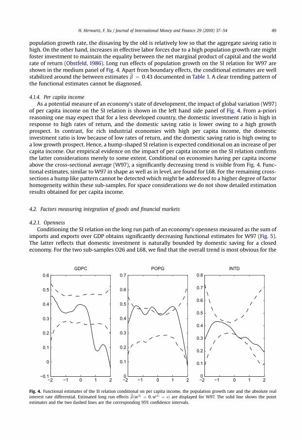
population growth rate, the dissaving by the old is relatively low so that the aggregate saving ratio ishigh. On the other hand, increases in effective labor forces due to a high population growth rate mightfoster investment to maintain the equality between the net marginal product of capital and the worldrate of return (Obstfeld, 1986). Long run effects of population growth on the SI relation for W97 areshown in the medium panel of Fig. 4. Apart from boundary effects, the conditional estimates are wellstabilized around the between estimates bb ¼ 0:43 documented in Table 1. A clear trending pattern ofthe functional estimates cannot be diagnosed.

4.1.4. Per capita incomeAs a potential measure of an economy’s state of development, the impact of global variation (W97)

of per capita income on the SI relation is shown in the left hand side panel of Fig. 4. From a-priorireasoning one may expect that for a less developed country, the domestic investment ratio is high inresponse to high rates of return, and the domestic saving ratio is lower owing to a high growthprospect. In contrast, for rich industrial economies with high per capita income, the domesticinvestment ratio is low because of low rates of return, and the domestic saving ratio is high owing toa low growth prospect. Hence, a hump-shaped SI relation is expected conditional on an increase of percapita income. Our empirical evidence on the impact of per capita income on the SI relation confirmsthe latter considerations merely to some extent. Conditional on economies having per capita incomeabove the cross-sectional average (W97), a significantly decreasing trend is visible from Fig. 4. Func-tional estimates, similar to W97 in shape as well as in level, are found for L68. For the remaining cross-sections a hump like pattern cannot be detected which might be addressed to a higher degree of factorhomogeneity within these sub-samples. For space considerations we do not show detailed estimationresults obtained for per capita income.

4.2. Factors measuring integration of goods and financial markets

4.2.1. OpennessConditioning the SI relation on the long run path of an economy’s openness measured as the sum of

imports and exports over GDP obtains significantly decreasing functional estimates for W97 (Fig. 5).The latter reflects that domestic investment is naturally bounded by domestic saving for a closedeconomy. For the two sub-samples O26 and L68, we find that the overall trend is most obvious for the

−2 −1 0 1 2−0.1

0

0.1

0.2

0.3

0.4

0.5

0.6GDPC

−2 −1 0 1 20

0.1

0.2

0.3

0.4

0.5

0.6

0.7POPG

−2 −1 0 1 20

0.1

0.2

0.3

0.4

0.5

0.6

0.7

0.8INTD

Fig. 4. Functional estimates of the SI relation conditional on per capita income, the population growth rate and the absolute realinterest rate differential. Estimated long run effects bbðwðiÞ ¼ 0;wðtÞ ¼ vÞ are displayed for W97. The solid line shows the pointestimates and the two dashed lines are the corresponding 95% confidence intervals.

0

0.5

1F16

0

0.5

1

1.5O26

0

0.2

0.4

0.6

0.8L68

−2 −1 0 1 20

0.5

1W97

IMPT

−0.5

0

0.5

1F16

0.2

0.4

0.6

0.8

1O26

0

0.2

0.4

0.6

0.8L68

−2 −1 0 1 2−0.5

0

0.5

1W97

EXPT

−0.5

0

0.5

1F16

0

0.5

1O26

0

0.2

0.4

0.6

0.8L68

−2 −1 0 1 20

0.5

1W97

OPN

Fig. 5. Functional estimates of the SI relation conditional on the openness ratio, the ratio of exports and imports to GDP for threeselected cross-sections. Estimated long run effects bbðwðiÞ ¼ 0;wðtÞ ¼ vÞ are displayed. The solid line shows the point estimates andthe two dashed lines are the corresponding 95% confidence intervals.


group of less developed economies. This impression might mirror that L68 is likely more heterogenouswith regard to country specific degrees of openness. Considering the 16 OECD members in F16,nevertheless, the decreasing trend is evident as well. By construction, the ‘openness’ variable isa measure reflecting good markets integration. As such, our results motivate the view that the SIrelation is perhaps not only reflecting capital market separation as stated by FH (1980) but also barriersof international trade (Obstfeld and Rogoff, 2000). Furthermore, when alternatively decomposing theopenness measure in its two components, exports over GDP and imports over GDP, they have ratherdifferent impacts on the SI relation for less developed economies (L68). This dominant effect can befurther observed in the world sample (W97). By definition, exports over GDP describe the surplus indomestic output provided to the rest of the world while imports over GDP indicate the dependency ofa country on foreign goods. It turns out that the closeness of less developed economies is likely stronger


signalled by its low dependency on the foreign products (import ratios) than by its low productionsurplus (export ratios). As can be seen in Fig. 5, the SI relation is significantly high when standardizedimport ratios are around �2<w(t)<�1.

4.2.2. Interest rate parityHaving discussed the impact of openness as a measure of good markets integration on the SI

relation it is also tempting to relate this relation to some measure approximating capital marketintegration. For this purpose we use the absolute real interest rate differential measured for a particulareconomy towards a world real interest rate index. Country specific real interest rates are the lendingrates charged by banks on loans to prime customers adjusted for inflation. To approximate the realworld interest rate we construct a GDP weighted average of real interest rates among the US, Germanyand Japan. Instead of using the interest rate differential directly we presume that positive and negativerealizations are equally informative for the prevalence of capital market frictions. Therefore weinvestigate the impact of the absolute real interest differential on the SI relation. As documented in theright hand side panel of Fig. 4, a significant impact of the real interest rate differential on the SI relationfor W97 is not found in our analysis for the global perspective, which is also representative for allremaining cross-sections (not shown for space considerations). Still, however, one may regard thedifferent unconditional levels of empirical SI relations as reported in Table 1, for E11 against O15 say, tosignal a mitigating impact of market integration on the SI relation.

By using the real interest rate differential, we are aware that this measure might not only corre-spond to capital mobility, as argued by Frankel (1992). As another potential measure of capital mobility,we consider the nominal interest rate differential. However, significant impacts of this measure on theSI relation are likewise not obtained.

4.3. Large country effect

As can be seen in Fig. 6, significantly positive long run impacts of the log GDP on the SI relation canbe diagnosed for E11, O26 and W97, thereby supporting a large country effect. A large country mighthave a higher SI relation than a small country owing to an endogenous domestic interest rate. For the

−2 −1 0 1 2−0.2

−0.1

0

0.1

0.2

0.3

0.4

0.5

0.6

0.7E11

−2 −1 0 1 20.2

0.3

0.4

0.5

0.6

0.7

0.8

0.9

1O26

−2 −1 0 1 20.1

0.2

0.3

0.4

0.5

0.6

0.7

0.8

0.9W97

Fig. 6. Functional estimates of the SI relation conditional on the logarithm of GDP. Estimated long run effects bbðwðiÞ ¼ 0;wðtÞ ¼ vÞare displayed. The solid line shows the point estimates and the two dashed lines are the corresponding 95% confidence intervals.


cross-section of less developed economies we cannot confirm a large country effect which might beexpected given that L68 collects small economies by definition.

To summarize the results in this section, according to functional coefficient estimates the SI relationis found to be rather stable in the short run, but factor dependent in the long run. A low SI relationmight be due to a high degree of the trade openness, a high age dependency ratio, or high governmentcurrent and consumption expenditures. In addition, small countries tend to have a lower SI relation incomparison with larger economies.

In light of the diagnosed factor dependent nature of empirical SI relations it is natural to address itspotential implications. Firstly, the increasing integration of capital markets alone does not automati-cally decrease the correlation between domestic saving and investment. The integration of globalcapital markets is necessary but not sufficient for a high net capital in/out-flow and thus a low SIrelation. The extent to which domestic saving and investment are disconnected depends on variablesas the openness ratio, the age dependency ratio and government current and consumption expendi-tures according to our analysis. Economies with high age dependency ratios or high exports have moremoney to lend and thus seek internationally the highest return. Comparably, economies with highgovernment consumption and current expenditures or high imports might have more incentive toborrow internationally at the lowest costs. For these economies the SI relation may be low. Secondly,since a low SI relation tends to correspond to a high CA imbalance, determinants of the SI relation canalso be regarded as determinants of the CA. Based on our results, high government current andconsumption expenditure may induce a high CA imbalance for most economies. For OECD countries,a high CA imbalance might go along with a high age dependency ratio. Furthermore, the increasingdegree of openness in goods markets might provide countries with the possibility to sustain long runCA imbalances.

5. Conclusions

In this paper we investigate the relation between domestic saving and investment for seven cross-sections covering the sample period 1971–2002. A new framework of bivariate functional coefficientmodels is applied to estimate conditional SI relations. A factor based resampling scheme is adopted toaddress inferential issues for the new model. Our bivariate functional approach allows to separatefactor dependence of the SI relation in the short and long run. In the short run, factor dependent SIrelations are found to be rather stable. In the long run, however, a set of economic factors is found toimpact the SI relation. The latter are an economy’s openness ratio, the age dependency ratio andgovernment expenditures. Supporting evidence for a large country effect is also found. According tothese results, the interpretation of a high SI relation as a signal for low capital mobility in FH (1980) hasto be treated with care.

Acknowledgements

The authors thank an anonymous referee and participants in seminars at the Free University Berlin,the University of Maastricht and the International Conference on Policy Modeling in Hong Kong, 2006,for helpful suggestions. Financial support of Fritz Thyssen Stiftung (Az.10.08.1.088) is also gratefullyacknowledged.

Appendix 1. List of factors

Group 1

AGE: Ratio of the dependent population (younger than 15 and older than 64) to the working-agepopulation (between 15 and 64) (%).

GVBB: Ratio of government overall budget balance (including grants) to GDP (%).GVTT: Ratio of government total expenditure to GDP (%).GVIVM: Ratio of government capital expenditure to GDP (%).


GVCE: Ratio of government current expenditure to GDP (%).GVCON: Ratio of government consumption expenditure to GDP (%).POPG: Growth rate of the population (%).GDPC: Natural logarithm of GDP per capita.

Group 2

OPN: Ratio of export plus import to GDP (%).EXPT: Ratio of exports of goods and services to GDP (%).IMPT: Ratio of imports of goods and services to GDP (%).INTD: Absolute real interest rate differential measured for a particular economy towards a world

real interest rate index (%).

Group 3

GDP: Natural logarithm of GDP.

Appendix 2. List of countries included in W97

Algeria; Argentina; Australia; Austria; Bangladesh; Barbados; Belgium; Benin; Botswana; Brazil;Burkina Faso; Burundi; Cameroon; Canada; Central African Republic; Chile; China; Colombia; CongoDem. Rep.; Congo Rep.; Costa Rica; Ivory Coast; Denmark; Dominican Republic; Ecuador; Egypt ArabRep.; El Salvador; Fiji; Finland; France; Gabon; Gambia; Germany; Ghana; Greece; Guatemala; Guyana;Haiti; Honduras; Hong Kong, China; Hungary; Iceland; India; Indonesia; Ireland; Israel; Italy; Jamaica;Japan; Kenya; Korea, Rep.; Kuwait; Luxembourg; Madagascar; Malawi; Malaysia; Mali; Malta;Mauritania; Mexico; Morocco; Myanmar; Nepal; Netherlands; New Zealand; Niger; Nigeria; Norway;Pakistan; Paraguay; Peru; Philippines; Portugal; Rwanda; Saudi Arabia; Senegal; Singapore; SouthAfrica; Spain; Sri Lanka; Suriname; Swaziland; Sweden; Switzerland; Syrian Arab Republic; Thailand;Togo; Trinidad and Tobago; Tunisia; Turkey; Uganda; United Kingdom; United States; Uruguay;Venezuela, RB; Zambia; Zimbabwe.

References

Abbott, A., Vita, G.D., 2003. Another piece in the Feldstein–Horioka puzzle. Scottish Journal of Political Economy 50, 69–89.Allen, D.M., 1974. The relationship between variable selection and data augmentation and a method for prediction. Techno-

metrics 16, 125–127.AmirKhalkhali, S., Dar, A.A., AmirKhalkhali, S., 2003. Saving–investment correlations, capital mobility and crowding out: some

further results. Economic Modelling 20, 1137–1149.Artis, M., Bayoumi, T., 1992. Global capital market integration and the current account. In: Taylor, M. (Ed.), Money and Financial

Markets. Blackwell, Cambridge, MS and Oxford, pp. 297–307.Bajo-Rubio, O., 1998. The saving–investment correlation revisited: the case of Spain, 1964–1994. Applied Economics Letters 5,

769–772.Bernheim, B.D., 1987. Ricardian equivalence: an evaluation of theory and evidence. In: Fischer, S. (Ed.), NBER Macroeconomics

Annual 1987. MIT Press, Cambridge.Blanchard, O., Giavazzi, F., 2002. Current Account Deficits in the Euro Area. The End of the Feldstein Horioka Puzzle? MIT

Department of Economics. Working Paper 03-05.Cai, Z., Fan, J., Yao, Q., 2000. Functional-coefficient regression models for nonlinear time series. Journal of the American

Statistical Association 95, 941–956.Chinn, M., Prasad, E.S., 2003. Medium-term determinants of current accounts in industrial and developing countries: an

empirical exploration. Journal of International Economcis 59, 47–76.Coakley, J., Fuertes, A.-M., Spagnolo, F., 2004. Is the Feldstein–Horioka puzzle history? The Manchester School 72, 569–590.Coakley, J., Kulasi, F., Smith, R., 1996. Current account solvency and the Feldstein–Horioka puzzle. Economic Journal 106, 620–

627.Coakley, J., Kulasi, F., Smith, R., 1998. The Feldstein–Horioka puzzle and capital mobility: a review. International Journal of

Finance and Economics 3, 169–188.Coiteux, M., Olivier, S., 2000. The saving retention coefficient in the long run and in the short run. Journal of International

Money and Finance 19, 535–548.Debelle, G., Faruqee, H., 1996. What Determines the Current Account? A Cross-sectional and Panel Approach. IMF Working

Paper no. 96/58. IMF.


Edwards, S., 1995. Why are Saving Rates So Different Across Countries? An International Comparative Analysis. NBER WorkingPaper 5097. NBER.

Feldstein, M., Horioka, C., 1980. Domestic saving and international capital flows. Economic Journal 90, 314–329.Frankel, J.A., 1992. Measuring international capital mobility: a review. American Economic Review 82 (2), 197–202.Gulley, O.D., 1992. Are saving and investment cointegrated? Economics Letters 39, 55–58.Haan, J.D., Siermann, C.L.,1994. Saving, investment, and capital mobility. A comment on Leachman. Open Economies Review 5, 5–17.Hardle, W., Hall, P., Marron, J.S., 1988. How far are automatically chosen regression smoothing parameters from their optimum?

Journal of the American Statistical Association 83, 86–99.Herwartz, H., Xu, F., 2008a. Reviewing the sustainability/stationarity of current account imbalances with tests for bounded

integration. The Manchester School 76, 267–278.Herwartz, H., Xu, F., 2008b. Panel data model comparison for the investigation of the saving–investment relation. Applied

Economic Letters. doi:10.1080/13504850701221949.Herwartz, H., Xu, F., 2008c. A new approach to bootstrap inference in functional coefficient models. Computational Statistics

and Data Analysis. doi:10.1016/j.csda.2008.09.014.Ho, T.-W., 2002a. The Feldstein–Horioka puzzle revisited. Journal of International Money and Finance 21, 555–564.Ho, T.-W., 2002b. A panel cointegration approach to the investment–saving correlation. Empirical Economics 27, 91–100.Hodrick, R.J., Prescott, E.C., 1997. Postwar U.S. business cycles: an empirical investigation. Journal of Money, Credit and Banking

29, 1–16.Jansen, W.J., 1996. Estimating saving–investment correlations: evidence for OECD countries based on an error correction model.

Journal of International Money and Finance 15, 749–781.Jansen, W.J., 1998. Interpreting saving–investment correlations. Open Economies Review 9, 205–217.Jansen, W.J., 2000. International capital mobility: evidence from panel data. Journal of International Money and Finance 19, 507–511.Jansen, W.J., Schulze, G.G., 1996. Theory-based measurement of the saving–investment correlation with an application to

norway. Economic Inquiry 34, 116–132.Kao, C., 1999. Spurious regrsesion and residual-based tests for cointegration in panel data. Journal of Econometrics 90, 1–44.Kasuga, H., 2004. Saving–investment correlations in developing countries. Economics Letters 83, 371–376.Leachman, L.L., 1991. Saving, investment, and capital mobility among OECD countries. Open Economies Review 2, 137–163.Lemmen, J.J., Eijffinger, S.C., 1995. The quantity approach to financial integration: the Feldstein–Horioka criterion revisited. Open

Economies Review 6, 145–165.Masson, P.R., Bayoumi, T., Samiei, H., 1998. International evidence on the determinants of private saving. The World Bank

Economic Review 12, 483–501.Milesi-Ferretti, G.M., Razin, A., 1997. Sharp Reductions in Current Account Deficits: an Empirical Analysis. NBER Working Paper

6310. NBER.Milesi-Ferretti, G.M., Razin, A., 1998. Current Account Reversals and Currency Crises: Empirical Regularities. NBER Working

Paper 6620. NBER.Miller, S.M., 1988. Are saving and investment cointegrated? Economics Letters 27, 31–34.Modigliani, F., 1970. The life-cycle hypothesis of saving and intercountry differences in the saving ratio. In: Eltis, W., Scorr, M.,

Wolfe, J. (Eds.), Induction, Trade, and Growth: Essays in Honour of Sir Roy Harrod. Clarendon Press, Oxford.Modigliani, F., Brumberg, R., 1954. Utility analysis and the consumption function: an interpretation of cross-section data. In:

Kurihara, K.K. (Ed.), Post-Keynesian Economics. Rutgers University Press.Moreno, R., 1997. Saving–investment dynamics and capital mobility in the US and Japan. Journal of International Money and

Finance 16, 837–863.Nadaraya, E., 1964. On estimating regression. Theory of Probability and Its Applications 10, 186–190.Obstfeld, M., 1986. Capital mobility in the world economy: theory and measurement. Carnegie-Rochester Conference Series on

Public Policy 24, 55–104.Obstfeld, M., Rogoff, K., 2000. The six major puzzles in international macroeconomics: is there a common cause? In: Ber-

nanke, B.S., Rogoff, K. (Eds.), NBER Macroeconomics Annual 2000. MIT Press, pp. 339–390.Ozmen, E., Parmaksiz, K., 2003a. Exchange rate regimes and the Feldstein–Horioka puzzle: the French evidence. Applied

Economics 35, 217–222.Ozmen, E., Parmaksiz, K., 2003b. Policy regime change and the Feldstein–Horioka puzzle: the UK evidence. Journal of Policy

Modeling 25, 137–149.Pelagidis, T., Mastroyiannis, T., 2003. The saving–investment correlation in greece, 1960–1970: implications for capital mobility.

Journal of Policy Modeling 25, 609–616.Pelgrin, F., Schich, S., 2004. National Saving–Investment Dynamics and International Capital Mobility. Working Paper 2004-14.

Bank of Canada.Ravn, M.O., Uhlig, H., 2002. Onadjusting the HP-filter for the frequency of observations. Review of Economics and Statistics 84, 371–380.Sachsida, A., Caetano, M.A.-R., 2000. The Feldstein–Horioka puzzle revisited. Economics Letters 68, 85–88.Schmidt, M.B., 2001. Savings and investment: some international perspectives. Sourthern Economic Journal 68, 446–456.Scott, D.W., 1992. Multivariate Density Estimation: Theory, Practice, and Visualization. John Wiley & Sons, New York, Chichester.Sinha, T., Sinha, D., 2004. The mother of all puzzles would not go away. Economics Letters 82, 259–267.Summers, L.H., 1988. Tax policy and international competitiveness. In: Frankel, J. (Ed.), International Aspects of Fiscal Polices.

University of Chicago Press, Chicago, pp. 349–386.Taylor, A.M.,1996. International Capital Mobility in History: the Saving–Investment Relationship. NBER Working Paper 5743. NBER.Taylor, A.M., 1998. Argentina and the world capital market: saving, investment, and international capital mobility in the

twentieth centruy. Journal of Development Economics 57, 147–184.Taylor, A.M., 2002. A Century of Current Account Dynamics. NBER Working Paper 8927. NBER.Tesar, L.L., 1993. International rsik-sharing and non-traded goods. Journal of International Economics 35, 69–89.Vita, G.D., Abbott, A., 2002. Are saving and investment cointegrated? An ARDL bounds testing approach. Economics Letters 77,

293–299.Watson, G., 1964. Smooth regression analysis. Sankhy�a, Series A 26, 359–372.

a functional coefficient model view of the feldstein–horioka puzzle

Documents