the feldstein horioka puzzle by groups of oecd members: the

MPRAMunich Personal RePEc Archive

The Feldstein Horioka Puzzle by groupsof OECD members: the panel approach.

N. Natalya Ketenci

Yeditepe University

August 2010

Online at https://mpra.ub.uni-muenchen.de/25848/MPRA Paper No. 25848, posted 15. October 2010 00:26 UTC

http://mpra.ub.uni-muenchen.de/

https://mpra.ub.uni-muenchen.de/25848/

1

The Feldstein Horioka Puzzle by groups of OECD members: the panel approach.

Natalya Ketenci1

(Yeditepe University, Istanbul)

Abstract

This paper investigates investment savings relationships in 26 OECD countries and how these

relationships change when countries in the considered panel vary. Therefore panel estimations

using annual data for the period 1970-2008 are made for different groups of developed

countries, such as the OECD, EU15, NAFTA and G7. Additionally, this paper examines

changes in investment saving relationships in groups of developed countries taking into

account the presence of structural shifts in countries where they exist. Recent panel

techniques are employed in this study to examine investment savings relationships and to

estimate saving retention coefficients. The empirical findings reveal that the Feldstein-

Horioka puzzle exists only in the panel of G7 countries where the saving-retention coefficient

is estimated at the level 0.754 and 0.864 for the full sample of G7 countries and for stable

countries, respectively. The estimated saving-retention coefficient for the G7 group of

unstable appear at the 0.482 level, indicating a higher level of capital mobility in unstable

countries compared to stable ones. This conclusion is supported by estimations for OECD and

EU15 countries.

JEL: F32Key Words: Feldstein-Horioka puzzle, capital mobility, structural breaks, panel estimations,OECD.

1 Natalya Ketenci, Department of Economics, Yeditepe University, Kayisdagi, 34755, Istanbul, Turkey. Tel: 0090 5780581. Fax: 0090 5780797. E-mail: [email protected].

Created with Print2PDF. To remove this line, buy a license at: http://www.software602.com/

2

1. Introduction

For last three decades numerous studies have been carried out in attempts to explain and to

solve the Feldstein Horioka puzzle. The phenomenon of the Feldstein Horioka puzzle (FHP)

is related to the seminal work of Feldstein and Horioka (1980). In their study they found that

investment and saving ratios are correlated highly in developed countries, which is an

illustration of low capital mobility. These findings are opposite to the expected low

correlation between investment and savings ratios particularly in the sample of the OECD

developed countries. Since then in the literature a great deal of attention has been given to the

FHP (see, for example, literature surveys by Frankel [1992], Coakley et al. [1998], and

Apergis and Tsoumas [2009]).

Studies on FHP differ in terms of methodology and in terms of different econometric

techniques as well, where cross-sectional data (see Feldstein-Horioka [1980], Murphy [1984],

Penati and Dooley [1984], Dooley et al. [1987], Coakley et al. [1998], Herwartz and Xu

[2010]), time-series (see Miller [1988], Argimon and Roldan [1994], Jansen [1996], Coakley

and Kulasi [1997], Caporale et al. [2005]) as well as panel data (see Corbin [2001], Ho

[2002], Fouquau et al. [2008], Kollias et al. [2008], Georgopoulos and Hejazi [2009],

Vasudeva Murthy [2009], Rao et al. [2010], Herwartz and Xu [2010] ) were employed.

Empirical studies using panel data vary in their results according to different applied

econometric techniques. For example, Fouquau et al. (2008) in a panel study on 23 OECD

countries used the panel smooth transition regression model, where the saving-retention

coefficient was broken down into five classes presented by factors that mostly have an effect

on countries’ capital mobility. These factors are economic growth, demography, degree of

openness, country size and current account balance. The results of this study indicate the

strong heterogeneity in the capital mobility of developed countries. It was found as well that

the estimated coefficients for the OECD sample fall generally between the years 1960 and

2000.

Kollias et al. (2008) employed the bounds testing procedure to test for the presence of

cointegration in a cross-sectional sample of 15 European Union members for the 1962-2002

period. At the same time, the authors applied panel data techniques to test for individual and

temporal effects in the sample. The results indicated that the country specific parameter is a

random variable, while the time specific parameter is a fixed variable with the saving-

retention coefficient being at a level between 0.148-0.157, indicating high capital mobility in

the sample group.


3

Banerjee and Zanghiery (2003) used a sample of 14 European Union members over

the period 1970-2002. They employed the Johansen country-by-country cointegration test and

Pedroni panel cointegration test. The results mostly support the integration hypothesis in the

data series. At the same time, the authors emphasize that the consideration of the groups of

countries and the cross-unit cointegration possibility is essential in the results' sensitivity.

Most empirical studies with panel data have concentrated on large samples of OECD

countries following the work of Feldstein and Horioka (1980) (see, for example, Ho [2002],

Fouquau et al. [2008], Adedeji and Thornton [2008]). Another group of studies narrows its

focus to European Union countries (for example, Banerjee and Zanghieri [2003], Telatar et al.

[2007], Kollias et al. [2008]) or to smaller samples of OECD countries (Georgopoulos and

Hejazi [2009], Rao et al. [2010], Narayan and Narayan [2010]). Another study compares

groups of developed and developing countries (for example, Sinha and Sinha [2004], Adedeji

and Thornton [2008], Herwartz and Xu [2010]). Thus Sinha and Sinha (2004) in their study of

123 countries found evidence for capital mobility for only 16 countries, most of which are

developing countries. Taking into account that macroeconomic series such as investment and

savings are sensitive to economic and political changes domestically as well as world-wide, it

is important to analyze saving-retention coefficients in the presence of structural breaks, if

such exist. However, there are few studies on FHP in OECD members that take into account

the existence of structural shifts. For example, Ozmen and Parmaksiz (2003), Telatar et al.

(2007), Mastroyiannis (2007), Kejriwal (2008) in their studies analyze FHP with the

possibility of structural breaks in individual countries or in cross-sectional samples. Only a

few studies consider structural changes in the panel data of developed countries (for example,

Iorio and Fachin [2007], Telatar et al. [2007], Rao et al. [2010]).

The results of FHP analysis vary with the employed econometric techniques, the

inclusion of structural changes, the employed country samples and with different time

periods. Therefore, it is difficult to make general conclusions on FHP analysis in the literature

due to the absence of homogeneity in studies.

This study employs a sample of OECD countries and makes a comparative analysis of

different groups that are generated from OECD countries. Particularly in this study four

different groups of countries are considered: OECD, EU15, NAFTA and G7. Members of

European Union countries have higher possibility to have homogenous investment saving

relations (see, for example, Blanchard and Giavazzi [2002]). At the same time members of

more narrowed groups such as NAFTA and G7 are more likely to have homogeneous

investment policies as well compared to a wider group of countries such as OECD. The


4

purpose of this study is to examine investment-saving associations and to find out how they

change in different groups of developed countries in the presence of structural breaks where

such exist and in the absence of structural changes when they are not detected. At the same

time, this study compares the results of panel cointegration tests with and without the

inclusion of structural breaks when it is necessary. This study investigates the sensitivity of

results when developed countries are divided into more homogenous groups and when the

existing structural breaks are counted in estimations.

The data sample of this study includes 26 member OECD countries except Chile, Czech

Republic, Hungary, Poland and the Slovak Republic for a lack of homogenous data for these

countries for the full considered period in the used source. The annual data for the 1970-2008

period are extracted from the official statistical site of the OECD. The rest of the paper is

organized as follows. In the next section the applied methodological approach is presented. In

section 3 the obtained empirical results are reported and, finally, the last section concludes.

2. Methodology

This study investigates the degree of capital mobility in OECD members compared to

different narrowed groups of developed countries taking into account identified structural

breaks. In order to examine the level of capital mobility in OECD countries, Feldstein and

Horioka (1980) estimated the following equation:

iii

eYS

YI

(1)

Where I is gross domestic investment, S is gross domestic savings and Y is gross

domestic product of considered country i. Coefficient β, which is known as a saving retention

coefficient, measures the degree of capital mobility. If a country possesses perfect

international capital mobility, the value of β has to be close to 0. If the value of β is close to 1,

it would indicate the capital immobility of the country. The results of Feldstein Horioka

(1980) showed that the value of β for 21 open OECD economies changes between 0.871 and

0.909, illustrating by this the international capital immobility in the considered countries.

These controversial results gave start to widespread debates in the economic literature.

Numerous studies have provided evidence supporting these results. At the same time,

different results exist in the literature with a wide array of interpretations. Therefore, the

findings of Feldstein Horioka (1980), which are contrary to economic theory, have started to

be referred to as “the mother of all puzzles” (Obstfeld and Rogoff, 2000, p.9).


5

In this paper different tests for the panel unit root are used. The first group consists of

tests that do not allow for structural changes in series. These are the Levin, Lin and Chu

(LLC) test (Levin et al., 2002), the Breitung (Breitung, 2000) test, the Im, Pesaran and Shin

(IPS) test (Im et al. 2003), the Fisher-type tests using ADF and PP tests (Maddala and Wu

(1999) and the Choi (2001), and the Hadri (Hadri, 2000) test. The LLC test is based on

orthogonalized residuals and on the correction by the ratio of the long-run to the short-run

variance of each variable. Although the LLC test has become a widely accepted panel unit

root test, it has homogeneity restriction, allowing for heterogeneity only in the constant term

of the ADF regression. The Breitung test assumes that all panels have common a

autoregressive parameter and the presence of the common unit root process. The IPS test is a

heterogeneous panel unit root test based on individual ADF tests and was proposed by Im et

al. (2003) as a solution to the homogeneity issue. This test allows for heterogeneity in both the

constant and slope terms of the ADF regression. Maddala and Wu (1999) and Choi (2001)

proposed an alternative approach by using the Fisher test, which is based on combining the P-

values from the individual unit root test statistics such as ADF and PP. One of the advantages

of the Fisher test is that it does not require a balanced panel. Finally, the Hadri test is a

heterogenous panel unit root test that is an extension of the test of Kwiatkowski et al. (1992),

the KPSS (Kwiatkowski–Phillips–Schmidt–Shin) test, to a panel with individual and time

effects and deterministic trends, which has as its null the stationarity of the series.

However, the considered unit root tests do not take into account the presence of any

structural shifts in series. Therefore, as proposed by Im et al. (2005), the LM unit root test was

employed. This is a panel extension of the Schmidt and Phillips (1992) test allowing for one

and two structural shifts in the trend of a panel and of every individual time series. Im et al.

(2005) illustrated that in the series where structural shifts do not exist the size of distortions

and loss of power in the panel unit root tests remain insignificant when structural shifts are

accommodated. However, size distortions and loss power in the tests were found to be

significant when unit root tests were applied to the time series without taking into account the

existing structural shifts. The break date in the Im et al. (2005) test is chosen using the

minimum LM statistics of Lee and Strazicich (2003, 2004). In this method, the break date is

selected when the t-statistic of possible break points is minimized.

In order to be able to apply panel cointegration tests allowing for structural shifts, it is

necessary to examine series for stability. The Hansen’s (1992) stability test was employed in

this study to estimate parameter stability in cointegration relationships. The test is based on

the fully modified OLS residuals proposed by Phillips and Hansen (1990). A necessary


6

requisite of the test is that series have to be non-stationary. The stability test produces three

test statistics: supF, meanF and Lc. The supF statistic tests for the null hypothesis of

cointegration with no structural shift in the parameter vector against the alternative hypothesis

of cointegration in the presence of sudden structural shifts. The meanF and Lc statistics test

for a cointegration with constant parameters against an alternative hypothesis of gradual

variance in parameters, which is considered no cointegration. Particularly, the meanF statistic

is used to capture the overall stability of the model.

Cointegration tests were employed in this study in order to determine whether long-

run relationships exist between investment and savings. Two of them are the Kao (1999) and

the Pedroni (1999) cointegration tests, which do not allow for structural shifts in series. The

next one is the Westerlund (2006) panel cointegration test, which allows for multiple

structural breaks in series. The following system of cointegrated regressors is considered for

estimation in cointegration tests:

ititiit xy (2)

Where i=1,…, N, and t=1,…., T, αi are constant terms, β is the slope, yit and xit are

non-stationary regressors, and εit are stationary disturbance terms. Kao (1999) proposed two

types of panel cointegration tests, the Dickey-Fuller (DF) and the Augmented Dickey-Fuller

(ADF) tests. The statistics of these tests can be calculated using the following formula:

p

jitjitjitit u

11 (3)

Where the residuals derived in the system (2) are used to calculate the test statistics (3) and to

tabulate the distributions. The null hypothesis of the test is ,1:0 H versus

alternative 1:1 H .

Pedroni (1999) developed a panel and group cointegration test where seven residual-

based tests (with four panel statistics and three group statistics) were introduced in order to

test the hypothesis of no cointegration in dynamic panel series with multiple regressors. The

first four panel cointegration tests, which are defined as within-dimension- based statistics,

use the following null and alternative hypotheses: ,1:0 H 1:1 H , assuming the

homogeneity of coefficients under the null hypothesis. The other three group statistics, which

are defined as between-dimension-based statistics, use ,1:0 iH versus 1:1 iH for all i.

In this case for each ith unit it is necessary to calculate N coefficients i from equation (3),

where slope heterogeneity across countries is now allowed under the alternative hypothesis.


7

In the long run, macroeconomic series such as investment and savings may contain a

variety of structural changes within a country or at the international level. Therefore, in order

to examine the regression model (1) in the case when structural breaks are detected,

Westerlund (2006) methodology is employed in this study. This is the panel cointegration test

that allows for multiple structural breaks accommodation in the level as well as in the trend of

cointegrated regression. This test is based on the panel cointegration residual-based LM test

proposed by McCoskey and Kao (1998), which does not allow for structural shifts. The

advantage of Westerlund’s test is that it allows for the possibility of known a priori multiple

structural breaks or it allows for breaks the locations of which are determined endogenously

from the series. At the same time this test allows for a possibility of structural breaks that may

be placed at different locations in different individual series. Westerlund (2006) showed in his

work that the test is free of nuisance parameters under the null hypothesis and that the number

and location points of structural shifts do not affect the limiting distribution. The null of the

test is 0:0 iH for all ,,....,1 Ni versus alternative hypothesis: 0:1 iH for

,,....,1 1Ni and 0i for .,....,11 NNi One of important advantages of this test is that

the alternative hypothesis is not just a general rejection of the null like in the commonly used

LM panel cointegration test of McCoskey and Kao (1998), but allows i to differ across

individual series.

Finally, in order to estimate saving-retention coefficients for groups of countries

ordinary least squares (OLS), dynamic OLS (DOLS) and fully modified OLS (FMOLS)

techniques were employed. DOLS and FMOLS estimators were proposed by Kao and Chiang

(2001) for heterogeneous panels. DOLS and FMOLS estimators have the same asymptotic

and limiting distributions and correct standard OLS for serial correlation and endogeneity that

may present in long-run series. Kao and Chiang (2001) illustrated that DOLS outperform OLS

and FMOLS estimators in estimating cointegrated panel regressions.2 However, in the present

study all of described estimators, OLS, FMOLS and DOLS are employed for comparative

purpose.

3. Empirical Results

First, in order to examine the cointegrating relationships between investment and savings

panel series and to estimate saving retention coefficients for the considered groups of

2 For technical details of FMOLS and DOLS estimators, see Kao and Chiang (2001).


8

developed countries, OECD, EU15, NAFTA and G7, it is necessary to investigate the

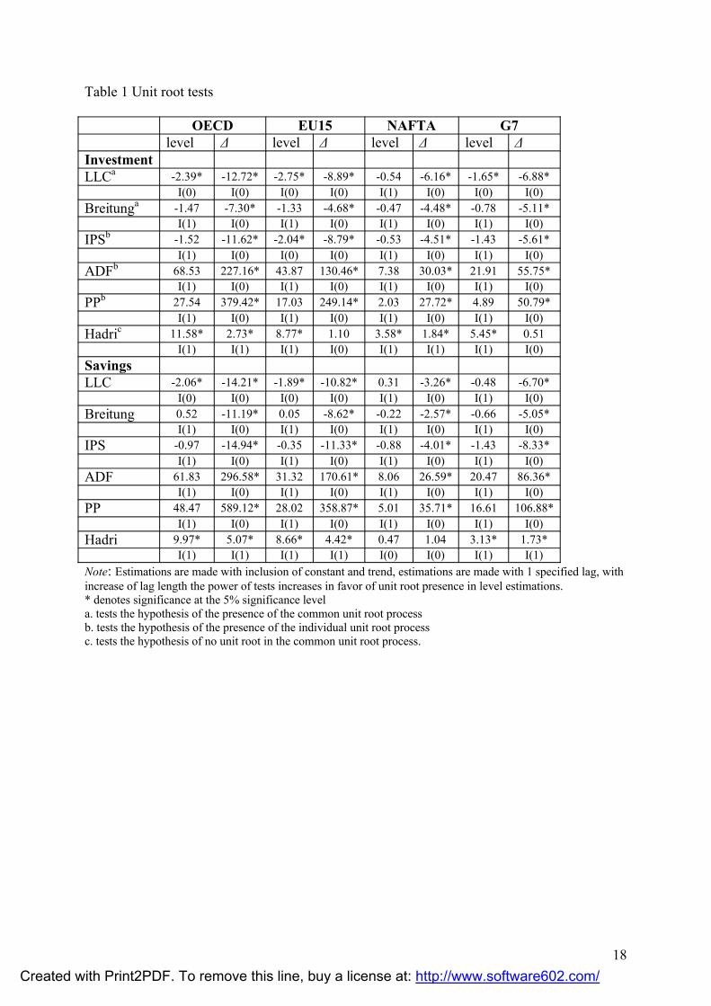
integration order of panel series. Six alternative unit root tests, the LLC, Breitung, IPS, ADF,

PP and Hadri tests, were employed in order to test for the presence of the unit root in panel

series. The LLC and the Breitung tests have a null hypothesis of the common unit root process

presence; the IPS, the ADF and the PP test for a presence of individual unit root process in

series; and finally, the Hadri test’s hypothesis is no unit root in the common unit root process.

The results of the unit root tests are presented in Table 1. The Investment and Savings series

in general for all four groups demonstrated the presence of the unit root in levels and no unit

root process in their first differences. However, the LLC test rejected the hypothesis of the

unit root presence in the levels of the OECD, EU15 and G7 investment series and in the

OECD and EU15 savings series. The IPS test rejected the presence of the individual unit root

process in the investment series for the EU15 group. However, Banerjee et al. (2004, 2005)

illustrated in their studies that if common sources of non-stationarity exist, tests such as the

LLC and IPS tend to over-reject the null hypothesis of non-stationarity in series. The LLC test

is based on the pooled regressions, therefore this test may not perform well compared to other

tests in the case where there is no need for pooling in series. Im et al. (2003) illustrated that

the LLC test tends to over- reject the null hypothesis in the case of models with serially

correlated errors. Breitung (2000) demonstrated that if individual specific trends are included

in pooled series the LLC and IPS tests may lose power. Therefore, based on the results of the

alternative unit root tests, it can be concluded that the Investment and Savings series for all

countries’ groups are generated by a non-stationary stochastic process.

The prerequisite of Hansen’s (1992) stability test is that the variables have to be non-

stationary. The results of the various panel root tests presented in Table 1 indicated the

existence of unit root in the considered variables. However, in order to acquire stronger

evidence of a unit root presence in unstable as well as in stable series, the panel unit root tests

proposed by Im et al. (2005) that allow for one and two structural shifts in series were applied.

The results for the LM unit root tests with structural shifts for OECD, EU15, NAFTA and G7

groups are reported in Tables 3-8. Both types of unit root tests with one and with two

structural shifts provide strong evidence of the unit root presence in the panel series of all four

considered groups of countries. The LM statistics for individual countries failed to reject the

stationarity hypothesis in many cases where one structural shift was allowed. However, the

tests in which two structural shifts were allowed, demonstrated stronger power to reject the

null hypothesis of series’ stationarity.


9

Based on the results of the panel unit root tests which are reported in Table 1 and in

Tables 3-8, investment and savings series are accepted as non-stationary, therefore Hansen’s

(1992) stability test can be applied. The results of the stability tests for all considered

countries are presented in Table 9. Only in the cases of Australia and Spain supF do the

statistics reject the null hypothesis of the stability of model parameters indicating the presence

of structural change in parameters, while in all other cases the model parameters appeared

stable. The meanF statistic, in the cases of Australia, Canada, Greece, Italy, the Netherlands,

New Zealand, Norway, Portugal, Spain, Switzerland, Turkey and the United States, reject the

hypothesis of cointegration in favor of the instability of the overall model in the considered

countries. The Lc statistic rejects the hypothesis of constant parameters in most cases where

the MeanF statistics found instability in the overall model. Countries where the stability of

parameters is rejected are: Australia, Canada, Greece, the Netherlands, New Zealand,

Norway, Portugal, Spain, Switzerland and the United States. The results of the stability test

moderately clearly divide the considered countries into two groups. The first group consists of

countries where no evidence was found for the presence of structural shifts, and these

countries are: Austria, Belgium, Denmark, Finland, France, Germany, Iceland, Ireland, Japan,

Korea, Luxemburg, Mexico, Sweden and the United Kingdom. In these countries none of the

applied tests provides evidence of instability. Another group consists of countries where at

least one of the stability tests detected the presence of sudden structural shifts in the model.

These countries are: Australia, Canada, Greece, Italy, the Netherlands, New Zealand, Norway,

Portugal, Spain, Switzerland, Turkey and the United States.

After investigating the stability properties of cointegrating vectors, the Westerlund (2006)

panel cointegration test with multiple structural breaks can be applied to the instable series.

Tables 10-13 present the results of the panel cointegration test allowing for multiple structural

shifts. The test was applied to the OECD, EU15, NAFTA and G7 groups, where only

countries which were found instable by the stability test (Table 9) were included. The test was

applied with the option to detect maximum five structural breaks. Panel A demonstrates the

results of the test in which structural shifts are allowed in constant, while Panel B illustrates

test results where structural shifts are allowed in both constant and trend of the regression.

The results indicate that the test detected different break locations for the estimated countries.

However, a tendency may be followed in results around some particular dates. For example,

there is a prevalence of breaks (in constant and in constant and trend) occurring in the period

1974-1977 for such countries as Canada, Greece, Italy, the Netherlands, New Zealand,

Norway, Portugal, Spain, Switzerland, Turkey. This can be explained by some historical facts


10

that occurred at that time and had long-rung negative effects on industrialized economies. The

years 1973 and 1974 were characterized by high oil world prices, the growth of which was

stimulated by the embargo proclaimed by the Organization of Arab Petroleum Exporting

Countries to the United States. As a result, the Organization of Petroleum Exporting Countries

started to raise world oil prices. The oil price shock in those years combined with the stock

market crash in the same period led to the suppression of the economic activities of many

developed countries.

The statistics of the LM panel test in all groups of countries differ for the case when

breaks are allowed only in level and for the case when breaks are allowed in level and in

trend. In the case when a break is allowed only in constant estimated statistics, for the OECD,

EU15, NAFTA and G7 groups, it does not reject the hypothesis of cointegration, while in

cases when a break is allowed in constant and trend, the LM statistics reject the null

hypothesis, providing no evidence for cointegration in all considered panels. Thus, it can be

concluded that the investment and savings variables in the panels with unstable models are

cointegrated only around a broken intercept.

The Pedroni (1999) and Kao (1999) panel cointegration tests were employed to series

after finding evidence of variables non-stationarity (Table 1). Table 2 presents the results of

the Pedroni (1999) and Kao (1999) panel cointegration tests. The panel cointegration tests are

applied to four groups: OECD, EU15, NAFTA and G7. Only two statistics out of seven in the

Pedroni test provided evidence of cointegration between investment and savings series in the

cases of the OECD and EU15 countries. However, in the case of NAFTA and G7 groups, the

Pedroni test did not provide any evidence of the presence of cointegrating relationships

between variables. The results of the Kao panel cointegration test demonstrate the evidence of

cointegration existence between investment and savings series in OECD, EU15 and G7

groups and the Kao test did not provide any evidence in favor of cointegration in the NAFTA

group. The Kao cointegration test is quite sensitive to the information criterion used and to lag

selection. For example, the test does not reject the hypothesis of no cointegration in the

OECD and EU15 groups, choosing maximum 4 and 5 lags based on AIC and HQIC. As a

result, it can be seen that there is fairly weak evidence in favor of the presence of

cointegrating relationships in the OECD and EU15 groups and no evidence was found for

cointegration in the NAFTA and G7 groups. Thus, there is not enough evidence to support the

existence of long-run relationships between savings and investments in developed countries.

The results of the Pedroni and the Kao cointegration tests for the panels of the OECD,

EU15, NAFTA and G7 series which are presented in Table 2 did not provide significant


11

evidence for cointegrating relationships between the investment and saving variables. At the

same time, the test for cointegration with multiple structural breaks detected the presence of

cointegration in unstable series around broken intercept. However, in order to have full

analysis of capital mobility in developed countries, it is necessary to test for cointegration in

panels where only stable countries are included. Therefore, Table 14 presents the results of

the Pedroni and the Kao panel cointegration tests, where OECD, EU15, NAFTA and G7

groups are divided into groups with unstable countries (U) and into groups with stable

countries (S). In the case of NAFTA, the Pedroni and the Kao panel tests could not be applied

to the subgroup of stable countries due to panel absence. In this group only one country,

Mexico, is included, therefore the Johansen cointegration test was applied to the Mexico case.

From results of Table 14 it can be seen that the division of the NAFTA and G7 groups into

stable and unstable countries did not change the results which were extracted from the full

sample in Table 2. Thus, in the NAFTA and G7 groups no evidence was found in favor of

cointegration among investment and savings variables. In the cases of the OECD and EU15

countries, again weak evidence was found in favor of cointegration among unstable series;

however, in the case of stable series, the Pedroni and Kao tests provided stronger evidence of

cointegration indicating that investment and savings variables are cointegrated with the panel

of stable countries in the OECD and EU15 groups.

Previous studies (for example, Coakley et al., 1996) suggest that cointegration

between investment and saving series exist irrespective of level of capital mobility, which is

the indication of current account solvency. Thus, the results of cointegration tests indicate on

current account insolvency in the NAFTA and G7 groups and on current account solvency in

stable countries of the OECD and EU15 countries, with weaker evidence in unstable

countries.

Kumar and Rao (2009) in their panel study on 13 OECD countries applying the

Pedroni (1999) cointegration test found some evidence of cointegration in series as well;

however, dividing the panel into pre- and post- Bretton Woods and pre- and post- Maastricht

sub-samples decreased the significance of test statistics providing less evidence in favor of

cointegration. Similar to the results of the present study, Narayan and Narayan (2010) in their

panel analysis of G7 countries applying the Pedroni (1999) cointegration test, did not find any

evidence of cointegration between investment and savings series. The authors concluded that

the absence of long-term relationships between variables indicates the highly mobility of

capital in G7 countries.


12

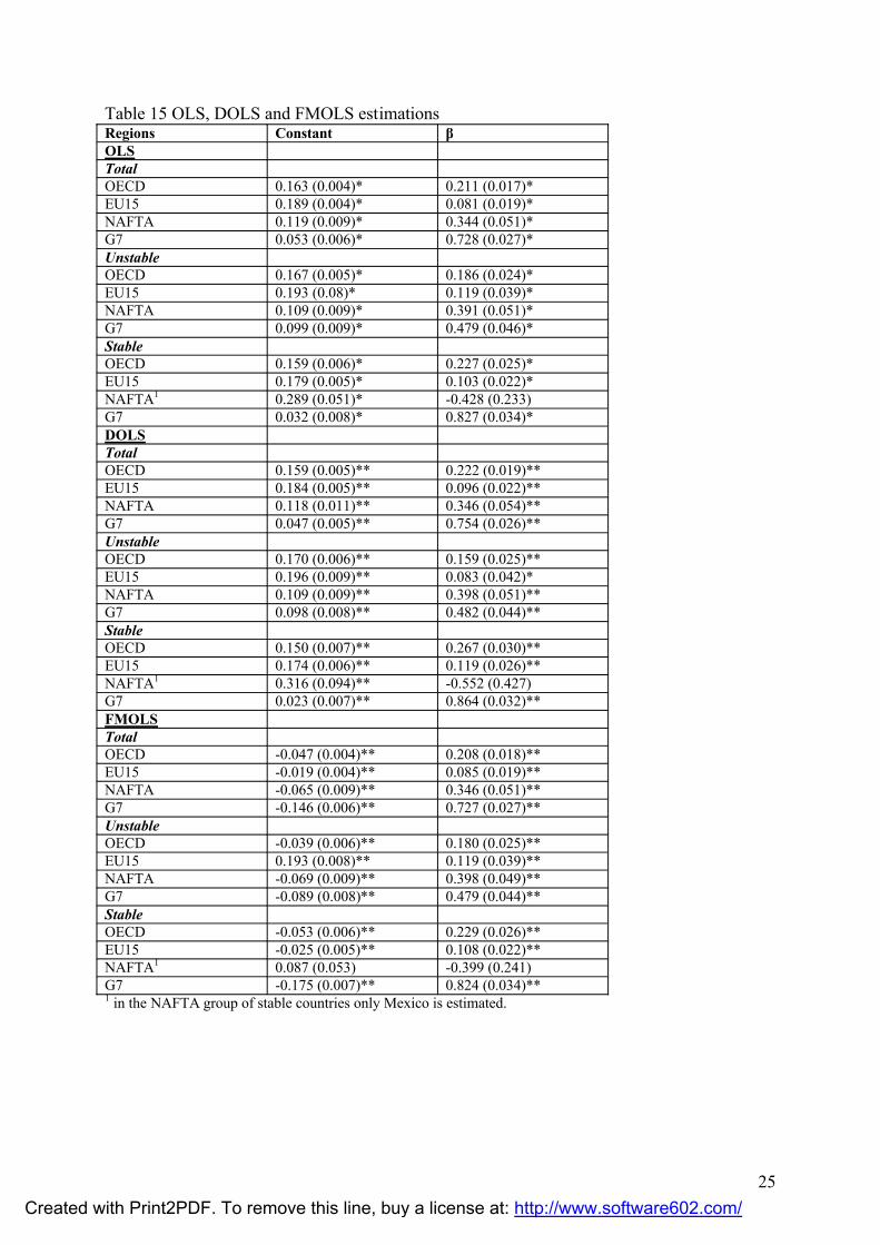
Finally, this study examines the saving retention coefficient β from Equation 1 by

employing least squares (OLS, DOLS and FMOLS) estimators. The results, presented in

Table 15, do not show significant difference in coefficient estimates when different least

squares estimators were employed. Saving retention coefficients are considered for all

considered groups of developed countries, dividing them in 3 different cases, total, unstable

and stable. The first case indicates coefficient estimates for panels where all countries of the

particular group are included. In the second case only unstable countries are included in

estimations, while in the last case, only stable countries are included.

In all cases, except for the NAFTA stable group, the saving retention coefficient was

found with the expected positive sign. The saving retention coefficient in the OECD group is

estimated at 0.2223, where the division of this group by unstable and stable countries did not

change its magnitude significantly. The saving retention coefficient for EU15 countries is

estimated even at a lower level than for OECD countries, 0.096 for the full sample, and 0.083

and 0.119 for the unstable and stable groups, respectively. These results contradict the

Feldstein-Horioka (1980) results, indicating capital mobility in OECD countries. Similar

results are found in Kollias et al. (2008) where the saving retention coefficient for EU15

1962-2002 period was found at the 0.148 level. The saving retention coefficient in the Kumar

and Rao (2009) panel study on 13 OECD countries was found to be very sensitive to the

choice of period and model. Thus, they found that the saving retention coefficient for the pre-

Bretton Woods period in the model with random effects is 0.742, while the estimation of

model with fixed effects for the post-Bretton Woods period generated a saving retention

coefficient at the level 0.266.

The coefficient estimates for NAFTA are 0.346 and 0.398 for total and unstable

panels, respectively, while in the case of stable countries the saving retention coefficient

appeared to be negative -0.552 in all three cases of coefficient estimates, OLS, DOLS and

FMOLS. The stable case of NAFTA includes only one country, Mexico. The negative

association between investment and savings was detected and explained in previous studies

on capital mobility (see, for example, Özmen [2007], Fouquau et al. [2008]). For example,

Westphal (1983) in his study provided theoretical explanation for the existence of negative

relations between investments and savings. Particularly, a high world interest rate leads

domestic interest rates to increase promoting by this growth in domestic savings and decline

in domestic investments. In the G7 group, however, saving retention coefficient estimates

3 Even though estimates of OLS, DOLS, and FMOLS do not differ significantly, in the saving-retention coefficient discussion, DOLS estimates are used.


13

differ from other estimates according to group division. Thus, the saving retention coefficient

is estimated at the level 0.754 in the full sample and at levels 0.482 and 0.864 in the unstable

and stable panels of G7 group. The results illustrate that the group of unstable countries in the

G7 group, which are Canada, Italy and the United States, have a saving retention coefficient

which indicates moderate capital mobility in these countries. The stable countries of the G7,

which are France, Germany, Japan and the United Kingdom, appeared to have low capital

mobility. Thus, only the extraction of the most developed countries from the OECD group

with stable economies appeared to fall in the Feldstein-Horioka puzzle.

The results illustrate that saving retention coefficient estimations are significant in

panel samples. The wider panel of developed countries is considered the more general results

are obtained. Therefore, the division of considered panels in groups with more common

characteristics provides different and more specific results.

4. Conclusion

This paper examined the validity of the Feldstein-Horioka puzzle for the panel sample of

OECD countries. The OECD countries were analyzed in more narrow groups as well, EU15,

NAFTA and G7, in order to compare the results of the analysis of developed countries when

they are combined in different panels. Recently developed econometric methods were applied

to annual series in order to investigate the cointegrating relationships of investment and

savings variables, taking into account the presence of structural shifts in the model when it

was relevant and to estimate the saving retention coefficient. To detect series where structural

shifts took place, the Hansen’s (1992) stability test was employed. As a result, 12 countries

out of 26 OECD countries were exposed as unstable countries. The Westerlund (2006)

cointegration test was applied to four groups of countries, OECD, EU15, NAFTA and G7,

where only unstable countries were included, allowing for maximum five breaks. As a result,

evidence of cointegration was found only in the presence of constant, while no evidence was

found when constant and trend are included. The Pedroni and Kao panel cointegration tests

did not provide any evidence of cointegration for the NAFTA and G7 panels when tests were

run for full samples and for sample divided into stable and unstable groups. In the case of the

OECD and EU15 countries, the Pedroni and Kao tests provided fairly weak evidence of

cointegration between investment and savings variables. However, when these panels were

divided into stable and unstable groups, tests for groups with stable countries with constant

inclusion provided much stronger evidence for cointegration presence than for full samples


14

and for samples with unstable countries indicating long-run relationships between investment

and savings in stable OECD and EU15 countries.

Finally, a saving retention coefficient was estimated for the OECD, EU15, NAFTA and

G7 groups and for their unstable and stable subgroups. DOLS estimations indicated the lowest

coefficient 0.096 for the EU15 group and the highest 0.784 for the G7 group. The division of

the full sample by stable and unstable groups did not change the results significantly except

for the G7 group, where the saving retention coefficient for the unstable group was estimated

at the 0.482 level, and for the group with the stable countries, the saving retention coefficient

increased to 0.864.

This study illustrates that the analysis of capital mobility in OECD developed countries is

sensitive to panel selection, OECD, EU15, NAFTA or G7. The presence of uncounted

structural shifts may lead to the underestimation of cointegration tests and saving retention

coefficients. The results of this study illustrate that the Feldstein-Horioka puzzle exists only in

the panel of G7 countries, while the extraction of unstable countries significantly decreases

the saving retention coefficient.

5. References

Adedeji, O. & Thornton, J. (2008). International capital mobility: Evidence from panel cointegration tests. Economics Letters, 99, 349-352.

Apergis, N., & Tsoumas, C. (2009). A survey on the Feldstein Horioka puzzle: What has been done and were we stand. Research in Economics. Forthcoming.

Argimon, I., & Roldan, J.M. (1994). Saving, investment and international capital mobility in EC countries. European Economic Review, 38, 59-67.

Banerjee, A. & Zanghieri, P. (2003). A new look at the Feldstein-Horioka puzzle using an integrated panel. CEPII Working Paper, 22.

Banerjee, A., Marcellino, M. & Osbat, C. (2004). Some Cautions on the Use of PanelMethods for Integrated Series of Macro-Economic Data. Econometrics Journal, 7, 322-340.

Banerjee, A., Marcellino, M. & Osbat, C. (2005). Testing for PPP: Should We Use Panel Methods? Empirical Economics, 30, 77-91.

Blanchard, O. & Giavazzi, F. (2002). Current account deficit in the Euro area: The end of the Feldstein-Horioka Puzzle? Brookings Papers on Economic Activity, 2, 147-186.

Breitung, J. (2000). The local power of some unit root tests for panel data. Advances inEconometrics, Volume 15: Nonstationary Panels, Panel Cointegration, and DynamicPanels, ed. B. H. Baltagi, 161–178. Amsterdam: JAY Press.

Breitung, J. (2000). The Local Power of Some Unit Root Tests for Panel Data. in B.Baltagi (ed.), Nonstationary Panels, Panel Cointegration, and Dynamic Panels, (Advances in Econometrics, 15), 161-178, Elsevier Science.

Caporale, G.M., Panopoulou, E., & Pittis, N. (2005). The Feldstein-Horioka puzzle revisited: a monte carlo study. Journal of International Money and Finance, 24, 1143-49.


15

Choi, I. (2001). Unit Root Tests for Panel Data. Journal of International Money and Finance,20, 249-272.

Coakley, J., & Kulasi, F. (1997). Cointegration of long run saving and investment. Economics Letters, 54, 1 – 6.

Coakley, J., Kulasi, F., & Smith, R. (1998). The Feldstein-Horioka puzzle and capital mobility: A review. International Journal of Finance and Economics, 3, 169-188.

Coakley, J., Kulasi, F., & Smith, R. (1996). Current account solvency and the Feldstein–Horioka puzzle. Economic Journal, 106, 620−627.

Corbin, A. (2001). Country specific effect in the Feldstein-Horioka paradox: a panel data analysis. Economics Letters, 72(3), 297-302.

Dooley, M., Frankel, J.A., & Mathieson, D.J. (1987). International capital mobility: what do saving-investment correlations tell us? International Monetary Fund Staff Papers, 34, 503 – 530.

Feldstein, M., & Horioka, C. (1980). Domestic saving and international capital flows. Economic Journal, 90, 314–329.

Fouquau, J., Hurlin, C., & Rabaud, I. (2008). The Feldstein-Horioka puzzle: A panel smooth transition regression approach. Economic Modelling, 25, 284-299.

Frankel, J. A. (1992). Measuring international capital mobility – A review. American Economic Review, 82, 197-202.

Georgopoulos, G. & Hejazi, W. (2009). The Feldstein–Horioka puzzle revisited: Is the home-bias much less? International Review of Economics & Finance, 18(2), 341-350.

Hadri, K. (2000). Testing for stationarity in heterogenous panel data. Econometrics Journal,3(2), 148-161.

Hansen, E. B. (1992). Tests for parameter instability in regressions with I(1) process. Journal of Business and Economic Statistics,10(3), 321-335.

Herwartz, H. & Xu, F. (2010). A functional coefficient model view of the Feldstein–Horioka puzzle. Journal of International Money and Finance, 29(1), 37-54.

Ho, T.W. (2002). The Feldstein-Horioka puzzle revisited. Journal of International Money and Finance, 21, 555-564.

Jansen, W.J. (1996). Estimating saving-investment correlations: evidence for OECD countries based on an error correction model. Journal of International Money and Finance, 15, 749-81.

Im, K.S., Lee, J. & Tieslau, M. (2005). Panel LM unit-root tests with level shifts. Oxford Bulletin of Econometrics and Statistics 67(3), 393–419.

Im, K.S., Pesaran, M.H. & Shin, Y. (2003). Testing for unit root in heterogenous panels. Journal of Econometrics, 115(1), 53-74.

Kao, C. (1999). Spurious regression and residual-based tests for cointegration in panel data.Journal of Econometrics, 90, 1–44.

Kao, C. & Chiang, M.H. (2001). On the Estimation and Inference of a Cointegrated Regression in Panel Data. Advances in Econometrics, 15, 179–222.

Kejriwal, M. (2008). Cointegration with structural breaks: An application to the Feldstein-Horioka puzzle. Studies in Nonlinear Dynamics and Econometrics, 12(1), article 3.

Kollias, C., Mylonidis, N. & Paleologou, S.M. (2008). International Review of Economics and Finance, 17, 380-387.

Kumar, S. & Rao, B.B. (2009). A Time Series Approach to the Feldstein-Horioka Puzzle with Panel Data from the OECD Countries. MPRA Paper, University Library of Munich, Germany.

Kwiatkowski, D., Phillips, P.C.B, Schmidt, P. & Shin, Y. (1992). Testing the null hypothesis of stationarity against the alternative of a unit root: How sure are we that economic time series have a unit root? Journal of Econometrics, 44, 159-178.


16

Lee, J. & Strazicich, M. (2001). Break point estimation and spurious rejections with endogenous unit root tests. Oxford Bulletin of Economics and Statistics, 63, 535–558.

Lee, J. & Strazicich, M. (2003). Minimum Lagrange multiplier unit root test with twostructural breaks. Review of Economics and Statistics, 85, 1082–1089.

Lee, J. & Strazicich, M.C. (2004). Minimum LM unit root test with one structural break. Working Papers 04-17, Department of Economics, Appalachian State University.

Levin, A., Lin, C.F. & Chu, C.S.J. (2002). Unit root tests in panel data: Asymptotic and finite-sample properties. Journal of Econometric, 108(1), 1-24.

Maddala, G.S. & Wu, S. (1999). A comparative study of unit root tests with panel data and a new simple test. Oxford Bulletin of Economics and Statistics, 61, 631–652.

Mastroyiannis, A. (2007). Current account dynamics and the Feldstein and Horioka puzzle: the case of Greece. The European Journal of Comparative Economics, 4(1), 91-99.

McCoskey, S. & Kao, C. (1998). A residual-based test of the null of cointegration in panel data. Econometric Reviews, 17(1), 57-84.

Miller, S.M. (1988). Are saving and investment cointegrated? Economics Letters, 27, 31 – 34. Murphy, R.G. (1984). Capital mobility and the relationship between saving and investment in

OECD countries. Journal of International Money and Finance, 3, 327-342. Narayan, P.K. & Narayan, S. (2010). Testing for capital mobility: New evidence from a panel

of G7 countries. Research in International Business and Finance, 24(1), 15-23.Obstfeld, M., & Rogoff, K. (2000). Perspectives on OECD economic integration: Implications

for U.S. Current Account Adjustment. UC Berkeley: Center for International andDevelopment Economics Research. Retrieved from: http://escholarship.org/uc/item/16z3s2s2

Ozmen, E. & Parmaksız, K. (2003). Policy regime change and the Feldstein-Horioka puzzle: the UK evidence. Journal of Policy Modeling, 25, 137-149.

Ozmen, E. (2007). Financial development, exchange rate regimes and the Feldstein-Horioka puzzle: evidence from the MENA region. Applied Economics, 39(9), 1133-1138.

Pedroni, P. (1999). Critical values for cointegration tests in heterogeneous panels withmultiple regressors. Oxford Bulletin of Economics and Statistics November (Special Issue), 653–669.

Penati, A., & Dooley, M. (1984). Current account imbalances and capital formation in industrial countries, 1949 – 1981. International Monetary Fund Staff Papers, 31, 1 –24.

Phillips, P.C.B., & Hansen, B.E. (1990). Statistical Inference in Instrumental Variables Regression with I(1) Processes. Review of Economic Studies, 57, 99-125.

Rao, B.B., Tamazian, A. & Kumar, S. (2010). Systems GMM estimates of the Feldstein–Horioka puzzle for the OECD countries and tests for structural breaks. Economic Modelling, forthcoming.

Schmidt, P. & Phillips, P. C. B. (1992). Testing for a unit root in the presence of deterministic trends. Oxford Bulletin of Economics and Statistics, 54, 257-287.

Sinha, T., & Sinha, D. (2004). The mother of all puzzles would not go away. Economic Letters, 82, 259-267.

Telatar, E., Telatar, F., & Bolatoglu, N. (2007). A regime switching approach to the Feldstein-Horioka puzzle: Evidence from some European countries. Journal of Policy Modeling,29(3), 523-533.

Tsung-wu Ho, T.W. (2002). The Feldstein–Horioka puzzle revisited. Journal of International Money and Finance, 21(4), 555-564.

Vasudeva Murthy, N. R. (2009). The Feldstein–Horioka puzzle in Latin American and Caribbean countries: a panel cointegration analysis. Journal of Economics and Finance, 33(2), 176-188.


17

Westerlund, J. (2006). Testing for Panel Cointegration with Multiple Structural Breaks.Oxford Bulletin of Economics and Statistics, 68(1), 101-132.

Westphal, U. (1983). Comments on “domestic saving and international capital flows in thelong-run and the short-run” by M. Feldstein. European Economic Review, 21, 157-159.


18

Table 1 Unit root tests

OECD EU15 NAFTA G7level Δ level Δ level Δ level Δ

InvestmentLLCa -2.39* -12.72* -2.75* -8.89* -0.54 -6.16* -1.65* -6.88*

I(0) I(0) I(0) I(0) I(1) I(0) I(0) I(0)Breitunga -1.47 -7.30* -1.33 -4.68* -0.47 -4.48* -0.78 -5.11*

I(1) I(0) I(1) I(0) I(1) I(0) I(1) I(0)IPSb -1.52 -11.62* -2.04* -8.79* -0.53 -4.51* -1.43 -5.61*

I(1) I(0) I(0) I(0) I(1) I(0) I(1) I(0)ADFb 68.53 227.16* 43.87 130.46* 7.38 30.03* 21.91 55.75*

I(1) I(0) I(1) I(0) I(1) I(0) I(1) I(0)PPb 27.54 379.42* 17.03 249.14* 2.03 27.72* 4.89 50.79*

I(1) I(0) I(1) I(0) I(1) I(0) I(1) I(0)Hadric 11.58* 2.73* 8.77* 1.10 3.58* 1.84* 5.45* 0.51

I(1) I(1) I(1) I(0) I(1) I(1) I(1) I(0)SavingsLLC -2.06* -14.21* -1.89* -10.82* 0.31 -3.26* -0.48 -6.70*

I(0) I(0) I(0) I(0) I(1) I(0) I(1) I(0)Breitung 0.52 -11.19* 0.05 -8.62* -0.22 -2.57* -0.66 -5.05*

I(1) I(0) I(1) I(0) I(1) I(0) I(1) I(0)IPS -0.97 -14.94* -0.35 -11.33* -0.88 -4.01* -1.43 -8.33*

I(1) I(0) I(1) I(0) I(1) I(0) I(1) I(0)ADF 61.83 296.58* 31.32 170.61* 8.06 26.59* 20.47 86.36*

I(1) I(0) I(1) I(0) I(1) I(0) I(1) I(0)PP 48.47 589.12* 28.02 358.87* 5.01 35.71* 16.61 106.88*

I(1) I(0) I(1) I(0) I(1) I(0) I(1) I(0)Hadri 9.97* 5.07* 8.66* 4.42* 0.47 1.04 3.13* 1.73*

I(1) I(1) I(1) I(1) I(0) I(0) I(1) I(1)Note: Estimations are made with inclusion of constant and trend, estimations are made with 1 specified lag, with increase of lag length the power of tests increases in favor of unit root presence in level estimations. * denotes significance at the 5% significance levela. tests the hypothesis of the presence of the common unit root processb. tests the hypothesis of the presence of the individual unit root processc. tests the hypothesis of no unit root in the common unit root process.


19

Table 2 Panel cointegration tests

OECD EU15 NAFTA G7c c&t c c&t c C&t c c&t

PedroniPanel v-Statistic 1.70* -1.37 1.02 -0.69 0.42 -0.84 0.56 -0.22Panel rho-Statistic -1.28 0.14 -1.24 -0.12 -0.50 0.11 0.14 1.18Panel PP-Statistic -1.06 -0.43 -1.58 -0.91 -0.13 0.07 0.22 1.15Panel ADF-Statistic -2.32** -2.65** -2.69** -2.91** -0.14 0.11 -0.80 0.46Group rho-Statistic 1.07 2.19 0.59 1.42 0.82 1.28 1.43 2.05Group PP-Statistic 0.26 1.16 -0.89 0.27 1.13 1.18 1.05 1.92Group ADF-Statistic -1.52 -1.67* -2.81** -2.74** 0.92 0.38 -0.45 0.99

KaoADF -4.09** -4.09** -1.23 -1.96*

Note: The critical values are based on Pedroni (2004). Hypothesis for Pedroni cointegration test: No cointegration. ** and * reject hypothesis of no cointegration at 1% and 5% level of significance.Lag selection is based on the SIC with maximum 3 lags.

Table 3. Panel unit root test with one structural break - OECDCountry Investment Saving

LM Break Lag LM Break LagAustralia -2.799 1999 3 -4.671** 1993 1Austria -3.321 1997 0 -4.482* 1994 2Belgium -3.390 1989 0 -4.173 1983 0Canada -2.688 1990 0 -3.059 1998 2Denmark -4.027 1978 3 -4.048 1984 2Finland -3.788 1990 1 -3.238 1988 1France -4.977* 1994 2 -4.730** 1985 3Germany -5.022** 1993 1 -3.028 1992 3Greece -4.141 1997 1 -3.135 1990 0Iceland -3.770 1994 1 -3.803 1985 0Ireland -3.422 1976 3 -3.600 1992 2Italy -3.359 2001 1 -4.573** 1983 2Japan -2.629 1987 1 -3.514 1992 3Korea -4.666** 1993 1 -3.981 1983 1Luxemburg -4.897** 1985 0 -3.503 1985 1Mexico -4.584** 1984 1 -3.159 1986 3Netherlands -4.049 1987 2 -3.415 1986 3New Zealand -6.061*** 1990 2 -6.100*** 1980 3Norway -4.675** 1988 2 -2.961 1993 0Portugal -3.841 1996 1 -6.597*** 1980 3Spain -4.018 1980 1 -4.036 1976 3Sweden -3.487 1990 1 -3.771 1996 1Switzerland -3.799 1983 3 -3.041 1990 1Turkey -4.251* 1986 2 -3.755 1980 2UK -5.852*** 1983 1 -4.707** 1981 2US -3.961 1996 1 -3.003 1976 3MinLM -3.961 1996 1 -3.003 1976 3LM statistic -17.469*** -16.512***Notes: For the one break case, the 1%, 5% and 10% critical values for the panel LM test with a break are −2.326, −1.645 and −1.282, respectively. The 1%, 5% and 10% critical values for the minimum LM test with one break are −5.11, −4.50 and −4.21, respectively (Lee and Strazicich (2003)). The 1%, 5% and 10% critical values for the minimum LM test with two breaks are −5.823, −5.286 and −4.989, respectively (Lee and Strazicich [2001,2003]). *denotes significance at the 1% level


20

Table 4. Panel unit root test with two structural breaks - OECDInvestment Saving

LM Break1 Break2

Lag LM Break1 Break2

Lag

Australia -4.169 1979 1998 1 -5.468** 1980 1993 2Austria -5.875*** 1982 1993 0 -5.863*** 1981 1998 2Belgium -4.547 1987 2000 3 -5.557** 1977 2002 0Canada -4.620 1980 1997 1 -4.593 1980 1997 3Denmark -5.352** 1983 1991 3 -4.985* 1981 1997 3Finland -5.290** 1979 1991 3 -4.434 1982 1993 1France -7.105*** 1984 1994 2 -6.761*** 1978 1993 3Germany -6.076*** 1981 1999 3 -4.391 1975 1993 1Greece -6.441*** 1983 1998 3 -4.739 1975 1992 1Iceland -6.129*** 1976 1996 2 -4.921 1980 1996 1Ireland -7.032*** 1979 1993 3 -7.229*** 1980 2000 3Italy -4.577 1983 1999 3 -5.193* 1975 1992 1Japan -7.521*** 1987 1996 3 -5.943*** 1988 1999 3Korea -5.721** 1975 1997 1 -5.871*** 1975 1991 2Luxemburg -6.079*** 1984 1990 2 -4.777 1975 1985 1Mexico -6.394*** 1987 1984 2 -4.411 1982 1995 0Netherlands -5.673** 1975 2001 2 -4.277 1986 1999 3New Zealand -7.846*** 1980 1990 2 -7.044*** 1975 1980 3Norway -5.827*** 1978 1988 2 -6.136*** 1977 1996 1Portugal -5.545** 1989 2001 1 -7.974*** 1980 1984 3Spain -4.610 1984 1995 1 -4.614 1990 1999 3Sweden -6.068*** 1982 1991 1 -5.514*** 1981 1992 1Switzerland -5.542** 1981 1990 3 -4.615 1978 2001 1Turkey -6.481*** 1980 1997 3 -8.360*** 1978 1986 3UK -7.394*** 1983 1997 1 -5.799** 1976 1986 3US -5.455** 1986 1996 1 -4.564 1980 1992 3MinLM -5.455** 1986 1996 -4.564 1980 1992LM statistic -36.792*** -29.804**** denotes significance at the 1% level

Table 5. Panel unit root test with one structural break – EU15Country Investment Saving

LM Break Lag LM Break LagAustria -3.763 1998 0 -3.637 1994 1Belgium -3.158 1979 1 -4.409* 1988 0Denmark -5.003** 1988 3 -3.690 1995 3Finland -4.555* 1990 1 -3.336 1988 1France -5.748*** 1995 2 -4.324* 1985 3Germany -4.796** 1993 1 -2.587 1989 3Greece -4.186 1988 1 -3.300 1990 0Ireland -3.587 1976 3 -3.738 1995 0Italy -3.396 1992 1 -5.104** 1983 2Luxemburg -5.301*** 1990 2 -3.408 1985 1Netherlands -3.522 1985 1 -2.818 1986 3Portugal -3.851 1996 1 -6.013** 1980 3Spain -4.742** 1979 1 -4.195 1980 3Sweden -3.471 1990 1 -3.741 1990 1UK -6.283*** 1983 1 -5.523*** 1981 2MinLM -6.283*** 1983 1 -5.523*** 1981 2LM statistic -15.108*** -12.892**** denotes significance at the 1% level


21

Table 6. Panel unit root test with two structural breaks – EU15Investment Saving

LM Break1 Break2

Lag LM Break1 Break2

Lag

Austria -5.397** 1982 1996 0 -5.424** 1981 2001 2Belgium -3.712 1979 1989 1 -6.648*** 1988 2001 2Denmark -5.946*** 1978 1987 3 -5.301** 1986 1997 3Finland -5.464** 1980 1991 1 -4.913 1982 1993 1France -6.660*** 1978 1995 2 -5.284* 1982 1993 3Germany -5.700** 1993 2001 1 -4.431 1986 1998 3Greece -6.072*** 1983 2000 3 -4.897 1975 1992 1Ireland -6.892*** 1979 1993 3 -7.321*** 1979 2000 3Italy -4.988* 1983 2000 1 -5.501** 1983 1997 3Luxemburg -6.870*** 1984 1990 3 -4.659 1975 1985 1Netherlands -5.243* 1975 1999 2 -3.542 1986 1995 3Portugal -5.450** 1989 2001 1 -8.549*** 1978 1987 3Spain -5.241* 1984 1995 1 -5.395** 1988 2002 3Sweden -4.806 1986 1999 1 -5.354** 1981 1992 1UK -7.419*** 1983 2003 1 -6.066*** 1981 1986 2MinLM -7.419*** 1983 2003 1 -6.066*** 1981 1986 2LM statistic -23.757*** -22.755***

* denotes significance at the 1% level

Table 7. Panel unit root test with one structural break – NAFTA and G7Country Investment Saving

LM Break Lag LM Break LagNAFTACanada -3.786 1995 2 -3.053 1976 1Mexico -4.408* 1984 1 -5.200*** 1986 3US -4.762** 1997 1 -3.893 1980 3MinLM -4.762** 1997 1 -3.893 1980 3LM statistic -6.668*** -5.921***

G7Canada -2.972 1991 1 -3.876 1997 3France -3.394 1996 2 -5.211*** 1986 3Germany -4.067 1993 3 -2.862 1975 1Italy -4.647** 1999 1 -4.789** 1983 2Japan -3.789 1988 3 -2.926 1992 1UK -4.482 1982 1 -5.281*** 1983 2US -3.968 1993 1 -3.082 1975 3MinLM -3.968 1993 1 -3.082 1975 3LM statistic -8.382*** -8.900**** denotes significance at the 1% level


22

Table 8. Panel unit root test with two structural breaks – NAFTA and G7Investment Saving

LM Break1 Break2 Lag LM Break1 Break2 LagNAFTACanada -5.924*** 1985 2000 2 -4.285 1980 1998 1Mexico -5.539** 1982 1993 2 -5.545** 1988 2002 3US -5.423** 1985 1994 1 -4.050 1980 1993 3MinLM -5.423** 1985 1994 1 -4.050 1980 1993 3LM statistic -10.461*** -7.542***G7Canada -5.822*** 1980 1999 3 -5.069* 1982 1997 3Germany -5.153* 1980 2002 2 -6.691*** 1980 1993 3France -5.273* 1992 1999 3 -4.744 1980 1994 1Italy -4.817 1992 2000 3 -6.713*** 1979 1992 2Japan -5.459** 1986 1996 3 -4.905 1987 1999 1UK -5.867*** 1983 1997 1 -6.063*** 1981 1986 2US -5.828*** 1987 1996 1 -5.007* 1982 1999 0MinLM -5.828*** 1987 1996 1 -5.007* 1982 1999 0LM statistic -15.130*** -15.779**** denotes significance at the 1% level

Table 9. Stability tests in cointegrated relationsCountry SupF MeanF Lc b1

test p-value Test p-value test p-valueAustralia 2.145 0.01 102.41 0.01 901.61 0.01 -1.70 (0.37)Austria 0.27 0.20 2.26 0.20 3.53 0.20 0.07(0.32)Belgium 0.058 0.20 0.65 0.20 3.52 0.20 0.62 (0.37)Canada 0.34 0.20 5.79 0.07 15.83 0.04 -0.48 (0.18)Denmark 0.16 0.20 1.29 0.20 3.45 0.20 0.66 (0.39)Finland 0.11 0.20 2.41 0.20 7.10 0.20 0.29 (0.19)France 0.02 0.20 1.53 0.20 9.51 0.20 1.71 (1.23)Germany 0.23 0.20 3.76 0.20 11.09 0.20 0.78 (0.21)Greece 0.15 0.20 8.14 0.01 27.07 0.01 0.78 (0.10)Iceland 0.33 0.20 2.23 0.20 5.20 0.20 0.79 (0.86)Ireland 0.09 0.20 1.11 0.20 2.89 0.20 -0.17 (0.56)Italy 0.45 0.13 5.42 0.09 8.54 0.20 -0.12 (0.58)Japan 0.09 0.20 1.39 0.20 3.29 0.20 1.57 (0.52)Korea 0.05 0.20 0.81 0.20 1.91 0.20 2.15 (1.47)Luxemburg 0.17 0.20 1.99 0.20 4.43 0.20 0.39 (0.09)Mexico 0.09 0.20 1.63 0.20 3.62 0.20 -0.89 (0.71)Netherlands 0.35 0.20 9.05 0.01 67.52 0.01 0.96 (0.15)New Zealand 0.28 0.20 6.45 0.04 34.04 0.01 -0.07 (0.43)Norway 0.07 0.20 3.97 0.20 19.97 0.01 -1.02 (0.45)Portugal 0.46 0.13 14.46 0.01 45.48 0.01 -0.48 (0.44)Spain 0.89 0.01 12.19 0.01 55.82 0.01 0.18 (0.67)Sweden 0.09 0.20 4.02 0.20 12.26 0.15 0.24 (0.14)Switzerland 0.40 0.17 5.47 0.08 24.43 0.01 0.62 (0.23)Turkey 0.49 0.12 5.97 0.06 12.84 0.12 0.57 (0.15)UK 0.36 0.20 3.27 0.20 5.64 0.20 -0.31 (0.38)US 0.81 0.20 30.60 0.01 297.47 0.01 -0.12 (0.38)


23

Table10. Estimated structural breaks using the approach of Westerlund (2006). OECDPanel A breaks in constantCountry Breaks DateAustralia 3 1979 1996 2003Canada 4 1986 1991 1996 2003Greece 1 1997Italy 5 1974 1981 1987 1992 1999Netherlands 1 1974New Zealand 3 1975 1994 2002Norway 2 1989 1994Portugal 5 1974 1983 1988 1996 2002Spain 4 1977 1987 1998 2003Switzerland 1 1985Turkey 1 2003US 1 1997Lm 2.711Panel B breaks in constant and trendCountry Breaks DateAustralia 4 1979 1987 1993 1999Canada 5 1974 1983 1989 1996 2001Greece 3 1976 1983 2001Italy 5 1975 1981 1987 1992 2001Netherlands 5 1976 1984 1883 1998 2003New Zealand 5 1974 1980 1990 1995 2002Norway 4 1977 1989 1996 2002Portugal 2 1983 1997Spain 4 1976 1983 1990 1995Switzerland 3 1975 1991 2000Turkey 3 1977 1989 2000US 4 1980 1985 1992 2003Lm 13.919No breaksLm 1.521Lm (C) 9.606Lm (C + T) 7.742

Table 11. Estimated structural breaks using the approach of Westerlund (2006). EU15Panel A breaks in constantCountry Breaks DateGreece 1997Italy 1974 1981 1987 1992 1999Netherlands 1974Portugal 1974 1983 1988 1996 2002Spain 1977 1987 1998 2003Lm 1.989Panel B breaks in constant and trendCountry Breaks DateGreece 1976 1983 2001Italy 1975 1981 1987 1992 2001Netherlands 1976 1984 1993 1998 2003Portugal 1983 1997Spain 1976 1983 1990 1995Lm 7.338No breaksLm 1.207Lm (C) 4.864Lm (C + T) 4.345


24

Table12. Estimated structural breaks using the approach of Westerlund (2006). NAFTA Panel A breaks in constantCountry Breaks DateCanada 1986 1991 1996 2003US 1997Lm 1.142Panel B breaks in constant and trendCountry Breaks DateCanada 1974 1983 1989 1996 2001US 1980 1985 1992 2003Lm 7.571No breaksLm 0.935Lm (C) 3.853Lm (C + T) 4.626

Table13. Estimated structural breaks using the approach of Westerlund (2006). G7 Panel A breaks in constantCountry Breaks DateCanada 1986 1991 1996 2003Italy 1974 1981 1987 1992 1999US 1997Lm 1.466Panel B breaks in constant and trendCountry Breaks DateCanada 1974 1983 1989 1996 2001Italy 1975 1981 1987 1992 2001US 1980 1985 1992 2003Lm 8.140No breaksLm 0.586Lm (C) 4.858Lm (C + T) 6.186

Table 14 Panel cointegration testsOECD EU15 NAFTA G7

c c&t c c&t c c&t c c&t c c&t c c&t c c&t c c&tPedroni U S U S U S U S

Panel v-Statistic 0.89 -0.11 1.45* -1.49 -0.12 -1.23 1.58* 0.30 0.13 -0.27

- --0.09 -0.85 0.93 0.69

Panel rho-Statistic -0.12 0.13 -1.55* 0.08 -0.58 0.35 -1.15 -0.55 0.54 0.91

- -0.49 1.13 -0.34 0.46

Panel PP-Statistic -0.02 -0.61 -1.30* -0.14 -0.92 -0.48** -1.29* -0.86 0.94 0.92

- -0.65 1.02 -0.34 0.55

Panel ADF-Statistic -0.28 -2.08** -2.68** -1.79* -1.73* -2.30 -2.07** -1.84* 0.61 -0.03

- --0.11 -0.25 -1.00 0.73

Group rho-Statistic 1.16 1.66 0.38 1.45 0.57 1.03 0.32 1.01 1.19 1.39

- -1.33 1.73 0.74 1.21

Group PP-Statistic 0.58 0.68 -0.19 0.95 -0.96 -0.22 -0.42 0.48 1.58 1.38

- -1.14 1.61 0.39 1.15

Group ADF-Statistic -0.34 -1.40* -1.77* -0.97 -2.26** -2.64** -1.85* -1.49* 1.17 0.19

- -0.35 0.09 -0.90 1.23

Johansen 12.94 15.99KaoADF -1.82* -3.77** -2.54** -3.91** -0.64 - -1.46* -1.11Note: The critical values are based on Pedroni (2004). Hypothesis for Pedroni cointegration test: No cointegration. ** and * reject hypothesis of no cointegration at 1% and 5% level of significance. Lag selection is based on the SIC with maximum 3 lags.


25

Table 15 OLS, DOLS and FMOLS estimationsRegions Constant βOLSTotalOECD 0.163 (0.004)* 0.211 (0.017)*EU15 0.189 (0.004)* 0.081 (0.019)*NAFTA 0.119 (0.009)* 0.344 (0.051)*G7 0.053 (0.006)* 0.728 (0.027)*UnstableOECD 0.167 (0.005)* 0.186 (0.024)*EU15 0.193 (0.08)* 0.119 (0.039)*NAFTA 0.109 (0.009)* 0.391 (0.051)*G7 0.099 (0.009)* 0.479 (0.046)*StableOECD 0.159 (0.006)* 0.227 (0.025)*EU15 0.179 (0.005)* 0.103 (0.022)*NAFTA1 0.289 (0.051)* -0.428 (0.233)G7 0.032 (0.008)* 0.827 (0.034)*DOLSTotalOECD 0.159 (0.005)** 0.222 (0.019)**EU15 0.184 (0.005)** 0.096 (0.022)**NAFTA 0.118 (0.011)** 0.346 (0.054)**G7 0.047 (0.005)** 0.754 (0.026)**UnstableOECD 0.170 (0.006)** 0.159 (0.025)**EU15 0.196 (0.009)** 0.083 (0.042)*NAFTA 0.109 (0.009)** 0.398 (0.051)**G7 0.098 (0.008)** 0.482 (0.044)**StableOECD 0.150 (0.007)** 0.267 (0.030)**EU15 0.174 (0.006)** 0.119 (0.026)**NAFTA1 0.316 (0.094)** -0.552 (0.427)G7 0.023 (0.007)** 0.864 (0.032)**FMOLSTotalOECD -0.047 (0.004)** 0.208 (0.018)**EU15 -0.019 (0.004)** 0.085 (0.019)**NAFTA -0.065 (0.009)** 0.346 (0.051)**G7 -0.146 (0.006)** 0.727 (0.027)**UnstableOECD -0.039 (0.006)** 0.180 (0.025)**EU15 0.193 (0.008)** 0.119 (0.039)**NAFTA -0.069 (0.009)** 0.398 (0.049)**G7 -0.089 (0.008)** 0.479 (0.044)**StableOECD -0.053 (0.006)** 0.229 (0.026)**EU15 -0.025 (0.005)** 0.108 (0.022)**NAFTA1 0.087 (0.053) -0.399 (0.241)G7 -0.175 (0.007)** 0.824 (0.034)**1 in the NAFTA group of stable countries only Mexico is estimated.


the feldstein horioka puzzle by groups of oecd members: the

Documents