a fully integrated environment for time-dependent data analysis
TRANSCRIPT

A FULLY INTEGRATED ENVIRONMENTFOR TIME-DEPENDENT DATA ANALYSIS

Version 1.4
July 2007First editionIntended for use with Mathematica 6 or higher
Software and manual: Yu He, John Novak, Darren GlosemeyerProduct manager: Nirmal MalapakaProject manager: Nirmal MalapakaEditor: Jan ProgenSoftware quality assurance: Cindie StraterDocument quality assurance: Rebecca Bigelow and Jan ProjenGraphic design: Jeremy Davis and Megan Gillette
Published by Wolfram Research, Inc., 100 Trade Center Drive, Champaign, Illinois 61820-7237, USA phone: +1-217-398-0700; fax: +1-217-398-0747; email: [email protected]; web: www.wolfram.com
Copyright © 2007 Wolfram Research, Inc.
All rights reserved. No part of this documentation may be reproduced, stored in a retrieval system, or transmitted, in any form or by any means,electronic, mechanical, photocopying, recording, or otherwise, without the prior written permission of Wolfram Research, Inc.
Wolfram Research, Inc. is the holder of the copyright to the Time Series software system described in this document, including, without limitation, suchaspects of the system as its code, structure, sequence, organization, “look and feel”, programming language, and compilation of command names. Useof the system unless pursuant to the terms of a license granted by Wolfram Research, Inc. or as otherwise authorized by law is an infringement of thecopyright.
Wolfram Research, Inc. makes no representations, express or implied, with respect to this documentation or the software it describes, including,without limitation, any implied warranties of merchantability, interoperability, or fitness for a particular purpose, all of which are expresslydisclaimed. Users should be aware that included in the terms and conditions under which Wolfram Research is willing to license Time Series is aprovision that Wolfram Research and its distribution licensees, distributors, and dealers shall in no event be liable for any indirect, incidental,or consequential damages, and that liability for direct damages shall be limited to the amount of the purchase price paid for Time Series.
In addition to the foregoing, users should recognize that all complex software systems and their documentation contain errors and omissions.Wolfram Research shall not be responsible under any circumstances for providing information on or corrections to errors and omissionsdiscovered at any time in this document or the software it describes, whether or not they are aware of the errors or omissions. WolframResearch does not recommend the use of the software described in this document for applications in which errors or omissions could threatenlife, injury, or significant loss.
Mathematica is a registered trademark of Wolfram Research, Inc. All other trademarks are the property of their respective owners. Mathematica is notassociated with Mathematica Policy Research, Inc. or MathTech, Inc.

Table of ContentsGetting Started...............................................................................................................................................1
About Time Series....................................................................................................................................1
Part 1. User’s Guide to Time Series1.1 Introduction..............................................................................................................................................4
1.2 Stationary Time Series Models.............................................................................................................8
1.2.1 Autoregressive Moving Average Models.......................................................................................8
1.2.2 Stationarity......................................................................................................................................10
1.2.3 Covariance and Correlation Functions...........................................................................................15
1.2.4 Partial Correlation Functions..........................................................................................................20
1.2.5 Multivariate ARMA Models............................................................................................................22
1.3 Nonstationary and Seasonal Models..................................................................................................30
1.3.1 ARIMA Process................................................................................................................................30
1.3.2 Seasonal ARIMA Process.................................................................................................................31
1.4 Preparing Data for Modeling................................................................................................................37
1.4.1 Plotting the Data............................................................................................................................37
1.4.2 Generating Time Series...................................................................................................................42
1.4.3 Transformation of Data..................................................................................................................45
1.5 Estimation of Correlation Function and Model Identification......................................................53
1.5.1 Estimation of Covariance and Correlation Functions...................................................................53
1.5.2 The Asymptotic Distribution of the Sample Correlation Function...............................................57
1.5.3 The Sample Partial Correlation Function.......................................................................................61
1.5.4 Model Identification.......................................................................................................................62
1.5.5 Order Selection for Multivariate Series.........................................................................................65
1.6 Parameter Estimation and Diagnostic Checking..............................................................................68
1.6.1 Parameter Estimation.....................................................................................................................68
1.6.2 Diagnostic Checking.......................................................................................................................86

1.7 Forecasting................................................................................................................................................90
1.7.1 Best Linear Predictor.......................................................................................................................90
1.7.2 Large Sample Approximation to the Best Linear Predictor..........................................................91
1.7.3 Updating the Forecast....................................................................................................................96
1.7.4 Forecasting for ARIMA and Seasonal Models...............................................................................98
1.7.5 Exponential Smoothing..................................................................................................................100
1.7.6 Forecasting for Multivariate Time Series.......................................................................................100
1.8 Spectral Analysis......................................................................................................................................102
1.8.1 Power Spectral Density Function...................................................................................................102
1.8.2 The Spectra of Linear Filters and of ARIMA Models.....................................................................103
1.8.3 Estimation of the Spectrum............................................................................................................110
1.8.4 Smoothing the Spectrum................................................................................................................113
1.8.5 Spectrum for Multivariate Time Series..........................................................................................119
1.9 Structural Models and the Kalman Filter...........................................................................................126
1.9.1 Structural Models............................................................................................................................126
1.9.2 State-Space Form and the Kalman Filter.......................................................................................127
1.9.3 Applications of the Kalman Filter..................................................................................................129
1.10 Univariate ARCH and GARCH Models..............................................................................................144
1.10.1 Estimation of ARCH and GARCH Models.....................................................................................146
1.10.2 ARCH-in-Mean Models.................................................................................................................150
1.10.3 Testing for ARCH..........................................................................................................................152
1.11 Examples of Analysis of Time Series................................................................................................155
Part 2. Summary of Time Series Functions
2.1 Model Properties.....................................................................................................................................181
2.2 Analysis of ARMA Time Series.............................................................................................................189
2.3 The Kalman Filter.....................................................................................................................................200
2.4 Univariate ARCH and GARCH Models.................................................................................................205
References........................................................................................................................................................210

Getting Started
About Time Series
Time Series is designed specifically to study and analyze linear time series, both univariate and multivariate,using Mathematica. It consists of this documentation, one Mathematica package file, and data files.
Mathematica package files are collections of programs written in the Mathematica language, so Time Series canonly be used in conjunction with Mathematica. The Mathematica package file provided with Time Series is TimeSeries.m. It contains many of the functions and utilities necessary for time series analysis. MovingAverage,MovingMedian and ExponentialMovingAverage, commonly used for smoothing data, are included inMathematica.
The primary purpose of the manual is to introduce and illustrate how to use the functions contained in thepackage. Part 1, User's Guide to Time Series, serves as a more detailed guide to the time series subject. Relevantconcepts, methods, and formulas of linear time series analysis as well as more detailed examples are presentedso as to make the whole Time Series as self-contained as possible. It is hoped that Time Series can serve as both aninstructional resource and a practical tool so it can be used for pedagogical purposes as well as for analysis ofreal data. For those who want to pursue the detailed derivations and assumptions of different techniques,appropriate references to standard literature are given at the end of the manual. Part 2, Summary of Time SeriesFunctions, summarizes the Mathematica functions provided by TimeSeries.m . It gives the definitions of thefunctions and examples illustrating their usage. Only those formulas that help define terms and notations areincluded. This concise summary is meant to be a quick and handy reference for the more advanced user or onefamiliar with the application package.
The organization of Part 1 is as follows. We introduce the commonly used stationary time series models and thebasic theoretical quantities such as covariance and correlation functions in Section 1.2. Nonstationary andseasonal models are discussed in Section 1.3. Various elementary functions that check for stationarity andinvertibility and compute correlations both in the univariate and multivariate cases are described in these twosections. A variety of transformations including linear filtering, simple exponential smoothing, and the Box-Coxtransformation, which prepare data for modeling, are presented in Section 1.4. Model identification (i.e., select-ing the orders of an ARMA model) is dealt with in Section 1.5. The calculation of sample correlations andapplications of information criteria to both univariate and multivariate cases are described. Different algorithmsfor estimating ARMA parameters (the Yule-Walker method, the Levinson-Durbin algorithm, Burg's algorithm,the innovations algorithm, the long AR method, the Hannan-Rissanen procedure, the maximum likelihoodmethod, and the conditional maximum likelihood method) are presented in Section 1.6. Other useful functionsand diagnostic checking capabilities are also developed in this section. Section 1.7 is devoted to forecastingusing the exact and approximate best linear predictors. Spectral analysis is the theme of Section 1.8. Functionsto estimate the power spectrum and smoothing of spectra in time and frequency domains using a variety ofwindows are provided. In Section 1.9 we present functions to implement the Kalman filter technique. Structuralmodels and univariate ARCH, GARCH, ARCH-in-mean, and GARCH-in-mean models are discussed in Section1.10. The procedures and functions discussed in earlier sections are used to analyze four different data sets inSection 1.11.

Data sets used in the illustrative examples are also provided with the application package so the results of theexamples can be reproduced if desired. These data sets are contained in data files; they can be found in theData subdirectory of the TimeSeries directory.
2 Time Series

Part 1.User’s Guide to Time Series

1.1 IntroductionA discrete time series is a set of time-ordered data 8xt1 , xt2 , …, xtt
, …, xtn < obtained from observations of some
phenomenon over time. Throughout this documentation we will assume, as is commonly done, that the observa-tions are made at equally spaced time intervals. This assumption enables us to use the interval between twosuccessive observations as the unit of time and, without any loss of generality, we will denote the time series by8x1, x2, … xt, … xn<. The subscript t can now be referred to as time, so xt is the observed value of the time seriesat time t. The total number of observations in a time series (here n) is called the length of the time series (or thelength of the data). We will also assume that the observations result in real numbers, so that if at each time t asingle quantity is observed, the resulting xt is a real number, and 8x1, x2, …, xn< is called a scalar or univariatetime series. If at each time t several related quantities are observed, xt is a real vector and 8x1, x2, …, xn< corre-sponds to a vector or multivariate time series.
The fundamental aim of time series analysis is to understand the underlying mechanism that generates theobserved data and, in turn, to forecast future values of the series. Given the unknowns that affect the observedvalues in time series, it is natural to suppose that the generating mechanism is probabilistic and to model timeseries as stochastic processes. By this we mean that the observation xt is presumed to be a realized value ofsome random variable Xt; the time series 8x1, x2, … xt, … <, a single realization of a stochastic process (i.e., asequence of random variables) 8X1, X2, … Xt, … <. In the following we will use the term time series to refer bothto the observed data and to the stochastic process; however, X will denote a random variable and x a particularrealization of X.
Examples of time series abound around us. Daily closing stock prices, monthly unemployment figures, theannual precipitation index, crime rates, and earthquake aftershock frequencies are all examples of time serieswe encounter. Virtually any quantity recorded over time yields a time series. To "visualize" a time series we plotour observations 8xt< as a function of the time t. This is called a time plot. The following examples of time plotsillustrate some typical types of time series.
Example 1.1 The file lynx.dat in the directory TimeSeries/Data contains the annual number of lynx trapped in northwest Canada from 1821 to 1934. To plot the series we first need to read in the data; this is done by using ReadList. (See Section 1.4.1 for more on how to read in data from a file.)
This loads the TimeSeries package.
In[1]:= Needs@"TimeSeries`TimeSeries`"D

This reads in the data.
In[2]:= lynxdata = ReadList@ToFileName@8"TimeSeries", "Data"<, "lynx.dat"D, NumberD;To plot the data we use the Mathematica function DateListPlot.
Here is a plot of the lynx data. We see that there is a periodic oscillation with an approximate period of ten years.
In[3]:= DateListPlot@lynxdata, 881821<, 81934<<,Joined −> True, FrameLabel −> 8"year", "number of lynx trapped"<D
Out[3]=
1825 1850 1875 1900 19250
1000
2000
3000
4000
5000
6000
7000
year
number
of
lynx
trapped
Example 1.2 The file airline.dat contains the data of monthly totals of international airline passengers in thousands from January 1949 to December 1960. It is read and plotted as a function of time.
The airline passenger data is read in here.
In[4]:= aldata = ReadList@ToFileName@8"TimeSeries", "Data"<, "airline.dat"D, NumberD;
1.1: Introduction 5

A plot of the airline passenger data shows a cyclic component on top of a rising trend.
In[5]:= DateListPlot@aldata, 881949, 1<, 81960, 12<<,Joined −> True, FrameLabel −> 8"t", "number of passengers"<D
Out[5]=
1950 1955 1960100
200
300
400
500
600
t
number
of
passengers
Example 1.3 Here is the time plot of common stock price from 1871 to 1970.
This reads in the data.
In[6]:= csp = ReadList@ToFileName@8"TimeSeries", "Data"<, "csp.dat"D, NumberD;The plot of the common stock price shows no apparent periodic structure with marked increase in later years.
In[7]:= DateListPlot@csp, 881871<, 81970<<, Joined −> True,PlotRange −> All, FrameLabel −> 8"year", "common stock price"<D
Out[7]=
1880 1900 1920 1940 19600
20
40
60
80
100
year
common
stock
price
6 Time Series

The Time Series application package provides many of the basic tools used in the analysis of both univariate andmultivariate time series. Several excellent textbooks exist that the reader may consult for detailed expositionsand proofs. In this part of the manual we provide succinct summaries of the concepts and methods, introducethe functions that perform different tasks, and illustrate their usage. We first introduce some basic theoreticalconcepts and models used in time series analysis in Sections 1.2 and 1.3. Then in Section 1.4 we prepare datafor modeling. Sections 1.5 and 1.6 deal with fitting a model to a given set of data, and Section 1.7 describesforecasting. Spectral analysis is the theme of Section 1.8. Section 1.9 introduces structural models and theKalman filter. Section 1.10 deals with ARCH models and in the final section four data sets are analyzed usingthe methods introduced in this manual.
1.1: Introduction 7

1.2 Stationary Time Series ModelsIn this section the commonly used linear time series models (AR, MA, and ARMA models) are defined and theobjects that represent them in Time Series are introduced. We outline the key concepts of weak stationarity andinvertibility and state the conditions on the model parameters that ensure these properties. Functions that checkfor stationarity and invertibility of a given ARMA model and that expand a stationary model as an approximateMA model and an invertible model as an approximate AR model are then defined. We devote a considerableportion of the section to the discussion of the fundamental quantities, covariance, correlation, and partial correla-tion functions. We introduce and illustrate functions that calculate these quantities. Finally, we generalize themodels and concepts to multivariate time series; all the functions defined in the univariate case can also be usedfor multivariate models as is demonstrated in a few examples.
1.2.1 Autoregressive Moving Average Models
The fundamental assumption of time series modeling is that the value of the series at time t, Xt, depends onlyon its previous values (deterministic part) and on a random disturbance (stochastic part). Furthermore, if thisdependence of Xt on the previous p values is assumed to be linear, we can write
(2.1) Xt = f1 Xt-1 + f2 Xt-2 + … + fp Xt-p + Zè
t,
where 8f1, f2, … , fp< are real constants. Zè
t is the disturbance at time t, and it is usually modeled as a linearcombination of zero-mean, uncorrelated random variables or a zero-mean white noise process 8Zt<
(2.2) Zè
t = Zt + q1 Zt-1 + q2 Zt-2 + … + qq Zt-q.
(8Zt< is a white noise process with mean 0 and variance s2 if and only if E Zt = 0, E Zt2 = s2 for all t, and
E Zs Zt = 0 if s ∫ t, where E denotes the expectation.) Zt is often referred to as the random error or noise at time t.The constants 8f1, f2, … , fp< and 8q1, q2, … , qq< are called autoregressive (AR) coefficients and moving average (MA)
coefficients, respectively, for the obvious reason that (2.1) resembles a regression model and (2.2) a movingaverage. Combining (2.1) and (2.2) we get
(2.3) Xt - f1 Xt-1 - f2 Xt-2 - … - fp Xt-p = Zt + q1 Zt-1 + q2 Zt-2 + … + qq Zt-q.
This defines a zero-mean autoregressive moving average (ARMA) process of orders p and q, or ARMA(p, q). Ingeneral, a constant term can occur on the right-hand side of (2.3) signalling a nonzero mean process. However,any stationary ARMA process with a nonzero mean m can be transformed into one with mean zero simply bysubtracting the mean from the process. (See Section 1.2.2 for the definition of stationarity and an illustrativeexample.) Therefore, without any loss of generality we restrict our attention to zero-mean ARMA processes.

It is useful to introduce the backward shift operator B defined by
Bj Xt = Xt-j.
This allows us to express compactly the model described by (2.3). We define the autoregressive polynomial fHxL as
(2.4) fHxL = 1 - f1 x - f2 x2 - … - fp xp
and the moving average polynomial qHxL as
(2.5) qHxL = 1 + q1 x + q2 x2 + … + qq xq,
and assume that fHxL and qHxL have no common factors. (Note the negative signs in the definition of the ARpolynomial.) Equation (2.3) can be cast in the form
(2.6) fHBL Xt = qHBL Zt.
When q = 0 only the AR part remains and (2.3) reduces to a pure autoregressive process of order p denoted byAR(p)
(2.7) Xt - f1 Xt-1 - f2 Xt-2 - … - fp Xt-p = fHBL Xt = Zt.
Similarly, if p = 0, we obtain a pure moving average process of order q, MA(q),
Xt = Zt + q1 Zt-1 + q2 Zt-2 + … + qq Zt-q = qHBL Zt.
When neither p nor q is zero, an ARMA(p, q) model is sometimes referred to as a "mixed model".
The commonly used time series models are represented in this package by objects of the generic formmodel[param1, param2, … ]. Since an ARMA model is defined by its AR and MA coefficients and the whitenoise variance (the noise is assumed to be normally distributed), the object
ARMAModel[8f1, f2, … , fp<, 8q1, q2, … , qq<,s2]
specifies an ARMA(p, q) model with AR coefficients 8f1, f2, … , fp< and MA coefficients 8q1, q2, … , qq< and noisevariance s2. Note that the AR and MA coefficients are enclosed in lists. Similarly, the object
ARModel[8f1, f2, … , fp<,s2]
specifies an AR(p) model and
MAModel[8q1, q2,… , qq<,s2]
denotes an MA(q) model. Each of these objects provides a convenient way of organizing the parameters andserves to specify a particular model. It cannot itself be evaluated. For example, if we enter an MAModel object itis returned unevaluated.
1.2: Stationary Time Series Models 9

This loads the package.
In[1]:= Needs@"TimeSeries`TimeSeries`"DThe object is not evaluated.
In[2]:= MAModel@8theta1, theta2<, sigma2DOut[2]= MAModel@8theta1, theta2<, sigma2DThese objects are either used as arguments of time series functions or generated as output, as we will see later inexamples.
1.2.2 Stationarity
In order to make any kind of statistical inference from a single realization of a random process, stationarity ofthe process is often assumed. Intuitively, a process 8Xt< is stationary if its statistical properties do not changeover time. More precisely, the probability distributions of the process are time-invariant. In practice, a muchweaker definition of stationarity called second-order stationarity or weak stationarity is employed. Let E denote theexpectation of a random process. The mean, variance, and covariance of the process are defined as follows:
mean: mHtL = E Xt,
variance: s2 HtL = Var HXtL = E HXt - mHtLL2, and
covariance: g Hs, rL = Cov HXs, XrL = E HXs - mHsLL HXr - mHrLL. A time series is second-order stationary if it satisfies the following conditions:
(a) mHtL = m, and s2HtL = s2 for all t, and
(b) gHs, rL is a function of Hs - rL only.
Henceforth, we will drop the qualifier "second-order" and a stationary process will always refer to a second-order or weak stationary process.
By definition, stationarity implies that the process has a constant mean m. This allows us without loss of general-ity to consider only zero-mean processes since a constant mean can be transformed away by subtracting themean value from the process as illustrated in the following example.
Example 2.1 Transform a nonzero mean stationary ARMA(p, q) process to a zero-mean one.
A nonzero mean stationary ARMA(p, q) model is defined by fHBL Xt = d + qHBL Zt, where d is a constant and fHxLand qHxL are AR and MA polynomials defined earlier. Taking the expectation on both sides we have fH1L m = d orm = d ê f H1L. (For a stationary model we have fH1L ∫ 0. See Example 2.2.) Now if we denote Xt - m as Yt, theprocess 8Yt< is a zero-mean, stationary process satisfying fHBL Yt = qHBL Zt.
10 Time Series

There is another important consequence of stationarity. The fact that the covariance Cov HXs, XrL of a stationaryprocess is only a function of the time difference s - r (which is termed lag) allows us to define two fundamentalquantities of time series analysis: covariance function and correlation function. The covariance function gHkL isdefined by
(2.8) g HkL = Cov HXk+t, XtL = E HXk+t - mL HXt - mLand the correlation function rHkL is
r HkL = Corr HXt+k, XtL = Cov HXt+k, XtL í Var HXt+kL Var HXtL = g HkL í g H0L.Consequently, a correlation function is simply a normalized version of the covariance function. It is worthnoting the following properties of rHkL: rHkL = rH-kL, rH0L = 1, and †rHkL§ § 1.
Before we discuss the calculation of these functions in the next section, we first turn to the ARMA modelsdefined earlier and see what restrictions stationarity imposes on the model parameters. This can be seen fromthe following simple example.
Example 2.2 Derive the covariance and correlation functions of an AR(1) process Xt = f1 Xt-1 + Zt.
From (2.8) we obtain the covariance function at lag zero gH0L = EHf1 Xt-1 + ZtL2 = f12 gH0L + s2, and hence,
gH0L = s2 ë I1 - f12M. Now gHkL = EHXt+k XtL = EHHf1 Xt+k-1 + Zt+kL XtL = f1 gHk - 1L. Iterating this we get
gHkL = f1k gH0L = f1
k s2 ë I1 - f12M and the correlation function rHkL = f1
k . (Note that we have used E Xt Zt+k = 0 fork > 0.)
In the above calculation we have assumed stationarity. This is true only if †f1§ < 1 or, equivalently, the magni-tude of the zero of the AR polynomial fHxL = 1 - f1 x is greater than one so that gH0L is positive. This condition ofstationarity is, in fact, general. An ARMA model is stationary if and only if all the zeros of the AR polynomialfHxL lie outside the unit circle in the complex plane. In contrast, some authors refer to this condition as thecausality condition: an ARMA model is causal if all the zeros of its AR polynomial lie outside the unit circle.They define a model to be stationary if its AR polynomial has no zero on the unit circle. See for example, Brock-well and Davis (1987), Chapter 3.
A stationary ARMA model can be expanded formally as an MA(¶) model by inverting the AR polynomial andexpanding f-1HBL. From (2.6), we have
(2.9) Xt = f-1 HBL q HBL Zt = ‚j=0
¶
yj Zt-j,
where 8yj< are the coefficients of the equivalent MA(¶) model and are often referred to as y weights. For exam-
ple, an AR(1) model can be written as Xt = H1 - f1 BL-1 Zt = ⁄i=0¶ f1
i Zt-i, i.e., yj = f1j .
1.2: Stationary Time Series Models 11

Similarly, we say an ARMA model is invertible if all the zeros of its MA polynomial lie outside the unit circle,and an invertible ARMA model in turn can be expanded as an AR(¶) model
(2.10) Zt = q-1 HBL f HBL Xt = ‚j=0
¶
pj Xt-j.
Note the symmetry or duality between the AR and MA parts of an ARMA process. We will encounter thisduality again later when we discuss the correlation function and the partial correlation function in the next twosections.
To check if a particular model is stationary or invertible, the following functions can be used:
StationaryQ[model] or StationaryQ[8f1, … , fp<]
or
InvertibleQ[model] or InvertibleQ[8q1, … , qq<].
(Henceforth, when model is used as a Mathematica function argument it means the model object.) When themodel coefficients are numerical, these functions solve the equations fHxL = 0 and qHxL = 0, respectively, checkwhether any root has an absolute value less than or equal to one, and give True or False as the output.
Example 2.3 Check to see if the ARMA(2, 1) model Xt - 0.5 Xt-1 + 1.2 Xt-2 = Zt + 0.7 Zt-1 is stationary and invertible. (The noise variance is 1.)
The model is not stationary.
In[3]:= StationaryQ@[email protected], −1.2<, 80.7<, 1DDOut[3]= False
Since the stationarity condition depends only on the AR coefficients, we can also simply input the list of ARcoefficients.
This gives the same result as above.
In[4]:= [email protected], −1.2<DOut[4]= False
We can, of course, use Mathematica to explicitly solve the equation fHxL = 0 and check that there are indeed rootsinside the unit circle.
This solves the equation fHxL = 0.
In[5]:= Solve@1 − 0.5 x + 1.2 x^2 == 0, xDOut[5]= 88x → 0.208333 − 0.88878 <, 8x → 0.208333 + 0.88878 <<
12 Time Series

This gives the absolute values of the two roots. In Mathematica, % represents the last output and Abs[x /. %] substitutes the roots in x and finds the absolute values.
In[6]:= Abs@x ê. %DOut[6]= 80.912871, 0.912871<We can check invertibility using the function InvertibleQ.
The model is found to be invertible.
In[7]:= InvertibleQ@[email protected], −1.2<, 80.7<, 1DDOut[7]= True
We can also just input the MA coefficients to check invertibility.
In[8]:= [email protected]<DOut[8]= True
Thus the model under consideration is invertible but not stationary.
The functions StationaryQ and InvertibleQ give True or False only when the corresponding AR or MAparameters are numerical. The presence of symbolic parameters prevents the determination of the locations ofthe zeros of the corresponding polynomials and, therefore, stationarity or invertibility cannot be determined, asin the following example.
No True or False is returned when the coefficients of the polynomial are not numerical.
In[9]:= StationaryQ@8p1, p2<DOut[9]= StationaryQ@8p1, p2<DNext we define the functions that allow us to expand a stationary ARMA model as an approximate MA(q)
model (Xt º ⁄j=0q
yj Zt-j) using (2.9) or an invertible ARMA model as an approximate AR(p) model
(⁄j=0p
pj Xt-j º Zt) using (2.10). The function
ToARModel[model, p]
gives the order p truncation of the AR(¶) expansion of model. Similarly,
ToMAModel[model, q]
yields the order q truncation of the MA(¶) expansion of model. The usage of these functions is illustrated in thefollowing example.
Example 2.4 Expand the model Xt - 0.9 Xt-1 + 0.3 Xt-2 = Zt as an approximate MA(5) model using (2.9) and the model Xt - 0.7 Xt-1 = Zt - 0.5 Zt-1 as an approximate AR(6) model using (2.10). The noise variance is 1.
1.2: Stationary Time Series Models 13

This expands the given AR(2) model as an MA(5) model.
In[10]:= ToMAModel@[email protected], −0.3<, 1D, 5DOut[10]= [email protected], 0.51, 0.189, 0.0171, −0.04131<, 1DIn the above calculation, as in some others, the value of the noise variance s2 is not used. In this case we canomit the noise variance from the model objects.
Here we suppress the noise variance. This does not affect the expansion coefficients.
In[11]:= ToARModel@[email protected]<, 8−0.5<D, 6DOut[11]= [email protected], 0.1, 0.05, 0.025, 0.0125, 0.00625<DWe can, of course, include the variance back in the model object using Append.
The noise variance is inserted back into the model object.
In[12]:= Append@%, varDOut[12]= [email protected], 0.1, 0.05, 0.025, 0.0125, 0.00625<, varDIf the model is not stationary or invertible, the corresponding expansion is not valid. If we insist on doing theexpansion anyway, a warning message will appear along with the formal expansion as seen below.
A warning message comes with the expansion result.
In[13]:= ToARModel@[email protected]<, 1D, 4DToARModel::nonin : Warning: The model [email protected]<, 1D is not invertible.
Out[13]= [email protected], −1.44, 1.728, −2.0736<, 1DThese functions can also be used to expand models with symbolic parameters, but bear in mind that it is usuallyslower to do symbolic calculations than to do numerical ones.
This expands an ARMA(1, 1) model with symbolic parameters.
In[14]:= ToMAModel@ARMAModel@8p1<, 8t1<, sD, 4DOut[14]= MAModelA9p1 + t1, p1 Hp1 + t1L, p12 Hp1 + t1L, p13 Hp1 + t1L=, sE
14 Time Series

1.2.3 Covariance and Correlation Functions
We have defined the covariance and correlation functions of a stationary process in Section 1.2.2. We nowillustrate how to obtain the covariance and the correlation functions of a given model using this package. Thefunctions
CovarianceFunction[model, h] and CorrelationFunction[model, h]
give, respectively, the covariance and the correlation functions of the given model up to lag h, that is,8gH0L, gH1L, … , gHhL< and 8rH0L, rH1L, … , rHhL<. The code for each function solves internally a set of differenceequations obtained by multiplying both sides of (2.3) by Xt-k (k = 0, 1, … ) and taking expectations. For mathe-matical details see Brockwell and Davis (1987), p. 92.
We begin by considering the behavior of the covariance and correlation functions of AR models.
Example 2.5 In Example 2.2 we derived the covariance and correlation functions of AR(1) model. Now we can obtain the same results using CovarianceFunction and CorrelationFunction.
This calculates the covariance function of an AR(1) model up to lag 4.
In[15]:= CovarianceFunction@ARModel@8p1<, sD, 4DOut[15]= :− s
−1 + p12, −
p1 s
−1 + p12, −
p12 s
−1 + p12, −
p13 s
−1 + p12, −
p14 s
−1 + p12>
These are the covariances at lags 0, 1, …, 4. Note that the first entry in the output is gH0L, the variance of theseries. To get the correlation function we need to divide the above result by its first entry gH0L. This can be doneexplicitly as follows.
The correlation function of the AR(1) model is calculated up to lag 4. The expression %[[1]] represents the first element of the last output.
In[16]:= % ê%@@1DDOut[16]= 91, p1, p12, p13, p14=We may also obtain the correlation function directly.
This gives the same correlation function up to lag 4.
In[17]:= corr = CorrelationFunction@ARModel@8p1<, sD, 4DOut[17]= 91, p1, p12, p13, p14=Both CorrelationFunction and CovarianceFunction use the function StationaryQ to check thestationarity of the model before computing the correlation or covariance function. If the model is manifestlynonstationary, the covariance or the correlation is not calculated.
1.2: Stationary Time Series Models 15

When the model is not stationary, no correlation is calculated.
In[18]:= CorrelationFunction@ARModel@8−0.8, 0.7<, 1D, 4DCovarianceFunction::nonst :The model ARMAModel@8−0.8, 0.7<, 80.<, 1D is not stationary.
Out[18]= CorrelationFunction@ARModel@8−0.8, 0.7<, 1D, 4DWhen symbolic coefficients are used, StationaryQ will not give True or False and the covariance and thecorrelation functions are calculated assuming the model is stationary, as we have seen in Example 2.5.
Example 2.5 shows that the correlation function of an AR(1) process decays exponentially for a stationarymodel, and when f1 < 0 it oscillates between positive and negative values. In order to visualize the "shape" ofthe correlation function, we plot it as a function of the lag. Since the correlation function is a list of discretevalues, we use the Mathematica function ListPlot to plot it. ListLinePlot could be used instead if a lineplot through the values is desired.
The output of CorrelationFunction or CovarianceFunction corresponds to lags 0, 1, 2, …, while ListPlot assumes x coordinates of 1, 2, … if x coordiantes are not explictly given. To match the lags with the correctcorrelation terms, we can either drop the first entry of the output of CorrelationFunction and plot8rH1L, rH2L, … , rHhL< using ListPlot, plot the output using ListPlot with an additional DataRange option,or input the correlation data to ListPlot in the form 880, rH0L<, 81, rH1L<, … , 8h, rHhL<<. This form can beobtained by using Transpose.
Here we recast the output of CorrelationFunction in the desired form.
In[19]:= Transpose@8Range@0, 4D, corr<DOut[19]= 980, 1<, 81, p1<, 92, p12=, 93, p13=, 94, p14==The output can then be used as the argument of ListPlot. It is convenient to define a function that takes theoutput of CorrelationFunction and does the appropriate plot so the data does not need to be manuallyprocessed every time we plot the correlation function. We will choose to use the DataRange option to ListPlot and define the function plotcorr as follows.
This defines plotcorr for plotting correlation functions.
In[20]:= plotcorr@corr_, opts___D := ListPlot@corr, DataRange −> 80, Length@corrD − 1<, optsDThe first argument in plotcorr is the output of CorrelationFunction and the second is the usual set ofoptions for ListPlot. Next we display the two typical forms of the correlation function of an AR(1) process,one for positive f1H = 0.7L and one for negative f1H = -0.7L using the function plotcorr. (Since the correlationfunction of a univariate time series is independent of the noise variance, we set s2 = 1.)
16 Time Series

This calculates the correlation function up to lag 10. The semicolon at the end of the command prevents the display of the output.
In[21]:= corr1 = CorrelationFunction@[email protected]<, 1D, 10D;This is the plot of the correlation function.
In[22]:= plotcorr@corr1, AxesLabel −> 8"k", "ρHkL"<D
Out[22]=
2 4 6 8 10k
0.2
0.4
0.6
0.8
1.0
ρHkL
Note that if we do not need the correlation function for other purposes we can directly include the calculation ofthe correlation function inside the function plotcorr as shown below.
This gives the plot of the correlation function for f1 = -0.7.
In[23]:= plotcorr@CorrelationFunction@ARModel@8−0.7<, 1D, 10D, AxesLabel −> 8"k", "ρHkL"<D
Out[23]=
2 4 6 8 10k
−0.5
0.5
1.0
ρHkL
We have given the option AxesLabel -> {"k", "ρ(k)"} to label the axes. We can also specify other optionsof ListPlot. (To find out all the options of ListPlot use Options[ListPlot].) For example, if we want tojoin the points plotted, then the option Joined -> True should be given, and if we want to label the plot weuse PlotLabel -> "label" as in the following example.
1.2: Stationary Time Series Models 17

Example 2.6 Plot the correlation function of the Yule, or AR(2), process: Xt = 0.9 Xt-1 - 0.8 Xt-2 + Zt.
The correlation function of the given AR(2) process is plotted. For future re-display, we have called this graph g1 (see Example 5.1).
In[24]:= g1 = plotcorr@CorrelationFunction@[email protected], −0.8<, 1D, 25D,AxesLabel −> 8"k", "ρHkL"<, Joined −> True, PlotLabel −> "Correlation Function"D
Out[24]=
5 10 15 20 25k
−0.5
0.5
1.0
ρHkL Correlation Function
The way the correlation function decays is intimately related to the roots of fHxL = 0. Complex roots give rise tooscillatory behavior of the correlation function as we observe in this example. For the explicit expression of thecovariance function gHkL in terms of the zeros of fHxL, see Brockwell and Davis (1987), Section 3.3.
Next we study the behavior of MA models. Recall that the covariance function gHkL of an ARMA process iscalculated by multiplying both sides of (2.3) by Xt-k and computing expectations. Note that for an MA(q)process when k > q there is no overlap on the right-hand side of (2.3). Thus gHkL = 0 (rHkL = 0) for k > q. This ischaracteristic of the MA correlation function, and it is, in fact, often used to identify the order of an MA process,as we shall see in Section 1.5.
Example 2.7 Find the correlation function up to lag 4 of an MA(2) process: Xt = Zt + q1 Zt-1 + q2 Zt-2.
This calculates the correlation function up to lag 4 of an MA(2) process.
In[25]:= CorrelationFunction@MAModel@8t1, t2<, varD, 4DOut[25]= :1, t1 H1 + t2L
1 + t12 + t22,
t2
1 + t12 + t22, 0, 0>
We see that rHkL = 0 for k > 2.
In fact, the correlation function of an MA model can be easily worked out analytically (see Brockwell and Davis(1977), p. 93). In particular, when an MA(q) model has equal q weights (i.e., q1 = q2 = … = qq = q), the correlationfunction is given by gH0L = 1, gHkL = 0 for k > q, and gHkL = Iq + q2Hq - kLM ë I1 + q2 qM for 0 < k § q. In particular,when q = q0 = 1, the correlation function is gHkL = H1 + q - kL ê H1 + qL for k § q, a straight line with slope -1 ê H1 + qL.
18 Time Series

(For convenience, we define q0 = 1 so that the MA polynomial can be written as q HxL = ⁄i=0q
qi xi. Similarly we
write the AR polynomial as f HxL = ⁄i=0p
fi xi with f0 = 1.)
Example 2.8 Find the correlation function of an MA(8) model with equal q weights.
This calculates the correlation function of an MA(8) model with equal q weights.
In[26]:= CorrelationFunction@MAModel@Table@t1, 88<D, 1D, 10DOut[26]= :1, t1 H1 + 7 t1L
1 + 8 t12,t1 H1 + 6 t1L1 + 8 t12
,t1 H1 + 5 t1L1 + 8 t12
,
t1 H1 + 4 t1L1 + 8 t12
,t1 H1 + 3 t1L1 + 8 t12
,t1 H1 + 2 t1L1 + 8 t12
,t1 H1 + t1L1 + 8 t12
,t1
1 + 8 t12, 0, 0>
Note that we have avoided typing t1 eight times by using Table[t1, 88<] to generate the eight identical MAcoefficients. To get the correlation function for q = 1 we can simply substitute t1=1 in the above expressionusing % /. t1 -> 1.
This gives the correlation function for q = 1.
In[27]:= corr = % ê. t1 −> 1
Out[27]= :1, 8
9,7
9,2
3,5
9,4
9,1
3,2
9,1
9, 0, 0>
To emphasize the discrete nature of the correlation function some people prefer to plot the correlation functionas discrete lines joining the points 8i, 0< and 8i, rHiL< for i = 0, 1, … , h. It is easy to implement this type of plot inMathematica, via ListPlot with a Filling option.
The function defined above is used to plot the correlation function of the MA(8) model with equal q weights.
In[28]:= ListPlot@corr, Filling −> Axis, DataRange −> 80, 10<, AxesLabel −> 8"k", "ρHkL"<D
Out[28]=
1.2: Stationary Time Series Models 19

Example 2.9 The correlation function of a stationary ARMA(p, q) process in general decays exponentially. Here we plot the correlation function up to lag 10 of the ARMA(2, 2) model Xt - 0.9 Xt-1 + 0.3 Xt-2 = Zt + 0.2 Zt-1 - 1.2 Zt-2 using the function plotcorr we defined earlier. The noise variance s2 = 1.
This shows the correlation function of the ARMA(2, 2) model.
In[29]:= plotcorr@CorrelationFunction@[email protected], −0.3<, 80.2, −1.2<, 1D, 10D,AxesLabel −> 8"k", "ρHkL"<, Joined −> TrueD
Out[29]=
2 4 6 8 10k
−0.2
0.2
0.4
0.6
0.8
1.0
ρHkL
Using CorrelationFunction we can generate the correlation functions of different models; plotting thecorrelation functions enables us to develop intuition about different processes. The reader is urged to try a fewexamples.
1.2.4 Partial Correlation Functions
In Example 2.1 we calculated the correlation function of an AR(1) process. Although Xt depends only on Xt-1,the correlations at large lags are, nevertheless, nonzero. This should not be surprising because Xt-1 depends onXt-2, and in turn Xt-2 on Xt-3, and so on, leading to an indirect dependence of Xt on Xt-k. This can also beunderstood by inverting the AR polynomial and writing
Xt = H1 - f1 BL-1 Zt = ‚i=0
¶
f1i Bi Zt = ‚
i=0
¶
f1i Zt-i.
Multiplying both sides of the above equation by Xt-k and taking expectations, we see that the right-hand side isnot strictly zero no matter how large k is. In other words, Xt and Xt-k are correlated for all k. This is true for allAR(p) and ARMA(p, q) processes with p ∫ 0, and we say that the correlation of an AR or ARMA process has no"sharp cutoff" beyond which it becomes zero.
However, consider the conditional expectation EHXt Xt-2 » Xt-1L of an AR(1) process, that is, given Xt-1, what isthe correlation between Xt and Xt-2? It is clearly zero since Xt = f1 Xt-1 + Zt is not influenced by Xt-2 given Xt-1.The partial correlation between Xt and Xt-k is defined as the correlation between the two random variables with
20 Time Series
all variables in the intervening time 8Xt-1, Xt-2, … , Xt-k+1< assumed to be fixed. Clearly, for an AR(p) processthe partial correlation so defined is zero at lags greater than the AR order p. This fact is often used in attempts toidentify the order of an AR process. Therefore, we introduce the function
PartialCorrelationFunction[model, h],
which gives the partial correlation fk,k of the given model for k = 1, 2, … , h. It uses the Levinson-Durbin algo-
rithm, which will be presented briefly in Section 1.6. For details of the algorithm and more about the partialcorrelation function, see Brockwell and Davis (1987), pp. 162–164.
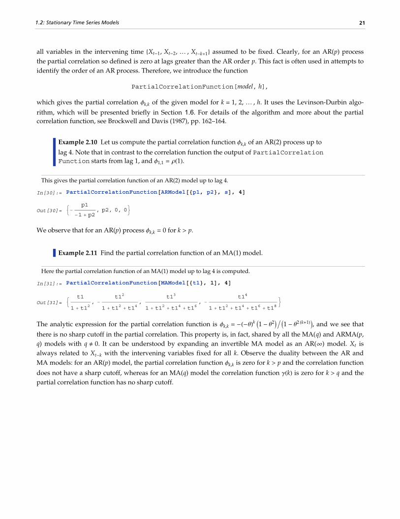
Example 2.10 Let us compute the partial correlation function fk,k of an AR(2) process up to
lag 4. Note that in contrast to the correlation function the output of PartialCorrelationFunction starts from lag 1, and f1,1 = rH1L.
This gives the partial correlation function of an AR(2) model up to lag 4.
In[30]:= PartialCorrelationFunction@ARModel@8p1, p2<, sD, 4DOut[30]= :− p1
−1 + p2, p2, 0, 0>
We observe that for an AR(p) process fk,k = 0 for k > p.
Example 2.11 Find the partial correlation function of an MA(1) model.
Here the partial correlation function of an MA(1) model up to lag 4 is computed.
In[31]:= PartialCorrelationFunction@MAModel@8t1<, 1D, 4DOut[31]= : t1
1 + t12, −
t12
1 + t12 + t14,
t13
1 + t12 + t14 + t16, −
t14
1 + t12 + t14 + t16 + t18>
The analytic expression for the partial correlation function is fk,k = -H-qLk I1 - q2M ë I1 - q2 Hk+1LM, and we see that
there is no sharp cutoff in the partial correlation. This property is, in fact, shared by all the MA(q) and ARMA(p,q) models with q ∫ 0. It can be understood by expanding an invertible MA model as an AR(¶) model. Xt isalways related to Xt-k with the intervening variables fixed for all k. Observe the duality between the AR andMA models: for an AR(p) model, the partial correlation function fk,k is zero for k > p and the correlation function
does not have a sharp cutoff, whereas for an MA(q) model the correlation function gHkL is zero for k > q and thepartial correlation function has no sharp cutoff.
1.2: Stationary Time Series Models 21

Here is the plot of the partial correlation function of the MA(1) model in Example 2.11 with q1 = 0.8. Since the partial correlation function starts from lag 1, in contrast to the correlation function we can use ListLinePlot directly.
In[32]:= ListLinePlot@PartialCorrelationFunction@[email protected]<, 1D, 20D,AxesLabel −> 8"k", "φk,k"<, PlotLabel −> "Partial correlation function"D
Out[32]=
5 10 15 20k
−0.3
−0.2
−0.1
0.1
0.2
φk,k
Partial correlation function
1.2.5 Multivariate ARMA Models
In some cases, at each time t, several related quantities are observed and, therefore, we want to study thesequantities simultaneously by grouping them together to form a vector. By so doing we have a vector or multivar-iate process. It is straightforward to generalize the definition of a univariate ARMA model to the multivariatecase. Let Xt = HXt 1, Xt 2, … , Xt mL£ and Zt = HZt 1, Zt 2, … , Zt mL£ be m-dimensional random vectors (here £ denotestranspose). A zero-mean, m-variate ARMA(p, q) model is defined by
(2.11) Xt - F1 Xt-1 - … - Fp Xt-p = Zt + Q1 Zt-1 + … + Qq Zt-q
where the AR and MA coefficients 8Fi< (i = 1, 2, … , p) and 8Qi<, (i = 1, 2, … , q) are all real mäm matrices and thezero-mean white noise 8Zt< is characterized by a covariance matrix S. Again, it is useful to define the matrix ARpolynomial FHxL and the matrix MA polynomial QHxL by
FHxL = I - F1 x - F2 x2 - … - Fp xp
and
QHxL = I + Q1 x + Q2 x + … + Qq xq,
where I denotes the mä m identity matrix. Now (2.11) can be written as F HBL Xt = Q HBL Zt, where B is the back-ward shift operator.
22 Time Series

As in the univariate case, a multivariate ARMA(p, q) model is represented by the object
ARMAModel[8F1, F2,… , Fp<, 8Q1, Q2, … , Qq<, S]
where each parameter matrix must be entered according to Mathematica convention. For example, the AR(1)model
Xt 1
Xt 2=
f11 f12
f21 f22
Xt-11
Xt-12+
Zt 1
Zt 2
with noise covariance S (Si j = si j) is represented as
ARModel[888f11, f12<, 8f21, f22<<<, 88s11, s12<, 8s21, s22<<].
The various quantities defined in the univariate case can be extended to the multivariate case. We proceed to dothis and illustrate how they are computed.
Stationarity and Invertibility
The definitions of mean, variance, and covariance, and the stationarity condition can be extended straightfor-wardly to a multivariate process. Now the mean is a vector and the variance and covariance are matrices. Theyare defined as follows:
mean: m HtL = E Xt ,
variance: S HtL = Var HXtL = E HXt - m HtLL HXt - m HtLL£, and
covariance: G Hs, rL = Cov HXs, XrL = E HXs - m HsLL HXr - m HrLL£.
The stationarity condition for a multivariate ARMA model can be translated into the algebraic condition that allthe roots of the determinantal equation †FHxL§ = 0 lie outside the unit circle.
Example 2.12 As an exercise in using Mathematica, we illustrate how to explicitly check if the bivariate AR(1) model Xt - F1 Xt-1 = Zt is stationary where F1 = 880.6, -0.7<, 81.2, -0.5<<.
We first define the determinant. Here IdentityMatrix[2] generates the 2ä2 identity matrix.
In[33]:= eq = Det@IdentityMatrix@2D − 880.6, −0.7<, 81.2, −0.5<< xD;This solves the equation.
In[34]:= Solve@eq == 0, xDOut[34]= 88x → 0.0925926 − 1.35767 <, 8x → 0.0925926 + 1.35767 <<
1.2: Stationary Time Series Models 23

We now find the absolute values of the roots.
In[35]:= Abs@x ê. %DOut[35]= 81.36083, 1.36083<Since both roots lie outside the unit circle, we conclude that the model is stationary.
In fact, all the Mathematica functions introduced previously for the univariate case have been designed so thatthey can be used with appropriate input for multivariate time series as well. Specifically, here we use the func-tion StationaryQ directly to check the stationarity of the bivariate AR(1) model of Example 2.12.
The model is stationary.
In[36]:= StationaryQ@[email protected], −0.7<, 81.2, −0.5<<<, 881, 0<, 80, 1<<DDOut[36]= True
Similarly, a multivariate ARMA model is invertible if all the roots of †QHxL§ = 0 are outside the unit circle. Theinvertibility of a model can be checked using InvertibleQ as in the univariate case.
Example 2.13 Check if the bivariate MA(2) model is invertible where Q1 = 88-1.2, 0.5<, 8-0.3, 0.87<<, and Q2 = 880.2, 0.76<, 81.1, -0.8<<.
The model is not invertible.
In[37]:= InvertibleQ@MAModel@888−1.2, 0.5<, 8−0.3, 0.87<<, 880.2, 0.76<, 81.1, −0.8<<<, 881, 0<, 80, 1<<DDOut[37]= False
A stationary ARMA model can be expanded as an MA(¶) model Xt = ⁄j=0¶ Yj Zt-j with YHBL = F-1HBL QHBL; simi-
larly, an invertible ARMA model can be expressed as an AR(¶) model ⁄j=0¶ Pj Xt-j = Zt with PHBL = Q-1HBL FHBL.
Again, the function ToARModel[model, p] can be used to obtain the order p truncation of an AR(¶) expansion.Similarly ToMAModel[model, q] yields the order q truncation of an MA(¶) expansion. 8Yj< and 8Pj< are matrices
and they are determined by equating the coefficients of corresponding powers of B in FHBL YHBL = QHBL andFHBL = QHBL PHBL, respectively.
Example 2.14 Expand the following AR(1) model as an approximate MA(3) model.
This expands the given AR(1) as an MA(3) model.
In[38]:= ToMAModel@[email protected], 0<, 8−0.1, 0.8<<<, 881, 0<, 80, 1<<D, 3DOut[38]= [email protected], 0.<, 8−0.1, 0.8<<, 880.04, 0.<, 8−0.1, 0.64<<,880.008, 0.<, 8−0.084, 0.512<<<, 881, 0<, 80, 1<<D
24 Time Series

Covariance and Correlation Functions
The matrix covariance function of a stationary multivariate process is defined by
G HkL = E HXt+k - mL HXt - mL£.
Note that now GHkL ∫ G H-kL; instead we have GHkL = GH-kL£. It is easy to see that the ith diagonal element of GHkL,GHHkLLi i ª gi iHkL = E Xt+k,i Xt i, is simply the (auto)covariance of the univariate time series 8Xt i< and
GHHkLLi j ª gi jHkL = E Xt+k,i Xt j is the cross-covariance of the series 8Xt i< and 8Xt j<. The matrix correlation function
RHkL is defined by
RHHkLLi j = ri jHkL = gi jHkL í gi iH0L gj jH0L .
Note that unlike the univariate case, we cannot simply divide GHkL by GH0L to get the correlation function.
We can get the covariance or correlation function of a multivariate ARMA model up to lag h simply by usingCovarianceFunction[model, h] or CorrelationFunction[model, h]; the output consists of a list ofmatrices 8GH0L, GH1L, … GHhL< or 8RH0L, RH1L, … , RHhL<.
Example 2.15 Find the covariance function of a bivariate MA(1) model up to lag 3.
This gives the covariance function of a bivariate MA(1) model up to lag 3.
In[39]:= cov = CovarianceFunction@MAModel@888t1, t2<, 8t3, t4<<<, IdentityMatrix@2DD, 3DOut[39]= 9991 + t12 + t22, t1 t3 + t2 t4=, 9t1 t3 + t2 t4, 1 + t32 + t42==,88t1, t2<, 8t3, t4<<, 880, 0<, 80, 0<<, 880, 0<, 80, 0<<=These are covariance matrices 8GH0L, GH1L, GH2L, GH3L< and they can be put into a more readable form using TableForm .
The covariance function is displayed in a table form.
In[40]:= TableForm@Transpose@8Table@gamma@iD, 8i, 0, 3<D, cov<DDOut[40]//TableForm=
gamma@0D 1 + t12 + t22 t1 t3 + t2 t4t1 t3 + t2 t4 1 + t32 + t42
gamma@1D t1 t2t3 t4
gamma@2D 0 00 0
gamma@3D 0 00 0
Again, the covariance function vanishes for lags greater than q (=1 in this case).
1.2: Stationary Time Series Models 25

Often we want to get the cross-covariance or cross-correlation of two processes i and j by extracting the (i, j)element of each matrix in the output of CovarianceFunction or CorrelationFunction, respectively.Whenever we want to do the same operation on each entry of a list, we can use the Mathematica function Map.For example, to get the cross-covariance function of processes 1 and 2, g12HkL, for k ¥ 0 in the above bivariateMA(1) model, we can do the following.
We extract the cross-covariance function using Map.
In[41]:= cov@@All, 1, 2DDOut[41]= 8t1 t3 + t2 t4, t2, 0, 0<Similarly, we can get the autocovariance of process 2 of the bivariate MA model in Example 2.15 by extractingthe (2, 2) element of each covariance matrix.
We use Map again to extract the covariance function of process 2.
In[42]:= cov@@All, 2, 2DDOut[42]= 91 + t32 + t42, t4, 0, 0=
Example 2.16 Compute the cross-correlation of a bivariate ARMA(1, 1) process and plot it.
The correlation function of the given ARMA(1, 1) process is computed. Recall that the semicolon is used at the end of an expression to suppress the display of the output.
In[43]:= corr = CorrelationFunction@[email protected], −0.9<, 81.1, −0.7<<<,8880.4, −0.8<, 81.1, −0.3<<<, 881, 0.5<, 80.5, 1.2<<D, 20D;Notice that AR and MA parameter matrices are enclosed in separate lists and the noise variance is a symmetricpositive-definite matrix. First we extract the cross-correlation g12HkL and then plot it.
This extracts the cross-correlation function.
In[44]:= %@@All, 1, 2DDOut[44]= 80.573964, −0.792494, −0.27461, 0.562118, 0.0633266, −0.372421, 0.0339551, 0.231558,
−0.0680429, −0.134589, 0.0704652, 0.0720437, −0.0595065, −0.0342067, 0.0449255,0.0129072, −0.0313338, −0.00199385, 0.0204524, −0.00281441, −0.0125266<
26 Time Series

Here is the cross-correlation plot. The option PlotRange is set to All to prevent the truncation of any large values in the plot.
In[45]:= plotcorr@%, Joined −> True, PlotRange −> All, AxesLabel −> 8"k", "RHkL1,2"<D
Out[45]= 5 10 15 20k
−0.8
−0.6
−0.4
−0.2
0.2
0.4
0.6
RHkL1,2
In contrast to autocorrelation, the cross-correlation at lag 0 is, in general, not equal to 1. Note that we haveplotted the cross-correlation only for k ¥ 0. Here we demonstrate how to plot the cross-correlation function fromlags -h to h. First we must obtain 8g12H-hL, g12H-h + 1L, … , g12H0L, g12H1L, … , g12HhL<. This can be accomplishedusing the fact that g12H-kL = g21HkL.
This gives the cross-correlations from lag -20 to lag 20. Drop[list, n] gives list with its first n elements dropped and Drop[list, -n] gives list with its last n elements dropped.
In[46]:= gamma12 = Join@Reverse@corr@@All, 2, 1DDD, Drop@corr@@All, 1, 2DD, 1DD;Using gamma12 as an example, it is convenient to define a function, say, plotmulticorr, to plot multivariatecorrelations. The argument should include the multivariate correlation function and i and j indicating whichcross-correlation or autocorrelation is to be plotted.
This defines the function plotmulticorr.
In[47]:= plotmulticorr@corr_, i_, j_, opts___D :=ListPlot@Join@Reverse@corr@@All, j, iDDD, Drop@corr@@All, i, jDD, 1DD,DataRange −> H8−1, 1< HLength@corrD − 1LL, optsD
Now we can plot the cross-correlation function of the above example using plotmulticorr.
1.2: Stationary Time Series Models 27

This plots the same cross-correlation function but now from lag -20 to 20. Note that it is not symmetric about the origin.
In[48]:= plotmulticorr@corr, 1, 2, Joined −> True,
PlotRange −> All, AxesLabel −> 8"k", "RHkL1,2"<D
Out[48]=−20 −10 10 20
k
−0.8
−0.6
−0.4
−0.2
0.2
0.4
0.6
RHkL1,2
We can also plot the correlation of series 1 of the bivariate ARMA(1, 1) process of Example 2.16 for lags from-20 to 20 using plotmulticorr.
This plots the correlation function of series 1. In contrast to the plot of the cross-correlation function, the graph is, of course, symmetric.
In[49]:= plotmulticorr@corr, 1, 1, Joined −> True,
PlotRange −> All, AxesLabel −> 8"k", "RHkL1,1"<D
Out[49]=
−20 −10 10 20k
−0.5
0.5
1.0
RHkL1,1
28 Time Series
Partial Correlation Function
The direct extension of the partial correlation function to the multivariate case leads to what is often calledpartial autoregressive matrices. The partial autoregressive matrix at lag k is the solution Fk,k to the Yule-Walker
equations of order k. (See Section 1.6 for a description of Yule-Walker equations and the Levinson-Durbinalgorithm.) However, here we will refer to them as the partial correlation function and use PartialCorrelationFunction[model, h] to obtain these matrices up to lag h, but bear in mind that some authors definepartial correlation function for a multivariate process differently, for example, Granger and Newbold (1986), p.246.
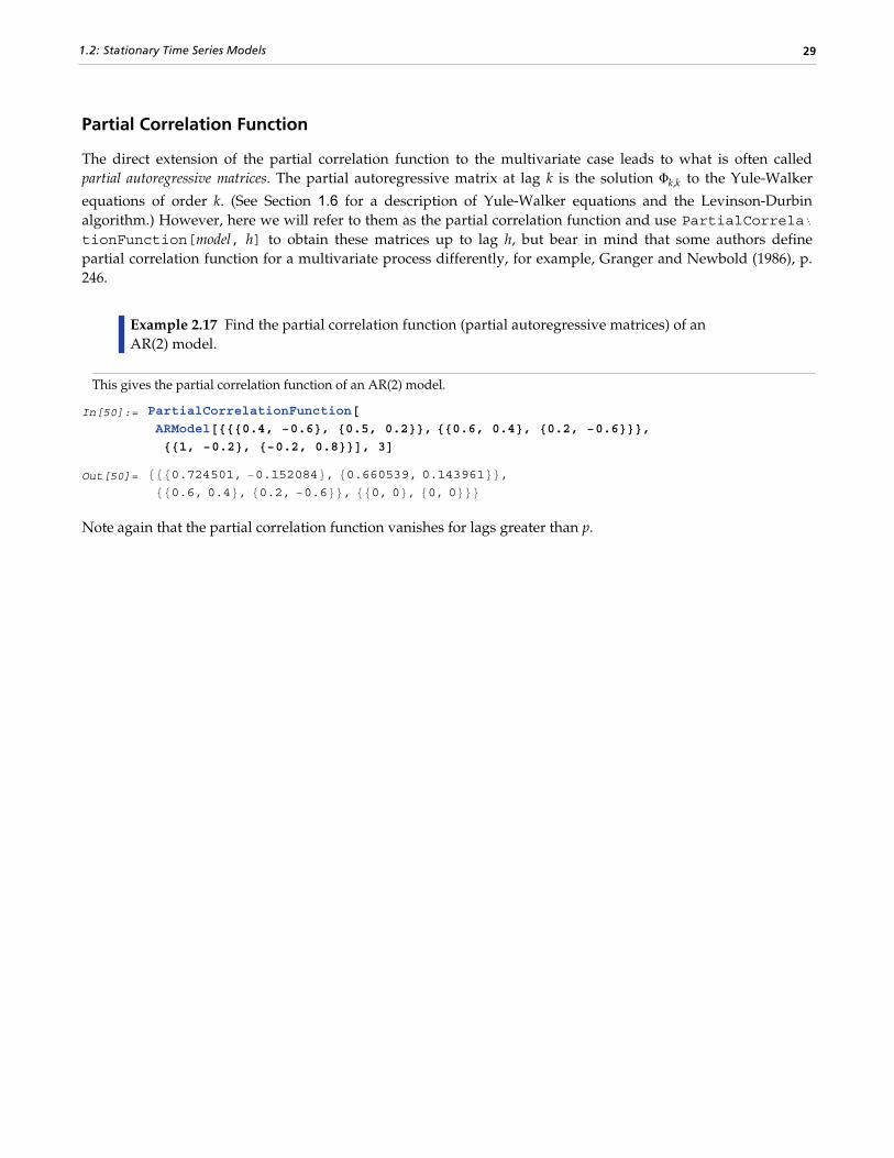
Example 2.17 Find the partial correlation function (partial autoregressive matrices) of an AR(2) model.
This gives the partial correlation function of an AR(2) model.
In[50]:= PartialCorrelationFunction@[email protected], −0.6<, 80.5, 0.2<<, 880.6, 0.4<, 80.2, −0.6<<<,881, −0.2<, 8−0.2, 0.8<<D, 3D
Out[50]= 8880.724501, −0.152084<, 80.660539, 0.143961<<,880.6, 0.4<, 80.2, −0.6<<, 880, 0<, 80, 0<<<Note again that the partial correlation function vanishes for lags greater than p.
1.2: Stationary Time Series Models 29

1.3 Nonstationary and Seasonal ModelsIn this section we first introduce a special class of nonstationary ARMA processes called the autoregressiveintegrated moving average (ARIMA) process. Then we define seasonal ARIMA (SARIMA) processes. After present-ing the objects that define these processes we proceed to illustrate how the various functions introduced inSection 1.2 in the context of ARMA models can be applied directly to ARIMA and SARIMA models. The func-tion that converts them to ARMA models is also introduced.
1.3.1 ARIMA Process
When the ARMA model fHBL Xt = qHBL Zt is not stationary, the equation fHxL = 0 (or †FHxL§ = 0 in the multivariatecase) will have at least one root inside or on the unit circle. In this case, the methods of analyzing stationary timeseries cannot be used directly. However, the stationary ARMA models introduced in Section 1.2 can be general-ized to incorporate a special class of nonstationary time series models. This class of models is characterized byall the zeros of the AR polynomial being outside the unit circle with the exception of d of them which are 1. Inother words, this class of nonstationary models is defined by
(3.1) H1 - BLd fHBL Xt = qHBL Zt,
where d is a non-negative integer, fHxL and qHxL are polynomials of degrees p and q, respectively, and all theroots of fHxL = 0 are outside the unit circle. Equation (3.1) defines an autoregressive integrated moving averageprocess of orders p, d, q, or simply, ARIMA(p, d, q).
Using the definition of the backward shift operator B, we have H1 - BL Xt = Xt - Xt-1. This operation is for obvi-ous reasons called differencing the time series. (We use H1 - BL2 Xt = H1 - BL HXt - Xt-1L = Xt - 2 Xt-1 + Xt-2 todifference the time series twice.) Equation (3.1) says that if 8Xt< is nonstationary and satisfies (3.1), then afterdifferencing the time series d times the differenced series 8Yt< (Yt = H1 - BLd Xt) is stationary and satisfiesfHBL Yt = qHBL Zt, that is, an ARMA(p, q) process. Note that we can view 8Yt< as a filtered version of 8Xt< (seeSection 1.4.3).
Therefore, any ARIMA(p, d, q) series can be transformed into an ARMA(p, q) series by differencing it d timesand, thus, the analysis of an ARIMA process does not pose any special difficulty as long as we know the num-ber of times to difference (i.e., d) the series. We will see in Section 1.4.3 how the differencing is done in practice.
An ARIMA(p, d, q) model is represented by the object
ARIMAModel[d, 8f1, f2, … , fp<, 8q1, q2, … , qq<, s2].
An ARIMA(p, 0, q) process is simply an ARMA(p, q) process.

1.3.2 Seasonal ARIMA Process
Sometimes there can be seasonal or cyclic components in a time series. By this we mean the recurrence of somerecognizable pattern after some regular interval that we call the seasonal period and denote by s. For example, inthe monthly data of international airline passengers there is clearly a recurring pattern with a seasonal period of12.
A pure seasonal model is characterized by nonzero correlations only at lags that are multiples of the seasonalperiod s. This means that the time series at time t, Xt, depends on Xt-s, Xt-2 s, Xt-3 s, … only. In general, we candefine a pure seasonal ARMA model of orders P and Q and of seasonal period s by
(3.2) Xt - F1 Xt-s - F2 Xt-2 s - … - FP Xt-P s = Zt + Q1 Zt-s + … + QQ Zt-Q s.
If we define the seasonal AR polynomial FHxsL as
FHxsL = 1 - F1 xs - F2 x2 s - … - FP xP s
and the seasonal MA polynomial QHxsL as
QHxsL = 1 + Q1 xs + Q2 x2 s + … + QQ xQ s,
(3.2) can be rendered more compactly using the backward shift operator B as
FHBsL Xt = QHBsL Zt.
(Note that although we use the same notation F and Q for seasonal model parameters as for multivariate ARMAmodel parameters, their meaning should be clear from the context.)
The pure seasonal models defined by (3.2) are often not very realistic since they are completely decoupled fromeach other. That is, (3.2) represents s identical but separate models for Xt, Xt+1, … , Xt+s-1. In reality, of course,few time series are purely seasonal and we need to take into account the interactions or correlations between thetime series values within each period. This can be done by combining the seasonal and regular effects into asingle model. A multiplicative seasonal ARMA model of seasonal period s and of seasonal orders P and Q andregular orders p and q is defined by
(3.3) fHBL FHBsL Xt = qHBL QHBsL Zt.
Here fHxL and qHxL are regular AR and MA polynomials defined in (2.4) and (2.5).
To generalize the model defined by (3.3) to include nonstationary cases we define the seasonal difference to beH1 - BsL Xt = Xt - Xt-s. A multiplicative seasonal autoregressive integrated moving average (SARIMA) process of periods, with regular and seasonal AR orders p and P, regular and seasonal MA orders q and Q, and regular andseasonal differences d and D is defined by
(3.4) H1 - BLd H1 - BsLD fHBL FHBsL Xt = qHBL QHBsL Zt.
We will use SARIMA(p, d, q)(P, D, Q)s to refer to the model defined by (3.4). In typical applications, D = 1 and Pand Q are small.
1.3: Nonstationary and Seasonal Models 31

A SARIMA(p, d, q)(P, D, Q)s model is represented by the object
SARIMAModel[8d, D<, s, 8f1, … , fp<, 8F1, … , Fp<, 8q1, … , qq<,8Q1, … , QQ<,s2].
Note that a pure seasonal model (3.2) and a seasonal ARMA model (3.3) are special cases of the SARIMAmodel, and we do not use different objects to represent them separately. If a particular order is zero, for exam-ple, p = 0, the parameter list 9f1, … , fp= is 8< or 80<. For example, ARMAModel[8<,8q<, 1] is the same asARMAModel[80<,8q<,1] and as MAModel[8q<, 1].
Any SARIMA process can be thought of as a particular case of a general ARMA process. This is because we canexpand the polynomials on both sides of (3.4) and obtain an ARMA(p + P s + d + s D, q + s Q) model whoseARMA coefficients satisfy certain relationships. Similarly, an ARIMA model defined in (3.1) is a special case ofthe ARMA(p + d, q) model. If we wish to expand a SARIMA or an ARIMA model as an equivalent ARMAmodel, we can invoke the function
ToARMAModel[model].
Example 3.1 Convert the ARIMA(1, 3, 2) model H1 - BL3 H1 - f1 BL Xt = I1 + q1 B + q2 B2M Zt to the equivalent ARMA(4, 2) model.
We load the package.
In[1]:= Needs@"TimeSeries`TimeSeries`"DThis converts the given ARIMA model to the equivalent ARMA model.
In[2]:= ToARMAModelAARIMAModelA3, 8φ1<, 8θ1, θ2<, σ2EEOut[2]= ARMAModelA83 + φ1, −3 − 3 φ1, 1 + 3 φ1, −φ1<, 8θ1, θ2<, σ2E
Example 3.2 Convert the SARIMA(1, 2, 1)(1, 0, 1)3 model H1 - BL2 H1 - f1 BL I1 - F1 B3M Xt = H1 + q1 BL I1 + Q1 B3M Zt to the equivalent ARMA model.
This converts the SARIMA model to the equivalent ARMA model.
In[3]:= ToARMAModelASARIMAModelA82, 0<, 3, 8φ1<, 8Φ1<, 8θ1<, 8Θ1<, σ2EEOut[3]= ARMAModelA82 + φ1, −1 − 2 φ1, φ1 + Φ1, −2 Φ1 − φ1 Φ1, Φ1 + 2 φ1 Φ1, −φ1 Φ1<, 8θ1, 0, Θ1, θ1 Θ1<, σ2EThis is an ARMA(6, 4) model. In contrast to an arbitrary ARMA(6, 4) model, this model has only four indepen-dent ARMA parameters.
The functions introduced earlier for ARMA models are applicable to ARIMA and SARIMA models as well.These functions convert the ARIMA and SARIMA models to ARMA models internally and then compute thedesired quantities. In the following we provide a few illustrative examples of the usage.
Example 3.3 Check if the SARIMA(0, 0, 1)(0, 1, 2)2 model
32 Time Series

I1 - B2M Xt = H1 - 0.5 BL I1 - 0.5 B2 + 0.9 B4M Zt is invertible.
This SARIMA model is invertible.
In[4]:= InvertibleQ@SARIMAModel@80, 1<, 2, 80<, 80<, 8−0.5<, 8−0.5, 0.9<, 1DDOut[4]= True
Example 3.4 Expand the above SARIMA model as an approximate AR(7) model.
This expands the SARIMA model as an AR(7) model.
In[5]:= ToARModel@SARIMAModel@80, 1<, 2, 80<, 80<, 8−0.5<, 8−0.5, 0.9<, 1D, 7DOut[5]= ARModel@8−0.5, 0.25, 0.125, 1.2125, 0.60625, 0.428125, 0.214063<, 1DSince the covariance or correlation function is defined only for stationary models, any attempt to calculate thecovariance or correlation function of a SARIMA or an ARIMA model with d ∫ 0 or D ∫ 0 will fail.
The model is nonstationary and no correlation is calculated.
In[6]:= CorrelationFunction@SARIMAModel@80, 1<, 12, 80<, 80.5<, 80.8<, 80<, 1D, 5DCovarianceFunction::nonst :The model SARIMAModel@80, 1<, 12, 80<, 80.5<, 80.8<, 80<, 1D is not stationary.
Out[6]= CorrelationFunction@SARIMAModel@80, 1<, 12, 80<, 80.5<, 80.8<, 80<, 1D, 5DExample 3.5 Find the covariance function of a pure seasonal model I1 - F1 B3M Xt = I1 + Q1 B3M Zt.
This is the covariance function of a pure seasonal model.
In[7]:= CovarianceFunctionASARIMAModelA80, 0<, 3, 8<, 8Φ1<, 8<, 8Θ1<, σ2E, 7EOut[7]= :− σ2 I1 + Θ12 + 2 Θ1 Φ1M
−1 + Φ12
, 0, 0,
−σ2 IΦ1 + Θ12 Φ1 + Θ1 I1 + Φ12MM
−1 + Φ12
, 0, 0, −σ2 Φ1 IΦ1 + Θ12 Φ1 + Θ1 I1 + Φ12MM
−1 + Φ12
, 0>As expected, the covariance function of a pure seasonal model is nonzero only at lags that are multiples of theseasonal period s. The values of the covariance function at lags 0, s, 2 s, … are the same as those of a regularARMA(P, Q) model with the same parameters. In fact, the two models are identical if we rescale time by a factors in the pure seasonal model. In our current example, the values of the covariance function at lags 0, 3, 6, … arethe same as those at lags 0, 1, 2, … of the regular ARMA(1, 1) model H1 - F1 BL Xt = H1 + Q1 BL Zt.
1.3: Nonstationary and Seasonal Models 33

This is the covariance function of the regular ARMA(1, 1) model. Compare it with the previous expression.
In[8]:= CovarianceFunctionAARMAModelA8Φ1<, 8Θ1<, σ2E, 2EOut[8]= :− σ2 I1 + Θ12 + 2 Θ1 Φ1M
−1 + Φ12
, −σ2 IΦ1 + Θ12 Φ1 + Θ1 I1 + Φ12MM
−1 + Φ12
, −σ2 Φ1 IΦ1 + Θ12 Φ1 + Θ1 I1 + Φ12MM
−1 + Φ12
>Since a SARIMA(p, 0, q)(P, 0, Q)s model is an ARMA(p + s P, q + s Q) model, all the properties of the correlationand partial correlation functions we discussed in Sections 1.2.3 and 1.2.4 remain true. For example, the partialcorrelation function, fk,k, of a SARIMA(p, 0, 0)(P, 0, 0)s model vanishes for k > p + s P, and the correlation func-
tion, rHkL, of a SARIMA(0, 0, q)(0, 0, Q)s model vanishes for k > q + s Q. However, in some special cases we cansay more about the correlation function of a seasonal ARMA model due to the relationships that exist between
the coefficients. For example, the Hq + s QLth degree polynomial qHBL QHBsL can be expanded as
qHBL QHBsL = qHBL + Q1 Bs qHBL + Q2 B2 s qHBL + … + QQ BQ s qHBL.It is clear from the above expression that if s > q + 1 there are "gaps" in the above polynomial, that is, terms fromBq+1 to Bs-1, from Bs+q+1 to B2 s-1, … are absent. Now consider a seasonal ARMA model with p = P = 0. Thecovariance function is given by
(3.5) gHkL = EHqHBL QHBsL Zt qHBL QHBsL Zt-kL.If these "gaps" are large enough, for some values of k the covariance function gHkL vanishes simply because thereis no overlap between the polynomials on the right-hand side of (3.5). In fact, if the "gap" Hs - 1L - Hq + 1L + 1 islarger than q or s ¥ 2 Hq + 1L, we have gHkL = 0 for q < k < s - q, s + q < k < 2 s - q, … , HQ - 1L s + q < k < Q s - q,and, of course, we always have gHkL = 0 for k > s Q + q.
It is also easy to show from (3.5) that as long as "gaps" exist (i.e., s > q + 1) in the expansion of the MA polynomi-als, the covariance function is symmetric about the lags that are multiples of the seasonal period. In otherwords, gHs - iL = gHs + iL, gH2 s - iL = gH2 s + iL, … for i = 1, 2, … , q.
Example 3.6 Find the correlation function of the SARIMA(0, 0, 1)(0, 0, 2)6 model with q1 = 0.9, Q1 = 0.6, and Q2 = 0.5.
Since p = P = 0 and s = 6 ¥ 2 Hq + 1L = 4, we expect the correlation function has the properties described above.
This calculates the correlation function up to lag 20 from the SARIMA model.
In[9]:= corr = CorrelationFunction@SARIMAModel@80, 0<, 6, 8<, 8<, 80.9<, 80.6, 0.5<, 1D, 20DOut[9]= 81., 0.497238, 0., 0., 0., 0.277959, 0.559006, 0.277959, 0.,
0., 0., 0.154422, 0.310559, 0.154422, 0., 0., 0., 0., 0., 0., 0.<We observe that (a) rHkL = 0 for k > s Q + q = 13; (b) rHkL = 0 for q = 1 < k < 5 = s - q ands + q = 7 < k < 11 = 2 s - q; and (c) gH5L = gH7L, gH11L = gH13L. We plot this correlation function.
34 Time Series

Here is the plot of the correlation function.
In[10]:= ListPlot@corr, Filling −> Axis, PlotRange −> All, AxesLabel −> 8"k", "ρHkL"<D
Out[10]=
The symmetry of the correlation gHkL about the lags that are multiples of the seasonal period s leads directly tothe conclusion that at lags k s (k integer) the correlations are in general symmetric local extrema. This is seenclearly in the above graph.
The properties derived above for the correlation function of seasonal ARMA models with p = P = 0 will nothold for general seasonal ARMA models. However, for some low-order seasonal models, which are often whatwe encounter in practice, the correlations at lags that are multiples of the seasonal period tend to be localextrema as shown in the following example. It is helpful to keep this in mind when identifying a seasonal modelalthough fluctuations often wash out all but the very pronounced local extrema in practice. (See Section 1.5 onmodel identification.)
1.3: Nonstationary and Seasonal Models 35

Example 3.7 Find the correlation function of the SARIMA(1, 0, 0)(1, 0, 1)12 model with f1 = 0.6, F1 = -0.6, and Q1 = -0.8.
This is the plot of the correlation function.
In[11]:= ListPlot@CorrelationFunction@SARIMAModel@80, 0<, 12, 80.6<, 8−0.6<, 8<, 8−0.8<, 1D, 40D,Filling −> Axis, PlotRange −> All, AxesLabel −> 8"k", "ρHkL"<D
Out[11]=
The calculation of the partial correlation function of a SARIMA model proceeds as in the case of an ARMAmodel. Again for q = Q = 0, the partial correlation function fk,k = 0 for k > p + s P.
Example 3.8 Find the partial correlation function of a SARIMA model.
This is the plot of the partial correlation function of a SARIMA model.
In[12]:= ListLinePlot@PartialCorrelationFunction@SARIMAModel@80, 0<, 6, 8<, 80.5<, 80.5<, 8−1.2<, 1D,20D, AxesLabel −> 8"k", "φk,k"<D
Out[12]=
5 10 15 20k
−0.2
−0.1
0.1
0.2
0.3
0.4
φk,k
Multivariate ARIMA and SARIMA models are again defined by (3.1) and (3.4), respectively, with fHBL, FHBsL,qHBL, and QHBsL being matrix polynomials. All the functions illustrated above can be used for multivariate mod-els; however, we will not demonstrate them here.
36 Time Series

1.4 Preparing Data for ModelingIn Sections 1.2 and 1.3 we introduced some commonly used stochastic time series models. In this section weturn our attention to actual time series data. These data can be obtained from real experiments or observationsover time or generated from numerical simulations of specified time series models. We consider these data to beparticular realizations of stochastic processes. Although we call both the stochastic process and its realizationtime series, we distinguish between them by using lower-case letters to denote the actual data and the corre-sponding upper-case letters to denote the random variables.
Several ways of transforming the raw data into a form suitable for modeling are presented in this section. Thesetransformations include linear filtering, simple exponential smoothing, differencing, moving average, and theBox-Cox transformation. We demonstrate how to generate normally distributed random sequences and timeseries from specified models and also show how to read in data from a file and plot them.
1.4.1 Plotting the Data
The first thing to do in analyzing time series data is to plot them since visual inspection of the graph can pro-vide the first clues to the nature of the series: we can "spot" trends, seasonality, and nonstationary effects. Oftenthe data are stored in a file and we need to read in the data from the file and put them in the appropriate formatfor plotting using Mathematica. We provide several examples below.
Example 4.1 As an illustrative example of how to read in data from a file, let us suppose that we have a file called file1.dat in the directory TimeSeries/Data. (Note that specification of files and directories depends on the system being used.) The file consists of two columns of numbers. The numbers in the first column are the times when the observations were made and those in the second column are the outcomes of observations, that is, the time series. We can look at the contents of file1.dat using FilePrint.
We load the package first.
In[1]:= Needs@"TimeSeries`TimeSeries`"D

This displays the contents of the file file1.dat in the directory TimeSeries/Data.
In[2]:= FilePrint@ToFileName@8"TimeSeries", "Data"<, "file1.dat"DD0.5 0.0911. 0.5951.5 0.5722. 0.2912.5 0.8653. 0.6233.5 0.4124. 0.9344.5 0.6575. 0.723
We use the ReadList command to read in these numbers and put them in a list.
We read in the time series data from the file file1.dat. The specification 8Number, Number< in ReadList makes each entry in the list a list of two numbers 8t, xt<.
In[3]:= data1 = ReadList@ToFileName@8"TimeSeries", "Data"<, "file1.dat"D, 8Number, Number<DOut[3]= 880.5, 0.091<, 81., 0.595<, 81.5, 0.572<, 82., 0.291<, 82.5, 0.865<,83., 0.623<, 83.5, 0.412<, 84., 0.934<, 84.5, 0.657<, 85., 0.723<<Now data1 defined above is in the right format for ListLinePlot.
We plot the data using ListLinePlot.
In[4]:= ListLinePlot@data1, AxesLabel −> 8"t", "xt"<D
Out[4]=
1 2 3 4 5t
0.2
0.4
0.6
0.8
xt
We can check if the data were in fact taken at equally spaced intervals by doing the following. First extract thetime coordinates.
The time coordinates are the first element of each data point.
In[5]:= tcoord = data1@@All, 1DDOut[5]= 80.5, 1., 1.5, 2., 2.5, 3., 3.5, 4., 4.5, 5.<
38 Time Series

Now take the differences of adjacent time coordinates and see if they give the same number.
The differences are the same.
In[6]:= Union@Drop@tcoord, 1D − Drop@tcoord, −1DDOut[6]= 80.5<So we see that in this case the data were indeed taken at constant time intervals. Since we have assumed allalong that the data are taken at equally spaced time intervals, it is often convenient to drop the time coordinateand consider just the time series. All time series data to be input to time series functions should be in the form8x1, x2, … , xn< where xi is a number for a scalar time series and a list, xi = 8xi 1, xi 2, … , xi m<, for an m-variate timeseries.
We can cast the above data in the form appropriate for input to time series functions by taking the second (i.e.,the last) entry from each data point.
This extracts the time series.
In[7]:= data = data1@@All, 2DDOut[7]= 80.091, 0.595, 0.572, 0.291, 0.865, 0.623, 0.412, 0.934, 0.657, 0.723<Now the data are in the right form to be used in time series functions.
If we plot the above data using ListLinePlot we will get the same plot as before except (a) the origin of timewill have been shifted and (b) it will be in different time units with the first entry in data corresponding to time1, and the second to time 2, and so on.
Here is the time plot for the same series.
In[8]:= ListLinePlot@data, AxesLabel −> 8"t", "xt"<D
Out[8]=
2 4 6 8 10t
0.2
0.4
0.6
0.8
xt
Example 4.2 Often the time series data are stored in a file without the time coordinates, as in the case of the lynx data in the file lynx.dat in the directory TimeSeries/Data. The file contains a series of numbers separated by blanks.
1.4: Preparing Data for Modeling 39

This reads in the contents of the file lynx.dat in the directory TimeSeries/Data.
In[9]:= lynxdata = ReadList@ToFileName@8"TimeSeries", "Data"<, "lynx.dat"D, NumberD;It is convenient to use the Mathematica function Short to find out if the data are in the appropriate formatwithout printing out all the numbers.
This gives the short form of lynxdata.
In[10]:= Short@lynxdata, 4DOut[10]//Short=8269, 321, 585, 871, 1475, 2821, 3928, 5943, 4950, 2577,
523, 98, 184, 279, 409, 2285, 2685, 80 , 81, 80, 108, 229, 399,1132, 2432, 3574, 2935, 1537, 529, 485, 662, 1000, 1590, 2657, 3396<
We can plot lynxdata directly using ListLinePlot as we have demonstrated in the previous plot. On theother hand, if we want the time plot to show the real times at which the data were taken, we can reverse theabove procedure of transforming data1 to data. Suppose the data were taken from time t1 to tn in intervals ofD t, Range[t1, tn, deltat] will generate a list of all the times at which data were taken. If D t is omitted thedefault value of 1 is assumed. In our lynx example, the data were taken annually from the year 1821 to the year1934.
This combines the time series with the time coordinates.
In[11]:= data1 = Transpose@8Range@1821, 1934D, lynxdata<D;We use Short to display data1.
In[12]:= Short@data1, 4DOut[12]//Short=881821, 269<, 81822, 321<, 81823, 585<, 81824, 871<, 81825, 1475<, 81826, 2821<, 102 ,81929, 485<, 81930, 662<, 81931, 1000<, 81932, 1590<, 81933, 2657<, 81934, 3396<<
Now if we plot data1 using ListLinePlot the horizontal axis corresponds to the "real" time.
40 Time Series

Here is the time plot of the lynx data.
In[13]:= ListLinePlot@data1, AxesLabel −> 8"year", "trappings"<D
Out[13]=
1840 1860 1880 1900 1920year
1000
2000
3000
4000
5000
6000
7000
trappings
Example 4.3 The file file2.dat has a set of bivariate data with column 1 containing series 1 and column 2 containing series 2, separated by commas. Again we employ ReadList to read the data.
We read in the data from file2.dat.
In[14]:= data1 = ReadList@ToFileName@8"TimeSeries", "Data"<, "file2.dat"D,Number, RecordSeparators −> 8","<D;
We have used the option RecordSeparators -> "," because of the presence of commas between the num-bers. To convert data1, which is now a long list of numbers, into the correct time series data format we putevery pair of numbers into a list using Partition.
We use Partition to put the data in the right form for a multivariate series.
In[15]:= data = Partition@data1, 2D;Here are a few elements of data.
In[16]:= Take@data, 5DOut[16]= 880.830546, 1.66549<, 8−0.353715, 3.68722<,8−0.63938, 6.08595<, 8−2.31622, 8.87918<, 8−4.08102, 8.14158<<We see that data is a bivariate time series of length 100. Again it is in the correct format of the form8x1, x2, … , xn< with the ith entry xi being a list of length 2.
To extract the ith time series from multivariate data we can use data[[All,i]]. Here are the plots of the twoseries of the bivariate series data.
1.4: Preparing Data for Modeling 41

This is the time plot of series 1 of the bivariate series in file2.dat.
In[17]:= ListLinePlot@data@@All, 1DD, AxesLabel −> 8"t", "x1 t"<D
Out[17]=20 40 60 80 100
t
−10
−5
5
x1 t
This is the time plot of series 2 of the bivariate series in file2.dat.
In[18]:= ListLinePlot@data@@All, 2DD, AxesLabel −> 8"t", "x2 t"<D
Out[18]=
20 40 60 80 100t
−10
−5
5
10
15
x2 t
1.4.2 Generating Time Series
Sometimes we may need to generate a time series 8x1, x2, … , xn< from a given process in order to explore ittheoretically or gain intuition about it. The simplest time series is a sequence of independently and identicallydistributed (IID) random numbers. We can use the function
RandomSequence[m,s2, n]
to generate a sequence of n random numbers distributed according to the normal distribution with mean m andvariance s2.
Example 4.4 Generate a random sequence of length 6 distributed according to the normal distribution with mean m = 0 and variance s2 = 1 (i.e., NH0, 1L).
42 Time Series

This generates a random sequence of length 6.
In[19]:= RandomSequence@0, 1, 6DOut[19]= 8−1.85264, −1.81359, −0.922332, 0.963026, 1.80357, −0.06322<It is usually a good idea to seed the random number generator using SeedRandom[seed] before generating anyrandom numbers so the calculation can be repeated if necessary.
Example 4.5 Generate a tri-variate random sequence of length 5 distributed normally with mean m = 80, 1, 0.5< and the covariance matrix S = 881, 0.5, 0<, 80.5, 1.2, 0.8<, 80, 0.8, 1.5<<.
The random number generator is seeded first.
In[20]:= SeedRandom@294587DThis generates the random sequence.
In[21]:= RandomSequence@80, 1, 0.5<, 881, 0.5, 0<, 80.5, 1.2, 0.8<, 80, 0.8, 1.5<<, 5DOut[21]= 880.811364, 3.09889, 1.91463<,8−0.838268, 2.18402, 2.44013<, 80.0939811, −0.127805, −1.28733<,80.0562101, 1.40061, 2.57561<, 8−0.534473, −0.45115, −0.812483<<Note that we have used SeedRandom so the above series can be reproduced if so desired. We reiterate that thecovariance matrix must be a symmetric, positive definite matrix. Otherwise no random numbers will be gener-ated.
No random numbers are generated when the covariance matrix is not symmetric or positive definite.
In[22]:= RandomSequence@80, 0<, 880.5, 0.2<, 80.3, 1<<, 5DRandomSequence::symm : Covariance matrix 880.5, 0.2<, 80.3, 1<< is not symmetric.
Out[22]= RandomSequence@80, 0<, 880.5, 0.2<, 80.3, 1<<, 5DInternally, RandomSequence uses RandomReal to generate a univariate random sequence of length n. Thecurrent default random number generator is used. Sequences generated prior to Version 6.0 of Mathematica canbe obtained by using the legacy generator via SeedRandom[Method->"Legacy"] or SeedRandom[seed,Method->"Legacy"].
We can similarly generate univariate random sequences according to the distributions of our choice. Pleaseconsult the Mathematica documentation for distributions included with Mathematica.
To generate a time series of length n, 8x1, x2, … , xn<, according to one of the models defined in earlier sections,we can use the function
TimeSeries[model, n].
It generates the series by iterating
xt = f1 xt-1 + … + fp xt-p + zt + q1 zt-1 + … + qq zt-q.
1.4: Preparing Data for Modeling 43

The noise 8zt< is generated from the normal distribution with zero mean and variance or covariance specified inmodel. For models with p ∫ 0, p random numbers from the same distribution as the noise are used as the initialvalues 8x-p+1, x-p+2, … , x0<. We can also generate time series with specified initial values of the series using
TimeSeries[model, n, 8x-p+1, x-p+2, ..., x0<]
and with a specified noise sequence 8z-q+1, z-q+2, … , zn< using
TimeSeries[model, 8z-q+1, z-q+2, ..., zn<, 8x-p+1, x-p+2, ..., x0<].
Note that both the p initial values and the noise sequence are enclosed in lists. For an m-variate series each xi orzi is a list of m numbers.
Like RandomSequence, TimeSeries uses the current default random number generator. Series generatedprior to Version 6.0 of Mathematica can be obtained by using the legacy generator via SeedRandom[Method->"Legacy"] or SeedRandom[seed, Method->"Legacy"].
Example 4.6 Generate a time series of length 10 according to the ARIMA(2, 1, 1) model H1 - BL I1 - 0.5 B + 0.8 B2M Xt = H1 - 0.5 BL Zt where the noise variance is 1.2.
The random number generator is seeded first.
In[23]:= SeedRandom@93846DThis generates the time series of length 10 from the given ARIMA(2, 1, 1) model.
In[24]:= TimeSeries@ARIMAModel@1, 80.5, −0.8<, 8−0.5<, 1.2D, 10DOut[24]= 87.42594, 9.02073, 5.46151, 0.68873,
3.07068, 7.17666, 6.36394, 3.06564, 3.01135, 5.1414<We can also generate a time series with a specified noise sequence.
Here we generate a random sequence of length 9 distributed uniformly on the interval [-1, 1].
In[25]:= HSeedRandom@2847D;RandomReal@8−1, 1<, 9DL
Out[25]= 80.5414, −0.272838, −0.673503, 0.306298,0.383461, −0.765174, 0.457336, −0.0909457, −0.59793<
This generates a time series with the noise sequence generated above. Note that here the noise variance can be omitted in the argument of the model object.
In[26]:= TimeSeries@[email protected], −0.5<, 80.7<D, %, 80.5, −0.3<DOut[26]= 8−0.203858, −0.755261, −0.214277, 0.932645, −0.203083, −0.585225, 0.213686, −0.326243<
Example 4.7 Generate a bivariate AR(1) series of length 6 with F1 = 880.3, -0.4<, 80.2, 1.2<<, noise covariance S = 880.5, 0.2<, 80.2, 1<<, and initial value x0 = 80.5, -0.1<.
44 Time Series

The random number generator is seeded first.
In[27]:= SeedRandom@3857DWe generate the required bivariate AR(1) time series of length 6. Note that the initial value x0 is enclosed in a list.
In[28]:= TimeSeries@[email protected], −0.4<, 80.2, 1.2<<<, 880.5, 0.2<, 80.2, 1<<D, 6, 880.5, −0.1<<D
Out[28]= 880.546434, −0.217747<, 8−0.161597, 0.188712<, 80.248326, −0.319944<,80.0985543, 0.0741225<, 80.718557, 1.49708<, 80.171007, 2.33348<<1.4.3 Transformation of Data
In order to fit a time series model to data, we often need to first transform the data to render them "well-behaved". By this we mean that the transformed data can be modeled by a zero-mean, stationary ARMA type ofprocess. We can usually decide if a particular time series is stationary by looking at its time plot. Intuitively, atime series "looks" stationary if the time plot of the series appears "similar" at different points along the timeaxis. Any nonconstant mean or variability should be removed before modeling. In this section we introduce avariety of methods of transforming the data.
Example 4.8 The time plot of the data contained in the file file3.dat is shown below.
This reads in the data.
In[29]:= data = ReadList@ToFileName@8"TimeSeries", "Data"<, "file3.dat"D, NumberD;Here is the time plot of data.
In[30]:= plot1 = ListLinePlot@data, AxesLabel −> 8"t", "xt"<D
Out[30]=
10 20 30 40 50t
10
20
30
xt
It is clear from the time plot that the series is not stationary since the graph shows a tendency to increase with t,signaling a possible nonconstant mean mHtL. A nonconstant mean mHtL is often referred to as a trend. A trend of atime series can be thought of as an underlying deterministic component that changes relatively slowly withtime; the time series itself can be viewed as fluctuations superimposed on top of this deterministic trend. Estimat-
1.4: Preparing Data for Modeling 45

ing the trend by removing the fluctuations is often called smoothing, whereas eliminating the trend in order toobtain a series with a constant mean is often called detrending.
There are various ways of estimating a trend. For example, we can assume that the trend can be approximatedby a smooth function and use a simple curve-fitting method. The Mathematica function Fit can be used to fit alinear combination of functions to the data using linear least squares method. In this example, we fit a quadraticfunction of t (i.e., a linear combination of 81, t, t2<) to the above data. Fitting a polynomial in t to time series datausing the least squares method is often referred to as polynomial regression.
This fits the data to a quadratic polynomial.
In[31]:= trend = Fit@data, 81, t, t^2<, tDOut[31]= 4.458 − 0.931377 t + 0.0284097 t2
This is the estimate of the trend. We can remove the trend and get the "detrended" data or residuals by subtract-ing the trend from the data.
The trend is removed.
In[32]:= data − Table@trend, 8t, 1, Length@dataD<D;Here is the time plot of the "detrended" data. Compared to the previous plot no apparent systematic trend remains.
In[33]:= ListLinePlotA%, AxesLabel −> 9"t", "x̂t"=E
Out[33]=
10 20 30 40 50t
−4
−2
2
4
6
xˆt
This series now appears suitable for modeling as a stationary process.
In using the curve fitting method for estimating the trend described above we implicitly assumed that a globalfunction fits the entire data. This is not always desirable and often methods of modeling the trend locally arepreferable. For example, a simple moving average can be used to estimate the trend. Let yt be the smoothedvalue (i.e., estimated trend) at t. A simple moving average of order r is defined by
yt = ‚i=0
r-1
xt-i ê r for t = r, r + 1, … n .
46 Time Series

Thus each new data point is the average of r previous data points. Short time fluctuations are averaged outleaving smoothed data, which we use as an estimate of the trend. The function
MovingAverage[data, r]
performs a simple moving average of order r on data and gives the smoothed data 8yt<. Instead of using identical weights in the above sum, we can generalize the simple moving average by allowingarbitrary weights 8c0, c1, … , cr<. This leads to a weighted moving average or linear filter. (An analysis of linearfilters in the frequency domain will be found in Section 1.8.2.) Application of a linear filter of weights8c0, c1, … , cr< to 8xt< produces the filtered series 8yt< given by
(4.1) yt = ‚i=0
r
ci xt-i for t = r + 1, r + 2, … , n .
This is sometimes referred to as a one-sided or causal filter and yt = ⁄i=-r£r ci xt-i as a two-sided filter. The filter
defined above is no less general than a two-sided one since a simple "time shifting" converts one kind of filter tothe other.
The function
MovingAverage[data, 8c0, c1, … , cr<]
applies a moving average with weights 8c0, c1, … , cr< to data. The weights are rescaled to sum to 1. For a moredetailed discussion of moving averages see Kendall and Ord (1990), pp. 28–34.
Another kind of moving average is the so-called exponentially weighted moving average or exponential smoothing. Inexponential smoothing, the weights decrease exponentially and the smoothed series is given by
yt = yt-1 + a Hxt - yt-1L, for t = 1, 2, … , n ;
where a is called the smoothing constant and is usually restricted to values between 0 and 1. An initial value of y0
is required to start the updating. The function
ExponentialMovingAverage[data, a]
performs exponential smoothing on data with smoothing constant a. The initial value is taken to be the firstelement in data. A different starting value y0 can be used by prepending y0 to data.
Example 4.9 Plot the time series generated from a random walk model.
An ARIMA(0, 1, 0) model is also called a random walk model. Here is the plot of 100 data points generated from arandom walk model.
The random number generator is seeded first.
In[34]:= SeedRandom@3845717D;
1.4: Preparing Data for Modeling 47

We generate the time series from the random walk model.
In[35]:= data = TimeSeries@ARIMAModel@1, 80<, 80<, 1D, 100D;This is the time plot of the series.
In[36]:= ListLinePlot@data, AxesLabel −> 8"t", "xt"<D
Out[36]=
20 40 60 80 100t
−14
−12
−10
−8
−6
−4
−2
xt
Again the graph shows that the data display a tendency to increase with t. We might infer that the process has anonconstant mean mHtL. However, we know that the ARIMA model defined in Section 1.3 has mean zero, so thisappearance of a nonstationary mean is the result of a single finite realization of a zero-mean nonstationaryprocess. This apparent trend is often termed a stochastic trend in contradistinction to the deterministic trend weintroduced earlier.
Differencing is an effective way of eliminating this type of trend and rendering the series stationary. Recall thatthe once-differenced data 8yt< is given by yt = xt - xt-1 = H1 - BL xt, and twice-differenced data byH1 - BL yt = xt - 2 xt-1 + xt-2 = H1 - BL2 xt. So the ARIMA(0, 1, 0) series after differencing is a stationary seriesH1 - BL xt = yt = zt. Similarly, an ARIMA(p, d, q) series can be transformed into a stationary series by differencing
the data d times. To difference the data d times and get H1 - BLd xt we can use
ListDifference[data, d].
Notice that differencing is really a particular kind of linear filtering and a polynomial trend of degree k can beeliminated by differencing the data k + 1 times.
Now we difference the above random walk data and plot the differenced series.
48 Time Series

The differenced data plotted here resembles a stationary series in contrast to the previous plot of the original data.
In[37]:= ListLinePlot@ListDifference@data, 1D, AxesLabel −> 8"t", "H1−BLxt"<D
Out[37]=
20 40 60 80 100t
−2
−1
1
2
H1−BLxt
So far we have dealt with eliminating a nonconstant mean present in the time series. Nonstationarity can also bedue to nonconstant variance. For example, in the plot of the airline data (Example 1.2) we see clearly an increasein the variance as t increases. Here we re-display its time plot for examination.
Example 4.10 Transform the airline data into a stationary series.
The contents of airline.dat are read and put into aldata.
In[38]:= aldata = ReadList@ToFileName@8"TimeSeries", "Data"<, "airline.dat"D, NumberD;The airline series is plotted here.
In[39]:= ListLinePlot@aldata, AxesLabel −> 8"t", "xt"<D
Out[39]=
20 40 60 80 100 120 140t
200
300
400
500
600
xt
1.4: Preparing Data for Modeling 49

We see that the variance, riding on the trend, is also changing with time. We need to transform the series into aconstant variance before modeling it further. To stabilize the variance, a nonlinear transformation such as alogarithmic or square-root transformation is often performed. In this example, we try a natural logarithmictransformation, yt = ln xt.
This is the time plot of the airline data after the logarithmic transformation. Note that Log[aldata] gives the logarithm of each of the entries of aldata.
In[40]:= ListLinePlot@Log@aldataD, AxesLabel −> 8"t", "lnHxtL"<D
Out[40]=
20 40 60 80 100 120 140t
5.5
6.0
lnHxtL
The variance now is stabilized. However, the trend is still present and there is the obvious seasonality of period12. The method of differencing can also be used to eliminate the seasonal effects. We define the seasonal differ-ence with period s as xt - xt-s = H1 - BsL xt.
We can difference the data d times with period 1 and D times with the seasonal period s and obtainH1 - BLd H1 - BsLD xt using
ListDifference[data, 8d, D<, s].
Here is the airline data after the logarithmic transformation and seasonal differencing with period 12.
The transformed data is further differenced.
In[41]:= data = ListDifference@Log@aldataD, 80, 1<, 12D;
50 Time Series

This is the plot of the differenced data.
In[42]:= ListLinePlotAdata, AxesLabel −> 9"t", "H1−B12LlnHxtL"=E
Out[42]=
20 40 60 80 100 120t
0.05
0.10
0.15
0.20
0.25
0.30
H1−B12LlnHxtL
We see that the periodic behavior or seasonal effect has been eliminated. The series after removal of the seasonalcomponent is often referred to as seasonally adjusted series or "deseasonalized" series. A further difference givesthe following plot.
The transformed data appear stationary.
In[43]:= ListLinePlotAListDifference@data, 1D, AxesLabel −> 9"t", "H1−BLH1−B12LlnHxtL"=E
Out[43]=
20 40 60 80 100 120t
−0.10
−0.05
0.05
0.10
H1−BLH1−B12LlnHxtL
This series H1 - BL I1 - B12M lnHxtL can be fitted to a stationary model.
In fact, the logarithmic transformation is a special case of a class of transformations called the Box-Cox transforma-tion. If we denote the transformed series by 8yt< and let l be a real constant, the Box-Cox transformation isdefined by
yt = Ixtl - 1M ë l for l ∫ 0
and
yt = ln xt for l = 0.
1.4: Preparing Data for Modeling 51

Different values of l yield different transformations. It is trivial to implement this transformation on Mathemat-ica. If data contains the time series data to be transformed then Idataλ − 1M ë λ
or
Log[data]
gives the transformed series.
Sometimes the nonstationarity can come from models not included in the ARIMA or SARIMA models. Forexample, the AR polynomial might have unit roots that are not 1. Since the AR coefficients are real, the complexroots on the unit circle will appear in complex conjugate pairs resulting in factors such asI1 - ei a BM I1 - e-i a BM = I1 - 2 cos a B + B2M in our AR polynomial. We can use ListCorrelate[81, -2 Cos[a],1<, data] to remove this kind of nonstationarity.
After the data have been rendered stationary, we are ready to fit an appropriate model to the data. This is thesubject of the next two sections.
52 Time Series

1.5 Estimation of Correlation Function andModel Identification
As stated in the beginning, given a set of time series data we would like to determine the underlying mecha-nism that generated the series. In other words, our goal is to identify a model that can "explain" the observedproperties of the series. If we assume that after appropriate transformations the series is governed by an ARMAtype of model, model identification amounts to selecting the orders of an ARMA model.
In general, selecting a model (model identification), estimating the parameters of the selected model (parameterestimation), and checking the validity of the estimated model (diagnostic checking) are closely related andinterdependent steps in modeling a time series. For example, some order selection criteria use the estimatednoise variance obtained in the step of parameter estimation, and to estimate model parameters we must firstknow the model. Other parameter estimation methods combine the order selection and parameter estimation.Often we may need to first choose a preliminary model, and then estimate the parameters and do some diagnos-tic checks to see if the selected model is in fact appropriate. If not, the model has to be modified and the wholeprocedure repeated. We may need to iterate a few times to obtain a satisfactory model. None of the criteria andprocedures are guaranteed to lead to the "correct" model for finite data sets. Experience and judgment formnecessary ingredients in the recipe for time series modeling.
In this section we concentrate on model identification. Since the correlation function is the most telling propertyof a time series, we first look at how to estimate it and then use the estimated correlation function to deduce thepossible models for the series. Other order selection methods will also be introduced. Parameter estimation anddiagnostic checking are discussed in Section 1.6.
1.5.1 Estimation of Covariance and Correlation Functions
We are given n observations 8x1, x2, … , xn< of a process 8Xt< and we would like to estimate the mean and thecovariance function of the process from the given data. Since, as we have mentioned before, the assumption ofstationarity is crucial in any kind of statistical inference from a single realization of a process, we will assume inthis section that the data have been rendered stationary using the transformations discussed in Section 1.4.
We use the sample mean X as the estimator of the mean of a stationary time series 8Xt<, (5.1) X = HX1 + X2 + … + XnL ê n
and the sample covariance function g` as the estimator of the covariance function of 8Xt<, (5.2) g
` HkL =
1
n ‚t=1
n-k IXt+k - XM IXt - XM.

That is, the expectation in (2.8) is replaced by an average over the series at different times. It should be borne inmind that X and g` defined in (5.1) and (5.2) are random variables, and for a particular realization of the timeseries 8x1, x2, … , xn< they give a particular estimate of the mean and the covariance function. Note that in thedefinition of the sample covariance, (5.2), the denominator is n although there can be fewer than n terms in thesum. There are other definitions of the sample covariance function that are slightly different from (5.2). Forexample, one definition uses n - k rather than n in the denominator. For the advantages of using (5.2), see thediscussions in Kendall and Ord (1990), Sections 6.2 and 6.3 and in Brockwell and Davis (1987), p. 213.
The sample correlation function r` is defined to be the normalized sample covariance function,
(5.3) r̀HkL = g̀HkL ë g̀ H0L.To calculate the sample mean from the given data we can use the function
Mean[data]
and to calculate the sample covariances and sample correlations up to lag k we can use the functions
CovarianceFunction[data, k] and CorrelationFunction[data, k].
Note that these are the same functions we used to calculate theoretical covariance and correlation functionsfrom a given model. The difference is in the first argument of these functions. To get the sample covariances orcorrelations from the given data, the first argument of these functions is the data instead of a model object.
In principle, we can calculate the covariance or correlation up to the maximum lag n - 1 where n is the length ofthe data. However, we should not expect g` HkL to be very reliable for k comparable to n since in this case there aretoo few terms contributing to the average in (5.2). However, if you want to calculate the correlation function upto the maximum lag often, you can define a function with the default lag value set to n - 1 as follows.
This loads the package.
In[1]:= Needs@"TimeSeries`TimeSeries`"DThe lag argument is omitted from the function mycorrelation and it is assumed to be n - 1.
In[2]:= mycorrelation@data1_, data2___D := CorrelationFunction@data1, data2, Length@data1D − 1DExample 5.1 Calculate the sample mean and sample correlation function from the data of length 500 generated from the AR(2) process Xt = 0.9 Xt-1 - 0.8 Xt-2 + Zt (see Example 2.6).
We first generate the series according to the AR(2) model ARModel[80.9, -0.8<, 1].
The random number generator is seeded first.
In[3]:= SeedRandom@48376D;This generates the time series of length 500 according to the given AR(2) model.
In[4]:= data = TimeSeries@[email protected], −0.8<, 1D, 500D;
54 Time Series

Here is the sample mean of the series.
In[5]:= Mean@dataDOut[5]= −0.0042064
As we would have expected, the sample mean is close to the true mean 0. Next we calculate the sample correla-tion r̀HkL up to lag k = 25 and plot it against k. The plot of r̀HkL versus the lag k is often referred to as the correlo-gram.
This calculates the sample correlation function of the series up to lag 25.
In[6]:= corr = CorrelationFunction@data, 25D;To plot the correlation function, we redefine the function plotcorr here.
In[7]:= plotcorr@corr_, opts___D :=
ListPlot@corr, DataRange −> 80, Length@corrD − 1<, PlotRange −> All, optsDHere is the plot of the sample correlation function. We call this plot g2 for future re-display.
In[8]:= g2 = plotcorr@corr, Joined −> True,
AxesLabel −> 8"k", "ρHkL"<, PlotStyle −> [email protected]<DD
Out[8]=
5 10 15 20 25k
−0.5
0.5
1.0
ρHkL
A dashed line is rendered due to the specification of the option PlotStyle. The number 0.02 inside Dashingspecifies the length of the line segments measured as a fraction of the width of the plot.
The theoretical correlation function calculated from the same model was displayed in Example 2.6. Here wedisplay it again for comparison.
1.5: Estimation of Correlation Function and Model Identification 55

This plots the theoretical correlation function of the AR(2) process.
In[9]:= g1 = plotcorr@CorrelationFunction@[email protected], −0.8<, 1D, 25D,AxesLabel −> 8"k", "ρHkL"<, Joined −> True, PlotLabel −> "Correlation Function"D
Out[9]=
5 10 15 20 25k
−0.5
0.5
1.0
ρHkL Correlation Function
We can see how well the sample correlation function of the AR(2) process actually approximates the true correla-tion function by juxtaposing the plots of both using the command Show.
The theoretical correlation function (solid line) and the sample correlation function (broken line) are displayed together here using Show.
In[10]:= Show@g1, g2D
Out[10]=
5 10 15 20 25k
−0.5
0.5
1.0
ρHkL Correlation Function
We see that the sample correlation r` HkL provides a reasonable approximation to the true correlation function
rHkL. Intuitively we also expect, by an application of the central limit theorem, that the larger the n, the better r`
approximates r. This is indeed the case as we shall see in the next section.
56 Time Series

1.5.2 The Asymptotic Distribution of the Sample Correlation Function
Let 8Xt< be a stationary process with the correlation function r. Let r HhL£ = HrH1L, rH2L, … , rHhLL andr`
HhL£ = Ir` H1L, r
` H2L, … , r` HhLM. It can be shown (see, for example, Brockwell and Davis (1987), p. 214) that under
certain general conditions r`
HhL has the asymptotic joint normal distribution with mean r HhL and variance C ê n asn Ø ¶. The Hi, jL element of the matrix C, ci j, is given by
(5.4) ci j = ‚
k=-¶
¶ ArHk + iL rHk + jL + rHk - iL rHk + jL + 2 rHiL rHjL r2HkL - 2 rHiL rHkL rHk + jL - 2 rHjL rHkL rHk + iLE.
This formula was first derived by Bartlett in 1946 and is called Bartlett's formula. Any stationary ARMA modelwith 8Zt< distributed identically and independently with zero mean and finite variance satisfies the conditionsof Bartlett's formula.
Hence for large n, the sample correlation at lag i, r` HiL, is approximately normally distributed with mean rHiL and
variance ci i ê n,
(5.5) Var Ir` HiLM = ci i ë n = ‚
k=-¶
¶ Ar2Hk + iL + rHk - iL rHk + iL + 2 r2HiL r2HkL - 4 rHiL rHkL rHk + iLE ë n.
Bartlett's formula, (5.4) or (5.5), is extremely useful since it gives us a handle on deciding whether a small valuein the sample correlation function is in fact significantly different from zero or is just a result of fluctuations dueto the smallness of n. Next we give two examples where Bartlett's formula is used to determine if the samplecorrelation is zero.
Example 5.2 For a sequence of identically and independently distributed white noise 8Zt<, rH0L = 1 and rHiL = 0 for i ∫ 0. The above formula, (5.5), reduces to (for i ∫ 0)
Var Ir` HiLM = 1 ë n.
That is, for large n, r` HiL is normally distributed with mean zero and variance 1 ê n for i = 1, 2, … , h. This implies
that 95 percent of the time the plot of r` should fall within the bounds ≤1.96 ë n . In practice, 2 rather than 1.96
is often used in calculating the bounds.
Here we generate a normally distributed random sequence of length 200 with mean 0 and variance 1.5. Thesample correlation function is calculated up to 50.
The random number generator is seeded first.
In[11]:= SeedRandom@586351D
1.5: Estimation of Correlation Function and Model Identification 57

This generates a random sequence of length 200 with distribution NH0, 1.5L.In[12]:= data = RandomSequence@0, 1.5, 200D;
The sample correlation function up to lag 50 is generated.
In[13]:= corr = CorrelationFunction@data, 50D;We can display this sample correlation function along with the bounds ≤2 ë 200 using Show.
The sample correlation function and the bounds are displayed here using Show. The function Plot is used to plot the two constant functions that form the bounds.
In[14]:= Show@plotcorr@corrD, Plot@8−2ê [email protected], 2 ê[email protected]<, 8x, 0, 50<,PlotStyle −> 88Black, [email protected]<D<<D, AxesLabel −> 8"k", "ρHkL"<D
Out[14]=
10 20 30 40 50k
0.2
0.4
0.6
0.8
1.0
ρHkL
We see that r` HkL falls within the bounds for all k > 0. We have no reason to reject the hypothesis that the set of
data constitutes a realization of a white noise process.
You can also define your own function that plots the given correlation function and the bounds. For example,you can define the following.
This defines the function that plots the correlation function and the bounds.
In[15]:= myplotcorr1@corr_, bound_, opts___D :=
Show@plotcorr@corr, Joined −> TrueD, Plot@8−bound, bound<,8x, 0, Length@corrD − 1<, PlotStyle −> 88Black, [email protected]<D<<D, optsDYou can also define a function that does the same plot as myplotcorr1 but uses the data rather than the correlation
function as an argument. Note that now the bound is fixed to be 2 ë n and the correlation is plotted to the maximum lag.
In[16]:= myplotcorr2@data_, opts___D := myplotcorr1@CorrelationFunction@data, Length@dataD − 1D, 2 êSqrt@Length@dataDD, optsD
58 Time Series
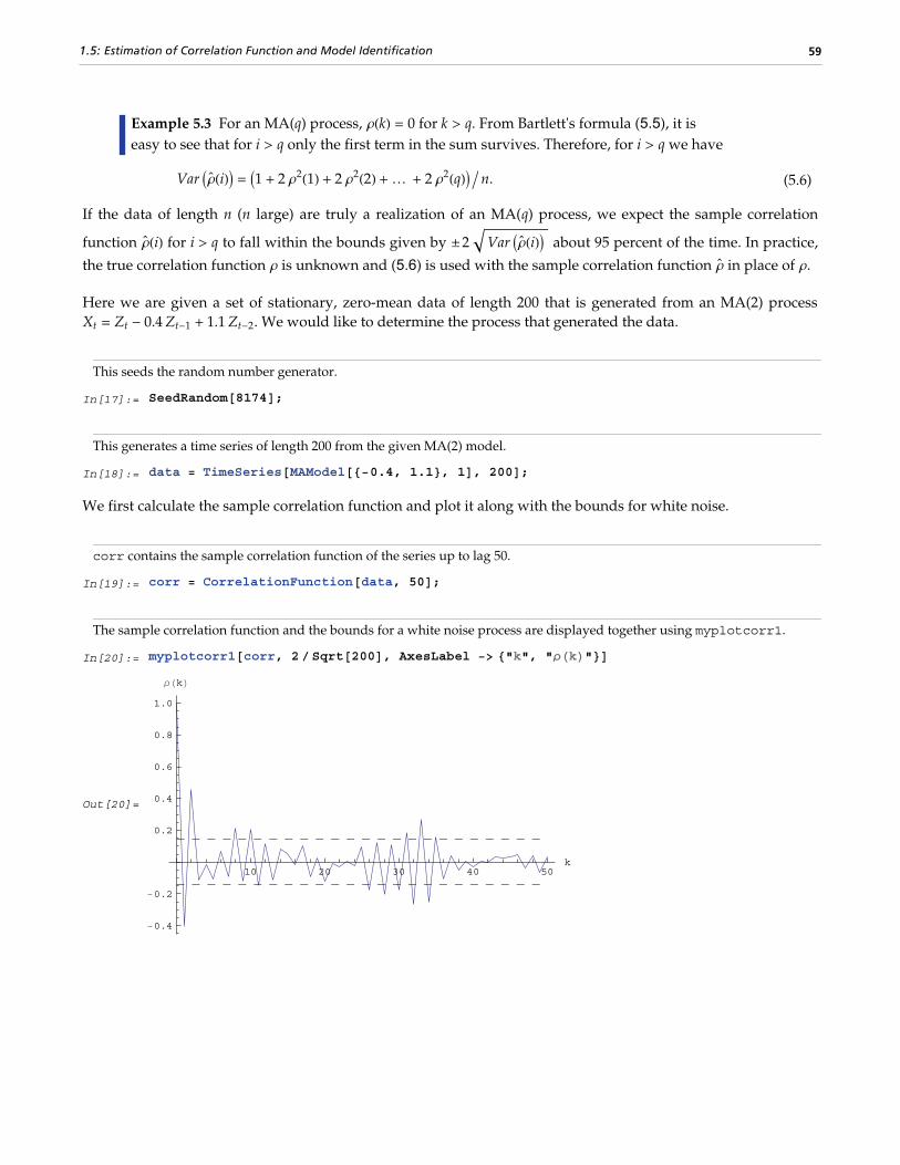
Example 5.3 For an MA(q) process, rHkL = 0 for k > q. From Bartlett's formula (5.5), it is easy to see that for i > q only the first term in the sum survives. Therefore, for i > q we have
(5.6) Var Ir` HiLM = I1 + 2 r2H1L + 2 r2H2L + … + 2 r2HqLM ë n.
If the data of length n (n large) are truly a realization of an MA(q) process, we expect the sample correlation
function r` HiL for i > q to fall within the bounds given by ≤2 Var Ir
` HiLM about 95 percent of the time. In practice,
the true correlation function r is unknown and (5.6) is used with the sample correlation function r` in place of r.
Here we are given a set of stationary, zero-mean data of length 200 that is generated from an MA(2) processXt = Zt - 0.4 Zt-1 + 1.1 Zt-2. We would like to determine the process that generated the data.
This seeds the random number generator.
In[17]:= SeedRandom@8174D;This generates a time series of length 200 from the given MA(2) model.
In[18]:= data = TimeSeries@MAModel@8−0.4, 1.1<, 1D, 200D;We first calculate the sample correlation function and plot it along with the bounds for white noise.
corr contains the sample correlation function of the series up to lag 50.
In[19]:= corr = CorrelationFunction@data, 50D;The sample correlation function and the bounds for a white noise process are displayed together using myplotcorr1.
In[20]:= myplotcorr1@corr, 2 ê Sqrt@200D, AxesLabel −> 8"k", "ρHkL"<D
Out[20]=
10 20 30 40 50k
−0.4
−0.2
0.2
0.4
0.6
0.8
1.0
ρHkL
1.5: Estimation of Correlation Function and Model Identification 59

Since the sample correlation function at lags 1 and 2, r` H1L and r
` H2L, are well beyond the bound, we conclude thatthey differ significantly from zero and the data are not likely to be random noise. Since the correlations beyondlag 2 are all rather small we may suspect that the data can be modeled by an MA(2) process. The variance of r
` HkLfor k > 2 can be calculated using (5.6), with the sample correlation function replacing the true correlation func-
tion, that is, we calculate J1 + 2 r` 2H1L + 2 r
` 2H2LN í n.
We first get the sample correlation up to k = 2. This is done by extracting the first three elements of corr usingTake.
This extracts the first three elements of corr.
In[21]:= Take@corr, 3DOut[21]= 81., −0.408219, 0.454923<
We square the list (each individual element will be squared) and then use Apply to add all the elements together.
In[22]:= H2 Total@%^2D − 1L ë 200Out[22]= 0.00873597
We have subtracted 1 to get rid of overcounting rH0L ( = 1). Now we can display the sample correlation functionagain with the bounds we just calculated.
The sample correlation function is displayed along with the newly calculated bounds.
In[23]:= myplotcorr1@corr, 2 Sqrt@%D, AxesLabel −> 8"k", "ρHkL"<D
Out[23]=
10 20 30 40 50k
−0.4
−0.2
0.2
0.4
0.6
0.8
1.0
ρHkL
This affirms the reasonableness of our conclusion that the data are from an MA(2) process.
60 Time Series
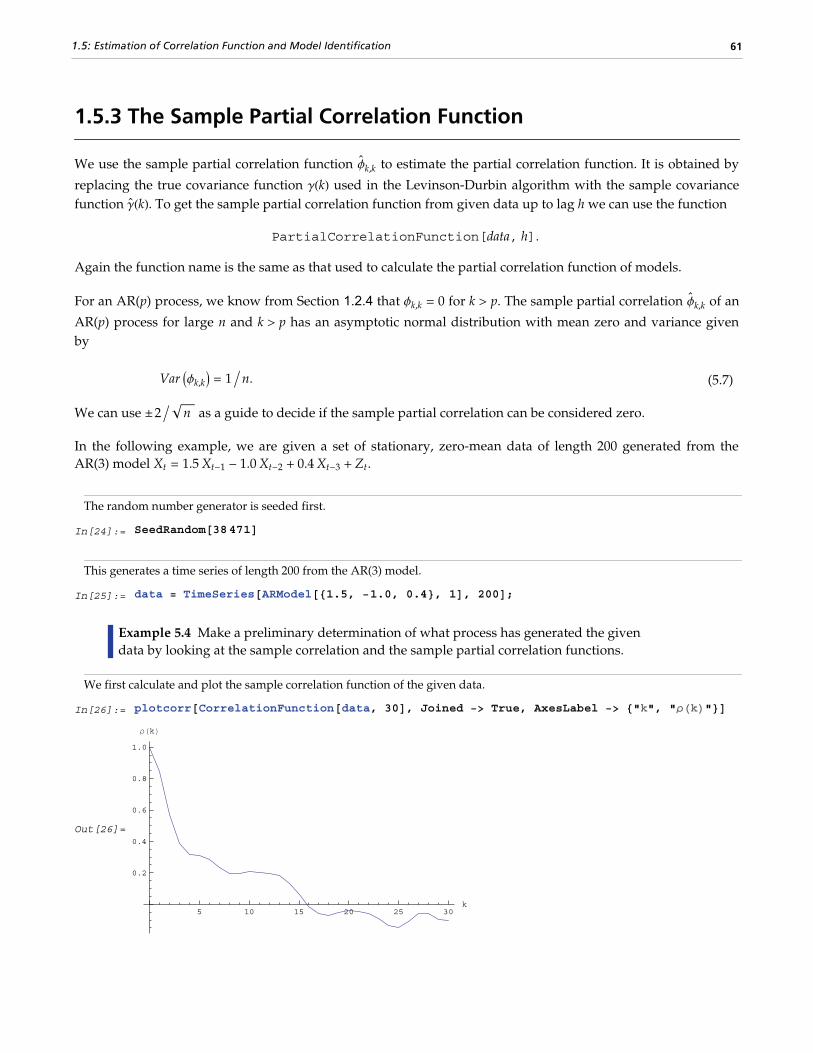
1.5.3 The Sample Partial Correlation Function
We use the sample partial correlation function f`
k,k to estimate the partial correlation function. It is obtained by
replacing the true covariance function gHkL used in the Levinson-Durbin algorithm with the sample covariancefunction g` HkL. To get the sample partial correlation function from given data up to lag h we can use the function
PartialCorrelationFunction[data, h].
Again the function name is the same as that used to calculate the partial correlation function of models.
For an AR(p) process, we know from Section 1.2.4 that fk,k = 0 for k > p. The sample partial correlation f`
k,k of an
AR(p) process for large n and k > p has an asymptotic normal distribution with mean zero and variance givenby
(5.7) Var Ifk,kM = 1 ë n.
We can use ≤2 ë n as a guide to decide if the sample partial correlation can be considered zero.
In the following example, we are given a set of stationary, zero-mean data of length 200 generated from theAR(3) model Xt = 1.5 Xt-1 - 1.0 Xt-2 + 0.4 Xt-3 + Zt.
The random number generator is seeded first.
In[24]:= SeedRandom@38471DThis generates a time series of length 200 from the AR(3) model.
In[25]:= data = TimeSeries@[email protected], −1.0, 0.4<, 1D, 200D;Example 5.4 Make a preliminary determination of what process has generated the given data by looking at the sample correlation and the sample partial correlation functions.
We first calculate and plot the sample correlation function of the given data.
In[26]:= plotcorr@CorrelationFunction@data, 30D, Joined −> True, AxesLabel −> 8"k", "ρHkL"<D
Out[26]=
5 10 15 20 25 30k
0.2
0.4
0.6
0.8
1.0
ρHkL
1.5: Estimation of Correlation Function and Model Identification 61

Since there is no sharp cutoff in the plot of the correlation function, it is unlikely that the data are from a pureMA process. Next we calculate and plot the sample partial correlation function. The plot of the sample partial
correlation function f`
k,k versus the lag k is sometimes referred to as the partial correlogram; we display the partial
correlogram of data together with the bounds ≤2 ë n .
The sample partial correlation function up to lag 30 is calculated from the given series data and defined to be pcf.
In[27]:= pcf = PartialCorrelationFunction@data, 30D;The sample partial correlation function is displayed along with the bounds using the function myplotcorr1 we defined in In[16].
In[28]:= myplotcorr1@pcf, 2 êSqrt@200D, AxesLabel −> 8"k", "φk,k"<D
Out[28]=
5 10 15 20 25k
−0.4
−0.2
0.2
0.4
0.6
0.8
φk,k
We see that the sample partial correlation differs from zero significantly only at the first 3 lags. This providesevidence to support the hypothesis that the data are from an AR(3) process.
1.5.4 Model Identification
There are various methods and criteria for selecting the orders of an ARMA model. We have seen in Sections1.5.2 and 1.5.3 that the correlogram and partial correlogram can provide powerful tools to determine the orderof a pure AR or MA process. So after the data have been transformed using the methods suggested in Section1.4, the first thing to do is to look at the correlogram and partial correlogram. The failure of the sample correla-tion function to decay to zero sufficiently fast signals that further differencing may be necessary to make thedata truly stationary.
Once the data are stationary, we can use our knowledge of theoretical correlation functions (see Section 1.2) ofdifferent models to deduce the possible ARMA orders for modeling our data. However, we must keep in mindthat sample correlation functions do not always resemble the true correlation functions as well as in Example5.1, especially in the small n case. Sample correlation at different lags can be highly correlated (see (5.4) for theexpression of covariance of r̀HiL and r̀HjL). Also it is easy to show that g̀ satisfies ⁄k=1
n-1 g̀ HkL = -1 ê 2, even though
the theoretical correlation function gHkL is strictly positive for all k. (That is, g` is biased.)
62 Time Series

Another type of order selection method is based on the so-called information criteria. The idea is to balance therisks of underfitting (selecting orders smaller than the true orders) and overfitting (selecting orders larger thanthe true orders). The order is chosen by minimizing a penalty function. The two commonly used functions are
(5.8) ln s` 2
+ 2 Hp + qL ê n
and
(5.9) ln s` 2
+ Hp + qL ln n ê n.
Here s` 2 is the estimated noise variance usually obtained from maximum likelihood estimations and n, as usual,is the length of the data. Akaike first suggested that the orders p and q be chosen such that they minimize thevalue of (5.8). This is called Akaike's information criterion (AIC). Similarly, using the minimum of (5.9) to selectorders is called using Bayesian information criterion (BIC). (Other definitions of AIC use the logarithm of thelikelihood function. See, for example, Brockwell and Davis (1987), p. 280.)
The first term in (5.8) and (5.9) can be interpreted as a penalty for underfitting, since the terms that are missingfrom the parameter fitting will be included in the noise and therefore give rise to an additional contribution tothe noise variance. The second term in (5.8) and (5.9) is directly proportional to the number of ARMA parame-ters and it is clearly the penalty for overfitting. Its effect is to favor a parsimonious model. Choosing a modelwith the smallest possible number of parameters is an important principle in model selection, and this principleis referred to as the principle of parsimony. See Box and Jenkins (1970), Section 1.3.
To get the AIC or BIC value of an estimated model we can simply use
AIC[model, n] or BIC[model, n].
Since the calculation of these values requires estimated noise variance, we will postpone demonstrating the useof these functions until Section 1.6.
A seasonal ARIMA(p, 0, q)(P, 0, Q)s model can, in principle, be treated as a special ARMA(p + s P, q + s Q) modelin model selection. However, since the number of independent parameters involved is often much smaller thanthat of a general ARMA(p + s P, q + s Q) model, the principle of parsimony dictates that we should determine s,P, and Q as well as p and q. This usually presents additional difficulties in order selection. However, if theorders of the seasonal models are small, which often seems to be the case in practice, we can determine theseasonal period s by inspecting the correlogram using the theoretical properties of the correlation function wediscussed in Section 1.3. The cutoff in the sample correlation or partial correlation function can suggest possiblevalues of q + s Q or p + s P. From this we can select the orders of regular and seasonal parts.
Example 5.5 A set of seasonal data of length 200 is given below. Determine the orders of the seasonal model that generated the data.
This seeds the random number generator.
In[29]:= SeedRandom@205967D;
1.5: Estimation of Correlation Function and Model Identification 63

This generates a time series of length 200 from the given SARIMA(1, 0, 0)(1, 0, 0)4 model.
In[30]:= data = TimeSeries@SARIMAModel@80, 0<, 4, 80.6<, 8−0.85<, 8<, 8<, 1D, 200D;First we look at the correlogram.
This gives the plot of the sample correlation function.
In[31]:= plotcorr@CorrelationFunction@data, 50D, Joined −> True, AxesLabel −> 8"k", "ρHkL"<D
Out[31]=
10 20 30 40 50k
−0.5
0.5
1.0
ρHkL
We see that the correlogram has extrema at lags that are multiples of 4. This suggests that s = 4. Since the correlo-gram has no sharp cutoff, the model is unlikely to be a pure MA model. Next we look at the sample partial
correlation function. We plot it along with the bounds ≤2 ë 200 .
The sample partial correlation function is displayed along with the bounds ≤2 ë 200 .
In[32]:= myplotcorr1@PartialCorrelationFunction@data, 30D,2 ê Sqrt@200D, AxesLabel −> 8"k", "φk,k"<D
Out[32]=5 10 15 20 25
k
−0.6
−0.4
−0.2
0.2
0.4
φk,k
64 Time Series
The partial correlogram has a cutoff at lag k = 5. We conclude that the model is a pure AR model withp + s P = 5. Given that s = 4, we may deduce that p = 1 and P = 1. This is, of course, an extremely simple exam-ple. In practice, model identification can be much more complicated.
For a mixed model we can select the orders using the AIC and BIC defined in (5.8) and (5.9) with p + q replacedby the number of seasonal model parameters p + P + q + Q.
1.5.5 Order Selection for Multivariate Series
For an m-variate series, Xt is a column vector of length m. The sample mean is again given by (5.1) andMean[data] gives the estimate of the mean vector. The definition of sample covariance in the multivariate caseis given by
G`
HkL =1
n ‚t=1
n-k IXt+k - XM IXt - XM£
and
G`
H-kL =1
n ‚t=k+1
n IXt-k - XM IXt - XM£
for 0 § k < n. The sample correlation function R` HHkLLi j = r
`i jHkL is defined to be
r`
i jHkL = g`
i jHkL í Ig` i iH0L g` j jH0LM1ê2,
where g` i jHkL = G` HHkLLi j. Note that the above equation reduces to (5.3), the univariate sample correlation, when
i = j.
In fact, the correlation function is the covariance function of the normalized or standardized series (i.e., a serieswith zero mean and unit variance), which is obtained by subtracting from each component its mean and divid-ing by its standard deviation.
Example 5.6 Calculate the sample correlation matrices up to lag 3 from the given bivariate data.
The random number generator is seeded first.
In[33]:= SeedRandom@479602DThis generates a bivariate time series of length 80 from the given MA(1) model.
In[34]:= data = TimeSeries@[email protected], −0.1<, 80.2, −0.8<<<, 881, 0<, 80, 1<<D, 80D;
1.5: Estimation of Correlation Function and Model Identification 65

The sample correlation function up to lag 3 is calculated and displayed in a table form.
In[35]:= TableForm@Transpose@8Table@rho@iD, 8i, 0, 3<D, CorrelationFunction@data, 3D<DDOut[35]//TableForm=
rho@0D 1. 0.175110.17511 1.
rho@1D 0.413944 −0.07186860.116806 −0.480424
rho@2D 0.128807 −0.02461430.0228069 0.0589108
rho@3D 0.13624 0.125488−0.0273056 −0.206116
We can get the same result by calculating the sample covariance function G of the standardized data. The datacan be standardized as follows.
The series generated from the given MA(1) model is standardized.
In[36]:= data1 = Transpose@HTranspose@dataD − Mean@dataDLê StandardDeviation@dataD
Sqrt@Length@dataDê HLength@dataD − 1LDD;Each component of the standardized series data1 has mean zero.
In[37]:= Mean@data1DOut[37]= 9−8.76035 ×10⁻¹⁷, −3.39626 × 10−18=
The covariance function of the standardized data up to lag 3 is calculated and tabulated.
In[38]:= TableForm@Transpose@8Table@gamma@iD, 8i, 0, 3<D, CovarianceFunction@data1, 3D<DDOut[38]//TableForm=
gamma@0D 1. 0.175110.17511 1.
gamma@1D 0.413944 −0.07186860.116806 −0.480424
gamma@2D 0.128807 −0.02461430.0228069 0.0589108
gamma@3D 0.13624 0.125488−0.0273056 −0.206116
This result is identical to the previous one. The variances of the series 1 and 2 are given by GHH0LL11 and GHH0LL22
and they are both 1. Also notice that GHkL º 0 for k > q = 1.
The methods of order selection employed in the univariate case can also be used for a multivariate series. Thefact that an AR(p) process has vanishing partial correlations at lags greater than p and an MA(q) process hasvanishing correlations at lags greater than q helps determine the order of an AR or MA process, respectively.For an MA(q) process, the asymptotic variance of the sample correlation r
`i jHkL (k > q) is given by
Var Ir̀i jHkLM =1
n 1 + 2 ‚
l=1
q
ri i HlL rj j HlL
66 Time Series

for all i and j. If the cross-correlation between two series ri jHkL vanishes for all k (i.e., the two series are uncorre-
lated) and one of the series is a white noise process, the above formula for the variance of r`
i jHkL reduces to
Var Ir̀i jHkLM = 1 ë n.
This result can be used to test if two series are independent of each other.
The sample partial correlation for a multivariate case is a direct extension of that for the univariate case. It iscalculated using the Levinson-Durbin algorithm. Again, PartialCorrelationFunction[data, h] gives thesample partial correlation function up to lag h.
The AIC and BIC of an m-variate process use the penalty functions
ln †S` § + 2 m2Hp + qL ë n
and
ln †S` § + 2 m2Hp + qL ln n ê n,
respectively. (†S` § denotes the determinant of S`.) They are again calculated using the functions AIC[model, n]
and BIC[model, n] and can be used to select the orders of an m-variate ARMA process.
1.5: Estimation of Correlation Function and Model Identification 67

1.6 Parameter Estimation and DiagnosticChecking
In this section different methods of estimating the ARMA parameters are presented: the Yule-Walker method,the Levinson-Durbin algorithm, Burg's algorithm, the innovations algorithm, the long AR method, the Hannan-Rissanen procedure, the maximum likelihood method, and the conditional maximum likelihood method.Functions calculating the logarithm of the likelihood function, the estimated information matrix, and the asymp-totic covariance of the maximum likelihood estimators are also given. Residuals and the portmanteau statisticused in the diagnostic checking can also be obtained with functions defined in this section.
1.6.1 Parameter Estimation
We first introduce some commonly used methods of estimating the parameters of the ARMA types of models.Each method has its own advantages and limitations. Apart from the theoretical properties of the estimators(e.g., consistency, efficiency, etc.), practical issues like the speed of computation and the size of the data mustalso be taken into account in choosing an appropriate method for a given problem. Often, we may want to useone method in conjunction with others to obtain the best result. These estimation methods, in general, requirethat the data be stationary and zero-mean. Failure to satisfy these requirements may result in nonsensicalresults or a breakdown of the numerical computation. In the following discussion we give brief descriptions ofeach estimation method in the time series package; for more details the reader is urged to consult a standardtime series text.
Yule-Walker Method
The Yule-Walker method can be used to estimate the parameters of an AR(p) model for a given p. If we multiplyeach side of (2.7) by Xt-k, k = 0, 1, … , p, and take expectations, we get a set of linear equations called the Yule-Walker equations:
(6.1) gHkL = f1 gHk - 1L + f2 gHk - 2L + … + fp gHk - pLfor k = 1, 2, … , p and
(6.2) gH0L - f1 gH1L - f2 gH2L - … - fp gHpL = s2.
The Yule-Walker equations can be solved for the covariance function g given the AR parameters (in fact, thefunction CovarianceFunction for AR models is obtained by solving the Yule-Walker equations) or they canbe solved for the AR coefficients 8fi< and the noise variance s2 if the covariance function is known. In practice,the exact covariance function is unknown and a natural way of getting an estimate of the AR parameters is touse the sample covariance function g` to replace the corresponding theoretical covariance function g in (6.1) and(6.2) and solve for 8fi< and s2. The solution so obtained is called the Yule-Walker estimate of the AR parame-

ters. In general, the method of estimating parameters by equating sample moments to theoretical moments isreferred to as the method of moments.
To estimate the parameters of an AR(p) model fitted to data using the Yule-Walker method we can use thefunction
YuleWalkerEstimate[data, p].
It gives the estimated model object
ARModel[8f`
1, f`
2, … , f`
p<,s` 2].
Example 6.1 Fit an AR(3) model to the data generated from the model Xt = 0.9 Xt-1 - 0.55 Xt-2 + 0.4 Xt-3 + Zt using the Yule-Walker method.
We load the package.
In[1]:= Needs@"TimeSeries`TimeSeries`"DThe random number generator is seeded first.
In[2]:= SeedRandom@304918D;A time series of length 120 is generated from the specified AR(3) model.
In[3]:= data = TimeSeries@[email protected], −0.55, 0.4<, 1D, 120D;Assuming that the order has been correctly identified we can proceed to estimate the parameters using the Yule-Walker method.
This gives the estimated AR(3) model using the Yule-Walker method.
In[4]:= YuleWalkerEstimate@data, 3DOut[4]= [email protected], −0.242644, 0.204865<, 0.829638DNote that the three numbers in the list are the estimated values of f1, f2, and f3, and the number 0.858176 is theestimated noise variance.
Levinson-Durbin Algorithm
Levinson and Durbin derived an iterative way of solving the Yule-Walker equations. Instead of solving (6.1)and (6.2) directly, which involves inversion of a päp matrix, the Levinson-Durbin algorithm fits AR models of
successively increasing orders AR(1), AR(2), … , AR(k) to the data. Let f`
m,j and s` m2 be the jth AR coefficient and
the noise variance of the fitted AR(m) model, respectively; the recursion formulas of the Levinson-Durbinalgorithm are (see Brockwell and Davis (1987), Section 8.2 and Morettin (1984))
1.6: Parameter Estimation and Diagnostic Checking 69

f`
m,m = g`
HmL - ‚j=1
m-1
f`
m-1,j g`
Hm - jL ì s`
m-12 ,
f`
m,k = f`
m-1,k - f`
m,m f`
m-1,m-k
for k = 1, 2, … , m - 1, and
s̀m2
= s̀m-12 J1 - f
`m,m2 N
with s` 02
= g` H0L.
The advantage of using the Levinson-Durbin algorithm over a direct solution of the Yule-Walker equations is
that it also gives us the partial correlations 8f`
1,1, f`
2,2, … <. (In fact, PartialCorrelationFunction uses the
Levinson-Durbin algorithm to compute the partial correlation function.) This allows us to select an appropriateAR model in the process of the parameter estimation. The function
LevinsonDurbinEstimate[data, k]
fits models AR(1), AR(2), … , AR(k) to data and gives a list of estimated model objects.
Example 6.2 Use the Levinson-Durbin algorithm to fit an AR model to the data used in Example 6.1.
This gives six estimated AR models of increasing order.
In[5]:= armodels = LevinsonDurbinEstimate@data, 6DOut[5]= [email protected]<, 0.873062D, [email protected], −0.0900402<, 0.865984D,
[email protected], −0.242644, 0.204865<, 0.829638D,[email protected], −0.209941, 0.101983, 0.134778<, 0.814568D,[email protected], −0.201451, 0.0845077, 0.196021, −0.0832399<, 0.808924D,[email protected], −0.205057, 0.0829532, 0.199726, −0.0969802, 0.0183952<, 0.80865D<
We can decide on the appropriate order by looking at the last AR(i) coefficient fi,i for i = 1, 2, … , 6. This is
precisely the sample partial correlation function defined earlier. To see this we can explicitly extract the lastnumber in the list of AR coefficients of each model.
The last AR coefficient of each model estimated above is extracted.
In[6]:= %@@All, 1, −1DDOut[6]= 80.683366, −0.0900402, 0.204865, 0.134778, −0.0832399, 0.0183952<Whenever we want to extract an element from the same position in each entry in a list, we can use the All partspecification. Here we wish to extract the last AR coefficient. The AR coefficients are the first parts of eachARModel and the last coefficient is the -1 part of that list.
70 Time Series

We get the same result using PartialCorrelationFunction.
In[7]:= PartialCorrelationFunction@data, 6DOut[7]= 80.683366, −0.0900402, 0.204865, 0.134778, −0.0832399, 0.0183952<We see that the partial correlations fall within the bound 2 ë 120 = 0.18 (see (5.7)) for k > 3. So we choose tomodel the data by an AR(3) process and the estimated model is the third entry in armodels.
This extracts the third entry in armodels.
In[8]:= armodels@@3DDOut[8]= [email protected], −0.242644, 0.204865<, 0.829638DNote that this is exactly the same as the result we got in Example 6.1 by using YuleWalkerEstimate.
We draw the attention of the reader to the behavior of the estimated noise variances. To see how they change asthe order of the model is varied, we extract and plot them.
The noise variances are extracted from armodels.
In[9]:= armodels@@All, −1DDOut[9]= 80.873062, 0.865984, 0.829638, 0.814568, 0.808924, 0.80865<
We plot the noise variance as a function of the AR model order p.
In[10]:= ListLinePlotA%, AxesLabel −> 9"p", "σ2"=, PlotRange −> AllE
Out[10]=
1 2 3 4 5 6p
0.82
0.83
0.84
0.85
0.86
0.87
σ2
We see that initially the variance drops as we increase the order of AR model to be fitted, and after p = 3 thevariance levels off. This gives an indication that the true order of the model is probably p = 3. This is because ifthe order of the fitted model is smaller than the true order, the noise variance will get an additional contributionfrom the terms that have been neglected and will be larger.
1.6: Parameter Estimation and Diagnostic Checking 71

Burg's Algorithm
Burg's algorithm (also referred to as the maximum entropy method) for estimating the AR parameters is alsoiterative, but it works directly with the data rather than with the sample covariance function. For large samples,Burg's algorithm is asymptotically equivalent to the Yule-Walker estimates although the two differ on smallsample properties. For a presentation of Burg's algorithm see Jones (1978). The function
BurgEstimate[data, k]
fits AR(1), AR(2), … , AR(k) models to data and gives a list of estimated model objects using Burg's algorithm.
Example 6.3 Use Burg's algorithm to fit an AR model to the data from the AR(3) model studied in Example 6.1.
This gives 5 estimated AR models using Burg's algorithm.
In[11]:= BurgEstimate@data, 5DOut[11]= [email protected]<, 0.872083D, [email protected], −0.0980994<, 0.863691D,
[email protected], −0.271324, 0.230368<, 0.817855D,[email protected], −0.236405, 0.130687, 0.128697<, 0.804309D,[email protected], −0.225461, 0.110888, 0.191081, −0.0837485<, 0.798668D<
This is the estimated AR(3) model. Compare it with the result of the Levinson-Durbin algorithm in Example 6.2.
In[12]:= %@@3DDOut[12]= [email protected], −0.271324, 0.230368<, 0.817855DInnovations Algorithm
For an MA model the method of moments involves solving a set of nonlinear equations and, therefore, it is notas convenient. Instead, other methods are used. The so-called innovations algorithm can be used to obtain apreliminary estimate of MA parameters.
Fitting MA(1), MA(2), … models to time series data using the innovations algorithm is analogous to fittingAR(1), AR(2), … models to data using the Levinson-Durbin algorithm. The iterative formulas and the details ofthe derivation can be found in Brockwell and Davis (1987), pp. 165–166 and Section 8.3.
The function
InnovationEstimate[data, k]
allows us to use the innovations algorithm to get an estimate of the MA parameters. It gives the estimatedmodels MA(1), MA(2), … , MA(k).
72 Time Series

Let q`
m,j be the jth MA coefficient of the estimated MA(m) model, then the asymptotic variance of q`
m,j can be
estimated to be
(6.3) s`
j2
= Var Hq`m,jL = 1 + ‚k=1
j-1
q`
m,k2 ì n,
and the order q is estimated to be the lag beyond which q`
m,j lies within ≤2 s`
j for j > q.
Once the order q is chosen, the estimated model parameters are given by q`
m,j for j = 1, 2, … , q where m is suffi-
ciently large that the values of q`
m,j have stabilized with respect to m. In contrast, in the Levinson-Durbin algo-
rithm, once the order of the AR process p is chosen, the estimated parameters for that p describe the estimatedmodel. To illustrate how to get the estimate of an MA model, we generate a set of data from an MA(2) processand then try to fit an MA model to it.
This seeds the random number generator.
In[13]:= SeedRandom@394587D;A time series of length 120 is generated from the given AR(2) model.
In[14]:= data = TimeSeries@MAModel@8−1.5, 0.7<, 1D, 120D;Example 6.4 Fit an appropriate ARMA model to the given stationary time series data.
We first look at the correlogram.
This calculates the sample correlation function up to lag 25.
In[15]:= corr = CorrelationFunction@data, 25D;To plot the correlation function, we redefine the function plotcorr here.
In[16]:= plotcorr@corr_, opts___D :=
ListPlot@corr, DataRange −> 80, Length@corrD − 1<, PlotRange −> All, optsD
1.6: Parameter Estimation and Diagnostic Checking 73

The above sample correlation function corr is plotted using the function plotcorr.
In[17]:= plotcorrAcorr, Joined −> True, AxesLabel −> 9"k", "ρˆHkL"=E
Out[17]=
5 10 15 20 25k
−0.5
0.5
1.0
ρˆHkL
We see that °r` HkL• is small H < 0.2L except for k § 2. We can conclude that the data are from an MA model ofrelatively small order. Next we calculate the bound for sample correlation function assuming q = 1 (see (5.6))
The bound for the sample correlation function is calculated under the assumption that q = 1.
In[18]:= 2 SqrtAH2 Total@Take@corr, 2D^2D − 1L ë 120EOut[18]= 0.253167
The value of r` H2L is within the bound.
In[19]:= corr@@3DDOut[19]= 0.170959
So MA(1) is a plausible model.
Now we use the innovations algorithm to determine the MA order and estimate the parameters.
74 Time Series

This gives ten estimated MA models of increasing order using the innovations algorithm.
In[20]:= mamodels = InnovationEstimate@data, 10DOut[20]= 8MAModel@8−0.679264<, 1.74834D, MAModel@8−1.04556, 0.170959<, 1.23994D,
MAModel@8−1.24477, 0.375973, 0.0464327<, 1.07071D,MAModel@8−1.3602, 0.478456, 0.000269039, −0.068144<, 0.966188D,MAModel@8−1.42063, 0.570985, 0.0215842, −0.0492007, 0.0613083<, 0.930046D,MAModel@8−1.42687, 0.647133, 0.0369225, −0.0341669, 0.0927607, −0.0167054<,0.929079D, MAModel@8−1.42865, 0.645337, −0.00497664, −0.0831326, 0.0378468,−0.0997403, −0.0544924<, 0.926231D, MAModel@8−1.43473, 0.644359, −0.0148594,−0.0982001, 0.0313664, −0.115448, −0.031991, 0.0548565<, 0.915075D,
MAModel@8−1.44321, 0.648848, −0.0134027, −0.0893809, 0.0510151,−0.098105, 0.0128691, 0.10665, 0.00380608<, 0.909607D,
MAModel@8−1.43844, 0.667823, −0.00788841, −0.0861545, 0.0709004,−0.070265, 0.0538966, 0.155801, 0.00864946, 0.00125505<, 0.906144D<
In order to compare the MA coefficients of the different models, let us extract and align them using the Mathemat-ica function Column.
The MA coefficients are extracted and aligned using Column.
In[21]:= NumberForm@Column@mamodels@@All, 1DDD, 2DOut[21]//NumberForm=8−0.68<8−1., 0.17<8−1.2, 0.38, 0.046<8−1.4, 0.48, 0.00027, −0.068<8−1.4, 0.57, 0.022, −0.049, 0.061<8−1.4, 0.65, 0.037, −0.034, 0.093, −0.017<8−1.4, 0.65, −0.005, −0.083, 0.038, −0.1, −0.054<8−1.4, 0.64, −0.015, −0.098, 0.031, −0.12, −0.032, 0.055<8−1.4, 0.65, −0.013, −0.089, 0.051, −0.098, 0.013, 0.11, 0.0038<8−1.4, 0.67, −0.0079, −0.086, 0.071, −0.07, 0.054, 0.16, 0.0086, 0.0013<
We see that the MA coefficients q`
m,j, j > 2, lie within the bound 2 ë 120 = 0.18 < 2 s̀j, suggesting that qj = 0 for
j > 2. (Although one number †q`9,8§ = 0.19 is larger than 0.18, it is within the bound 2 s`
2 given by (6.3).) Since the
MA coefficients q`
m,j, j § 2, are significantly different from zero, we conclude that q = 2.
The values of q`
m,1 and q`
m,2 stabilize around -1.5 and 0.78, respectively. In fact, for m ¥ 5 the fluctuations in qm,1
and qm,2 are of order 1 ë n . So any qm,1 and qm,2 for m ¥ 5 can be used as our estimated q1 and q2. We choosem = 7 and find the estimated parameters by selecting the first two coefficients of the MA(7) model. This can bedone conveniently using Mathematica.
This extracts the MA(7) model and keeps only the first two MA coefficients.
In[22]:= MapAt@Take@ , 2D &, mamodels@@7DD, 1DOut[22]= MAModel@8−1.42865, 0.645337<, 0.926231D
1.6: Parameter Estimation and Diagnostic Checking 75

Note that Map is used to perform an operation on all arguments while an operation on arguments only atspecified locations is accomplished using MapAt.
Long AR Method
For a mixed model ARMA(p, q), the above methods are not applicable and we must resort to other techniques.The long AR method can be used to estimate the parameters of ARMA(p, q) models as well as AR(p) and MA(q)models. We may recall that an invertible ARMA model can be approximated by an AR(k) model for sufficientlylarge values of k. The long AR method of estimating ARMA parameters makes use of this fact. It first fits anAR(k) model (k large, thus "long" AR method) to the data 8xt<,
xt = f1 xt-1 + … + fk xt-k + zt.
The estimated AR(k) coefficients 8f`
i< are obtained using the ordinary least squares regression method. Then
using the above equation with the 8f`
i< and data 8xt<, we can get the estimated residuals or innovations 8z`t<, z`t = xt - f
`1 xt-1 - … - f
`k xt-k.
Substituting these residuals into the ARMA(p, q) model we have,
xt = f1 xt-1 + f2 xt-2 + … + fp xt-p + q1 z̀t-1 + q2 z̀t-2 + … + qq z̀t-q + zt.
Now we can again use the ordinary least squares regression method to estimate the coefficients 8fi< and 8qi<, andthe noise variance is given by the residual sum of squares divided by the number of terms in the sum,
(6.4) ‚t=t£+1
n
zt2 ë Hn - t£L where t£ = max Hq + k, pL.
This procedure of fitting an invertible ARMA(p, q) model to data using the long AR method is encoded in thefunction
LongAREstimate[data, k, p, q],
where k is the order of long autoregression. Note that if the data are generated from a non-invertible model,long AR method fails and we may get nonsensical results.
Example 6.5 Fit an MA(2) model to the data in Example 6.4 using the long AR method.
The long AR method is used to obtain the estimated MA(2) model from data.
In[23]:= LongAREstimate@data, 8, 0, 2DOut[23]= MAModel@8−1.43634, 0.663807<, 0.994936D
Example 6.6 Estimate the parameters of an ARMA(1, 2) model from the data generated below.
76 Time Series

The random number generator is seeded first.
In[24]:= SeedRandom@31857D;A time series of length 150 is generated from the given ARMA(1, 2) model.
In[25]:= data = TimeSeries@[email protected]<, 80.2, −0.5<, 2D, 150D;This gives the estimated ARMA(1, 2) model using the long AR method. The order of the long autoregression is 10.
In[26]:= LongAREstimate@data, 10, 1, 2DOut[26]= [email protected]<, 80.0756134, −0.545209<, 1.4078DHannan-Rissanen Procedure
The idea behind the Hannan-Rissanen procedure of estimating ARMA parameters is very similar to that behindthe long AR method. That is, an AR(k) model is first fitted to the data in order to obtain the estimates of thenoise or innovation zt; when this estimated noise z̀t is used in place of the true noise it enables us to estimateARMA(p, q) parameters using the less expensive method of least squares regression. However, the basic differ-ence between the two methods is that in the long AR method the ARMA model orders to be fitted p and q aswell as the order of long autoregression k, are supplied, whereas in the Hannan-Rissanen method the orders aredetermined within the procedure itself using an information criterion. Specifically, the Hannan-Rissanen proce-dure consists of following steps.
1. Use the Levinson-Durbin algorithm to fit models AR(i), for i = 1, 2, … , kmax, to the data.
2. Calculate the AIC values ln s̀i2
+ 2 i ê n for i = 1, 2, … , kmax of the fitted AR models, and choose the model AR(k) that yields the smallest AIC value.
3. Calculate the residuals 8z̀t< from the fitted AR(k) model.
4. Estimate ARMA(p, q) coefficients using the least squares method for p § Min Hpmax, kL and q § qmax; the estimated noise variance is given again by (6.4).
5. Select the model that has the lowest BIC value (ln s`
p,q2
+ Hp + qL ln n ê n).
For more details on the Hannan-Rissanen procedure see Granger and Newbold (1986), pp. 82–83. The function
HannanRissanenEstimate[data, kmax, pmax, qmax]
selects an appropriate ARMA model to fit the data using the Hannan-Rissanen procedure.
Example 6.7 Use Hannan-Rissanen method to fit an ARMA model to the previous data.
The Hannan-Rissanen procedure selects as well as estimates the model. It chooses an MA(1) model for the same data.
In[27]:= HannanRissanenEstimate@data, 10, 3, 3DOut[27]= [email protected]<, 1.43075D
1.6: Parameter Estimation and Diagnostic Checking 77

Instead of getting the model with the lowest BIC value as selected by the Hannan-Rissanen procedure, some-times it is useful to know the models that have the next lowest BIC values. This can be done by specifying theoptional argument in HannanRissanenEstimate.
HannanRissanenEstimate[data, kmax, pmax, qmax, h]
gives h estimated models with increasing BIC values. Computationally this does not cost any extra time. It isadvisable to compare these h different models and decide on one in conjunction with other model identificationmethods. If you want to get all the models estimated in step 4 of the Hannan-Rissanen procedure, you can givea sufficiently large value of h. You can then select a model from these using your own criterion.
Here we use the procedure to print out four models with the lowest BIC values.
In[28]:= hrmodels = HannanRissanenEstimate@data, 10, 3, 3, 4DOut[28]= [email protected]<, 1.43075D, [email protected]<, 80.711995<, 1.42748D,
[email protected], 0.0241686<, 1.43976D,ARMAModel@8−0.122753, 0.142481<, 80.893641<, 1.41075D<
To find the BIC and AIC values of these models we can use Map.
We find the BIC values of each of the above four models. These values are in increasing order as they should be.
In[29]:= Map@BIC@ , 150D &, %DOut[29]= 80.391605, 0.422722, 0.431288, 0.444332<
The AIC values of the models can be found similarly.
In[30]:= Map@AIC@ , 150D &, %%DOut[30]= 80.371535, 0.38258, 0.391146, 0.384119<We see that while the MA(1) model has the lowest BIC value, the ARMA(1, 2) model has the lowest AIC value.Next we plot the sample correlation.
This calculates the sample correlation function up to lag 25.
In[31]:= corr = CorrelationFunction@data, 25D;
78 Time Series

The above sample correlation function is plotted here.
In[32]:= plotcorrAcorr, Joined −> True, AxesLabel −> 9"k", "ρˆHkL"=E
Out[32]=
5 10 15 20 25k
0.2
0.4
0.6
0.8
1.0
ρˆHkL
The bound for the sample correlation function is calculated under the assumption that q = 1.
In[33]:= 2 SqrtAH1 + 2 corr@@2DD^2L ë 150.EOut[33]= 0.19894
We see that although r̀H10L is beyond this bound, there is no strong evidence to reject the MA(1) model. Sobased on the above analysis either MA(1) or ARMA(1, 2) can be tentatively identified as the right model.
Maximum Likelihood Method
When the noise of a zero-mean, stationary ARMA process is normally distributed (8Zt< ~ NI0, s2M), we can getthe estimate of ARMA parameters by maximizing the Gaussian likelihood of the process. The parameters soobtained are called the maximum likelihood estimates of the parameters. The exact likelihood can be obtained fromthe prediction error decomposition (see Section 1.7) with the prediction errors being computed using the innova-tions algorithm. A complete discussion of the innovations algorithm and the calculation of the exact maximumlikelihood can be found in Brockwell and Davis (1987), Chapter 5 and Sections 8.3 and 8.4.
The function
LogLikelihood[data, model]
gives the logarithm of the exact Gaussian likelihood function for the given model and data. In the univariatecase, LogLikelihood gives what is called the "reduced likelihood" (see Brockwell and Davis (1987), p. 250)and in the multivariate case, it gives the logarithm of the full maximum likelihood (apart from a constant). SeeReinsel (1993), Section 5.4.
Example 6.8 Calculate the logarithm of the likelihood of the estimated ARMA(1, 2) model in Example 6.7.
1.6: Parameter Estimation and Diagnostic Checking 79

Here is the logarithm of the likelihood of the ARMA(1, 2) model estimated in Example 6.7.
In[34]:= LogLikelihood@data, hrmodels@@2DDDOut[34]= −0.372637
The maximum likelihood method of estimating model parameters is often favored because it has the advantageamong others that its estimators are more efficient (i.e., have smaller variance) and many large-sample proper-ties are known under rather general conditions.
MLEstimate[data, model, 8φ1, 8f11, f12<<, … ]
fits model to data using the maximum likelihood method. The parameters to be estimated are given in symbolicform as the arguments to model, and two initial numerical values for each parameter are required. Internally themaximization of the exact logarithm of the likelihood is done using the Mathematica built-in function FindMinimum and the same options apply. (To find out all the options of FindMinimum use Options[FindMinimum].)
Example 6.9 Use the maximum likelihood method to fit an MA(1) model and an ARMA(1, 2) model to the same data in Example 6.6.
The maximum likelihood estimate of the MA(1) model is obtained using MLEstimate.
In[35]:= model1 = MLEstimate@data, MAModel@8θ1<, 1D, 8θ1, 80.73, 0.74<<DOut[35]= [email protected]<, 1.40225D
Similarly, this is the maximum likelihood estimate of the ARMA(1, 2) model.
In[36]:= model2 = MLEstimate@data, ARMAModel@8φ1<, 8θ1, θ2<, 1D,8φ1, 80.1, 0.2<<, 8θ1, 80.6, 0.8<<, 8θ2, 80.1, 0.3<<DOut[36]= ARMAModel@8−0.583367<, 81.36826, 0.415562<, 1.38683D
This gives the logarithm of the likelihood of the latter model.
In[37]:= LogLikelihood@data, %DOut[37]= −0.336211
A couple of points of explanation are in order before we look at the results of our estimation. First, choosinggood starting values for the parameters to be estimated is very important in the maximum likelihood estimationsince not only can bad initial values slow down the calculation, but also abort the calculation if they reach theparameter region corresponding to nonstationary models. Since they are expected to be close to the values thatmaximize the likelihood, the estimated parameter values from other estimation methods are usually used asinitial values for the maximum likelihood estimation as we have done here. This is why some authors call allthe estimates of ARMA parameters that are not based on maximizing the likelihood function preliminaryestimates, and use them primarily as initial values in maximizing the likelihood. Second, the alert reader mayhave noticed that the noise variance is not entered as a symbolic parameter. This is because in the univariatecase, the likelihood function is independent of the noise variance and the noise variance is estimated separatelyat the end. So it does not matter what we input for the noise variance in the argument of the model, it is simplyignored. However, it is important that the noise variance should not be included in the parameter search list.
80 Time Series

This is because if extra parameters, which do not affect the value of the function being minimized, are includedin the search list, FindMinimum will fail to find a minimum.
Now we can select our model using AIC or BIC.
The MA(1) model is favored by AIC.
In[38]:= 8AIC@model1, 150D, AIC@model2, 150D<Out[38]= 80.35141, 0.367018<
The MA(1) model is also favored by BIC.
In[39]:= 8BIC@model1, 150D, BIC@model2, 150D<Out[39]= 80.371481, 0.427231<Both AIC and BIC favor the MA(1) model over the ARMA(1, 2) model. This result may be surprising, after all,we know that the data were generated from an ARMA(1, 2) model. However, when n is small it is possible thatother models can be fitted better to the data. More importantly, if the AR and MA polynomials fHxL and qHxL ofan ARMA model have an approximate common factor of degree g, an ARMA(p - g, q - g) model rather than anARMA(p, q) model is likely to be identified using information criteria.
In our example, the MA polynomial qHxL = 1 + 0.2 x - 0.5 x2 can be factorized asqHxL = H1 - 0.614143 xL H1 + 0.814143 xL.
The MA polynomial qHxL = 1 + 0.2 x - 0.5 x2 contains a factor close to H1 - 0.6 xL.In[40]:= Expand@H1 − 0.614143 xL H1 + 0.814143 xLDOut[40]= 1 + 0.2 x − 0.5 x2
We see that fHxL = H1 - 0.6 xL and qHxL share an approximate factor. This is why the data behave like an MA(1)model with q1 º 0.81.
The large discrepancy between the estimated ARMA(1, 2) parameters and the "true" model parameters f1 = 0.6,q1 = 0.2, and q2 = -0.5 can also be explained by this accidental presence of an approximate common factor.Consider a series of data 8xt< from an ARMA(p, q) model, fHBL xt = qHBL zt. It also satisfies an ARMA(p + g, q + g)model cHBL fHBL xt = cHBL qHBL zt, where cHBL is a polynomial of degree g. If we fit an ARMA(p + g, q + g) model tothe data, there is no unique solution and the maximum likelihood method can show strong dependence on theinitial conditions.
For example, if we change the initial conditions, we get quite different estimates from those in Out[36].
In[41]:= MLEstimate@data, ARMAModel@8φ1<, 8θ1, θ2<, 1D,8φ1, 80.1, 0.2<<, 8θ1, 80.7, 0.75<<, 8θ2, 8−0.1, −0.2<<DOut[41]= ARMAModel@8−0.583366<, 81.36826, 0.415561<, 1.38683D
1.6: Parameter Estimation and Diagnostic Checking 81

Conditional Maximum Likelihood Method
It is well known that the exact maximum likelihood estimate can be very time consuming especially when p + qis large. (We warn the user here that the function MLEstimate can be rather slow for large n or large number ofparameters.) Therefore, often, when the data length n is reasonably large, an approximate likelihood function isused in order to speed up the calculation. The approximation is made by setting the initial q values of the noisezp, zp-1, … , zp-q+1 to E Zt = 0 and fixing the first p values of X. The likelihood function so obtained is called theconditional likelihood function (conditional on zp = zp-1 = … = zp-q+1 = 0 and on X1, X2, … , Xp being fixed atx1, x2, … , xp). Maximizing the conditional likelihood function is equivalent to minimizing the conditional sumof squares function. So the conditional maximum likelihood estimate is the same as the conditional nonlinearleast squares estimate, and it is used as an approximation to the exact maximum likelihood estimate. Unlike thecase of the least squares estimate, the conditional maximum likelihood estimate of the noise variance is given bythe minimum value of the sum of squares divided by the effective number of observations n - p. The details ofthe conditional likelihood estimate are explained in Harvey (1981), Sections 5.2 and 5.3. See also Wilson (1973).
The function
ConditionalMLEstimate[data, model]
can be used to fit model to data using the conditional maximum likelihood estimate. It numerically searches forthe maximum of the conditional logarithm of the likelihood function using the Levenberg-Marquardt algorithmwith initial values of the parameters to be estimated given as the arguments of model.
Example 6.10 Fit a model to the data in Example 6.6 using the conditional maximum likelihood method.
We use the result from the Hannan-Rissanen estimate as our initial values. We can input the output of theearlier calculation directly.
The first model in hrmodels is used as the initial model to get the conditional maximum likelihood estimate of an MA(1) model.
In[42]:= ConditionalMLEstimate@data, hrmodels@@1DDDOut[42]= [email protected]<, 1.40202D
The second model in hrmodels is used as the initial model to get the conditional maximum likelihood estimate of the ARMA(1, 2) model.
In[43]:= arma12 = ConditionalMLEstimate@data, hrmodels@@2DDDOut[43]= ARMAModel@8−0.0895185<, 80.885883<, 1.40502DFor a pure AR model, the conditional maximum likelihood estimate reduces to a linear ordinary least squaresestimate and no initial parameter values are necessary. We can if we like simply use
ConditionalMLEstimate[data, p]
to fit an AR(p) model to data.
82 Time Series

The Asymptotic Properties of the Maximum Likelihood Estimators
Often we would like to know the approximate standard errors associated with our parameter estimates. Theseerrors can be obtained from the asymptotic covariance of the estimators. Let b = If1, f2, … , fp, q1, q2, … , qqM£
be
the parameters of a stationary and invertible ARMA(p, q) model and b`
the maximum likelihood or conditionalmaximum likelihood estimator of b. Then, it can be shown that as n Ø ¶,
n1ê2 Ib`
- bM fl N H0, V HbLL.To calculate V for a univariate ARMA model we can use the function
AsymptoticCovariance[model].
The function uses the algorithm given in Godolphin and Unwin (1983).
This gives the asymptotic covariance matrix V of the estimators of an MA(3) model.
In[44]:= AsymptoticCovarianceAMAModelA8θ1, θ2, θ3<, σ2EE;We display the covariance in matrix form.
In[45]:= MatrixForm@%DOut[45]//MatrixForm=
1 − θ32 θ1 − θ2 θ3 θ2 − θ1 θ3
θ1 − θ2 θ3 1 + θ12 − θ2
2 − θ32 θ1 − θ2 θ3
θ2 − θ1 θ3 θ1 − θ2 θ3 1 − θ32
Similarly, the asymptotic covariance matrix V of the estimators of an ARMA(1, 1) model is obtained but not displayed.
In[46]:= AsymptoticCovarianceAARMAModelA8φ1<, 8θ1<, σ2EE;This is the result after simplification.
In[47]:= Simplify@%D êê MatrixForm
Out[47]//MatrixForm=
−H1+θ1 φ1L2 I−1+φ12MHθ1+φ1L2 −
I−1+θ12M H1+θ1 φ1L I−1+φ12MHθ1+φ1L2−I−1+θ12M H1+θ1 φ1L I−1+φ12MHθ1+φ1L2 −
I−1+θ12M H1+θ1 φ1L2Hθ1+φ1L2Although the function AsymptoticCovariance works for univariate ARMA models of arbitrary orders, thereader must be warned that with symbolic parameters the expressions can get very complicated with mixedmodels of even relatively small orders. However, with numerical parameters the covariance matrix is simply aHp + qLä Hp + qL numerical matrix.
In practice, the true parameter values are not known and the asymptotic covariance matrix is estimated byreplacing the true model parameters with the estimated parameters. Another way of getting the approximate
1.6: Parameter Estimation and Diagnostic Checking 83

asymptotic covariance matrix is to calculate the approximate information matrix whose inverse is the desiredcovariance matrix. The approximation involves replacing the expectations with sample quantities. The function
InformationMatrix[data, model]
gives the estimated asymptotic information matrix from model and data.
Example 6.11 Estimate the asymptotic covariance matrix of the estimated ARMA(1, 2) parameters in Example 6.10 using AsymptoticCovariance and inversion of InformationMatrix.
This is the estimated asymptotic covariance V using the function AsymptoticCovariance.
In[48]:= AsymptoticCovariance@arma12DOut[48]= 881.32592, −0.309932<, 8−0.309932, 0.287658<<
We can also estimate V by inverting the information matrix.
In[49]:= Inverse@InformationMatrix@data, arma12DDOut[49]= 881.32419, −0.307477<, 8−0.307477, 0.286746<<The standard errors of f
`1, q
`1, and q
`2 are given by the diagonal elements of V ê n .
This gives the standard errors of the estimated parameters.
In[50]:= Sqrt@Diagonal@%Dê 150DOut[50]= 80.093957, 0.0437223<Multivariate Case
All of the above parameter estimation methods can be generalized to include multivariate models. The basicideas are the same although the derivation and notation are considerably more involved. All the functions withthe exception of AsymptoticCovariance given so far have been coded so that they can be used directly formultivariate cases.
However, for maximum likelihood estimate there is one difference between the univariate and multivariatecases. In the multivariate case, the likelihood function is dependent on the covariance matrix, so the covariancematrix elements should be input as symbolic parameters and included in the parameter search list. The estima-tion of multivariate ARMA model can potentially involve large number of parameters even for small p and q.This can make the exact maximum likelihood estimation of the parameters computationally very slow. If insome cases one or more parameter values are known, then they should not be input as symbolic parameters,and they should not be included in the parameter search list. For example, in a bivariate AR(1) process, if forsome reason Hf1L12 is fixed to be 0 then ARModel[888p1, 0<, 8p3, p4<<<, 88s1, s2<, 8s2, s4<<] should be input tothe function MLEstimate reducing the number of parameters to six.
84 Time Series

Example 6.12 Fit a model to the given bivariate data using the Hannan-Rissanen method.
The random number generator is seeded first.
In[51]:= SeedRandom@63771DThis generates a bivariate time series of length 200 from the given ARMA(1, 1) model.
In[52]:= data1 = TimeSeries@[email protected], 0.2<, 8−0.1, 0.4<<<,8880.8, −0.4<, 80.6, 0.3<<<, 881, 0<, 80, 1<<D, 200D;The Hannan-Rissanen procedure is used to select three models.
In[53]:= hrmodels = HannanRissanenEstimate@%, 5, 5, 5, 3DOut[53]= [email protected], 0.281219<, 8−0.059466, 0.423744<<<,8880.778252, −0.425392<, 80.600632, 0.276561<<<,880.958697, 0.0856119<, 80.0856119, 0.837137<<D,
[email protected], −0.125299<, 80.485357, 0.638093<<, 88−0.779748, 0.346898<,8−0.723771, −0.0687931<<, 880.295731, −0.0832667<, 80.318696, −0.0143152<<<,880.888135, 0.046069<, 80.046069, 0.83046<<D,[email protected], −0.231722<, 80.316163, 0.136316<<,88−0.267936, 0.352856<, 8−0.298955, 0.165516<<<,8880.402308, 0.0878135<, 80.223573, 0.569388<<<,880.91445, 0.0637247<, 80.0637247, 0.809764<<D<
We obtain the orders of each of the three selected models.
In[54]:= If@Head@ D === ARMAModel,Head@ D@Length@ @@1DDD, Length@ @@2DDDD, Head@ D@Length@ @@1DDDDD & ê@ %
Out[54]= 8ARMAModel@1, 1D, ARModel@3D, ARMAModel@2, 1D<We choose ARMA(1, 1) as our model, and use the conditional maximum likelihood method to further estimatethe model parameters.
We obtain the conditional maximum likelihood estimate of the selected model.
In[55]:= ConditionalMLEstimate@data1, hrmodels@@1DDDOut[55]= [email protected], 0.187977<, 8−0.0642834, 0.375942<<<,8880.721899, −0.374849<, 80.626417, 0.375031<<<,880.926471, 0.0453515<, 80.0453515, 0.779338<<DNext we calculate the standard errors of the estimated parameters.
We first compute the asymptotic covariance matrix.
In[56]:= Inverse@InformationMatrix@data1, %DD;The standard errors of 8F
`111 , F
`112 , F
`121 , … , Q
`122 < are given by the diagonal elements of V ê n .
1.6: Parameter Estimation and Diagnostic Checking 85

The standard errors are obtained.
In[57]:= Sqrt@Diagonal@%Dê 200DOut[57]= 80.0709004, 0.0977617, 0.0636704,
0.0930485, 0.0688324, 0.0718582, 0.0750902, 0.0916497<1.6.2 Diagnostic Checking
After fitting a model to a given set of data the goodness of fit of the model is usually examined to see if it isindeed an appropriate model. If the model is not satisfactory, modifications are made to the model and thewhole process of model selection, parameter estimation, and diagnostic checking must be repeated until asatisfactory model is found.
Residual Testing
There are various ways of checking if a model is satisfactory. The commonly used approach to diagnosticchecking is to examine the residuals. There are several alternative definitions of the residuals and here we
define the residuals to be the noise calculated from the estimated model. Let 8f`
i< and 8q`
i< be estimated ARMA
parameters and f` HxL and q
`HxL the corresponding AR and MA polynomials, the residual z̀t is defined by
(6.5) f` HBL xt = q
`HBL z`t.
Or explicitly,
(6.6) z̀t = q`-1
HBL f` HBL xt for t = 1, … , n,
where xt = 0 for t § 0. From (6.5) we see that if the fitted model is the "true" model, the residuals 8z`t< shouldbehave like a white noise process with zero mean and constant variance. So the behavior of the residuals is usedto test the adequacy of the fitted model.
The first step in residual testing is to calculate the residuals given the fitted model and observed data. Thefunction
Residual[data, model]
gives the residuals 8z`t< for t = 1, 2, … , n given the fitted model and observed data. Internally the functioniterates (6.6) with the starting values xt = 0 for t § 0 and z̀t = 0 for t § 0.
Example 6.13 Check if the fitted MA(1) model in Example 6.9 is adequate.
The residuals are calculated first.
In[58]:= res = Residual@data, model1D;
86 Time Series

Since the residuals are also ordered in time, we can treat them as a time series. As in the analysis of the timeseries itself, the first diagnostic test in examining residuals is to plot them as a function of time to see if itappears to be a stationary random sequence.
This plots the residuals.
In[59]:= ListLinePlot@res, AxesLabel −> 8"t", "zt"<D
Out[59]=
20 40 60 80 100 120 140t
−3
−2
−1
1
2
3
zt
The graph gives no indication of deviation from stationary random noise. Often we also calculate the samplecorrelation function of the residuals r
`zHkL and see if it behaves the way it should.
Correlation function of the residuals up to lag 40 is calculated.
In[60]:= corr = CorrelationFunction@res, 40D;The correlation function is plotted along with the bounds ≤1 ë n .
In[61]:= Show@plotcorr@corrD, Plot@82ê Sqrt@150D, −2 ê Sqrt@150D<, 8x, 0, 40<,PlotStyle −> 88Black, [email protected]<D<<D, AxesLabel −> 8"k", "ρHkL"<D
Out[61]=
10 20 30 40k
−0.2
0.2
0.4
0.6
0.8
1.0
ρHkL
1.6: Parameter Estimation and Diagnostic Checking 87

Although the sample correlation of the residuals has smaller asymptotic variance than 1 ê n for small lags (see
Brockwell and Davis (1987), pp. 297–300), we nevertheless use ≤2 ë n as a rough guide to see if the correla-
tions are significantly different from zero. In our example, 2 ë 150 = 0.16, and we see no reason to believe thatthe residuals are not white noise.
Instead of looking at the correlation function of the residuals r`
zHkL at each k, we can also look at the first h
correlation values together and test if the first h correlations are zero (H0). The portmanteau test is based on thestatistic
Qh = n Hn + 2L ‚k=1
h
r`
z HkL2 ë Hn - kL,which has an asymptotic c2 distribution with h - p - q degrees of freedom. If Qh > c1-a
2 Hh - p - qL, the adequacyof the model is rejected at level a. The function
PortmanteauStatistic[residual, h]
gives the value of Qh for given residuals and h. Here we calculate the portmanteau statistic using the residualswe obtained above for h = 35.
This gives the portmanteau statistic Q35.
In[62]:= PortmanteauStatistic@res, 35DOut[62]= 29.2422
This number is compared with c0.952 H34L, which can be obtained as follows.
This gives c0.952 H34L.
In[63]:= Quantile@ChiSquareDistribution@34D, 0.95DOut[63]= 48.6024
Since this number exceeds the portmanteau statistic, we accept the fitted model model1 as adequate.
For an m-variate time series the portmanteau statistic Qh is (see Granger and Newbold (1986), p. 250 and Reinsel(1993), p. 134)
(6.7) Qh = n2 ‚k=1
h
Tr JG` £HkL G` -1H0L G
` HkL G` -1H0LN í Hn - kL,where G
` is the covariance matrix of residuals. The statistic has an asymptotic c2 distribution with m2Hh - p - qL
degrees of freedom. The same function PortmanteauStatistic can be used to compute (6.7).
88 Time Series

There are various other tests for checking the randomness of the residuals. These tests are often easily imple-mented with Mathematica and the reader is urged to try them. Here we show how the turning points test anddifference-sign test can be implemented. (See Kendall and Ord (1990), pp. 18–23.)
Turning Points Test
Let 8x1, x2, … , xn< be a time series. xi is a turning point if xi-1 < xi and xi+1 < xi or xi-1 > xi and xi+1 > xi. In otherwords, a turning point is a local extremum (a peak or a trough). Let T denote the number of turning points. Ifthe series is a realization of an identically and independently distributed (IID) random process, then T has anasymptotic normal distribution with mean mT = 2 Hn - 2L ê 3 and variance sT
2 = Var HTL = H16 n - 29L ë 90.
Example 6.14 Use the turning points test to see if the above residuals (n = 150) are random.
temp is a list consisting of the signs of xi - xi-1 for i = 2, 3, … , n.
In[64]:= temp = Sign@Differences@resDD;Count counts the number of occurrences of the adjacent elements with opposite signs, that is, the number of turning points.
In[65]:= Count@Rest@tempD Most@tempD, −1DOut[65]= 104
This calculates HT - mTL ê sT .
In[66]:= N@H98 − 2 H150 − 2Lê 3Lê Sqrt@H16 ∗150 − 29L ê90DDOut[66]= −0.129887
The result is well within two standard deviations.
The Difference-Sign Test
In this test, the number of times xi > xi-1, or xi - xi-1 is positive is counted. If the series is random we expect thisnumber to be Hn - 1L ê 2. If the number of times xi > xi-1 is far from Hn - 1L ê 2, a trend is likely present in theseries.
Using Count we can easily get the number of times xi - xi-1 is positive.
In[67]:= Count@Sign@Differences@resDD, 1DOut[67]= 80
The deviation of this count from the mean Hn - 1L ê 2 can then be compared with the standard deviations = HHn + 1L ê 12L1ê2. In this case the deviation is within two s.
1.6: Parameter Estimation and Diagnostic Checking 89

1.7 ForecastingNow that we have explored methods to estimate the parameters of an appropriately chosen model we turn toone of the main purposes of time series analysis, forecasting or predicting the future values of a series. In thissection we discuss some forecasting methods commonly used in time series analysis. We first present the bestlinear predictor and its derivation in the infinite sample limit. Then we derive the approximate best linearpredictor often used to speed up the calculation. We show how to write a program to update the predictionformula when new data are available and also introduce the simple exponential smoothing forecast procedure.
1.7.1 Best Linear Predictor
Suppose that the stationary time series model that is fitted to the data 8x1, x2, … , xn< is known and we wouldlike to predict the future values of the series Xn+1, Xn+2, … , Xn+h based on the realization of the time series up totime n. The time n is called the origin of the forecast and h the lead time. A linear predictor is a linear combinationof 8X1, X2, … , Xn< for predicting future values; the best linear predictor is defined to be the linear predictor with
the minimum mean square error. Let X`
n HhL = ⁄i=0n-1 ai HhL Xn-i denote the linear predictor for Xn+h at lead time h
with the origin n and enHhL = Xn+h - X`
nHhL the forecast error. Finding the best linear predictor is reduced to
finding the coefficients aiHhL, i = 0, 1, … , n - 1, such that the mean square error E en2HhL = EIXn+h - X
`nHhLM2
is aminimum.
Although the idea is straightforward, the derivation of the best linear predictor is too involved to be presentedhere. A detailed derivation of the best linear predictor using the projection theorem and the innovations algo-rithm is provided in Brockwell and Davis (1987), Chapter 5, pp. 159–177.
The function
BestLinearPredictor[data, model, h]
gives the best linear prediction and its mean square error up to h time steps ahead based on the finite sampledata and given model. It uses the innovations algorithm to calculate the forecasts and their errors. Here theerrors are obtained under the assumption that the model is known exactly. Estimated model parameters cangive rise to additional errors. However, they are generally negligible when n is large. See the discussion inHarvey (1981), p. 162.
Example 7.1 In Example 6.9 we have fitted an MA(1) model to the data generated in Example 6.6. Use this information to find the best linear prediction for the next five values in the series.
This loads the package.
In[1]:= Needs@"TimeSeries`TimeSeries`"D

This seeds the random number generator.
In[2]:= SeedRandom@31857D;We generate the data as in Example 6.6.
In[3]:= data = TimeSeries@[email protected]<, 80.2, −0.5<, 2D, 150D;This is the estimated model from Example 6.9.
In[4]:= model1 = [email protected]<, 2.13256DOut[4]= [email protected]<, 2.13256D
We predict the next 5 values of the series based on the data and the fitted model model1.
In[5]:= BestLinearPredictor@data, model1, 5DOut[5]= 880.474638, 0., 0., 0., 0.<, 82.13256, 3.38283, 3.38283, 3.38283, 3.38283<<The first entry of the above list is the prediction for the next five values of the series; the second entry, mean
square errors of the prediction. Note that for an MA(q) model, X`
nHhL = 0 for h > q since after q time steps we loseall previous information and the best we can predict is the mean value of the series which is zero.
1.7.2 Large Sample Approximation to the Best Linear Predictor
It turns out that in the large sample limit (n Ø ¶) the best linear predictor can be derived and calculated in amuch simpler fashion. In the following we derive the best linear predictor in the infinite sample case, and fromthere derive an approximate formula for calculating the best linear predictor when n is large.
Best Linear Predictor in the Infinite Sample Case
A stationary ARMA(p, q) process at time n + h is given by
(7.1) Xn+h = f1 Xn+h-1 + f2 Xn+h-2 + … + fp Xn+h-p + Zn+h + q1 Zn+h-1 + … + qq Zn+h-q.
Since Xt is a random variable, it is reasonable to use its expectation as our predicted value, taking into accountthe information we have for Xt at t = n, n - 1, … . (This subsection is the only place where we assume that we
have data extending to the infinite past.) So if X`
nHhL denotes the forecast h steps ahead, we define
X`
nHhL = EHXn+h » Xn, Xn-1, … L, the conditional expectation of Xn+h given 8Xn, Xn-1, … <. On taking the conditional
expectation on both sides of (7.1) and letting Z`
nHtL = EHZn+t » Xn, Xn-1, … , X1, … L, we obtain,
(7.2) X`
nHhL = f1 X`
nHh - 1L + f2 X`
nHh - 2L + … + Z`
nHhL + q1 Z`
nHh - 1L + … + qq Z`
nHh - qL.
1.7: Forecasting 91

Equation (7.2) can be used recursively to obtain the forecast values of Xn+h for h = 1, 2, … once we know the
right-hand side of (7.2). It is easy to see that for h § 0, X`
nHhL and Z`
nHhL are simply the realized values of Xn+h andZn+h, respectively,
(7.3) X`
nHhL = Xn+h,
and
(7.4) Z`
nHhL = Zn+h;
and for h > 0, since the future values of the noise are independent of Xt (t § n), we have
(7.5) Z`
nHhL = 0.
X`
nHhL obtained from (7.2) using (7.3) to (7.5) is, in fact, the best linear predictor. To see this we show that the
mean square forecast error of X`
nHhL is minimum. Consider an arbitrary predictor Xè
nHhL which is linear in Xi,
i § n. It can be rewritten in terms of 8Zt< as Xè
n HhL = ⁄i=h¶ y
èi Zn+h-i. The sum starts at i = h because future noise has
no influence on our prediction. Now consider its mean square error
(7.6) E IXn+h - Xè
nHhLM2= s2 ‚
j=0
h-1
yj2 + ‚
j=h
¶ Iyj - yè
jM2 ,
where we have used the expansion Xn+h = ⁄j=0¶ yj Zn+h-j (see (2.9)). The mean square error in (7.6) achieves its
minimum value if yj = yè
j. But this is exactly the case for the expansion of X`
nHhL in terms of 8Zt< since (7.2) has
the same form as the ARMA equation governing Xn+h, (7.1). Therefore, X`
nHhL is the desired best linear predictor.Its forecast error is given by
(7.7) en HhL = ‚j=0
h-1
yj Zn+h-j
and its mean square forecast error is given by
(7.8) E IXn+h - X`
nHhLM2= s2 ‚
j=0
h-1
yj2.
92 Time Series

Approximate Best Linear Predictor
Where does the assumption of an infinite sample enter in the above derivation? It is used when we replaceEHZt » Xn, Xn-1, … L by Zt for t § n (see (7.4)). This is true only if we know the series all the way back to theinfinite past (i.e., we have an infinite sample) since knowing a finite number of data points Xn, … , X1 does notdetermine Zt completely. To see this we recall that an invertible ARMA model can be written asZt = q-1 HBL f HBL Xt = ⁄i=0
¶ pi Xt-i. So only if we have infinite data points can we replace the conditional expecta-
tion by Zt. Although in practice we invariably have a finite number of observations, the above derivation of thebest linear predictor in the infinite sample limit nevertheless enables us to develop a way of calculating theapproximate best linear predictor when n is large.
Let X`
nHhL = EHXn+h » Xn, Xn-1, … , X1L and Z`
nHhL = EHZn+h » Xn, Xn-1, … , X1L. For an invertible model, the pweights decrease exponentially, and for large n it is a good approximation to truncate the infinite sum andwrite,
(7.9) Zn+h = ‚i=0
n+h-1
pi Xn+h-i.
Note that Zn+h in (7.9) is just the residual defined in (6.6) since truncating the infinite sum is the same as setting
Xt = 0 for t § 0. Under this approximation we again arrive at Z`
nHhL = Zn+h for h § 0, the same result as in (7.4).With (7.3) to (7.5) and (7.9), (7.2) provides a recursive way of computing the predicted values of Xn+h forh = 1, 2, … . This is often used as an approximate best linear predictor in the finite but large sample case tospeed up the calculation. However, we must keep in mind that only when n is sufficiently large and the modelis invertible is the approximation good.
Although (7.9) is used to get the approximate predictor for the finite sample case, the mean square error of thebest linear predictor in the infinite sample case, (7.8), is used to approximate that in the finite sample case. Thiscan underestimate the real error corresponding to the given predictor, but it makes little difference when themodel is invertible and n is large. To get the approximate best linear predictor and its mean square errordefined by (7.2) to (7.5), (7.9), and (7.8), we can simply use the same function for getting the exact best linearpredictor BestLinearPredictor and set its option Exact to False.
In the rest of the section we give some examples of using BestLinearPredictor to get both exact and approxi-mate best linear predictions.
Example 7.2 For an AR(1) process Xt+1 = f1 Xt + Zt, (7.2) gives X`
nH1L = f1 Xn and
X`
nHhL = f1h Xn. The mean square error is s2 ⁄i=0
h-1 f12 i, which is obtained by first noting that
yj = f1j and by using (7.8).
These are the predicted values and their mean square errors.
In[6]:= BestLinearPredictorA8x1, x2, x3<, ARModelA8φ1<, σ2E, 4EOut[6]= 99x3 φ1, x3 φ1
2, x3 φ13, x3 φ1
4=, 9σ2, σ2 I1 + φ12M, σ2 I1 + φ12 + φ14M, σ2 I1 + φ12 + φ14 + φ16M==We see that for a stationary time series the predicted value converges to the mean of the series (=0) and themean square error of the forecast converges to the variance of the series (=s2) for large h. Also when the time
1.7: Forecasting 93
series is an AR process, Zn+h for h § 0 does not appear in (7.2), so the assumption of infinite sample does notcome in and no approximation is made. So even if we set Exact -> False, (7.2) to (7.5) and (7.8) give the exactfinite sample best linear predictor and its mean square error. However, when the MA part is present, the approximation can make a difference as in the following example.
Example 7.3 Given the first 15 data points of a time series generated from the MA(2) process Xt = Zt + 0.5 Zt-1 - 1.2 Zt-2 (s2 = 1), find the predictions for the next four data points and their mean square errors.
We first define the model as ma2 to avoid repeated typing.
In[7]:= ma2 = [email protected], −1.2<, 1D;The random number generator is seeded first.
In[8]:= SeedRandom@1093DThis generates a time series of length 15.
In[9]:= madata = TimeSeries@ma2, 15D;These are the exact best linear predictions and their mean square errors.
In[10]:= BestLinearPredictor@madata, ma2, 4DOut[10]= 88−0.0558164, 0.548794, 0., 0.<, 81.89171, 1.92927, 2.69, 2.69<<However, if we try to perform the same calculation approximately, we obtain different results.
This gives the approximate best linear predictions.
In[11]:= BestLinearPredictor@madata, ma2, 4, Exact −> FalseDOut[11]= 88123.22, −107.172, 0., 0.<, 81, 1.25, 2.69, 2.69<<The reason that we get totally different forecasts is that the model is not invertible.
The model is not invertible.
In[12]:= InvertibleQ@ma2DOut[12]= False
So the approximation (7.9) is not valid.
On the other hand, for an invertible model and a large data set, the approximation can be very good and it isoften used to speed up calculations. The following example is for an invertible MA(2) model with 100 datapoints.
94 Time Series

Example 7.4 Calculate the prediction for the next four data points given the first 100 data points generated from the model Xt = Zt - 0.5 Zt-1 + 0.9 Zt-2. The noise variance is 1.
We define the model to be model.
In[13]:= model = MAModel@8−0.5, 0.9<, 1D;The random number generator is seeded first.
In[14]:= SeedRandom@1093DThis generates the time series.
In[15]:= data = TimeSeries@model, 100D;The exact best linear prediction is obtained.
In[16]:= BestLinearPredictor@data, model, 4DOut[16]= 881.82978, −0.855409, 0., 0.<, 81., 1.25, 2.06, 2.06<<
This yields the approximate best linear prediction.
In[17]:= BestLinearPredictor@data, model, 4, Exact −> FalseDOut[17]= 881.83237, −0.851662, 0., 0.<, 81, 1.25, 2.06, 2.06<<Again X
`nHhL = 0 for h > q. (See the remark after Example 7.1.) Also for an MA model yj = qj (q0 ª 1) the mean
square error given by (7.8) is s2 ⁄i=0q
qi2 for h > q.
A natural question is how large n has to be in order to get a very good approximation to the best linear predic-tion. It depends on how close to the unit circle the zeros of the MA polynomial are. The closer the zeros are tothe unit circle, the slower the p weights decrease and the larger the n required to ensure the validity of (7.9). Wecan explicitly find the absolute values of the roots of qHxL = 0 in the above example.
Here are the absolute values of the roots.
In[18]:= Abs@x ê. Solve@1 − 0.5 x + 0.9 x^2 == 0, xDDOut[18]= 81.05409, 1.05409<It appears that n = 100 gives an adequate approximation.
Example 7.5 For the invertible ARMA(1, 2) process Xt - 0.9 Xt-1 = Zt - 0.4 Zt-1 + 0.8 Zt-2, the two roots of qHxL = 0 have an absolute value around 1.12. We expect that the approximation will be good even for moderate n. This is indeed the case as we see below.
This defines the model.
In[19]:= model = [email protected]<, 8−0.4, 0.8<, 1D;
1.7: Forecasting 95

The random number generator is seeded.
In[20]:= SeedRandom@9387DThis generates a time series of length 50.
In[21]:= data = TimeSeries@model, 50D;This yields the exact best linear prediction.
In[22]:= BestLinearPredictor@data, model, 4DOut[22]= 883.79618, 3.76456, 3.3881, 3.04929<, 81., 1.25001, 2.8125, 4.07813<<
Here is the approximate best linear prediction.
In[23]:= BestLinearPredictor@data, model, 4, Exact −> FalseDOut[23]= 883.79627, 3.76543, 3.38889, 3.05<, 81, 1.25, 2.8125, 4.07813<<We see that in this case for n = 50 the approximate prediction is in good agreement with the exact best linearprediction.
1.7.3 Updating the Forecast
Another advantage of using the approximate forecast formula is that the forecast can be easily updated when
new observations are available. From (7.7) the forecast error for the prediction X`
nHhL is given by
en HhL = Xn+h - X`
n HhL = ⁄j=0h-1 yj Zn+h-j. And the difference enHh + 1L - en+1HhL is X
`n+1HhL - X
`nHh + 1L = yh Zn+1. Setting
h = 1, we get Zn+1 = enH1L = Xn+1 - X`
nH1L. So we have
(7.10) X`
n+1HhL = X`
nHh + 1L + yhIXn+1 - X`
nH1LM.This is the desired formula for updating the forecast. That is, once Xn+1 is known, we know the actual forecasterror enH1L, and the forecast value for Xn+h+1 is modified by a quantity proportional to enH1L. Equation (7.10)allows us to get the forecasts based on n + 1 observations from the forecasts based on n observations. Note thatthe updating formula is for the approximate best linear predictor only.
As an exercise, let us try to write a program implementing (7.10). We want to find the forecasts8X` n+1H1L, … , X`
n+1HhL< of the time series given the model, the old forecast values 8X` nH1L, … , X`
nHh + 1L<, and thenew available value Xn+1. The y weights can be obtained by extracting the first argument of ToMAModel. Asimple function that performs the updating can be written as follows.
This defines a function to do the updating.
In[24]:= newforecast@oldcast_?VectorQ, model_, newvalue_D :=
Rest@oldcastD + Hnewvalue − oldcast@@1DDL ToMAModel@model, Length@oldcastD − 1D@@1DD
96 Time Series

Example 7.6 Here is an example using the function newforecast to update the forecast of the ARMA(1, 1) model Xt = 0.5 Xt - 1 + Zt - 0.7 Zt-1.
We first define the ARMA(1, 1) model to be model.
In[25]:= model = [email protected]<, 8−0.7<, 1D;This seeds the random number generator.
In[26]:= SeedRandom@94387DThis generates the time series data.
In[27]:= data = TimeSeries@model, 50D;Suppose that only the first 40 data points are available and we predict the next four points.
Here is the prediction for the next four points based on 40 data points.
In[28]:= BestLinearPredictor@Take@data, 40D, model, 4, Exact −> FalseDOut[28]= 880.0655937, 0.0327968, 0.0163984, 0.00819921<, 81, 1.04, 1.05, 1.0525<<When the 41st data point is given, the prediction based on the 41 data points can be obtained from the oldprediction using newforecast.
Here is the prediction for X42, X43, and X44.
In[29]:= newforecast@%@@1DD, model, data@@41DDDOut[29]= 80.0035147, 0.00175735, 0.000878675<Note that the new forecast has a different lead time as well as forecast origin. Note also that the mean squareforecast errors are not updated. They are given by (7.8) and remain the same independent of the forecast originsince they are the mean square forecast errors in the infinite sample case.
These updated forecast values are indeed the same as those had we done the forecast with 41 data points in thefirst place.
This gives the prediction for the next three points based on 41 data points.
In[30]:= BestLinearPredictor@Take@data, 41D, model, 3, Exact −> FalseDOut[30]= 880.0035147, 0.00175735, 0.000878675<, 81, 1.04, 1.05<<
Example 7.7 Suppose more than one new observation is made available, we can recursively update the forecast using the Mathematica internal function Fold and newforecast defined above. Suppose initially we make a forecast of a lead time 10 based on n = 40 data points and later 5 new data points are obtained. We can update our forecast based on the new available information as follows. (The same data and model as in Example 7.6 are used to illustrate this.)
1.7: Forecasting 97

We denote the first 40 data points data0.
In[31]:= data0 = Take@data, 40D;We denote the next 5 data points newdata.
In[32]:= newdata = Take@data, 841, 45<D;This is the prediction.
In[33]:= BestLinearPredictor@data0, model, 10, Exact −> FalseDOut[33]= 880.0655937, 0.0327968, 0.0163984, 0.00819921, 0.00409961,
0.0020498, 0.0010249, 0.000512451, 0.000256225, 0.000128113<,81, 1.04, 1.05, 1.0525, 1.05313, 1.05328, 1.05332, 1.05333, 1.05333, 1.05333<<This updates the above prediction.
In[34]:= Fold@newforecast@ 1, model, 2D &, %@@1DD, newdataDOut[34]= 80.00671743, 0.00335871, 0.00167936, 0.000839678, 0.000419839<
We get the same result using the forecast origin n = 45.
In[35]:= BestLinearPredictor@Take@data, 45D, model, 5, Exact −> FalseDOut[35]= 880.00671743, 0.00335871, 0.00167936, 0.000839678, 0.000419839<,81, 1.04, 1.05, 1.0525, 1.05313<<1.7.4 Forecasting for ARIMA and Seasonal Models
The above forecast formulas can be generalized to the special nonstationary case of an ARIMA process. AnARIMA(p, d, q) process after differencing d times is an ARMA(p, q) process, and if it is stationary, we can use theformulas outlined above to forecast future values and then transform back ("integrate") to get the forecast forthe ARIMA model. For the derivation of the best linear predictor for ARIMA models, see Brockwell and Davis(1987), p. 304. For SARIMA models, we can expand its seasonal and ordinary polynomials and write it as anordinary ARIMA model, and the prediction methods above can be used similarly.
Example 7.8 Forecast a SARIMAH1, 2, 0L H2, 2, 2L3 model H1 - BL I1 - B3M H1 - 0.5 BL I1 - 0.4 B3 + 0.8 B6M Xt = I1 - 0.3 B + 0.7 B2M Zt.
We define the model.
In[36]:= model = SARIMAModel@81, 1<, 3, 80.5<, 80.4, −0.8<, 8−0.3, 0.7<, 8<, 1D;This seeds the random number generator.
In[37]:= SeedRandom@37561D
98 Time Series

This generates the time series.
In[38]:= TimeSeries@model, 100D;We obtain the prediction for the next five values.
In[39]:= BestLinearPredictor@%, model, 5DOut[39]= 88203.722, 207.506, 204.199, 197.286, 202.619<, 81., 2.44, 6.44, 20.88, 39.1984<<Since the model is not stationary, the mean square forecast error in fact diverges as the lead time h Ø ¶.
There is another point worth noting. So far we have assumed that there is no constant term present in ourdefinition of an ARMA model (see (2.3)), and any constant term can be transformed away simply by subtractingthe mean from a stationary process. However, in a nonstationary model like ARIMA or SARIMA model, theconstant term cannot be transformed away directly and we have to first difference the process to get a station-ary process Yt = H1 - BsLD H1 - BLd Xt. Now 8Y< is stationary and any constant can be transformed away as before.
Predicting the future values of an ARIMA or SARIMA process with a constant term involves a further complica-tion. We must first difference the data to get 8yt = H1 - BsLD H1 - BLd xt<, then subtract the sample mean y of 8yt<from the differenced series. After getting the predicted y - y values, we need to add the sample mean back toget y` . To get the prediction for x, we can use the function
IntegratedPredictor[data, 8d, D<, s, y`].
Here data are the original data and yhat is the predicted values for the process 8Yt<. The prediction errors aregiven as if the constant were not there. (See Example 9.2 for an illustrative use of IntegratedPredictor.)
Example 7.9 Forecast of the ARIMA(0, 1, 1) model Xt = Xt-1 + Zt + q1 Zt-1.
The approximate best linear predictor gives (see (7.2)) X`
nH1L = Xn + q1 Zn and X`
nHhL = X`
nHh - 1L for h = 2, 3, … .So the forecast is a constant independent of h. Zn is calculated from (7.9) and the forecast can be written as
(7.11) X`
n HhL = H1 + q1L ‚i=0
n-1 H-q1Li Xn-i = H1 + q1L Xn - q1 X`
n-1 H1L.That is, the forecast for an ARIMA(0, 1, 1) process is an exponentially weighted average of past observations.
This seeds the random number generator.
In[40]:= SeedRandom@305908DThis generates the time series from the ARIMA(0, 1, 1) model.
In[41]:= data = TimeSeries@ARIMAModel@1, 80<, 8−0.3<, 1D, 20D;
1.7: Forecasting 99

Note that the prediction is a constant independent of the lead time.
In[42]:= BestLinearPredictor@data, ARIMAModel@1, 80<, 8−0.3<, 1D, 3, Exact −> FalseDOut[42]= 882.38559, 2.38559, 2.38559<, 81, 1.49, 1.98<<1.7.5 Exponential Smoothing
There are other ways of forecasting future values. One commonly used forecast method is called exponentialsmoothing. In Example 7.9, we showed that the approximate best linear predictor for an ARIMA(0, 1, 1) processis given by an exponentially weighted average of past observations. The exponential smoothing method offorecasting is given by the same formula, that is, the forecast is the weighted average of past observations withmore weight given to the more recent past values and exponentially decreasing weights for earlier values. If wedefine the smoothing constant a = 1 + q1 , (7.11) becomes
(7.12) X`
nHhL = a Xn + H1 - aL X`
n-1H1L = X`
n-1H1L + aIXn - X`
n-1H1LM.This is the forecast formula using exponential smoothing. The function
ExponentialMovingAverage[data, a]
gives the X`
iH1L for i = 1, … , n using (7.12) with smoothing constant a and starting value x1, the first entry indata. We see that the approximate best linear predictor for ARIMA(0, 1, 1) model corresponds to exponentialsmoothing with a smoothing constant a = 1 + q1 and x0 = 0.
This is the predicted value for X21 using the exponential smoothing method for the data in Example 7.9.
In[43]:= ExponentialMovingAverage@Join@80<, dataD, 0.7D@@−1DDOut[43]= 2.38559
1.7.6 Forecasting for Multivariate Time Series
The above forecast formulas and functions for univariate time series can be generalized directly to the multivari-
ate case. Here the forecast X`
nHhL is a vector, and the mean square errors are now error covariance matrices and
(7.8) becomes ⁄j=0h-1 Yj SYj
£. The function newforecast we wrote earlier for updating the forecast should be
modified to incorporate the matrix nature of the S and Y weights.
This defines newforecast for the multivariate case.
In[44]:= newforecast@oldcast_?MatrixQ, model_, newvalue_D :=
ToMAModel@model, Length@oldcastD − 1D@@1DD.Hnewvalue − oldcast@@1DDL + Rest@oldcastD
100 Time Series

Example 7.10 Forecast a bivariate ARMA(1, 1) model with forecast origin 30 and lead time 3.
This defines the model.
In[45]:= model = [email protected], −0.1<, 80.8, −0.5<<<,8880.2, −0.5<, 80.2, 0.9<<<, 881, 0<, 80, 1<<D;The random number generator is seeded.
In[46]:= SeedRandom@34069DThis gives the prediction for the next three values of the series and the error covariance matrices.
In[47]:= BestLinearPredictor@TimeSeries@model, 30D, model, 3DOut[47]= 9880.360291, −0.120058<, 80.120093, 0.348262<, 80.00120175, −0.0780564<<,9991., −3.64316 × 10−10=, 9−3.64316 × 10⁻¹⁰, 1.==,881.61, 0.26<, 80.26, 2.16<<, 881.6609, 0.4046<, 80.4046, 2.6324<<==
1.7: Forecasting 101

1.8 Spectral AnalysisWe have so far studied stationary time series in terms of quantities that are functions of time. For example, thecovariance function and correlation function are functions of the time lag. This approach is termed time seriesanalysis in the time domain. Another approach is to analyze the time series in Fourier space or in the frequencydomain. Although theoretically it provides a different representation of the same information, this approach canyield both powerful numerical methods of analysis and new insights. The techniques used in the frequencydomain fall under the general rubric of spectral analysis and the fundamental tool is the Fourier transform. Inthis section we study time series in the frequency domain. First we introduce the concept of power spectrumand illustrate how to obtain the spectrum of a given ARMA process. Then we discuss how to get the estimatedspectrum from time series data. Smoothing of spectra in both the time and frequency domains using variouswindows is also demonstrated.
1.8.1 Power Spectral Density Function
In the time domain we have investigated the covariance or correlation function of a stationary time series.Alternatively, we can study the (power) spectral density function or simply the (power) spectrum as a function of thefrequency w. The spectrum of a stationary time series f HwL is the counterpart of a covariance function in fre-quency domain. That is, it is the Fourier transform of the covariance function gHkL and vice versa:
(8.1) f HwL =1
2 p ‚k=-¶
¶
g HkL e-i k w
and
(8.2) g HkL = ‡-p
p
f HwL ei k w d w.
Here the covariance function gHkL is assumed to satisfy ⁄-¶¶ †gHkL§ < ¶ (i.e., gHkL is absolutely summable). Since
gHkL = gH-kL, (8.1) can also be written as
f HwL =1
2 p g H0L + 2 ‚
k=1
¶
g HkL cos Hk wL .
We can immediately identify the following properties of the spectrum f HwL: (a) f HwL is 2 p-periodic, that is,f HwL = f Hw + 2 p jL (j integer), and (b) f HwL is real and even (f HwL = f H-wL). These properties of f HwL make it suffi-cient to consider the spectrum in the range 0 § w § p.
Setting k = 0 in (8.2), we have s2 = Ÿ-p
pf HwL d w. We see that the total variance of the process can be
"decomposed" into contributions from different frequencies, and f HwL d w represents the contribution to the totalvariance of the components in the frequency range (w, w + d w).

Again we caution the reader that conventions differ. Some authors define the spectrum with different factors.Others use the correlation function instead of covariance function in (8.1) to define the spectrum. We call thisthe normalized spectrum and use (8.1) as our definition of the spectrum.
Example 8.1 Use (8.1) to find the spectrum of a white noise.
The covariance function of a white noise process is given by gH0L = s2, gHkL = 0 for k ∫ 0. From (8.1) its spectrumis f HwL = s2 ë H2 pL. It is independent of w and its plot against frequency is "flat". This means that each frequencycontributes equally to the variance and thus the name white noise.
1.8.2 The Spectra of Linear Filters and of ARMA Models
In this section we will derive the spectrum of a filtered process and of an ARMA process from the definitionsgiven in Section 1.8.1. We will assume that the appropriate transformations have been made to render theprocess under consideration zero-mean and stationary.
Spectrum of a Linear Filtered Process
We have introduced the concept of a time-invariant linear filter in Section 1.4. Now we want to look at the effectof filtering on the spectrum of a process. Let 8Yt< be a stationary, zero-mean process with spectrum fYHwL andXt = ⁄j=-¶
¶ yj Yt-j. The (constant) filter weights 8yj< satisfy ⁄j=-¶¶ °yj• < ¶. Using the definitions of covariance
function and (8.1), it is straightforward to show that the spectrum of the filtered process 8Xt< is given by
(8.3) fXHwL = THwL fYHwL = °yIe-i wM•2 fYHwL.So if 8Xt< is the process obtained from application of a linear filter of weights 8yj< on 8Yt<, the spectrum of 8Xt< issimply the spectrum of 8Yt< multiplied by the weight function °yIe-i wM•2, where y Ie-i wM = ⁄j=-¶
¶ yj e-i w j is called
the transfer function of the filter and the squared modulus °yIe-i wM•2 = THwL the power transfer function of the filter.
Note yIe-i wM is also called the frequency response function, and some authors refer to °yIe-i wM•2 as the transferfunction.
As an exercise let us write a little program to calculate the power transfer function THwL of a given linear filter.We assume that only a finite number of filter weights are nonzero (i.e., yj = 0 for » j » larger than a positive
number M). With this assumption, as we have pointed out before, we can always treat a linear filter as a causal(or one-sided) one (i.e., yj = 0 for j < 0) since doing so only amounts to a "time shifting" in time domain or an
extra phase factor in the transfer function, and it leaves the power transfer function invariant. Therefore, thefilter weights can be input in the form weight = 8y0, y1, y2, … , yM<.
This loads the package.
In[1]:= Needs@"TimeSeries`TimeSeries`"D
1.8: Spectral Analysis 103

The transfer function for a list of weights weight can be defined as
TableAE^H−I ω jL, 8j, 0, Length@weightD − 1<E.weightCalling the expression for the transfer function tf, the power transfer function can be defined as
tf * (tf /. a_Complex -> Conjugate[a])
A complex number a = x + i y is represented in Mathematica as Complex[x, y]. The complex conjugate of tf isobtained by replacing each complex number in tf by its conjugate.
Using the above two lines, we can define a Mathematica function called powertransferfunction, which
computes °yIe-i wM•2 given the filter weights 9yj= and the frequency variable w as arguments.
We define a function to calculate the power transfer function.
In[2]:= powertransferfunction@weight_List, ω_D := Module@8tf<,tf = Table@E^H−I ω jL, 8j, 0, Length@weightD − 1<D.weight;Simplify@ExpToTrig@Expand@tf Htf ê. a_Complex −> Conjugate@aDLDDDD
Example 8.2 Find the power transfer function of a simple moving average.
A simple moving average of order M is a linear filter of weights yj = 1 ê M for j = 0, 1, … , M - 1 and yj = 0
otherwise. We use the function defined above to find the power transfer function of the simple moving averagefilter of order 5.
This is the power transfer function of a moving average of order 5.
In[3]:= powertransferfunction@Table@1 ê5, 85<D, ωDOut[3]=
1
25H1 + 2 Cos@ωD + 2 Cos@2 ωDL2
104 Time Series

We plot the above power transfer function.
In[4]:= Plot@%, 8ω, 0, Pi<, PlotRange −> All, AxesLabel −> 8"ω", "THωL"<D
Out[4]=
0.5 1.0 1.5 2.0 2.5 3.0ω
0.2
0.4
0.6
0.8
1.0
THωL
The power transfer function of the filter has a maximum at w = 0 and is rather small at "high" frequencies. Sincethe spectrum of the filtered process is the original spectrum multiplied by this function, we see that the effect ofthe moving average is to suppress the high frequency (short time) part of the spectrum in the original processand retain the low frequency (long time) spectrum. The kind of filter is called a low-pass filter. This is why wecan use the moving average to eliminate short time fluctuations and, thus, estimate long-term trends.
Spectrum of an MA(q) Process
An MA(q) process can be thought of as a white noise process 8Zt< passed through a linear filter of weights81, q1, q2, … , qq<. From (8.3) an MA(q) process has the spectrum
fXHwL = °qIe-i wM•2 fZHwL =s2
2 p °qIe-i wM•2,
where fZHwL = s2 ë H2 pL is the white noise spectrum, and qHxL is the usual MA polynomialIqI‰-ÂwM = 1 + q1 ‰-Âw + q2 ‰-2 Âw + … + qq ‰-q ÂwM. To get the spectrum of an MA process we can use the functionSpectrum.
Spectrum[model, w]
gives the spectrum of an ARMA type of model as a function of frequency w and its code resembles the abovedemonstration program. (We can also obtain the same MA spectrum by finding the power transfer function andmultiplying it by the white noise spectrum.)
1.8: Spectral Analysis 105

Example 8.3 Find the power spectrum of an MA(1) process Xt = Zt + q1 Zt-1.
This gives the spectrum of an MA(1) process.
In[5]:= SpectrumAMAModelA8θ1<, σ2E, ωEOut[5]=
σ2 I1 + 2 Cos@ωD θ1 + θ12M2 π
We see that the spectrum of an MA(1) process is the otherwise flat white noise spectrum multiplied by a weightfunction (power transfer function), which depends on w. Since cos w is monotonically decreasing for w in [0, p],as the frequency w increases f HwL decreases for positive q1 and increases for negative q1. Also since the covari-ance function at lag 1, gH1L, is q1, a negative q1 can cause the series to fluctuate rapidly and we expect largecontributions to the variance at high frequencies. This is indeed the case as we see in the following graph.
Here is the MA(1) spectrum for q1 = -0.8 and s2 = 1. % /. {σ -> 1, q1 -> -0.8} is used to replace s and t1 in the above expression with the corresponding values.
In[6]:= Plot@% ê. 8σ −> 1, θ1 −> −0.8<, 8ω, 0, π<, AxesLabel −> 8"ω", "fHωL"<D
Out[6]=
0.5 1.0 1.5 2.0 2.5 3.0ω
0.1
0.2
0.3
0.4
0.5
fHωL
As an exercise we can plot spectra of different MA models just to develop some intuition. For example, let usfind and plot the spectrum for an MA(2) model with q1 = -0.5 and q2 = 0.9.
This calculates the spectrum of the MA(2) model.
In[7]:= Spectrum@MAModel@8−0.5, 0.9<, 1D, ωD;
106 Time Series

Here is the plot of the spectrum. Evaluate is used inside the Plot to speed up generation of the plot.
In[8]:= Plot@Evaluate@%D, 8ω, 0, π<, AxesLabel −> 8"ω", "fHωL"<D
Out[8]=
0.5 1.0 1.5 2.0 2.5 3.0ω
0.2
0.4
0.6
0.8
fHωL
Spectra of AR(p) and ARMA(p, q) Processes
Similarly, using (8.3) and writing Zt = fHBL Xt, the spectrum of an AR(p) process is simply given by
fZHwL = °fIe-i wM•2 fXHwL or
fXHwL =s2
2 p °fIe-i wM•2 ,
where fHxL is the usual AR polynomial. (1 í °fIe-i wM•2 is the power transfer function of the linear filter of weights8yj< where Xt = ⁄j=-¶¶ yj Zt-j.)
Example 8.4 Find the spectrum of an AR(1) process Xt - f1 Xt-1 = Zt.
This is the spectrum of an AR(1) model.
In[9]:= SpectrumAARModelA8φ1<, σ2E, ωEOut[9]=
σ2
2 π I1 − 2 Cos@ωD φ1 + φ12MAgain the power spectrum is monotonic in w and, depending on the sign of f1, the power is concentrated ateither low or high frequencies. For f1 = 0.7 and s2 = 1 we plot the spectrum.
1.8: Spectral Analysis 107

Here is the spectrum of the AR(1) model with f1 = 0.7.
In[10]:= Plot@% ê. 8σ −> 1, φ1 −> 0.7<, 8ω, 0, π<,AxesLabel −> 8"ω", "fHωL"<, PlotRange −> AllD
Out[10]=
0.5 1.0 1.5 2.0 2.5 3.0ω
0.0
1.0
1.5
fHωL
In general the spectrum of an AR(p) process is not monotonic and depending on the signs of the AR coefficientsthe spectrum can assume different shapes.
We calculate the spectrum of an AR(2) process with f1 = 1 and f2 = -0.5.
In[11]:= Spectrum@ARModel@81, −0.5<, 1D, ωD;Here is the plot of the above spectrum.
In[12]:= g1 = Plot@%, 8ω, 0, π<, AxesLabel −> 8"ω", "fHωL"<D
Out[12]=
0.5 1.0 1.5 2.0 2.5 3.0ω
0.2
0.4
0.6
0.8
1.0
1.2
fHωL
The spectrum of an ARMA process fXHwL can also be derived using (8.3). Let Yt = fHBL Xt = qHBL Zt, then we have
fYHwL = °fIe-i wM•2 fXHwL = °qIe-i wM•2 fZHwL where fZHwL = s2 ë 2 p is the white noise spectrum. Therefore,
(8.4) fXHwL =s2
2 p °qIe-i wM•2°fIe-i wM•2.
108 Time Series

This is often called a rational spectrum. AR and MA spectra are special cases of this spectrum when qHxL = 1 andfHxL = 1, respectively.
Example 8.5 Calculate the spectrum of an ARMA(1, 1) process.
This gives the spectrum of an ARMA(1, 1) process.
In[13]:= Spectrum@ARMAModel@8φ1<, 8θ1<, 1D, ωDOut[13]=
1 + 2 Cos@ωD θ1 + θ122 π I1 − 2 Cos@ωD φ1 + φ12M
Note that the noise variance has been set to 1. The values of f1 and q1 determine the shape of the spectrum.
Here is the plot of the spectrum with f1 = -0.5 and q1 = 0.8.
In[14]:= Plot@% ê. 8φ1 −> −0.5, θ1 −> 0.8<, 8ω, 0, π<, AxesLabel −> 8"ω", "fHωL"<D
Out[14]=
0.5 1.0 1.5 2.0 2.5 3.0ω
0.10
0.15
0.20
fHωL
Example 8.6 Here we give an example of spectrum of a seasonal model.
Consider the model H1 - f1 BL I1 - F1 B6M Xt = Zt. It has the following spectrum.
This is the spectrum of the given seasonal model.
In[15]:= SpectrumASARIMAModelA80, 0<, 6, 8φ1<, 8Φ1<, 8<, 8<, σ2E, ωEOut[15]=
σ2
2 π I1 − 2 Cos@ωD φ1 + φ12M I1 − 2 Cos@6 ωD Φ1 + Φ12M
1.8: Spectral Analysis 109

This is the plot of the spectrum.
In[16]:= Plot@% ê. 8σ −> 1, φ1 −> 0.5, Φ1 −> 0.5<, 8ω, 0, π<,AxesLabel −> 8"ω", "fHωL"<, Ticks −> 880, π ê 3, 2 π ê 3, π<, Automatic<D
Out[16]=
0π
3
2 π
3π
ω
0.2
0.4
0.6
0.8
fHωL
We have used the option Ticks -> {{0, π/3, 2π/3, π}, Automatic}, which yields tick marks at specifiedpoints along the abscissa and puts them automatically along the ordinate.
This multiplicative seasonal process can be thought of as two successive linear filters being applied to a whitenoise process, and the spectrum is the product of the two corresponding power transfer functions and the whitenoise spectrum. The seasonal part of the spectrum has an w dependence through cos 6 w. Since cos 6 w = 1 forw = 0, p ê 3, 2 p ê 3, and p, the seasonal part of the spectrum reaches its maximum value at these frequencies forF1 > 0. This spectrum is again weighted by the monotonically decreasing ordinary AR spectrum resulting in thefinal shape of the spectrum we see above.
1.8.3 Estimation of the Spectrum
The spectrum of a time series can be obtained from previously stated formulation as long as we know the modelsatisfied by the time series. Often in practice we only have a finite set of time series data and we would like toestimate from it the spectrum of the process.
There are two commonly used approaches to estimating the spectrum. The first is called the ARMA method ofspectrum estimation. In this way of estimating the spectrum, we first fit an appropriate ARMA type of model tothe data and then get the estimated spectrum by replacing the true model parameters in (8.4) with the estimatedARMA parameters. The function Spectrum[model, w] gives the estimated spectrum as a function of w withmodel here being the estimated model from the given data set.
110 Time Series

Another approach to estimating spectrum is nonparametric, that is, it uses the time series data directly and no
model is assumed a priori. A "natural" way of getting the estimate of f HwL, f`HwL, is to replace the covariance
function gHkL in (8.1) by the sample covariance function g` HkL, (8.5) f
` HwL =
1
2 p ‚k=-Hn-1L
n-1
g`
HkL e-i k w.
Here w takes on continuous values in the range [-p, p], and we call f`HwL the continuous sample spectrum. Note
that the sum in (8.5) is restricted to » k » < n, since for a time series of length n the sample covariance functioncan be calculated up to at most a lag of n - 1. It is straightforward to write a one-line program that gives thecontinuous sample spectrum given the sample covariance function cov = 9g
` H0L, g` H1L, … , g
` Hn - 1L= and the
frequency variable w. For example, write (8.5) as f` HwL = g
` H0L ê H2 pL + ⁄k=1
n-1 g`
HkL cos Hk wL ê p. The continuous
sample spectrum can be obtained using
cov[[1]]/(2Pi) + Rest[cov].Table[Cos[k ω], 8k, 1, Length[cov]-1<]/Pi.
In practice, it is often convenient to only consider f`HwL defined on a set of discrete Fourier frequencies wj = 2 p j ê n
for j = 0, 1, … , n - 1. Let w = wj in (8.5) and we call f`IwjM for j = 0, 1, … , n - 1 the discrete sample spectrum. It
turns out that computationally it is very convenient to calculate the discrete sample spectrum, since using thedefinition of the sample covariance function, (8.5) can be written at w = wj as
(8.6) f` IwjM =
1
2 p n ‚
t=1
n
xt ei wj t
2
=1
2 p °xIwjM•2,
where x IwjM = 1
n ⁄t=1
n xt ei wj t is the discrete Fourier transform of xt.
So the discrete sample spectrum is simply proportional to the squared modulus of the Fourier transform of the
data. In the rest of the discussion we will drop the adjective "discrete" and use sample spectrum to mean f`IwjM.
Periodogram is another name for essentially the same quantity. To get the sample spectrum of a given data8x1, x2, … , xn< use
Spectrum[data].
It gives f`IwjM for j = 0, 1, … , n - 1. Internally, it simply uses the function Fourier. Although the definition of
the Fourier transform here differs from that of Fourier by a phase factor, this phase factor will not enter in(8.6) due to the squared modulus. You can also define a function to estimate the normalized spectrum definedby (8.5) with r
` HkL in place of g` HkL as follows.
1.8: Spectral Analysis 111

This defines a function that gives the estimated normalized spectrum.
In[17]:= normalizedspectrum@data_D := Spectrum@Hdata − Mean@dataDL êStandardDeviation@dataDD;In[18]:= normalizedspectrum@data1_, data2_D :=
Spectrum@Hdata1 − Mean@data1DL êStandardDeviation@data1D,Hdata2 − Mean@data2DL ê StandardDeviation@data2DDExample 8.7 We have calculated the spectrum of the AR(2) model Xt - Xt-1 + 0.5 Xt-2 = Zt in Example 8.4. We now calculate the sample spectrum from the data generated from this model.
This seeds the random number generator.
In[19]:= SeedRandom@294857DThe time series of length 150 is generated from the given AR(2) model.
In[20]:= data = TimeSeries@[email protected], −0.5<, 1D, 150D;This gives the sample spectrum.
In[21]:= spec = Spectrum@dataD;If we just want to get some idea of what the sample spectrum looks like, we can simply do ListLinePlot[spec]. However, as we have mentioned before, ListLinePlot[spec] plots the sample spectrum8f`Hw0L, f
`Hw1L, … , f`Hwn-1L< against w = 1, 2, … , n not w = wj for j = 0, 1, … , n - 1. A careful plot of the sample
spectrum should use ListLinePlot to plot points ::w0, f`Hw0L>, :w1, f
`Hw1L>, … >. To avoid repeated typing we
can define a function plotspectrum to plot sample spectrum.
This defines the function plotspectrum.
In[22]:= plotspectrum@spec_List, opts___D :=
Module@8w = Table@i, 8i, 0, Pi, 2 Pi ê Length@specD<D<,ListLinePlot@Transpose@8w, Take@spec, Length@wDD<D, optsDD
Note that we only need the spectrum in the range [0, p] and the spectrum in (p, 2 p) has been dropped.
112 Time Series

Here is the plot of the sample spectrum.
In[23]:= plotspectrumBspec, PlotRange −> All, AxesLabel −> :"ω", "fˆHωL">F
Out[23]=
0.5 1.0 1.5 2.0 2.5 3.0ω
1
2
3
fˆHωL
1.8.4 Smoothing the Spectrum
In general, the sample spectrum can fluctuate a lot and its variance can be large, as can be seen in the lastexample. In fact, the variance of the sample spectrum does not go to zero as the length of the time series n Ø ¶.
In other words, f`HwL is not a consistent estimator of f HwL. In order to reduce the fluctuations in the sample spec-
trum, we often "smooth" the sample spectrum using weighted averages. There are two commonly usedapproaches to spectrum smoothing; they correspond to performing a weighted average in the frequencydomain and in the time domain, respectively. In the following, we will show how to smooth a spectrum usingboth of the approaches and discuss the relationship between the two methods.
Smoothing in the Frequency Domain
Let 8WnHkL< (k = -M, -HM - 1L, … , HM - 1L, M) be a set of weights satisfying
WnHkL = WnH-kL, and WnHkL = 0 for » k » > M,‚…k…§M
Wn HkL = 1.
In the following we will omit the subscript n in WnHkL, i.e., the n dependence of the weights is understood. Given
a discrete sample spectrum f`IwjM we define its smoothed spectrum by
(8.7) f`S IwjM = ‚
k=-M
M
W HkL f` Iwj-kM.
1.8: Spectral Analysis 113

That is, the smoothed spectrum at frequency wj = 2 p j ê n is the weighted average of the spectrum in the neighbor-
hood [wj-M, wj+M] of wj. Since only frequencies in this range are "seen" in the averaging process, the set of
weights 8WHkL< is referred to as a spectral window. (The subscript S in f`SHwL stands for spectral window.) The
function
SmoothedSpectrumS[spectrum, window]
smooths the given sample spectrum using the supplied spectral window. This function is very much like a
weighted moving average since f`S is obtained by an application of the filter 8WHkL< on the sample spectrum.
However, it differs in two respects: (a) the periodic nature of the sample spectrum (i.e., f`HwL = f
`Hw + 2 p jL) istaken into account in implementing (8.7), so the output of SmoothedSpectrumS (smoothed spectrum usingspectral window) has the same length as the input spectrum; and (b) since WHkL = WH-kL, we only need to inputthe spectral window as 8WH0L, WH1L, … , WHML<. Designing a window includes choosing an M and the appropriate weights. See Priestley (1981), Section 7.5 fordetails on how to choose a window. An often used spectral window is the Daniell window defined byWHkL = 1 ê H2 M + 1L for » k » § M and 0 otherwise (i.e., it is a rectangular window). Using the Daniell window tosmooth the sample spectrum is the same as doing a simple moving average.
Example 8.8 Here we use the Daniell window (M = 6) to smooth the sample spectrum in Example 8.7.
When M = 6 the Daniell window is WHkL = 1 ê H2 M + 1L = 1 ê 13. We can generate the list of M + 1 = 7 identicalweights using Table[1/13, 87<].
This gives the smoothed spectrum.
In[24]:= specs = SmoothedSpectrumS@spec, Table@1ê 13, 87<DD;Here is the plot of the smoothed spectrum.
In[25]:= plotspectrumBspecs, PlotStyle −> [email protected]<D, AxesLabel −> :"ω", "fˆHωL">F
Out[25]=
0.5 1.0 1.5 2.0 2.5 3.0ω
0.2
0.4
0.6
0.8
1.0
fˆHωL
114 Time Series

This spectrum closely resembles the theoretical spectrum calculated earlier for the same model (see g1 inExample 8.4). We display them together to see the resemblance using Show.
The smoothed spectrum and the theoretical spectrum are displayed together.
In[26]:= Show@%, g1D
Out[26]=
0.5 1.0 1.5 2.0 2.5 3.0ω
0.2
0.4
0.6
0.8
1.0
fˆHωL
Changing windows or using different M for the Daniell window can greatly affect the shape of the smoothedspectrum. The reader is encouraged to try different windows and see their effect on smoothing.
Smoothing in the Time Domain
Another approach to smoothing a spectrum is to perform averaging in the time domain. Instead of averagingthe sample spectrum, we assign weights to the sample covariance function in (8.5) such that the contributionsfrom covariance at large lags, which are generally not reliable, will be small or zero. Let 8lHkL<(k = -M, -HM - 1L, … , M - 1, M) be a set of weights satisfying
lH-kL = lHkL, and lHkL = 0 for » k » > M,
lH0L = 1 and » lHkL » § 1;
then 8lHkL< constitutes a lag window and M is called the truncation point. A smoothed spectrum using a lag win-dow is defined by
(8.8) f`L HwL =
1
2 p ‚k=-M
M
l HkL g̀ HkL e-i k w.
The subscript L stands for lag window. Note that (8.8) has defined a continuous spectrum for w = @-p, pD, notjust for discrete Fourier frequencies. This is not too bad from a computational point of view since the truncationpoint M is generally small compared to n.
1.8: Spectral Analysis 115

The function
SmoothedSpectrumL[cov, window, w]
gives the smoothed spectrum f`LHwL defined in (8.8). The argument cov is the sample covariance function calcu-
lated from the given time series data; the lag window specified by window is 8lH0L, lH1L, … , lHML<; and w is thefrequency variable. Note that the truncation point M should not be greater than the largest lag in the covariancefunction cov. The advantage of using covariance function rather than the time series data directly as the input toSmoothedSpectrumL is that it allows us to try different windows or truncation points without having torecalculate the covariance function each time. Observe also the correspondence of the arguments in SmoothedSpectrumS, where the sample spectrum is weighted, and in SmoothedSpectrumL, where the sample covari-ance function is weighted.
We now list some commonly used lag windows.
1. Rectangular or Truncated window: lHkL = 1 for » k » § M, and lHkL = 0 for » k » > M.
2. Bartlett window: lHkL = 1 - » k » ê M for » k » § M and 0 otherwise.
3. Blackman-Tukey window: lHkL = 1 - 2 a + 2 a cosHp k ê ML for » k » § M and 0 otherwise. Here a is a constant in the range (0, 0.25]. When a = 0.23, the window is called a Hamming window, and when a = 0.25, a Hanning window.
4. Parzen window: lHkL = 1 - 6 Hk ê ML2 + 6 H » k » ê ML3 for » k » § M ê 2, lHkL = 2 H1 - » k » ê ML3 for M ê 2 < » k » § M, and 0 otherwise.
Example 8.9 Estimate the spectrum from the data in Example 8.7 using the Hanning window (a = 0.25) with M = 12.
The covariance function is first calculated.
In[27]:= cov = CovarianceFunction@data, 30D;This gives the smoothed spectrum using the Hanning window.
In[28]:= spec = SmoothedSpectrumL@cov, [email protected] + 0.5 Cos@π kê 12D, 8k, 0, 12<D, ωD;
116 Time Series

This is the plot of the smoothed spectrum.
In[29]:= PlotBEvaluate@specD, 8ω, 0, π<, AxesLabel −> :"ω", "fˆHωL">F
Out[29]=
0.5 1.0 1.5 2.0 2.5 3.0ω
0.2
0.4
0.6
0.8
1.0
fˆHωL
It closely resembles the theoretical spectrum we plotted earlier (see g1 in Example 8.4). Again, different win-dows or truncation points can give different smoothed spectra.
The Equivalence of the Two Approaches
While they appear to be quite different, the two approaches to smoothing spectrum are actually intimatelyrelated. If we define a spectral window with a continuous weight function WHwL as the Fourier transform of thelag window 8lHkL<,
(8.9) W HwL =1
2 p ‚k=-M
M
l HkL e-i k w,
then
(8.10) l HkL = ‡-p
p
W HwL ei k w d w.
It is easy to show that
(8.11) f`L HwL = ‡
-p
p
f` Hw - aL W HaL d a ~ ‚…j…§nê2 f
` Iw - wjM W HjL,
where f`HwL is the continuous sample spectrum defined in (8.5), WHjL = 2 p
n WIwjM, and wj = 2 p j ê n. (See, for
example, Brockwell and Davis (1987), pp. 348–349.) So smoothing in the time domain using the lag window8lHkL< is the same as smoothing in the frequency domain using the spectral window WHwL and vice versa whereWHwL and 8lHkL< are related through (8.9) and (8.10). At the Fourier frequencies the right-hand side of (8.11) is
precisely f`S defined in (8.7). Depending on the window, it may be easier to do the smoothing in one domain
1.8: Spectral Analysis 117

than in the other. For example, a lag window with small M (narrow width) translates into a spectral windowwith no cutoff and vice versa. Here we give a couple of spectral windows that correspond to the lag windowslisted earlier.
The corresponding spectral window, or kernel, is obtained by evaluating the summation in (8.9).
This is the corresponding rectangular window in the frequency domain.
In[30]:= H1 + 2 Sum@Cos@k ωD, 8k, 1, M<DL êH2 πLOut[30]=
1 + CscA ω
2E I−SinA ω
2E + SinA ω
2+ M ωEM
2 π
This spectral window denoted by DMHwL is often called the Dirichlet kernel of order M. We define it to beDi[M, w].
This defines Di to be the Dirichlet kernel.
In[31]:= Di@M_, ω_D = %;
Whenever we want to use the Dirichlet kernel we can simply use Di[M, w]. Note that if w is an integer multi-ple of 2p the limit with respect to w can be used.
This is the Bartlett window in the frequency domain.
In[32]:= Simplify@H1 + 2 Sum@H1 − k êML Cos@k ωD, 8k, 1, M<DLê H2 πLDOut[32]=
CscA ω
2E2 SinA M ω
2E2
2 M π
This is often referred to as Fejér kernel of order M, written as FMHwL, and we define it to be F[M, w]. As with theDirichlet kernel, the limit with respect to w can be used for integer multiples of 2p.
This defines F to be the Fejér kernel.
In[33]:= F@M_, ω_D = %;
Similarly we can get the spectral window corresponding to Blackman-Tukey window. The result is a linearcombination of Dirichlet kernels:
a DMHw - p ê ML + H1 - 2 aL DMHwL + a DMHw + p ê ML.For the Parzen window, we need to evaluate the sum separately for M even and for M odd. When M is odd, useM£ - 1 in place of M (M£ even) then substitute M back once the summation is done.
To demonstrate the equivalence of the two approaches we generate a time series of length 50 and calculate thesmoothed spectrum using the Bartlett window (M = 5) in both the time and frequency domains.
This seeds the random number generator.
In[34]:= SeedRandom@239450D
118 Time Series

This generates a time series of length 50 from the AR(1) model.
In[35]:= data = TimeSeries@[email protected]<, 1D, 50D;We first smooth the spectrum in the frequency domain using Fejér kernel. The weights8WHjL = WIwjM * 2 p ê n = F @5, 2 p j ê 50D * 2 p ê 50< are generated using Table. F @5, 0D = 5 ê H2 pL is added separately
using Prepend to avoid taking the w = 0 limit.
The smoothing is performed in the frequency domain.
In[36]:= sps = SmoothedSpectrumS@Spectrum@dataD,N@Prepend@Table@F@5, ωD, 8ω, 2 π ê50, π, 2 π ê50<D, 5 êH2 πLD ∗ 2 π ê 50DD;
The smoothing is done in the time domain.
In[37]:= SmoothedSpectrumL@CovarianceFunction@data, 5D, Table@1 − k ê5, 8k, 0, 5<D, ωD;At the frequencies wj = 2 p j ê 50, j = 0, 1, … , 49, the difference between the two results should be small.
This gives the spectrum at frequencies wj = 2 p j ê 50, j = 0, 1, … , 49.
In[38]:= spl = % ê. ω −> Table@N@2 π ê 50 jD, 8j, 0, 49<D;The difference is indeed negligible.
In[39]:= Max@Abs@sps − splDDOut[39]= 0.0753793
1.8.5 Spectrum for Multivariate Time Series
The definition of the spectrum of multivariate time series is similar to that in the univariate case except now wedeal with a spectrum matrix (spectral density matrix) f HwL given by (see (8.1))
(8.12) f HwL =1
2 p ‚-¶
¶
G HkL e-i k w,
where GHkL is the covariance matrix defined in Section 1.2.5 (see (2.11)). The ith diagonal element of f HwL, fi iHwL, isthe (auto)spectrum of the time series i and the off-diagonal element fi j HwL = 1 ë H2 pL ⁄k=-¶
¶ gi j HkL e-i k w (i ∫ j) is
called the cross spectrum (cross spectral density function) of time series i and j. Note that as in the univariatecase, f HwL is 2 p-periodic. However, since gi jHkL and gi jH-kL need not be the same the cross spectrum fi jHwL is in
general complex and it can be written as
(8.13) fi jHwL = ci jHwL - i qi jHwL = ai jHwL ei fi jHwL.
1.8: Spectral Analysis 119

Various spectra relating to the cross spectrum can be defined from (8.13). The real part of the cross spectrum,ci jHwL, is called the cospectrum, and the negative imaginary part, qi jHwL, the quadrature spectrum; the amplitude of
the cross spectrum, ai jHwL = °fi jHwL• is called the amplitude spectrum and the argument, fi jHwL, the phase spectrum.
Two other useful functions are the squared coherency spectrum (some authors call it coherence) and gain function
of time series i and j, and they are defined by Ki j2 HwL = °fi jHwL•2 í Ifi iHwL fj jHwLM and Gi jHwL = °fi jHwL• ë fi HwL, respec-
tively. Although these functions are defined separately due to their different physical interpretations, all theinformation is contained in our basic spectrum (8.12), and we will see that it is a simple matter to extract thesequantities once the spectrum f HwL is known.
Spectra of Linear Filters and of ARMA Models
The transfer function of a linear filter in multivariate case is defined similarly except that now the filter weights8Yj< are matrices. Equation (8.3) is generalized to
(8.14) fXHwL = YIe-i wM fYHwL Y£Iei wMand a function implementing (8.14) can be easily written to get the spectrum of a filtered process. This will beleft as an exercise for the diligent reader.
The ARMA spectrum can be derived as in the univariate case using (8.14); it is given by
f HwL =1
2 p F-1Ie-i wM QIe-i wM SQ£Iei wM F£-1Iei wM,
and the same function Spectrum[model, w] applies to the multivariate case.
Example 8.10 Here is an example of the spectrum of a multivariate ARMA(1, 1) process.
This defines a bivariate ARMA(1, 1) model.
In[40]:= model = [email protected], −0.2<, 80.8, −0.9<<<,8881.1, −0.5<, 80.7, −1.<<<, 881, 0<, 80, 1<<D;This gives the spectrum.
In[41]:= spec = Spectrum@model, ωDOut[41]= :: −16.5132 − 20.3947 Cos@ωD − 4.47368 Cos@2 ωD
2 π H−3.24842 − 0.978947 Cos@ωD + 2. Cos@2 ωDL,H−11.7395 − 0.552632 Cos@2 ωD + Cos@ωD H−8.56579 − 3.73684 Sin@ωDL − 3.43421 Sin@ωDL êH2 π H−3.24842 − 0.978947 Cos@ωD + 2. Cos@2 ωDLL>,:H−11.7395 − 0.552632 Cos@2 ωD + Cos@ωD H−8.56579 + 3.73684 Sin@ωDL + 3.43421 Sin@ωDL êH2 π H−3.24842 − 0.978947 Cos@ωD + 2. Cos@2 ωDLL,−15.9516 + 6.47368 Cos@ωD − 1.05263 Cos@2 ωD2 π H−3.24842 − 0.978947 Cos@ωD + 2. Cos@2 ωDL>>
120 Time Series

From this spectrum matrix we can easily find other spectra defined in the beginning of this section. Using thefact that fi jHwL = fj i
* HwL (here * means complex conjugate), the cospectrum of fi jHwL is simply given by
ci jHwL = Ifi jHwL + fj iHwLM ë 2, the quadrature spectrum by qi jHwL = iIfi jHwL - fj iHwLM ë 2, etc.
Here is the cospectrum of the above ARMA(1, 1) model.
In[42]:= Chop@Together@Hspec@@1, 2DD + spec@@2, 1DDL ê 2DDOut[42]=
0.0795775 H−23.4789 − 17.1316 Cos@ωD − 1.10526 Cos@2 ωDL−3.24842 − 0.978947 Cos@ωD + 2. Cos@2 ωD
If we only want to see the plot of the spectrum and do not need the explicit function form, we can simply usethe function Re to extract the real part of fi jHwL.
This is the plot of the cospectrum.
In[43]:= plot0 = Plot@Evaluate@Re@spec@@1, 2DDDD, 8ω, 0, π<, AxesLabel −> 8"ω", "c12HωL"<D
Out[43]=
0.5 1.0 1.5 2.0 2.5 3.0ω
1.0
1.5
2.0
c12HωL
Similarly we can get other spectra.
Here is the plot of the quadrature spectrum.
In[44]:= Plot@Evaluate@−Im@spec@@1, 2DDDD, 8ω, 0, π<, AxesLabel −> 8"ω", "q12HωL"<D
Out[44]=
0.5 1.0 1.5 2.0 2.5 3.0ω
−0.15
−0.10
−0.05
q12HωL
1.8: Spectral Analysis 121

Here is the plot of the squared coherency.
In[45]:= PlotAEvaluateAAbs@spec@@1, 2DDD^2 ë Hspec@@1, 1DD spec@@2, 2DDLE,8ω, 0, π<, AxesLabel −> 9"ω", "K2HωL"=E
Out[45]=
0.5 1.0 1.5 2.0 2.5 3.0ω
0.75
0.80
0.85
0.90
0.95
1.00
K2HωL
Various other spectra can be plotted using the built-in Mathematica functions Abs, Arg, etc.
Estimation of the Spectrum
We can estimate the spectrum of an ARMA process by fitting an m-variate ARMA model to m-variate data andusing Spectrum[model, w] to get the estimated spectra. The sample spectrum of a multivariate process is
again given by (8.5) with the sample covariance matrix G` HkL in place of univariate sample covariance function
g` HkL. As in the univariate case, the function Spectrum[data] gives the sample spectrum of m-variate data at
frequencies wj = 2 p j ê n for j = 0, 1, … , n - 1, and its output is 8f`Hw0L, f`Hw1L, … , f
`Hwn-1L< where f`IwjM is an mäm
matrix. Again, the function normalizedspectrum defined earlier (see Example 8.7) can be used to estimatethe normalized spectrum in the multivariate case.
Example 8.11 Here is the sample spectrum of a bivariate time series data of length 100 generated from the ARMA(1, 1) model used in Example 8.10.
The random number generator is seeded.
In[46]:= SeedRandom@902587DThis generates the time series.
In[47]:= tseries = TimeSeries@model, 100D;This calculates the sample spectrum.
In[48]:= spec = Spectrum@tseriesD;And from this sample spectrum, we can obtain all the other spectra. For example, the cospectrum can beobtained by extracting the (1, 2) component of the sample spectrum matrix and taking its real part.
122 Time Series

Here we plot the sample cospectrum.
In[49]:= plotspectrum@Re@spec@@All, 1, 2DDD, AxesLabel −> 8"ω", "c12HωL"<, PlotRange −> AllD
Out[49]=
0.5 1.0 1.5 2.0 2.5 3.0ω
1
2
3
4
c12HωL
To smooth the spectrum we proceed as in the univariate case. SmoothedSpectrumL[cov, window, w] and
SmoothedSpectrumS[spec, window] are used to get the smoothed spectrum matrix f`LHwL and matrices f
`SIwjM
for j = 0, 1, … , n - 1, respectively. They are defined in (8.7) and (8.8) with f` and g` now replaced by the sample
spectrum matrix and sample covariance matrix. Matrix weights can also be used. For example, W and L inwindow = 8WH0L, WH1L, … WHML< and window = 8LH0L, LH1L, … LHML< can be matrices so that different compo-nents do not have to be smoothed with the same window. The Hi, jL component of the spectrum will besmoothed according to
f`S HHwkLLi j = ‚
l=-M
M
W HHlLLi j f`i j Hwk-lL
or
f`L HHwLLi j =
1
2 p ‚k=-M
M
L HHkLLi j G`
HHkLLi j e-i k w,
where WH-kL = W£HkL and LH-kL = L£HkL are assumed throughout. If scalar weights are entered, all the compo-nents will be smoothed using the same given weights.
Example 8.12 Smooth the spectrum of Example 8.11 using the Bartlett window.
We first calculate the sample covariance function.
In[50]:= cov = CovarianceFunction@tseries, 30D;This gives the smoothed spectrum using the Bartlett window.
In[51]:= spec1 = SmoothedSpectrumL@cov, Table@1 − k ê10, 8k, 0, 10<D, ωD;
1.8: Spectral Analysis 123

This is the plot of the smoothed cospectrum.
In[52]:= plot1 = Plot@Evaluate@Re@spec1@@1, 2DDDD, 8ω, 0, Pi<, AxesLabel −> 8"ω", "c12HωL"<D
Out[52]=
0.5 1.0 1.5 2.0 2.5 3.0ω
1.0
1.5
2.0
c12HωL
Next we look at the smoothed cospectrum using the Daniell window.
This gives the smoothed spectrum using the Daniell window.
In[53]:= spec2 = SmoothedSpectrumS@spec, Table@1ê 9, 85<DD;This is the plot of the cospectrum.
In[54]:= plot2 = plotspectrum@Re@spec2@@All, 1, 2DDD, AxesLabel −> 8"ω", "c12HωL"<D
Out[54]=
0.5 1.0 1.5 2.0 2.5 3.0ω
0.5
1.0
1.5
2.0
2.5
c12HωL
For comparison we display the two smoothed cospectra together with the theoretical cospectrum (see plot0 inExample 8.10).
124 Time Series

This displays the three cospectra together.
In[55]:= Show@plot0, plot1, plot2, PlotRange −> AllD
Out[55]=
0.5 1.0 1.5 2.0 2.5 3.0ω
1.0
1.5
2.0
2.5
c12HωL
It is a simple matter to get estimates for other spectra once f`HwL is known. For example, as we have demon-
strated, the cospectrum is simply the real part of the appropriate component of the spectrum and it is trivial toextract it using the Re and Map functions. You can also define your own functions to extract different spectra.For example, you can define the following function to get the squared coherency between series i and j.
Note here that spec should be a smoothed discrete spectrum so that the denominator will not be zero at w = 0.
In[56]:= squaredcoherency@spec_, i_, j_D :=
Chop@ @@i, jDD Conjugate@ @@i, jDDDDê H @@i, iDD @@j, jDDL & ê@ spec
1.8: Spectral Analysis 125

1.9 Structural Models and the Kalman Filter
1.9.1 Structural Models
So far we have discussed ARMA type of models where the trend and often the seasonal components of a giventime series are removed before detailed analysis. A structural time series model, on the other hand, is designedto model trend and seasonal components explicitly. For example, the basic structural model is defined by
(9.1) yt = mt + gt + et
where m represents the trend and g is the cyclic or seasonal component, while e is the irregular or noise part.Both m and g evolve according to their own equations. For example, we can have a linear trend with
(9.2)mt = mt-1 + bt-1 + ht
bt = bt-1 + zt
(where b0 ∫ 0) and the seasonality, gt, modeled as,
(9.3) gt = -‚j=1
s-1
gt-j + wt,
where 8et<, 8ht<, 8zt<, and 8wt< are all white noise variables with zero mean; they are assumed to be independent ofeach other.
When the seasonal component is absent, we can define a simpler version of the basic structural model called thelocal linear trend model by
(9.4)
yt = mt + et
mt = mt-1 + bt-1 + ht
bt = bt-1 + zt
or an even simpler local level model by
(9.5)yt = mt + et
mt = mt-1 + ht.
In the above models, the "trend" mt (or seasonality gt) is not observable. Often the task is to infer the behavior ofthe trend or some other quantities from the time series 8yt< we observe. This class of problems is most conve-niently treated by casting the models into a state-space form and using the Kalman filter technique.
1.9.2 State-Space Form and the Kalman Filter
In general, a state-space representation of a discrete time series model has the form:
(9.6)Yt = Gt Xt + dt + Wt
(9.7)Xt = Ft Xt-1 + ct + Vt,
where 8Yt<, which can be either a scalar or a vector, is the process we observe and (9.6) is called the "observationequation". 8Yt< depends on another process 8Xt< that cannot be observed directly. Xt, which is a vector in gen-eral, is referred to as the "state" of the system at time t, and it evolves according to the "state equation" (9.7). F,G, c, and d are known matrices or vectors that may be dependent on time. 8Wt< and 8Vt< are independent Gauss-ian white noise variables with zero mean and covariance matrices given by E Vt Vs
£ = dt s Qt and E Wt Ws£ = dt s Rt,
respectively, where the prime denotes transpose.
Often, we would like to obtain an estimate of the unobservable state vector X based on the information avail-able at time t, It, where It contains the observations of Y up to Yt. The Kalman filter provides a recursive proce-
dure for calculating the estimate of the state vector. Let X`
t»s denote the best linear estimator of Xt based on the
information up to and including time s and Pt»s, its mean square error EIXt - X`
t»sM IXt - X`
t»sM£. The following
equations constitute the Kalman filter:
(9.8)X`
t»t = X`
t»t-1 + KtIYt - Gt X`
t»t-1 - dtM(9.9)X
`t+1»t = Ft+1 X
`t»t + ct+1
(9.10)Pt»t = Pt»t-1 - Kt Gt Pt»t-1
(9.11)Pt+1»t = Qt+1 + Ft+1 Pt»t Ft+1£ ,
where
Kt = Pt»t-1 Gt£IGt Pt»t-1 Gt
£ + RtM-1
is called the Kalman gain. The above equations can be used to calculate the estimate X`
t»t and its mean square
error Pt»t, recursively. Clearly, like all recursive procedures this needs initial values, 9X` m+1»m, Pm+1»m=, to start therecursion. We will first present the function in Mathematica that implements these equations given the initialvalues and discuss ways of calculating the initial values in Section 1.9.3.
The Mathematica function that performs Kalman filtering ((9.8) to (9.11)) given the initial values 9X` m+1»m, Pm+1»m=and the data Ym+1 is
KalmanFilter[Ym+1,9X` m+1»m, Pm+1»m=, Fm+2, Gm+1, Qm+2, Rm+1, cm+2, dm+1].
1.9: Structural Models and the Kalman Filter 127

It yields 9X` m+2»m+1, Pm+2»m+1, X`
m+1»m+1, Pm+1»m+1=. If ct = 0 and dt = 0, the last two arguments can be omitted. Whenall the known matrices and vectors are independent of time,
KalmanFilter[8Ym+1, Ym+2, ..., YT<,9X` m+1»m, Pm+1»m=, F, G, Q, R, c, d]
gives 99X` m+2»m+1, Pm+2»m+1, X`
m+1»m+1, Pm+1»m+1=, 9X` m+3»m+2, Pm+3»m+2, X`
m+2»m+2, Pm+2»m+2=, …, 9X` T+1»T, PT+1»T, X`
T»T, PT»T==.However, if any one of F, G, Q, R, c, d is time dependent, the above arguments to KalmanFilter,F, G, Q, R, c, d, should be replaced by 8Fm+2, Fm+3, …, FT+1<, 8Gm+1, Gm+2, ..., GT<, 8Qm+2, Qm+3, …, QT+1<,8Rm+1, Rm+2, ..., RT<, 8cm+2, cm+3, …, cT+1<, and 8dm+1, dm+2, ..., dT<, respectively.
The Kalman filter gives the estimate of the state variable X at time t given the information up to t, X`
t»t. As moreand more information is accumulated, i.e., 8Yt+i< (i = 1, 2, …, s) are known, the estimate of Xt can be improvedby making use of the extra available information. Kalman smoothing is a way of getting the estimate of Xt,given the information IT, where T > t:
(9.12) X`
t»T = X`
t»t + JtIX` t+1»T - X`
t+1»tMand
(9.13) Pt»T = Pt»t + JtHPt+1»T - Pt+1»tL Jt£,
where Jt ª Pt»t Ft+1£ Pt+1»t-1 . The two equations given above are often referred to as the Kalman fixed-point
smoother.
To obtain X`
t»T and Pt»T, we first use the Kalman filter to get X`
t»t and Pt»t for t up to T. Then using (9.12) and
(9.13), X`
T-1»T, X`
T-2»T, …, X`
t»T and PT-1»T, PT-2»T, …, Pt»T can be calculated recursively. The Mathematica function
KalmanSmoothing[filterresult, F]
gives 99X` m+1»T, X`
m+2»T, …, X`
T»T=, 8Pm+1»T, Pm+2»T, …, PT»T<=, where filterresult is the output of KalmanFilter, i.e.,99X` m+2»m+1, Pm+2»m+1, X`
m+1»m+1, Pm+1»m+1=, …, 9X` T+1»T, PT+1»T, X`
T»T, PT»T==, and F is the transition matrix in stateequation (9.7). Note that if F is time dependent, the second argument of KalmanSmoothing should be8Fm+2, Fm+3, …, FT+1<. The Kalman prediction is the calculation of the estimate of the future values Xt+h (h > 0) based on the current
information It, i.e., the calculation of X`
t+h…t. It is easy to see that
X`
t+h…t = Ft+h X`
t+h-1…t + ct+h
and
Pt+h…t = Ft+h Pt+h-1…t Ft+h£ + Qt+h.
128 Time Series

So starting from 9X` t+1»t, Pt+1»t= obtained from the Kalman filtering, the above equations can be iterated to get9X` t+h…t, Pt+h…t=. It is straightforward to see that the prediction for Y is
Y`
t+h…t = Gt+h X`
t+h…t + dt+h,
and the corresponding mean square error ft+h…t is
ft+h…t = Gt+h Pt+h…t Gt+h£ + Rt+h.
The function
KalmanPredictor[9X` t+1»t, Pt+1»t=, F, Q, c, h],
when the known matrices and vectors are time independent, or
KalmanPredictor[9X` t+1»t, Pt+1»t=, 8Ft+2, …,Ft+h<, 8Qt+2, …, Qt+h<, 8ct+2,…,ct+h<],
when the known matrices and vectors are time dependent, gives the next h predicted values and their mean
square errors 99X` t+1»t, X`
t+2»t, …, X`
t+h…t=, 9Pt+1»t, Pt+2»t, …, Pt+h…t==. Again, the argument c can be omitted if it is
always 0.
1.9.3 Applications of the Kalman Filter
The Kalman filtering technique can be used conveniently in the analysis of certain time series, once we write thetime series model in a state-space form. In the following we will mention a few applications of the Kalman filterand illustrate some of them by examples. For a detailed treatment of the Kalman filter see, for example, Harvey(1989), Chapter 3.
The simple local level model (9.5) is in fact in the state-space form already with Xt = mt, Gt = 1, Ft = 1, ct = 0, anddt = 0. It is easy to see that the local linear trend model (9.4) can be written in the state-space form as
yt = H1, 0L mt
bt+ et
and
mt+1
bt+1=
1 10 1
mt
bt+
ht+1
zt+1
with
R = se2 and Q =
sh2 0
0 sz2
.
1.9: Structural Models and the Kalman Filter 129

Similarly, the basic structural model ((9.1) to (9.3)) when s = 4 is equivalent to
yt = H1, 0, 1, 0, 0L at + et
where
at =
mt
bt
gt
gt-1
gt-2
=
1 1 0 0 00 1 0 0 00 0 -1 -1 -10 0 1 0 00 0 0 1 0
mt-1
bt-1
gt-1
gt-2
gt-3
+
ht
zt
wt
00
.
ARMA models can also be cast into a state-space form, which in general is nonunique. For example, one particu-lar representation of the AR(2) model in state-space form is (for the state-space form of an ARMA(p, q) modelsee Harvey (1989), Chapter 3)
yt = H1, 0L xt
and
xt =yt
f2 yt-1=
f1 1f2 0
yt-1
f2 yt-2+
zt
0.
An alternative representation for the state vector is
xt =yt
yt-1=
f1 f2
1 0
yt-1
yt-2+
zt
0.
Initializing the Kalman Filter
The initial values of X`
t»t-1 and Pt»t-1 have to be given in order to start the Kalman filter. If the coefficients in (9.7)are all time independent and the eigenvalues of the transition matrix F are inside the unit circle, the state vector
is stationary and the initial value X`
1»0 can be solved as
X`
1»0 = HI - FL-1 c
and P1»0 obtained from
P1»0 = P = F P F£ + Q.
The solution to the above equation is
(9.14) vec HPL = HI - F ≈ FL-1 vec HQLwhere vec(P) is the vector obtained by stacking the columns of P one below the other.
130 Time Series

For example, the AR(2) model with f1 = 0.9, f2 = -0.5, and s2 = 1 is stationary and the initial values are
X`
1»0 = H0, 0L£ and P can be obtained using (9.14). The following Mathematica program solves for P.
This loads the package.
In[1]:= Needs@"TimeSeries`TimeSeries`"DgetP solves for the initial value P1»0 for a stationary state equation. Note that Q is always symmetric.
In[2]:= getP@F_, Q_D :=
Partition@Inverse@IdentityMatrix@ ^2D − Flatten@Map@Flatten, Transpose ê@
Outer@Times, F, FD, 82<D, 1DD.Flatten@QD, D &@Length@FDDThis gives P1»0 which is used to start the Kalman filter recursion.
In[3]:= [email protected], 1<, 8−0.5, 0<<, 881, 0<, 80, 0<<DOut[3]= 882.08333, −0.625<, 8−0.625, 0.520833<<Consider the case when the state equation is not stationary, and we do not have any prior information about thedistribution of the state vector. In general, if the dimension of X is m, we can use the first m values of Y
(assuming that Y is a scalar) to calculate X`
m+1»m and Pm+1»m and start the recursion from there. To obtain X`
m+1»mand Pm+1»m, we can use the Kalman filter ((9.8) to (9.11)) with E HX1 » I0L = E HX1L = 0 and the so-called diffuseprior P1»0 = k I, where I is an identity matrix and k is eventually set to infinity. For example, the local level model
is not stationary. In the absence of any prior information, we use X`
1»0 = EHX1L = 0 and P1»0 = k and X`
2»1 and P2»1can be obtained as follows.
This gives 9X` 2»1, P2»1, X`
1»1, P1»1=. Note that the result depends on the first data point y1.
In[4]:= KalmanFilter@y1, 80, k<, 1, 1, Q, RDOut[4]= : k y1
k + R, k + Q −
k2
k + R,
k y1
k + R, k −
k2
k + R>
Now we take the limit k Ø ¶. Note that we get a finite result, and the first two elements will be used as the initial values to start the recursion.
In[5]:= Limit@%, k −> InfinityDOut[5]= 8y1, Q + R, y1, R<For the local linear trend model, X is a two-dimensional vector (m = 2), and the calculation of the initial valuesusing a diffuse prior, in general, needs the first two data points y1 and y2.
This gives 99X` 2»1, P2»1, X`
1»1, P1»1=, 9X` 3»2, P3»2, X`
2»2, P2»2==.In[6]:= KalmanFilter@8y1, y2<, 880, 0<, k 881, 0<, 80, 1<<<,881, 1<, 80, 1<<, 881, 0<<, 88q1, 0<, 80, q2<<, rD;
1.9: Structural Models and the Kalman Filter 131

Note that P2»1 is infinite, whereas P3»2 is finite.
In[7]:= Limit@Take@%, All, 2D, k −> InfinityDOut[7]= 888y1, 0<, 88∞, ∞<, 8∞, ∞<<<,88−y1 + 2 y2, −y1 + y2<, 882 q1 + q2 + 5 r, q1 + q2 + 3 r<, 8q1 + q2 + 3 r, q1 + 2 Hq2 + rL<<<<
Here 9X` 3»2, P3»2= is extracted, and it can be used as the initial value to start the Kalman filter recursion.
In[8]:= %@@−1DDOut[8]= 88−y1 + 2 y2, −y1 + y2<, 882 q1 + q2 + 5 r, q1 + q2 + 3 r<, 8q1 + q2 + 3 r, q1 + 2 Hq2 + rL<<<Although in principle KalmanFilter can be used to calculate 9X` m+1»m, Pm+1»m= using the first m data points asillustrated above, it is infeasible when m is large because of the symbolic parameter k involved in the calcula-tion. Alternatively, we can obtain the initial values by writing Xm in terms of first m data points of Y, and
therefore, solve for X`
m»m. The following is a program that gives 9X` m+1»m, Pm+1»m=. Note that the program is onlyfor the case where Y is a scalar and the coefficient matrices are independent of time. For other ways of calculat-ing starting values, see Harvey (1989), Chapter 3.
This yields 9X` m+1»m, Pm+1»m= given the known matrices and vectors of a state model and the first m values of data. Note that
the first argument contains the first m values of the data, F and Q are mäm matrices, and G is a 1äm matrix. When m = 1, every input argument is a scalar.
In[9]:= getInit@y_?AtomQ, F_, G_, Q_, R_, c_: 0, d_: 0D := 8 ∗ Hy − dL + c, ^2∗ R + Q< &@F êGD;In[10]:= getInit@y_?VectorQ, F_, G_, Q_, R_, c_: 0, d_: 0D :=
Module@8m = Length@yD, invF = Inverse@FD, temp, zero, finvtemp, tempzero<,zero = Table@0, 8m<D;temp = Flatten@NestList@ .invF &, G, m − 1D, 1D;finvtemp = F.Inverse@Reverse@tempDD;tempzero = Append@Reverse@Rest@tempDD, zeroD;8finvtemp.Hy − d + If@c === 0, 0, Reverse@Accumulate@[email protected] + c,finvtemp.HOuter@Total@MapThread@Dot, 8 1, 2<DD &,
NestList@Append@Rest@ D, zeroD &, .Q & ê@ tempzero, m − 1D,NestList@Append@Rest@ D, zeroD &, tempzero, m − 1D, 1D +
R [email protected]@finvtempD + Q<DFor example, this gives the same initial values for the local linear trend model as above but is much faster.
In[11]:= getInit@8y1, y2<, 881, 1<, 80, 1<<, 881, 0<<, 88q1, 0<, 80, q2<<, rDOut[11]= 88−y1 + 2 y2, −y1 + y2<, 882 q1 + q2 + 5 r, q1 + q2 + 3 r<, 8q1 + q2 + 3 r, q1 + 2 q2 + 2 r<<<
132 Time Series

Kalman Filtering and Kalman Smoothing
Often, the state variable X represents some quantity we are interested in knowing. The Kalman filter enables usto estimate the state variable X from the observations of Y. For example, in the local level model, m is the trendand the estimation of mt, given y1, y2, …, yt, is given by the Kalman filter (9.8) to (9.11).
Example 9.1 To illustrate the use of the Kalman filter, we generate a series according to the local level model (9.5) with R = E e2 = 0.5 and Q = E h2 = 1.
This generates a time series of length 100 according to the local level model (9.5).
In[12]:= HSeedRandom@34561D;eta = RandomSequence@0, 1, 100D;mu = Accumulate@etaD;data1 = RandomSequence@0, 0.5, 100D + mu;L
This plots the series.
In[13]:= ListLinePlot@data1D
Out[13]=
20 40 60 80 100
−10
−8
−6
−4
−2
2
As illustrated earlier, these are X`
2»1 and P2»1 and they are used as the starting values for KalmanFilter.
In[14]:= init = Limit@Take@KalmanFilter@data1@@1DD, 80, k<, 1, 1, 1, 0.5D, 2D, k −> InfinityDOut[14]= 80.708558, 1.5<
Using getInit we get the same result.
In[15]:= getInit@data1@@1DD, 1, 1, 1, 0.5DOut[15]= 80.708558, 1.5<
1.9: Structural Models and the Kalman Filter 133

kf contains the result of the Kalman filtering. (Note that we have suppressed the output.) Note that y1 is used to obtain the
initial values, so the data now starts from y2.
In[16]:= kf = KalmanFilter@Rest@data1D, init, 1, 1, 1, 0.5D;From the Kalman filter result kf, we extract m̀t»t, the estimated values of m.
In[17]:= kf@@All, 3DD;Here the estimate of mt given 8y1, y2, …, yt< is plotted as a function of t.
In[18]:= ListLinePlot@%, DataRange −> 82, 100<,AxesLabel −> 8"t", ""<, PlotLabel −> "estimated trend"D
Out[18]=
20 40 60 80 100t
−10
−8
−6
−4
−2
2
estimated trend
Xt»t is the estimate of Xt based on the information up to t. However, if we know Yt up to t = T, we can use theinformation up to T to improve our estimate of Xt. This is called Kalman smoothing.
This gives the Kalman smoothing result.
In[19]:= KalmanSmoothing@kf, 1D;The smoothed values are plotted.
In[20]:= ListLinePlot@%@@1DD, DataRange −> 82, 100<D
Out[20]=
20 40 60 80 100
−10
−8
−6
−4
−2
2
134 Time Series

Example 9.2 As a second example, we use the Kalman filter to estimate the trend and the cyclic component in a particular case of the basic structural model given in (9.1) to (9.3).
This generates a time series of length 100 from the basic structural model. (See 9.1 to 9.3.)
In[21]:= HSeedRandom@3457091D;eta = RandomSequence@0, 1, 100D;zeta = RandomSequence@0, 0.05, 100D;beta = Most@Accumulate@[email protected], zeta<DDD;mu = Accumulate@beta + etaD;gamma = TimeSeries@ARModel@8−1, −1, −1<, 5D, 100, 80, 0, 0<D;y = mu + gamma + RandomSequence@0, 0.5, 100D;L
The series is plotted here.
In[22]:= ListLinePlot@yD
Out[22]=
20 40 60 80 100
50
100
150
200
250
Various matrices that are needed are defined.
In[23]:= HF = 881, 1, 0, 0, 0<, 80, 1, 0, 0, 0<,80, 0, −1, −1, −1<, 80, 0, 1, 0, 0<, 80, 0, 0, 1, 0<<;G = 881, 0, 1, 0, 0<<;Q = 881, 0, 0, 0, 0<, 80, 1, 0, 0, 0<, 80, 0, 1, 0, 0<, 80, 0, 0, 0, 0<, 80, 0, 0, 0, 0<<;R = 1;L
Since m = 5, the first five points of data y are needed to calculate the initial values.
In[24]:= init = getInit@Take@y, 5D, F, G, Q, RDOut[24]= :88.64177, 1.21377, 0.499978, −1.32112, 2.93425<,::247
32,7
2,57
32, −
75
32, −
11
32>, :7
2,27
8,1
2, −
7
8, 0>, :57
32,1
2,119
32, −
37
32, −
37
32>,:− 75
32, −
7
8, −
37
32,59
32, −
1
32>, :− 11
32, 0, −
37
32, −
1
32,47
32>>>
1.9: Structural Models and the Kalman Filter 135

This gives the Kalman filtering result. Note that the numerical value of init is used to speed up the calculation.
In[25]:= kf = KalmanFilter@Drop@y, 5D, N@initD, F, G, Q, RD;The first component of X
`t»t is the estimated trend m
`t»t. The trend is extracted and plotted.
In[26]:= ListLinePlot@kf@@All, 3, 1DD, DataRange −> 86, 100<D
Out[26]=
20 40 60 80 100
50
100
150
200
Similarly, the third component of X`
t»t is the estimated seasonal g̀t»t. Its plot is shown here.
In[27]:= ListLinePlot@kf@@All, 3, 3DD, DataRange −> 86, 100<D
Out[27]=
20 40 60 80 100
−10
10
20
30
This gives the smoothed estimates of the state variables and their mean square errors.
In[28]:= ks = KalmanSmoothing@kf, FD;
136 Time Series

Here is the plot of the smoothed trend.
In[29]:= ListLinePlot@ks@@1, All, 1DD, DataRange −> 86, 100<, PlotLabel −> "smoothed trend"D
Out[29]=
20 40 60 80 100
50
100
150
200
smoothed trend
This is the plot of the smoothed seasonal component.
In[30]:= ListLinePlot@ks@@1, All, 3DD, DataRange −> 86, 100<,PlotLabel −> "smoothed seasonal component"D
Out[30]=
20 40 60 80 100
−10
10
20
30smoothed seasonal component
This gives the predicted values of the state variable for the next 15 points.
In[31]:= KalmanPredictor@Take@kf@@−1DD, 2D, F, Q, 15D;
1.9: Structural Models and the Kalman Filter 137

We plot the smoothed trend together with the next 15 predicted values of the trend.
In[32]:= ListLinePlot@8Transpose@8Range@6, 100D, ks@@1, All, 1DD<D,Transpose@8Range@101, 115D, %@@1, All, 1DD<D<,
PlotStyle −> 88Thin<, [email protected]<D<<D
Out[32]=
20 40 60 80 100
50
100
150
200
250
Here the smoothed seasonal component is plotted together with the next 15 predicted values.
In[33]:= ListLinePlot@8Transpose@8Range@6, 100D, ks@@1, All, 3DD<D,Transpose@8Range@101, 115D, %%@@1, All, 3DD<D<,
PlotStyle −> 88Thin<, [email protected]<D<<D
Out[33]=
20 40 60 80 100
−10
10
20
30
Parameter Estimation and Prediction
The likelihood function of a state-space time series can be easily calculated using the Kalman filter technique.
The joint density of 8Y1, Y2, ..., YT< is L = ¤t=1T p HYt » It-1L, where pHYt » It-1L = NJY` t»t-1, ft»t-1N and
ft»t-1 = EJYt - Y`
t»t-1N JYt - Y`
t»t-1N£. The log likelihood is given by
138 Time Series

ln L = -1
2 ‚t=1
T
ln ft»t-1 -1
2 ‚t=1
T JYt - Y`
t»t-1N£ ft»t-1
-1 JYt - Y`
t»t-1N + const.
Note that if the first m values of data are used to calculate the starting values, the lower limit of the summationsis t = m + 1 and the corresponding Log L is the conditional log likelihood, conditional on y1, y2, …, ym beingfixed.
If you wish to get the logarithm of the likelihood function of a state-space time series, you can use the function
LogLikelihood[data, init, F, G, Q, R, c, d]
Note that it has the same input arguments as those of KalmanFilter. When the first m points of the series areused to calculate the initial values init, data should start from ym+1; when any one of F, G, Q, R, c, d is timedependent, the above arguments to LogLikelihood, F, G, Q, R, c, d, should be replaced by8Fm+2, Fm+3, …, FT+1<, 8Gm+1, Gm+2, …, GT<, etc. Again, if c = 0 and d = 0, the last two arguments can be omitted.
Example 9.3 We again look at the local level model (see Example 9.1). This time we try to estimate the variance parameters of the model from the given series.
We generate a time series of length 300 according to the local level model (9.5).
In[34]:= HSeedRandom@34561D;eta = RandomSequence@0, 1, 300D;mu = Accumulate@etaD;data1 = RandomSequence@0, 0.5, 300D + mu;L
This gives the initial values. Note that the parameters to be estimated should be in symbolic form.
In[35]:= init = getInit@data1@@1DD, 1, 1, q, rDOut[35]= 80.00601132, q + r<
To get the maximum likelihood estimate of the parameters, we need to maximize the likelihood function. This is done using the built-in Mathematica function FindMinimum. Note that the function to be minimized is the negative of the log likelihood function. Also, we define a special function which evaluates only for numerical input to prevent FindMinimum from attempting symbolic preprocessing that can potentially take a long time.
In[36]:= Clear@f, ifD;if = Function@Evaluate@init ê. 8q → 1, r → 2<DD;f@q_?NumericQ, r_?NumericQD := −LogLikelihood@Rest@data1D, if@q, rD, 1, 1, q, rD
In[39]:= FindMinimum@f@q, rD, 8q, 0.8, 0.9<, 8r, 0.4, 0.45<DOut[39]= 8241.189, 8q → 0.740656, r → 0.676455<<In[40]:= Clear@f, ifD;
1.9: Structural Models and the Kalman Filter 139

Example 9.4 Here we give another example using the local linear trend model.
We generate a series from the local linear trend model.
In[41]:= HSeedRandom@4563456D;eta = RandomSequence@0, 1, 100D;zeta = RandomSequence@0, 0.05, 100D;beta = Most@Accumulate@[email protected], zeta<DDD;mu = Accumulate@beta + etaD;data2 = mu + RandomSequence@0, 0.5, 100D;L
The initial values depend on the parameters q 1 = sh2, q 2 = sz
2, and r = se2, which are to be estimated.
In[42]:= init = getInit@Take@data2, 2D, 881, 1<, 80, 1<<, 881, 0<<, 88q1, 0<, 80, q2<<, rDOut[42]= 883.26142, 1.19105<, 882 q1 + q2 + 5 r, q1 + q2 + 3 r<, 8q1 + q2 + 3 r, q1 + 2 q2 + 2 r<<<
This gives the estimate of the parameters.
In[43]:= Clear@f, ifD;if = Function@Evaluate@init ê. 8q1 → 1, q2 → 2, r → 3<DD;f@q1_?NumericQ, q2_?NumericQ, r_?NumericQD :=
−LogLikelihood@Drop@data2, 2D, if@q1, q2, rD,881, 1<, 80, 1<<, 881, 0<<, 88q1, 0<, 80, q2<<, rDIn[46]:= FindMinimum@f@q1, q2, rD, 8q1, 0.9, 1.0<, 8q2, 0.03, 0.04<, 8r, 0.3, 0.4<DOut[46]= 887.4351, 8q1 → 1.65597, q2 → 0.0153902, r → 0.154643<<In[47]:= Clear@f, ifD;Having obtained the estimated parameters, we can now use them to predict the future trend m̀t+h…t by using
KalmanPredictor. First, we calculate 8Xt+1»t, Pt+1»t< from KalmanFilter.
We substitute the estimated parameters.
In[48]:= 8init, q1, q2, r< = 8init, q1, q2, r< ê. %%@@2DDOut[48]= 8883.26142, 1.19105<, 884.10054, 2.13529<, 82.13529, 1.99604<<<,
1.65597, 0.0153902, 0.154643<These are the values of 8Xt+1»t, Pt+1»t<.
In[49]:= Take@KalmanFilter@Drop@data2, 2D, init,881, 1<, 80, 1<<, 881, 0<<, 88q1, 0<, 80, q2<<, rD@@−1DD, 2DOut[49]= 8833.9048, 0.0714478<, 881.99444, 0.181865<, 80.181865, 0.184168<<<
This gives the next 20 predicted values of X and their mean square errors.
In[50]:= KalmanPredictor@%, 881, 1<, 80, 1<<, 88q1, 0<, 80, q2<<, 20D;
140 Time Series

The predicted trend is given by the first component of X.
In[51]:= %@@1, All, 1DDOut[51]= 833.9048, 33.9762, 34.0477, 34.1191, 34.1906, 34.262,
34.3335, 34.4049, 34.4764, 34.5478, 34.6192, 34.6907, 34.7621,34.8336, 34.905, 34.9765, 35.0479, 35.1194, 35.1908, 35.2623<
This shows the predicted trend along with the given series.
In[52]:= ListLinePlot@8data2, Transpose@8Range@101, 120D, %<D<,PlotStyle −> 88Thin<, [email protected]<D<<D
Out[52]=
20 40 60 80 100 120
10
20
30
40
Example 9.5 As a final example, we look at the AR(2) model and show that the Kalman filter approach gives the same estimation of parameters as the method introduced in the previous sections.
This generates an AR(2) series of length 50.
In[53]:= HSeedRandom@45847D;data3 = TimeSeries@[email protected], −0.5<, 1D, 50D;L
This gives the initial P1»0.
In[54]:= P0 = getP@88p1, 1<, 8p2, 0<<, 88q, 0<, 80, 0<<DOut[54]= :: I1 − p22M q
1 − p12 − 2 p12 p2 − 2 p22 − p12 p22 + p24,
Ip1 p2 + p1 p22M q1 − p12 − 2 p12 p2 − 2 p22 − p12 p22 + p24
>,: Ip1 p2 + p1 p22M q1 − p12 − 2 p12 p2 − 2 p22 − p12 p22 + p24
,Ip22 − p24M q
1 − p12 − 2 p12 p2 − 2 p22 − p12 p22 + p24>>
1.9: Structural Models and the Kalman Filter 141

FindMinimum finds the parameter values that maximize the likelihood function.
In[55]:= Clear@f, ifD;if = Function@Evaluate@P0 ê. 8p1 → 1, p2 → 2, q → 3<DD;f@p1_?NumericQ, p2_?NumericQ, q_?NumericQD :=
−LogLikelihood@data3, 880, 0<, if@p1, p2, qD<,88p1, 1<, 8p2, 0<<, 881, 0<<, 88q, 0<, 80, 0<<, 0DIn[58]:= FindMinimum@f@p1, p2, qD, 8p1, 0.8, 0.9<, 8p2, −0.5, −0.55<, 8q, 0.8, 0.9<DOut[58]= 833.0088, 8p1 → 0.898357, p2 → −0.567971, q → 1.34557<<
We can get the same result using MLEstimate. Note that for the one-dimensional ARMA model, the concentrated likeli-hood is calculated. Therefore, the variance q should not be included as a search parameter.
In[59]:= MLEstimate@data3, ARModel@8p1, p2<, qD, 8p1, 80.8, 0.9<<, 8p2, 8−0.5, −0.55<<DOut[59]= [email protected], −0.568009<, 1.34557D
Note that the value of the log likelihood is different from that obtained using the Kalman filter. This is because the former calculates the concentrated likelihood whereas the latter, the full likelihood (apart from a constant).
In[60]:= LogLikelihood@data3, %DOut[60]= −0.320353
On the other hand, had we used the first two data points to calculate the initial values, we would have effec-tively obtained the conditional maximum likelihood estimate, conditional on the first two data points beingfixed.
The initial values obtained this way correspond to using a diffuse prior.
In[61]:= HClear@p1, p2, qD;getInit@Take@data3, 2D, 88p1, 1<, 8p2, 0<<, 881, 0<<, 88q, 0<, 80, 0<<, 0DL
Out[61]= 882.33614 p1 + 1.42358 p2, 2.33614 p2<, 88q, 0<, 80, 0<<<This gives the estimated parameters.
In[62]:= Clear@f, ifD;if = Function@Evaluate@%% ê. 8p1 → 1, p2 → 2, q → 3<DD;f@p1_?NumericQ, p2_?NumericQ, q_?NumericQD :=
−LogLikelihood@Drop@data3, 2D, if@p1, p2, qD,88p1, 1<, 8p2, 0<<, 881, 0<<, 88q, 0<, 80, 0<<, 0D
142 Time Series

In[65]:= FindMinimum@f@p1, p2, qD, 8p1, 0.8, 0.9<, 8p2, −0.5, −0.55<, 8q, 0.8, 0.9<DOut[65]= 831.1975, 8p1 → 0.894475, p2 → −0.569652, q → 1.34971<<In[66]:= Clear@f, ifD
We can get the same result much faster using ConditionalMLEstimate.
In[67]:= ConditionalMLEstimate@data3, 2DOut[67]= [email protected], −0.569652<, 1.34972D
1.9: Structural Models and the Kalman Filter 143

1.10 Univariate ARCH and GARCH ModelsIn the time series we have considered so far, the disturbances or errors 8Zt< are assumed to be homoskedastic, thatis, the variance of Zt is assumed to be independent of t. Autoregressive Conditional Heteroskedasticity (ARCH)models and Generalized Autoregressive Conditional Heteroskedasticity (GARCH) models are used to model changesin the variance of the errors as a function of time. An ARCH process of order q, ARCH(q), is given by (see Engle(1982))
(10.1) Zt = nt ht
where 8nt< is an independently distributed Gaussian random sequence with zero mean and unit variance; ht isthe conditional variance of Zt conditional on all the information up to time t - 1, It-1:
(10.2) EIZt2 … It-1M = ht = a0 + a1 zt-1
2 + a2 zt-22 + ∫ + aq zt-q
2.
GARCH models are generalizations of ARCH models where ht, the conditional variance at time t, depends onearlier variances. That is, a GARCH(p, q) process is given by (10.1) with (see Bollerslev (1986))
(10.3) ht = a0 + ‚i=1
q
ai zt-i2 + ‚
i=1
p
bi ht-i.
When p = 0 we have an ARCH(q) model; when both p and q are zero, Zt is simply white noise.
An ARCH(q) model and a GARCH(p, q) model are represented in this package by
ARCHModel[8a0, a1, …, aq<]
and
GARCHModel[8a0, a1, …, aq<, 8b1, b2, …, bp<],
respectively. Note that since the variance is positive, we usually have a0 > 0, ai ¥ 0, and bi ¥ 0 for i > 0.
To generate an ARCH or a GARCH process, we can again use the function TimeSeries.
Example 10.1 Generate a time series of length 10 according to the ARCH(2) model
zt = nt ht where ht = 0.05 + 0.2 zt-12 + 0.5 zt-2
2 .

We load the package first.
In[1]:= Needs@"TimeSeries`TimeSeries`"DThe random number generator is seeded.
In[2]:= SeedRandom@23458D;This generates a time series of length 10 according to the given ARCH(2) model.
In[3]:= data = TimeSeries@[email protected], 0.2, 0.5<D, 10DOut[3]= 80.429864, 0.352351, −0.0516678, 0.288368, −0.0652888,
−0.180396, −0.298827, −0.140906, 0.102956, −0.272234<Note that the initial values of zt (t = -q + 1, …, -1, 0) are needed to generate a time series from an ARCH(q)model. As in the case of generating a time series from an ARMA model, a third argument can be given toTimeSeries to specify the initial values 9z-q+1, z-q+2, …, z0= (or 99h-p+1, h-p+2, …, h0=, 9z-q+1, z-q+2, …, z0== in thecase of a GARCH model). If the third argument is omitted, the initial values are all set to zero as was tacitlydone in Example 10.1.
Example 10.2 Generate a time series of length 10 according to the GARCH(1, 1) model with a0 = 0.05, a1 = 0.5, and b1 = 0.32 and with the initial values z0 = 0.1 a n d h0 = 0.3.
This generates a time series of length 10 according to the given GARCH(1, 1) model.
In[4]:= HSeedRandom@23458D;data = TimeSeries@[email protected], 0.5<, 80.32<D, 10, 880.3<, 80.1<<DL
Out[4]= 80.747024, 0.733993, −0.0838224, 0.378839,−0.10741, −0.200897, −0.4034, −0.197666, 0.114754, −0.338252<
The so-called ARCH- or GARCH-regression model is a regression model with the disturbances following anARCH process (see (10.1) and (10.2)) or a GARCH process (see (10.1) and (10.3)), respectively. That is,
(10.4) Yt = xt£ ÿ b + Zt
where xt is a known column vector that can contain lagged values of Y (i.e., yt-1, yt-2, … etc.), and b is a columnvector of unknown parameters. The first term on the right-hand side of (10.4) is the conditional mean of Yt; thatis, E HYt » It-1L = xt
£ ÿ b ª mt, and the conditional variance of Yt is that of Zt and is given by (10.2) or (10.3).
An AR-ARCH model has 8Yt< following an AR process and the disturbances 8Zt< following an ARCH process. Itis easy to see that in this case, xt
£ = 9yt-1, yt-2, …, yt-p= and b£ = 9f1, f2, …, fp=. If the AR process has a constantterm (i.e., nonzero mean), then we have xt
£ = 91, yt-1, yt-2, …, yt-p= and b£ = 9m, f1, f2, …, fp=.
1.10: Univariate ARCH and GARCH Models 145

Example 10.3 Generate a time series of length 100 according to the AR(2)-ARCH(1, 1) model with f1 = 0.2, f2 = -0.5, a0 = 0.06, a1 = 0.4, and b1 = 0.7.
This series is generated from the given GARCH(1, 1) model. This will be used as the disturbances to generate the AR(2) series below.
In[5]:= HSeedRandom@4584715D;z = TimeSeries@[email protected], 0.4<, 80.7<D, 100D;L
This generates the AR(2) time series with the given GARCH disturbances. Note that the last entry 80, 0< contains the initial values of y, 8y-1, y0<.
In[6]:= data = TimeSeries@[email protected], −0.5<D, z, 80, 0<D;The series is plotted here.
In[7]:= ListLinePlot@dataD
Out[7]= 20 40 60 80 100
−6
−4
−2
2
4
1.10.1 Estimation of ARCH and GARCH Models
From the definition of the ARCH(q) model, it is clear that the correlation EHZt Zt+kL (k ∫ 0) is zero. However, it iseasy to see that Zt
2 follows an AR(q) process. Similarly, if 8Zt< is a GARCH(p, q) process, Zt2 follows an ARMA(s,
p) process, where s = MaxHp, qL. This can be used to help identify the orders of ARCH or GARCH models.
The maximum likelihood method is often used to estimate the parameters of an ARCH or GARCH model. Thelogarithm of the Gaussian likelihood function is given by (apart from an additive constant)
(10.5) ‚t=1
N
-1
2 ln ht -
zt2
2 ht
,
where ztH = yt - mtL conditional on It-1 is normally distributed with zero mean and variance ht. The function
LogLikelihood[z, model]
146 Time Series

gives the logarithm of the likelihood (10.5), where model can be ARCHModel or GARCHModel andz = 8z1, z2, …, zN<. Note that the presample values of 9z-q+1
2 , …, z-12 , z0
2= and 9h-p+1, …, h-1, h0= are assumed to be
equal to a fixed value sigma2, and it can be specified using the option PresampleValue -> sigma2. Thedefault setting for PresampleValue is Automatic, which corresponds to using the sample equivalence of s2,
(10.6) sigma2 =⁄t=1
N zt2
N-
⁄t=1N zt
N
2
.
For example, this calculates the logarithm of the likelihood function for GARCH series z given in Example 10.3.
In[8]:= LogLikelihood@z, [email protected], 0.4<, 80.7<DDOut[8]= −71.0145
To calculate the likelihood for series with nonzero conditional mean (mt ∫ 0), we can subtract the mean from thedata before using the function LogLikelihood, or we can use
LogLikelihood[data, model, X, blist]
where X is the matrix in the regression model (10.4) and blist is the list of parameters b. If the regression modelis an AR model, we can use
LogLikelihood[data, model, ARModel[philist]]
or
LogLikelihood[data, model, ARModel[philist], m]
when the AR model has nonzero mean mu. For example, when data = 8yt< is an AR-ARCH (or AR-GARCH)series, the conditional mean vector is X ÿ 9f1, …, fp=, where the matrix X = 9x1
£ , x2£ , …, xN
£ = andxt
£ = 9yt-1, yt-2, …, yt-p=. The following program allows us to get the matrix X given the values y = 8yt< and p.
This gives the matrix X defined above.
In[9]:= getX@y_List, p_D := Most@Drop@Transpose@NestList@RotateRight, y, p − 1DD, p − 1DDNote that if the input y in getX is 8y1, y2, …, yN<, we get X = 9xp+1
£ , xp+2£ , …, xN
£ =. So we should drop the first p
points from the series to get yt - xt£ ÿ b for t = p + 1, …, N. (That is, the series now has length N - p.) On the other
hand, if we want to keep all N data points in our series, we need to prepend p initial points 9y-p+1, …, y-1, y0= toy before getting the matrix X. The following example shows the difference.
This gives the logarithm of the likelihood function of the AR-GARCH series data. Note that the difference between this value and that for the series z arises because here we drop the first 2 points of the series.
In[10]:= HX = getX@data, 2D;LogLikelihood@Drop@data, 2D − X.80.2, −0.5<, [email protected], 0.4<, 80.7<DDL
Out[10]= −71.7491
1.10: Univariate ARCH and GARCH Models 147

Here we include 8y-1, y0< = 80, 0<, and the likelihood is calculated for the series of length N.
In[11]:= HX = getX@Join@80, 0<, dataD, 2D;LogLikelihood@data − X.80.2, −0.5<, [email protected], 0.4<, 80.7<DDL
Out[11]= −71.0145
You can, of course, also obtain the log likelihood directly.
In[12]:= LogLikelihood@data, [email protected], 0.4<, 80.7<D, [email protected], −0.5<DDOut[12]= −71.7491
Once the likelihood function is calculated, we can in principle estimate the model parameters by maximizingthe likelihood function (or minimizing its negative). This can be accomplished in some cases by using the built-in function FindMinimum. For example, to find the GARCH parameters from the series z, we can do the follow-ing.
This gives the maximum likelihood estimate of the GARCH parameters. Note that two initial values are required for each parameter in the search. The result depends in general on the presample values. The default presample values are used here.
In[13]:= FindMinimum@−LogLikelihood@z, GARCHModel@8α0, α1<, 8β1<DD,8α0, 0.1, 0.12<, 8α1, 0.3, 0.4<, 8β1, 0.6, 0.8<DOut[13]= 869.7163, 8α0 → 0.0408018, α1 → 0.499703, β1 → 0.61434<<Using FindMinimum we can easily incorporate the constraints imposed on the parameters. For example, in thefollowing, we impose the constraints, a2 = 2
3 a1, a3 = 1
3 a1.
This generates an ARCH series with a1 = 0.6, a2 = 2 ê 3 a1, a3 = 1 ê 3 a1.
In[14]:= HSeedRandom@4587D;α1 = 0.6;
data1 = TimeSeries@[email protected], α1, 2ê 3 α1, 1ê 3 α1<D, 100D;LThe constraints are put in explicitly and there are only two parameters to estimate.
In[15]:= FindMinimum@−LogLikelihood@data1, ARCHModel@8α0, α1, 2 ê3 α1, 1 ê3 α1<DD,8α0, 0.05, 0.12<, 8α1, 0.4, 0.5<DOut[15]= 8−12.3155, 8α0 → 0.0590563, 0.6 → 0.527295<<However, when the number of parameters is large, the function FindMinimum can either be very slow or cango into parameter regions where the LogLikelihood function is complex. In these cases, the function ConditionalMLEstimate should be used to estimate ARCH or GARCH parameters.
ConditionalMLEstimate[data, model]
fits the specified model to data using the maximum likelihood method, where model can be ARCHModel orGARCHModel. The presample values of z2 and h are fixed (or conditioned upon) and the BHHH algorithm (seeBerndt et al. (1974)) is used in the numerical search for the maximum of the likelihood function. The startingvalues of the parameters are given inside model. Note that the output of ConditionalMLEstimate is a list
148 Time Series

containing two parts. The first part is the estimated model, and the second is the root mean square errors givenby the last iteration of the BHHH algorithm.
Note that the result is a list containing two parts. The first part is the estimated model, and the second is the root mean square errors given by the last iteration of the BHHH algorithm.
In[16]:= model1 = ConditionalMLEstimate@z, [email protected], 0.1<, 80.9<DDOut[16]= [email protected], 0.49959<, 80.614326<D, 880.0544903, 0.161987<, 80.0978399<<<When estimating the parameters of the ARCH and GARCH models using ConditionalMLEstimate, wemust be cautious about the following points. First, the maximum can depend on the initial conditions, and thereis no guarantee that the maximum obtained using a particular set of initial parameter values is the globalmaximum. Second, since the estimate is conditioned on the presample values, the result can depend on thepresample values. The following examples illustrate these dependencies.
Comparing with the above result model1, we see that different starting parameter values can give rise to different esti-mated model parameters. Note that b1 < 0 in this estimate.
In[17]:= model2 = ConditionalMLEstimate@z, [email protected], 0.05<, 80.1<DDOut[17]= [email protected], 0.49987<, 80.614364<D, 880.0548145, 0.161957<, 80.0980003<<<
This shows that model2 is not a global maximum.
In[18]:= 8LogLikelihood@z, model1@@1DDD, LogLikelihood@z, model2@@1DDD<Out[18]= 8−69.7163, −69.7163<
Here the presample values are set to zero through the option PresampleValue. Since the likelihood function depends on the presample values, so does its maximum value in general.
In[19]:= ConditionalMLEstimate@z, [email protected], 0.1<, 80.9<D, PresampleValue −> 0DOut[19]= [email protected], 0.385326<, 80.696215<D, 880.0249406, 0.135533<, 80.0999806<<<To estimate an ARCH-regression (or GARCH-regression) model (10.4), we can use
ConditionalMLEstimate[data, model, X, blist],
where model is either ARCHModel or GARCHModel, X is the matrix in the regression model (10.4), and blist is thelist of initial parameter values b. If the regression model is an AR model, we can also use
ConditionalMLEstimate[data, model, ARModel[philist]]
or
ConditionalMLEstimate[data, model, ARModel[philist], m]
when the AR model has a nonzero mean m. The following example illustrates how to estimate the parameters ofan AR-GARCH model using ConditionalMLEstimate.
1.10: Univariate ARCH and GARCH Models 149

This generates the AR(2) time series with the given GARCH disturbances. Note that the last entry 80, 0< contains the initial values of y, 8y-1, y0<.
In[20]:= HSeedRandom@4584715D;z = TimeSeries@[email protected], 0.4<, 80.7<D, 100D;data = TimeSeries@[email protected], −0.5<D, z, 80, 0<D;L
Note that the corresponding root mean square error is included in the second part of the output.
In[21]:= ConditionalMLEstimate@data, [email protected], 0.1<, 80.9<D, [email protected], −0.4<DDOut[21]= [email protected], 0.489292<, 80.608463<D, [email protected], −0.413086<D<,8880.062788, 0.169309<, 80.119431<<, 80.120872, 0.112056<<<When using ConditionalMLEstimate to estimate the model parameters, the presample values are fixed anddo not change during the search for the maximum. When using the default presample value given by (10.6), thepresample values can be a function of initial parameters. Therefore, different initial parameter values can affectthe result of maximization. We can iterate the maximization process to get a consistent result.
When we change the initial parameter values, the result also changes. A convergent result can be obtained by iteration.
In[22]:= ConditionalMLEstimate@data, %@@1, 1DD, %@@1, 2DDDOut[22]= [email protected], 0.487968<, 80.60972<D, [email protected], −0.413022<D<,8880.0626363, 0.168979<, 80.119539<<, 80.120956, 0.112103<<<
However, the presample values are not fixed when using FindMinimum. It changes during the search for optimal parameters.
In[23]:= FindMinimum@−LogLikelihood@Drop@data, 2D − getX@data, 2D.8φ1, φ2<, GARCHModel@8α0, α1<, 8β1<DD,8α0, 0.05, 0.04<, 8α1, 0.1, 0.12<,8β1, 0.85, 0.9<, 8φ1, 0.2, 0.25<, 8φ2, −0.4, −0.45<D
Out[23]= 868.7031, 8α0 → 0.0497801, 0.6 → 0.48895, β1 → 0.608726, φ1 → 0.0154191, φ2 → −0.41687<<1.10.2 ARCH-in-Mean Models
The ARCH-regression model can be generalized to include the cases where the conditional mean mt is a func-tion of ht. This is the so-called ARCH-in-mean model (see Engle, Lilien, and Robins (1987) and Domowitz andHakkio (1985)). For example, for an ARCH-in-mean (or GARCH-in-mean) regression model, (10.4) is general-ized to
(10.7) Yt = xt£.b + d f HhtL + Zt
where ht is given by (10.2) (or (10.3)) and f HhL is usually h or h. (Other functions like ln h are also possible.)The ARCH-in-mean or GARCH-in-mean models are represented by
150 Time Series

ARCHModel[alphalist, d, f]
or
GARCHModel[alphalist, betalist, d, f],
respectively. Note that the function f should be input as a symbol representing a built-in function (e.g., Sqrt,
Identity, Log, represent f HhL = h , f HhL = h, and f HhL = ln h, respectively) or as a pure function (e.g.,Sqrt[#]&, etc.). The functions introduced in the previous sections can all be used for ARCH-in-mean models.However, the default value for PresampleValue is a0 ë I1 - ⁄i=1
qai - ⁄i=1
pbiM if the model is ARCH-in-mean or
GARCH-in-mean with q ∫ 0 and a0 ë I1 - ⁄i=1p
biM + 0.001 if q = 0. (Note the small number 0.001 in the case of
q = 0. It is added to prevent a constant ht that would have resulted from using a0 ë I1 - ⁄i=1p
biM as the presample
value.)
Example 10.4 Generate a time series of length 150 according to the given ARCH-in-mean model model; then estimate its parameters using ConditionalMLEstimate.
This is an ARCH-in-mean model.
In[24]:= model = [email protected], 0.3<, 0.5, SqrtDOut[24]= [email protected], 0.3<, 0.5, SqrtD
This generates the time series of length 150 with the given model.
In[25]:= HSeedRandom@38470D;data1 = TimeSeries@model, 150D;L
This gives estimated model parameters. Again, the second part of the output is the root mean square errors of the estimates.
In[26]:= ConditionalMLEstimate@data1, [email protected], 0.1<, 0.7, SqrtDDOut[26]= [email protected], 0.550819<, 0.577203, SqrtD, 880.00707764, 0.1902<, 0.0946216<<Note that if there is a constant in the regression or AR model, the constant term and d may not be distinguishedas the following example shows.
This generates a GARCH-in-mean series.
In[27]:= HSeedRandom@345763D;TimeSeries@[email protected], 0.3<, 80.4<, 0.5, SqrtD, 150D;L
This generates an AR-GARCH model with a nonzero mean.
In[28]:= data = TimeSeries@[email protected]<D, %, 80<D + 0.8;
1.10: Univariate ARCH and GARCH Models 151

We see that the estimate for the constant term and d are significantly off. The root mean square error for d is very large.
In[29]:= ConditionalMLEstimate@data,[email protected], 0.2<, 80.2<, 0.5, SqrtD, [email protected]<D, 0.5D
Out[29]= [email protected], 0.492268<, 80.290676<, 0.39608, SqrtD, [email protected]<D,0.497084<, 8880.0162677, 0.155282<, 80.155344<, 0.324422<, 80.0715291<, 0.118398<<
As we have said earlier, the result can depend on the presample values that are specified in the beginning; inthis case, the presample values are determined by the initial parameter values. We can iterate the estimation tomake sure that the result has converged.
This shows that the result has converged.
In[30]:= ConditionalMLEstimate@data, Sequence @@ %@@1DDDOut[30]= [email protected], 0.499831<, 80.268788<, 0.32215, SqrtD, [email protected]<D,
0.526102<, 8880.0167441, 0.159663<, 80.160427<, 0.313867<, 80.0711064<, 0.118476<<This gives the log likelihood.
In[31]:= LogLikelihood@data, Sequence @@ %@@1DDDOut[31]= 78.4871
1.10.3 Testing for ARCH
Various standard procedures are available to test the existence of ARCH or GARCH. A commonly used test isthe Lagrange multiplier (LM) test. Consider the null hypothesis that there is no ARCH, that is,a1 = a2 = ∫ = aq = 0. It is known that (see, for example, Bollerslev (1986), Eqs. (27) and (28)) the LM statistic hasan asymptotic c2 distribution with q degrees of freedom under the null hypothesis. If the LM statistic evaluatedunder the null hypothesis is greater than c1-a
2 HqL, the null hypothesis is rejected at level a. The function
LMStatistic[data, model]
gives the LM statistic, where model is either an ARCH or GARCH model. For an ARCH (or GARCH) regres-sion model (10.7), we can use
LMStatistic[data, model, X, blist],
or if the regression model is an AR model,
LMStatistic[data, model, ARModel[philist]],
or
LMStatistic[data, model, ARModel[philist], m],
when the AR model has nonzero mean mu.
152 Time Series
For example, in Example 10.4 we estimated the ARCH-in-mean model with q = 1. We can test the hypothesisthat both conditional mean and variance are in fact constant by testing the null hypothesis q = 0. In theLagrange multiplier test, the parameters used are those obtained under the null hypothesis. So we first estimatethe model parameters with q = 0.
This gives the estimated model parameters under the null hypothesis.
In[32]:= ConditionalMLEstimate@data1, [email protected]<, 0.7, SqrtDDOut[32]= [email protected]<, 0.54372, SqrtD, 880.0105124<, 0.10468<<
The alternative hypothesis is q = 1. This is the estimated ARCH-in-mean(1) model obtained under the null hypothesis.
In[33]:= modelnull = MapAt@Append@ , 0D &, %@@1DD, 81<DOut[33]= [email protected], 0<, 0.54372, SqrtDNote that under the null hypothesis the series is simply white noise with a mean of d a0 and variance of a0.Therefore, we can estimate a0 and d simply using the sample estimates.
This gives the sample mean.
In[34]:= Mean@data1DOut[34]= 0.162833
This is the sample variance. It is the estimated a0.
In[35]:= CovarianceFunction@data1, 0DOut[35]= 80.0896269<
This gives the estimated d.
In[36]:= %% ê Sqrt@%DOut[36]= 80.543906<
The LM statistic is obtained using the model estimated under the null hypothesis.
In[37]:= lms = LMStatistic@data1, modelnullDOut[37]= 37.3643
The number c0.952 H1L is much smaller than the above lms. So we can reject the null hypothesis of q = 0.
In[38]:= Quantile@ChiSquareDistribution@1D, 0.95DOut[38]= 3.84146
1.10: Univariate ARCH and GARCH Models 153

Here is another example. Again we first generate an ARCH(3) model.
In[39]:= HSeedRandom@4587D;data = TimeSeries@[email protected], 0.6, 0.4, 0.2<D, 100D;L
The null hypothesis is an ARCH(1) model and the parameters are estimated under the null hypothesis.
In[40]:= ConditionalMLEstimate@data, [email protected], 0.4<DDOut[40]= [email protected], 0.858552<D, 80.0280633, 0.270444<<
The alternative hypothesis is ARCH(3); here we compute the LM statistic for this case.
In[41]:= LMStatistic@data, ARCHModel@Join@%@@1, 1DD, 80, 0<DDDOut[41]= 5.32774
The above LM statistic does not exceed this number by a large amount. So the null hypothesis of ARCH(1) is not rejected.
In[42]:= Quantile@ChiSquareDistribution@2D, 0.95DOut[42]= 5.99146
Here we generate a GARCH(2,1) series.
In[43]:= HSeedRandom@563651D;data = TimeSeries@[email protected], 0.3, 0.5<, 80.2<D, 100D;L
The null hypothesis is AR(1) and this estimates its parameters.
In[44]:= ConditionalMLEstimate@data, [email protected], 0.5<DD@@1DDOut[44]= [email protected], −0.0545774<D
In this case there is evidence to reject the null hypothesis.
In[45]:= 8LMStatistic@data, GARCHModel@Join@%@@1DD, 80<D, 80<DD,Quantile@ChiSquareDistribution@2D, 0.95D<
Out[45]= 86.01793, 5.99146<Note that it is known that a general test for GARCH(p, q) is not feasible (see Bollerslev (1986)).
154 Time Series

1.11 Examples of Analysis of Time SeriesWe illustrate the procedures and Mathematica functions outlined in earlier sections by considering a few exam-ples of time series analysis. The reader should keep in mind that in each of the following examples the interpreta-tion of the data and the model fitted are by no means unique; often there can be several equally valid interpreta-tions consistent with the data. No package can be a substitute for experience and good judgment.
Example 11.1 The file csp.dat contains the common stock prices from 1871 to 1970. We read in the data using ReadList.
We load the package first.
In[1]:= Needs@"TimeSeries`TimeSeries`"DThis reads in the data.
In[2]:= csp = ReadList@ToFileName@8"TimeSeries", "Data"<, "csp.dat"D, NumberD;As we have emphasized earlier, the first thing to do in analyzing a time series is to look at its time plot.
Here is a plot of the data.
In[3]:= DateListPlot@csp, 881871<, 81970<<,PlotRange −> All, Joined −> True, AxesLabel −> 8"t", "xt"<D
Out[3]=
1880 1900 1920 1940 19600
20
40
60
80
100
We see that the series rises sharply with time, clearly signaling the nonstationary nature of the series, andindicating the need to transform the data to make it stationary. Here is the time plot of the series after thelogarithmic transformation.

This plots the transformed data.
In[4]:= ListLinePlot@Log@cspD, AxesLabel −> 8"t", "lnHxtL"<D
Out[4]=
20 40 60 80 100t
2.0
2.5
3.0
3.5
4.0
4.5
lnHxtL
The variability in the series has been reduced. However, a rising trend still persists. We difference the series toobtain a constant mean series.
data contains the differenced series.
In[5]:= data = ListDifference@Log@cspD, 1D;This is the plot of data.
In[6]:= ListLinePlot@data, AxesLabel −> 8"t", "H1−BLlnHxtL"<D
Out[6]=20 40 60 80 100
t
−0.6
−0.4
−0.2
0.2
0.4
H1−BLlnHxtL
Now that the mean appears steady, we assume the series has a constant mean (the reader is encouraged todevise tests to check this) and evaluate it.
This gives the mean.
In[7]:= Mean@dataDOut[7]= 0.0291236
156 Time Series

We subtract this sample mean from the series to make it a zero-mean series.
The data are transformed to a zero-mean series.
In[8]:= data = data − Mean@dataD;The length of the data is n.
In[9]:= n = Length@dataDOut[9]= 99
Now we can fit data to a stationary time series model. In order to select an appropriate model, we first look atits correlation and partial correlation functions.
This gives the sample correlation function.
In[10]:= corr = CorrelationFunction@data, 20D;To plot the correlation function, we redefine the function plotcorr here.
In[11]:= plotcorr@corr_, opts___D := ListPlot@corr, DataRange −> 80, Length@corrD − 1<, optsDThis is the correlation plot.
In[12]:= plotcorr@corr, Joined −> True, AxesLabel −> 8"k", "ρHkL"<D
Out[12]=
5 10 15 20k
−0.2
−0.1
0.1
0.2
0.3
0.4
0.5
ρHkL
1.11: Examples of Analysis of Time Series 157

Here the sample partial correlation function is plotted.
In[13]:= ListLinePlot@PartialCorrelationFunction@data, 20D, AxesLabel −> 8"k", "φk,k"<D
Out[13]=
5 10 15 20k
−0.2
−0.1
0.1
0.2
φk,k
We see that both the correlation and partial correlation functions decay quickly to small values. This indicatesthat the series can be fitted to models of relatively low order. We use the Hannan-Rissanen procedure to selectmodels and get preliminary estimates.
These are five models selected by the Hannan-Rissanen procedure.
In[14]:= HannanRissanenEstimate@data, 10, 6, 6, 5DOut[14]= [email protected]<, 0.0246806D, [email protected]<, 0.0250601D,
[email protected], −0.1874<, 0.0239958D, [email protected], −0.153218<, 0.0246679D,[email protected], −0.255097<, 8−0.306381<, 0.0238409D<
These selected models with their estimated parameters are used as input to the function that performs theconditional maximum likelihood estimate.
The five models are further estimated using the conditional maximum likelihood method.
In[15]:= models = ConditionalMLEstimate@data, D & ê@ %
Out[15]= [email protected]<, 0.0246806D, [email protected]<, 0.0239137D,[email protected], −0.1874<, 0.0239958D, [email protected], −0.131713<, 0.0235999D,[email protected], −0.318558<, 8−0.718786<, 0.0233558D<
We obtain the AIC values for the five models, AR(1), MA(1), AR(2), MA(2), and ARMA(2, 1), specified above.
This gives the AIC values.
In[16]:= AIC@ , nD & ê@ %
Out[16]= 8−3.68154, −3.7131, −3.68947, −3.70611, −3.6963<We see that the lowest AIC values correspond to MA(1) and MA(2) models. We choose these two models forfurther exploration using the maximum likelihood method.
158 Time Series

This gives the maximum likelihood estimate of the MA(1) model.
In[17]:= ma1 = MLEstimate@data, MAModel@8θ1<, 1D, 8θ1, 80.3, 0.305<<DOut[17]= [email protected]<, 0.0239101D
This is the AIC value of the MA(1) model.
In[18]:= AIC@%, nDOut[18]= −3.71325
This gives the maximum likelihood estimate of the MA(2) model.
In[19]:= ma2 =
MLEstimate@data, MAModel@8θ1, θ2<, 1D, 8θ1, 80.25, 0.255<<, 8θ2, 8−0.13, −0.125<<DOut[19]= [email protected], −0.122621<, 0.0235922D
This is the AIC value of the MA(2) model.
In[20]:= AIC@%, nDOut[20]= −3.70643
Again MA(1) is superior according to the AIC criterion. Note that in this particular example, the estimatedparameters using the maximum likelihood method are very close to those obtained using the conditionalmaximum likelihood method. We now tentatively choose MA(1) as our model and proceed to check its ade-quacy.
From (5.6) the variance of the sample correlation for an MA(1) model for lags k > 1 can be calculated.
This calculates the variance of the sample correlation.
In[21]:= H1 + 2 corr@@2DD^2L ë nOut[21]= 0.0110795
Here is the bound.
In[22]:= 2 Sqrt@%DOut[22]= 0.210518
The sample correlation function shown above is within this bound with the exception of r̀H5L. So the behavior ofthe sample correlation function obtained from the data is consistent with the MA(1) model. Next we calculatethe residuals and see if they form a white noise process.
The residuals are calculated first.
In[23]:= res = Residual@data, ma1D;
1.11: Examples of Analysis of Time Series 159

The residual correlation function is displayed along with the bounds.
In[24]:= Show@plotcorr@CorrelationFunction@res, 25DD,Plot@8−2 êSqrt@nD, 2ê Sqrt@nD<, 8x, 0, 25<, PlotStyle −> 88Black<<D,PlotRange −> All, AxesLabel −> 8"k", "ρHkL"<D
Out[24]=
5 10 15 20 25k
−0.2
0.2
0.4
0.6
0.8
1.0
ρHkL
We see that the correlation function of the residuals resembles that of a white noise. The portmanteau test alsoconfirms the adequacy of the MA(1) model.
This gives the portmanteau statistic Qh with h = 20.
In[25]:= PortmanteauStatistic@res, 20DOut[25]= 19.7014
The model passes the test.
In[26]:= Quantile@ChiSquareDistribution@19D, 0.95DOut[26]= 30.1435
So we finally arrive at the model H1 - BL ln Xt = 0.029 + Zt + 0.31 Zt-1 where the noise 8Zt< has a variance 0.024.
We can get the standard error of q`
1 by calculating the asymptotic variance of the estimator.
Here is the asymptotic variance of q`
1.
In[27]:= AsymptoticCovariance@ma1DOut[27]= 880.904205<<
This is the standard error of q`
1.
In[28]:= Sqrt@% ê nDOut[28]= 880.0955687<<
160 Time Series

The disadvantage of choosing an MA(1) model is that it cannot account for the relatively large value of thesample correlation at lag 5. To account for the large g̀H5L a higher-order model is needed. For example, the AR(5)model obtained from the maximum likelihood estimate (with f3 fixed to be 0)
ARModel[80.223396, -0.209017, 0, -0.147311, -0.171337<, 0.0219622]
produces a correlation function that better resembles the sample correlation function. It also has a slightly lowerAIC value than the MA(1) model.
Example 11.2 The file unemp.dat contains the U.S. monthly unemployment figures in thousands from 1948 to 1981 for men of ages between 16 and 19.
This reads in the data.
In[29]:= unemp = ReadList@ToFileName@8"TimeSeries", "Data"<, "unemp.dat"D, NumberD;Here is a plot of the data.
In[30]:= DateListPlot@unemp, 881948, 1<, 81981, 12<<, Joined −> True, AxesLabel −> 8"t", "xt"<D
Out[30]=
1950 1960 1970 1980
200
400
600
800
1000
1200
We plot the sample correlation function.
In[31]:= plotcorr@CorrelationFunction@unemp, 60D, Joined −> True, AxesLabel −> 8"k", "ρHkL"<D
Out[31]=
10 20 30 40 50 60k
0.6
0.7
0.8
0.9
1.0
ρHkL
1.11: Examples of Analysis of Time Series 161

The clear periodic structure in the time plot of the data is reflected in the correlation plot. The pronounced peaksat lags that are multiples of 12 indicate that the series has a seasonal period s = 12. We also observe that thecorrelation function decreases rather slowly to zero both for r
` Hk sL (k = 1, 2, … ) and for r` HkL (k is not a multiple
of 12). This suggests that the series may be nonstationary and both seasonal and regular differencing may berequired.
We first transform the series by differencing.
In[32]:= data = N@ListDifference@unemp, 81, 1<, 12DD;This is the plot of the sample correlation function of the transformed series.
In[33]:= plotcorr@CorrelationFunction@data, 50D, Joined −> True, AxesLabel −> 8"k", "ρHkL"<D
Out[33]= 10 20 30 40 50k
−0.4
−0.2
0.2
ρHkL
This is the plot of the sample partial correlation function of the transformed series.
In[34]:= ListLinePlot@PartialCorrelationFunction@data, 50D,AxesLabel −> 8"k", "φk,k"<, PlotRange −> AllD
Out[34]=
10 20 30 40 50k
−0.4
−0.3
−0.2
−0.1
0.1
φk,k
The single prominent dip in the correlation function at lag 12 shows that the seasonal component probably onlypersists in the MA part and Q = 1. This is also consistent with the behavior of the partial correlation function
162 Time Series

that has dips at lags that are multiples of the seasonal period 12. The correlation plot also suggests that theorders of the regular AR and MA parts are small since g` HkL is prominent only at k = 1. Based on these observa-tions, we consider the models with P = 0, Q = 1 and p § 1, q § 1 and the reader is encouraged to try higher-ordermodels. We will estimate the parameters of these models using the conditional maximum likelihood method.Specifically, we consider the following three models.
This defines the three models.
In[35]:= models = 8SARIMAModel@80, 0<, 12, 8−0.3<, 8<, 8<, 8−0.5<, 1D,SARIMAModel@80, 0<, 12, 8<, 8<, 8−0.3<, 8−0.5<, 1D,SARIMAModel@80, 0<, 12, 8−0.3<, 8<, 8−0.3<, 8−0.5<, 1D<;
The initial values -0.3 and -0.5 for the parameters are guessed from looking at the sample correlation andpartial correlation functions. For an AR(1) or MA(1) model, rH1L is proportional to f1 or q1. So we pick our initialvalue for f1 or q1 to be r
` H1L º -0.3. For the partial correlation function of an MA(1) model we have
fk+1,k+1 ë fk,k º -q1 (see Example 2.11). From our sample partial correlation function, we see that
f`
24,24 ê f`
12,12 º 0.5, so we choose the initial value of Q1 to be -0.5. Before estimating the parameters we first make
sure that the mean value of the series is zero.
This gives the sample mean of the data.
In[36]:= μ = Mean@dataDOut[36]= 0.283544
The mean is subtracted from the data.
In[37]:= data = data − μ;
n is the length of the data.
In[38]:= n = Length@dataDOut[38]= 395
This gives the conditional maximum likelihood estimate of the three models.
In[39]:= ConditionalMLEstimate@data, D & ê@ models
Out[39]= 8SARIMAModel@80, 0<, 12, 8−0.257958<, 8<, 8<, 8−0.66107<, 2377.72D,SARIMAModel@80, 0<, 12, 8<, 8<, 8−0.324612<, 8−0.663367<, 2337.27D,SARIMAModel@80, 0<, 12, 80.207394<, 8<, 8−0.514409<, 8−0.675095<, 2322.52D<
These are the AIC values of the models.
In[40]:= AIC@ , nD & ê@ %
Out[40]= 87.78402, 7.76687, 7.7656<
1.11: Examples of Analysis of Time Series 163

We drop the first model because it has a higher AIC value. We use the exact maximum likelihood method to getbetter estimates for the parameters of the second and third models.
This gives the maximum likelihood estimate of the second model.
In[41]:= mamodel = MLEstimate@data, SARIMAModel@80, 0<, 12, 8<, 8<, 8θ<, 8Θ<, 1D,8θ, 8−0.32, −0.325<<, 8Θ, 8−0.66, −0.665<<DOut[41]= SARIMAModel@80, 0<, 12, 8<, 8<, 8−0.325634<, 8−0.663346<, 2306.78D
This is the AIC value of the model.
In[42]:= AIC@%, nDOut[42]= 7.75374
Here is the maximum likelihood estimate of the third model.
In[43]:= MLEstimate@data, SARIMAModel@80, 0<, 12, 8φ<, 8<, 8θ<, 8Θ<, 1D,8φ, 80.195, 0.2<<, 8θ, 8−0.5, −0.505<<, 8Θ, 8−0.665, −0.67<<DOut[43]= SARIMAModel@80, 0<, 12, 80.209597<, 8<, 8−0.51579<, 8−0.670341<, 2295.62D
We obtain the AIC value of this model.
In[44]:= AIC@%, nDOut[44]= 7.75395
So the second model, SARIMA(0, 1, 1)(0, 1, 1)12, is marginally superior and we choose it to be our model. Wecheck to see if the model is invertible.
The model is invertible.
In[45]:= InvertibleQ@mamodelDOut[45]= True
To test the adequacy of the model we first calculate the residuals.
We find the residuals.
In[46]:= res = Residual@data, mamodelD;
164 Time Series

This plots the sample correlation function of the residuals.
In[47]:= plotcorr@CorrelationFunction@res, 60D, Joined −> True, AxesLabel −> 8"k", "ρHkL"<D
Out[47]=
10 20 30 40 50 60k
−0.10
−0.05
0.05
0.10
0.15
ρHkL
We see that the residual correlation is within the rough bound 2 ë n º 0.1. Even though the asymptotic stan-
dard deviations of residual correlations can be smaller than 1 ë n for small lags, our residual correlations forsmall lags are much smaller than the rough bound 0.1.
This gives the portmanteau statistic Q40.
In[48]:= PortmanteauStatistic@res, 40DOut[48]= 33.0707
The model passes the portmanteau test.
In[49]:= Quantile@ChiSquareDistribution@38D, 0.95DOut[49]= 53.3835
So we conclude that our model is H1 - BL I1 - B12M Xt = 0.2835 + H1 - 0.326 BL I1 - 0.663 B12M Zt where the whitenoise 8Zt< has variance 2306.8.
To estimate the standard errors of the estimated parameters we invert the estimated information matrix.
This gives the inverse of the information matrix.
In[50]:= Inverse@InformationMatrix@data, mamodelDDOut[50]= 880.89234, 0.0353462<, 80.0353462, 0.581618<<
The standard errors are calculated from the diagonal elements.
In[51]:= Sqrt@Diagonal@%Dê nDOut[51]= 80.0475299, 0.0383725<
1.11: Examples of Analysis of Time Series 165

The standard errors are about 0.05 for q`
1 and 0.04 for Q`
1.
To forecast the future values we first get the predictors for the differenced, zero-mean series data.
This gives the predicted values for data.
In[52]:= BestLinearPredictor@data, mamodel, 15, Exact −> FalseD@@1DD;We have used the option Exact -> False since n is large and hence it makes little difference in the predictedvalues. To get the predicted values for the original series we use the function IntegratedPredictor.
This gives the predicted values for the original series.
In[53]:= xhat = IntegratedPredictor@unemp, 81, 1<, 12, % + μDOut[53]= 81079.07, 1095.41, 1031.91, 952.135, 951.854, 1323.82, 1225.77,
1032.37, 986.318, 994.78, 1085.28, 1058.67, 1147.18, 1163.8, 1100.58<The mean square errors of the prediction are obtained by using the original series and the full model. In thiscase the full model is obtained by replacing the differencing orders 80, 0< in mamodel (see Out[44]) by 81, 1<.
These are the mean square errors of the prediction.
In[54]:= BestLinearPredictor@unemp, mamodel ê. 80, 0< −> 81, 1<, 15D@@2DDOut[54]= 82306.78, 3355.83, 4404.89, 5453.94, 6502.99, 7552.05, 8601.1,
9650.15, 10699.2, 11748.3, 12797.3, 13846.4, 16204.3, 18078.5, 19952.8<Here we display the next 15 values of the series predicted from the estimated SARIMA model along with the last 40 observed data points.
In[55]:= ListLinePlot@8Take@unemp, −40D, Transpose@8Range@41, 55D, xhat<D<,PlotStyle −> 88Thin<, [email protected]<D<<, AxesLabel −> 8"t", "xt"<D
Out[55]=
10 20 30 40 50t
800
900
1000
1100
1200
1300
xt
We can also define a function, say, plotdata, to plot the data and the predicted values together.
166 Time Series

plotdata takes the data and the predicted values and plots them together.
In[56]:= plotdata@x_, xhat_, opts___D := ListLinePlot@8x, Transpose@8Range@Length@xD + 1, Length@xD + Length@xhatDD, xhat<D<,PlotStyle −> 88Thin<, [email protected]<D<<, optsD
Example 11.3 In this example, we model the celebrated data recorded for the number of lynx trapped annually in northwest Canada from 1821 to 1934. The series has been analyzed by various authors and researchers and a survey of the work can be found in Campbell and Walker (1977). The lynx data are contained in the file lynx.dat and we first read in the data and plot them.
This reads in the data.
In[57]:= data = N@ReadList@ToFileName@8"TimeSeries", "Data"<, "lynx.dat"D, NumberDD;We plot the number of lynx trapped against time. Note that the time scale is such that t = 1 corresponds to the year 1821. See Example 4.2.
In[58]:= ListLinePlot@data, AxesLabel −> 8"t", "xt"<D
Out[58]=
20 40 60 80 100t
1000
2000
3000
4000
5000
6000
7000
xt
We can see that the series oscillates with an approximate period of 10. In order to make the variance moreuniform, we first take the logarithm (base 10) of the data and subtract out the mean.
n is the length of the data.
In[59]:= n = Length@dataDOut[59]= 114
We obtain the sample mean.
In[60]:= μ = Mean@Log@10, dataDDOut[60]= 2.90366
1.11: Examples of Analysis of Time Series 167

The series is transformed to a zero-mean one.
In[61]:= data1 = Log@10, dataD − %;
This is the plot of the transformed data.
In[62]:= ListLinePlot@data1, AxesLabel −> 8"t", "lnHxtL−μ"<D
Out[62]= 20 40 60 80 100t
−1.0
−0.5
0.5
lnHxtL−μ
Compared with the original plot the time plot now looks more symmetric. We proceed to calculate and plot thecorrelation and partial correlation functions.
This is the plot of the sample correlation function.
In[63]:= plotcorr@CorrelationFunction@data1, 30D, Joined −> True, AxesLabel −> 8"k", "ρHkL"<D
Out[63]=
5 10 15 20 25 30k
−0.5
0.5
1.0
ρHkL
168 Time Series

This is the plot of the sample partial correlation function.
In[64]:= ListLinePlot@PartialCorrelationFunction@data1, 30D,AxesLabel −> 8"k", "φk,k"<, PlotRange −> AllD
Out[64]=
5 10 15 20 25 30k
−0.5
0.5
φk,k
We notice that, like the time series itself, the correlation function oscillates with an approximate cycle of period10. Also the slowly decaying behavior of the correlation signals that the series may be nonstationary or the ARpolynomial fHxL has zeros very close to the unit circle. As a preliminary estimate we use the Hannan-Rissanenmethod to select possible models. Since the period here is close to 10 we will use the long AR order and themaximum AR and MA orders greater than 10.
Hannan-Rissanen method is used to select models.
In[65]:= models = HannanRissanenEstimate@data1, 15, 15, 15, 30D;These are the AIC values of the models.
In[66]:= aic = AIC@ , nD & ê@ %
Out[66]= 8−3.08725, −3.10169, −3.12223, −3.0767, −3.11083, −3.08439, −3.10754, −3.07451,−2.96607, −3.10672, −3.03437, −3.17608, −3.05049, −3.09683, −2.92848,−2.9738, −2.973, −3.06685, −3.08944, −3.00982, −3.05714, −3.07833, −3.05084,−2.97709, −3.11752, −3.09279, −3.11432, −3.01811, −3.08997, −3.16163<
There are two models that have much lower AIC values than the rest.
We pick out the models with AIC value less than -3.15. They are models 12 and 30.
In[67]:= Position@aic, D & ê@ Select@aic, < −3.15 &DOut[67]= 88812<<, 8830<<<
1.11: Examples of Analysis of Time Series 169

This gives the two models.
In[68]:= newmodels = models@@ DD & ê@ Flatten@%DOut[68]= [email protected], −0.917287, 0.483792, −0.38725, 0.255133, −0.199222,
0.123935, −0.0844358, 0.208183, 0.0841331, −0.295<, 8−0.415827<, 0.0338232D,[email protected], −1.11897, 0.669973, −0.485153, 0.296318, −0.242446, 0.147927,
−0.110583, 0.233119, 0.0513117, −0.260468<, 8−0.441095, 0.169184<, 0.0337188D<They correspond to ARMA(11, 1) and ARMA(11, 2).
In[69]:= ARMAModel@Length@ @@1DDD, Length@ @@2DDDD & ê@ %
Out[69]= 8ARMAModel@11, 1D, ARMAModel@11, 2D<We further estimate the model parameters using the conditional maximum likelihood method. Note that theabove models are used as the input to the function ConditionalMLEstimate.
This gives the conditional maximum likelihood estimate.
In[70]:= ConditionalMLEstimate@data1, D & ê@ newmodels
Out[70]= [email protected], −0.910323, 0.487405, −0.431681, 0.293584, −0.239092,0.14703, −0.087387, 0.196867, 0.0649484, −0.264829<, 8−0.365644<, 0.035317D,
[email protected], −1.41519, 0.945867, −0.682653, 0.455565, −0.390716, 0.255153,−0.179856, 0.278468, −0.0212403, −0.187538<, 8−0.555271, 0.351705<, 0.0344438D<
Here are the AIC values.
In[71]:= AIC@ , 114D & ê@ %
Out[71]= 8−3.13286, −3.14036<We can also try to estimate some nearby models to see if they give a lower AIC value. For example, we can tryAR(12), ARMA(10, 1), etc. It turns out that AR(12) has a lower AIC value. The reader can show that AR(13) andARMA(10, 1) yield higher AIC values than AR(12).
This gives the estimate of AR(12) model.
In[72]:= ar12 = ConditionalMLEstimate@data1, 12DOut[72]= [email protected], −0.443781, 0.272538, −0.298825, 0.142786, −0.152363,
0.0723808, −0.0562743, 0.191533, 0.139729, −0.217959, −0.129305<, 0.0338232DHere is the AIC value.
In[73]:= AIC@%, nDOut[73]= −3.17608
The correlation and the partial correlation function of the AR(12) model resemble those obtained from data1(see earlier plots).
170 Time Series

This is the plot of the correlation function of the AR(12) model.
In[74]:= plotcorr@CorrelationFunction@ar12, 30D, Joined −> True, AxesLabel −> 8"k", "ρHkL"<D
Out[74]=
5 10 15 20 25 30k
−0.5
0.5
1.0
ρHkL
This is the plot of the partial correlation function of the AR(12) model.
In[75]:= ListLinePlot@PartialCorrelationFunction@ar12, 30D,AxesLabel −> 8"k", "φk,k"<, PlotRange −> AllD
Out[75]=
5 10 15 20 25 30k
−0.6
−0.4
−0.2
0.2
0.4
0.6
0.8
φk,k
To test the adequacy of the model we first calculate the residuals and their correlation function.
The residuals are calculated first.
In[76]:= res = Residual@data1, ar12D;
1.11: Examples of Analysis of Time Series 171

This is the plot of the sample correlation function of the residuals.
In[77]:= plotcorr@CorrelationFunction@res, 30D, Joined −> True, AxesLabel −> 8"k", "ρHkL"<D
Out[77]=
5 10 15 20 25 30k
−0.10
−0.05
0.05
0.10
0.15
0.20
ρHkL
The correlation function of the residuals is well within the bound of 2 ë 114 º 0.187.
This is the portmanteau statistic for h = 25.
In[78]:= PortmanteauStatistic@res, 25DOut[78]= 11.5382
So the AR(12) model passes the test.
In[79]:= Quantile@ChiSquareDistribution@13D, 0.95DOut[79]= 22.362
To get the standard errors of the estimated parameters we first get their asymptotic covariance matrix. This canbe done either by inverting the information matrix or using the function AsymptoticCovariance. Here weuse the latter method.
The asymptotic covariance matrix is calculated.
In[80]:= AsymptoticCovariance@ar12D;This gives the standard errors.
In[81]:= Sqrt@Diagonal@%Dê nDOut[81]= 80.0928723, 0.134791, 0.140445, 0.141614, 0.144257, 0.144717,
0.144717, 0.144257, 0.141614, 0.140445, 0.134791, 0.0928723<
172 Time Series

We put the estimated parameters together with their standard errors using TableForm.
In[82]:= TableForm@Transpose@8ar12@@1DD, %<DDOut[82]//TableForm=
1.06557 0.0928723−0.443781 0.1347910.272538 0.140445−0.298825 0.1416140.142786 0.144257−0.152363 0.1447170.0723808 0.144717−0.0562743 0.1442570.191533 0.1416140.139729 0.140445−0.217959 0.134791−0.129305 0.0928723
So we can safely regard f5, f6, f7, f8, and f10 to be zero. However we will use the model ar12 to forecast thefuture values.
This yields the forecast and mean square forecast errors for the number of lynx trappings for the next 15 years.
In[83]:= 8xhat, error< = BestLinearPredictor@data1, ar12, 15DOut[83]= 880.556341, 0.317203, −0.0612981, −0.402819,
−0.499095, −0.382077, −0.183767, 0.0370242, 0.225049, 0.297504,0.212359, −0.00674495, −0.280673, −0.471951, −0.46962<,80.0338232, 0.0722275, 0.0884085, 0.0981504, 0.100376, 0.100454, 0.100968,0.102826, 0.105228, 0.10551, 0.108664, 0.113813, 0.114546, 0.114786, 0.117508<<
We plot the logarithm of the lynx data along with the next 15 predicted values.
In[84]:= plotdata@Log@10, dataD, xhat + μ, AxesLabel −> 8"t", "xt"<D
Out[84]=
20 40 60 80 100 120t
2.5
3.0
3.5
xt
1.11: Examples of Analysis of Time Series 173
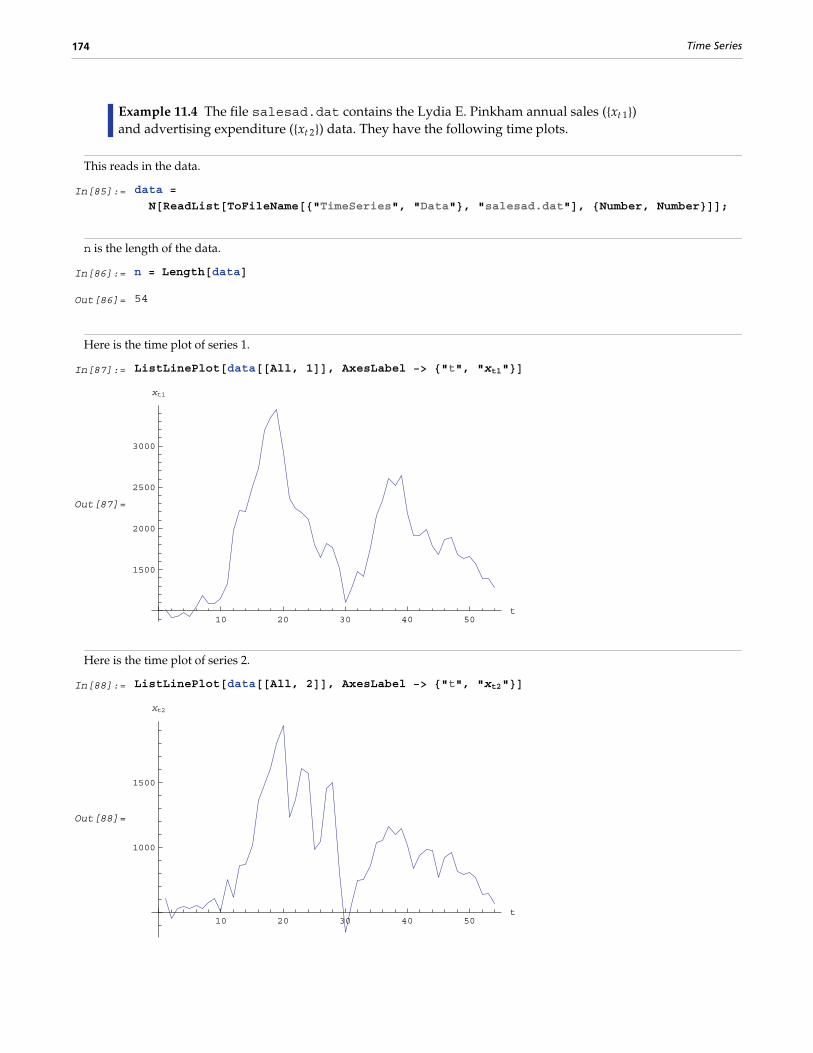
Example 11.4 The file salesad.dat contains the Lydia E. Pinkham annual sales (8xt 1<) and advertising expenditure (8xt 2<) data. They have the following time plots.
This reads in the data.
In[85]:= data =
N@ReadList@ToFileName@8"TimeSeries", "Data"<, "salesad.dat"D, 8Number, Number<DD;n is the length of the data.
In[86]:= n = Length@dataDOut[86]= 54
Here is the time plot of series 1.
In[87]:= ListLinePlot@data@@All, 1DD, AxesLabel −> 8"t", "xt1"<D
Out[87]=
10 20 30 40 50t
1500
2000
2500
3000
xt1
Here is the time plot of series 2.
In[88]:= ListLinePlot@data@@All, 2DD, AxesLabel −> 8"t", "xt2"<D
Out[88]=
10 20 30 40 50t
1000
1500
xt2
174 Time Series

Since we do not see a convincing systematic trend, we transform the series to zero-mean by simply subtractingthe sample mean of the series.
This is the sample mean.
In[89]:= μ = Mean@dataDOut[89]= 81829.48, 934.519<
The mean is subtracted.
In[90]:= data0 = H − μL & ê@ data;
We use the Hannan-Rissanen procedure to select preliminary models.
In[91]:= models = HannanRissanenEstimate@data0, 5, 5, 5, 6D;Inverse::luc : Result for Inverse of badly conditioned matrix991.60792 ×107, 9 , 6 =, 97.98007 ×10⁶, 9 , 6 =, 7 , 8 1 <, 6 =
may contain significant numerical errors.
This allows us to see the orders of each selected model.
In[92]:= If@Head@ D === ARMAModel,Head@ D@Length@ @@1DDD, Length@ @@2DDDD, Head@ D@Length@ @@1DDDDD & ê@ models
Out[92]= 8ARModel@1D, ARModel@3D, ARMAModel@2, 1D, ARMAModel@1, 1D, ARModel@2D, ARMAModel@1, 2D<This gives their AIC values.
In[93]:= AIC@ , 54D & ê@ models
Out[93]= 820.9673, 20.7213, 20.7263, 20.9195, 20.9213, 20.842<Since the second (AR(3)) and third (ARMA(2, 1)) models have the smallest AIC values, we choose them to beour preliminary models. The conditional maximum likelihood method gives the following parameter estimates.
This gives the conditional maximum likelihood estimate.
In[94]:= 8ar3, arma21< = ConditionalMLEstimate@data0, D & ê@ Take@models, 82, 3<DOut[94]= [email protected], −0.162305<, 80.585785, 0.51886<<,88−0.30868, −0.280303<, 8−0.536465, −0.339297<<,880.00254444, 0.100379<, 80.264333, 0.273705<<<,8836490.3, 14660.1<, 814660.1, 23427.2<<D,
[email protected], −0.197557<, 8−0.597596, 0.77419<<,88−0.180859, −0.235908<, 80.924474, −0.630635<<<,8880.0445299, 0.0728988<, 81.22388, −0.360301<<<,8835762.5, 15279.6<, 815279.6, 23141.6<<D<
1.11: Examples of Analysis of Time Series 175

In fact, it is unnecessary to further estimate the parameters of AR(3) model as we have done above, since theHannan-Rissanen method and the conditional maximum likelihood method give identical parameter estimatesfor an AR(p) model. The reader should convince himself/herself of this.
This gives the AIC values.
In[95]:= AIC@ , 54D & ê@ %
Out[95]= 820.7213, 20.6471<Since AR(2, 1) model has a lower AIC value, we choose it as our model and plot the residual correlation func-tions and cross-correlation function.
This gives the residuals.
In[96]:= res = Residual@data0, arma21D;This calculates the correlation function of the residuals.
In[97]:= corr = CorrelationFunction@res, 12D;Here is the plot of the residual correlation function for series 1.
In[98]:= plotcorr@ @@1, 1DD & ê@ corr, Joined −> True, AxesLabel −> 8"k", "ρ11HkL"<D
Out[98]=
2 4 6 8 10 12k
−0.1
0.1
0.2
0.3
0.4
ρ11HkL
176 Time Series

Here is the plot of the residual correlation function for series 2.
In[99]:= plotcorr@ @@2, 2DD & ê@ corr, Joined −> True, AxesLabel −> 8"k", "ρ22HkL"<D
Out[99]=
2 4 6 8 10 12k
−0.1
0.1
0.2
0.3
0.4
0.5
ρ22HkL
This is the plot of the residual cross-correlation function.
In[100]:=
plotcorr@ @@1, 2DD & ê@ corr, Joined −> True, AxesLabel −> 8"k", "ρ12HkL"<DOut[100]=
2 4 6 8 10 12k
0.1
0.2
0.3
ρ12HkL
The residual correlation functions resemble those of white noise (since 2 ë 54 º 0.272). The model also passesthe portmanteau test.
This gives Q12.
In[101]:=
PortmanteauStatistic@res, 12DOut[101]=
38.9857
1.11: Examples of Analysis of Time Series 177

The model passes the test.
In[102]:=
Quantile@ChiSquareDistribution@36D, 0.95DOut[102]=
50.9985
This calculates the inverse of the information matrix.
In[103]:=
Inverse@InformationMatrix@data0, arma21DD;Here are the standard errors of estimated parameters.
In[104]:=
Sqrt@Diagonal@%D ê nDOut[104]=80.300932, 0.214004, 0.430938, 0.389822, 0.30574, 0.192439,
0.446683, 0.337158, 0.345876, 0.225473, 0.449526, 0.425352<These are the standard errors of 8HF1L11, HF1L12, HF1L21, … , HQ1L22<. We can display the estimated parameters andtheir standard errors together using TableForm.
The parameters are displayed along with their standard errors.
In[105]:=
TableForm@Transpose@88Phi@1D, Phi@2D, Theta@1D<,Flatten@8arma21@@1DD, arma21@@2DD<, 1D, Partition@Partition@%, 2D, 2D<DD
Out[105]//TableForm=
Phi@1D 1.27204 −0.197557−0.597596 0.77419
0.300932 0.2140040.430938 0.389822
Phi@2D −0.180859 −0.2359080.924474 −0.630635
0.30574 0.1924390.446683 0.337158
Theta@1D 0.0445299 0.07289881.22388 −0.360301
0.345876 0.2254730.449526 0.425352
Again we can set several elements of the parameter matrices to zero. We find the forecast values for the next 15time steps.
This gives the predicted values.
In[106]:=
BestLinearPredictor@data0, arma21, 15D@@1DD;The mean is added to the prediction.
In[107]:=
xhat = + μ & ê@ %;
178 Time Series

This plots series 1 and the next 15 predicted values.
In[108]:=
plotdata@data@@All, 1DD, xhat@@All, 1DD, AxesLabel −> 8"t", "x1t"<DOut[108]=
10 20 30 40 50 60 70t
1500
2000
2500
3000
x1t
This plots series 2 and the next 15 predicted values.
In[109]:=
plotdata@data@@All, 2DD, xhat@@All, 2DD, AxesLabel −> 8"t", "x2t"<DOut[109]=
10 20 30 40 50 60 70t
1000
1500
x2t
1.11: Examples of Analysis of Time Series 179

Part 2.Summary of Time Series Functions

2.1 Model PropertiesA discrete time series consists of a set of observations 8x1, x2, … , xt, … < of some phenomenon, taken at equallyspaced time intervals. (We assume that xt is real.) The main purpose of time series analysis is to understand theunderlying mechanism that generates the observed data and, in turn, to forecast future values. We assume thatthe generating mechanism is probabilistic and that the observed series 8x1, x2, … , xt, … < is a realization of astochastic process 8X1, X2, … , Xt, … <. Typically, the process is assumed to be stationary and described by aclass of linear models called autoregressive moving average (ARMA) models.
An ARMA model of orders p and q (ARMA(p, q)) is defined by
Xt - f1 Xt-1 - f2 Xt-2 - … - fp Xt-p = Zt + q1 Zt-1 + q2 Zt-2 + … + qq Zt-q
where 8fi< and 8qi< are the coefficients of the autoregressive (AR) and moving average (MA) parts, respectively,and 8Zt< is white noise with mean zero and variance s2. (We assume Zt is normally distributed.) Using thebackward shift operator B defined by Bj Xt = Xt-j, the ARMA(p, q) model above can be written as
fHBL Xt = qHBL Zt
where fHBL = 1 - f1 B - f2 B2 - … - fp Bp and qHBL = 1 + q1 B + q2 B2 + … + qq Bq. We assume that the polynomialsfHxL and qHxL have no common zeros. When Xt is a vector, we have a multivariate or vector ARMA model; inthis case, the AR and MA coefficients are matrices and the noise covariance is also a matrix denoted by S. Whenall the zeros of the polynomial fHxL (or its determinant in the multivariate case) are outside the unit circle, themodel is said to be stationary and the ARMA(p, q) model can be expanded formally as an MA(¶) model(Xt = ⁄i=0
¶ yi Zt-i). Similarly, if the zeros of qHxL are all outside the unit circle, the ARMA(p, q) model is said to be
invertible and can be expanded as an AR(¶) model.
Autoregressive integrated moving average (ARIMA) models are used to model a special class of nonstationaryseries. An ARIMA(p, d, q) (d non-negative integer) model is defined by H1 - BLd fHBL Xt = qHBL Zt.
Seasonal models are used to incorporate cyclic components in models. A class of commonly encountered sea-sonal models is that of seasonal ARIMA (SARIMA) models. A SARIMA(p, d, q)(P, D, Q)s model (d and D arenon-negative integers and s is the period) is defined by H1 - BLd H1 - BsLD fHBL FHBsL Xt = qHBL QHBsL Zt
where FHxL and QHxL are polynomials that describe the seasonal part of the process.
The commonly used time series models are represented in this package by objects of the generic formmodel[param1, param2, …]. Each of these objects serves to specify a particular model and does not itselfevaluate to anything. They can be entered as arguments of time series functions as well as generated as output.

ARModelAphilist, s2E ARHpL model with p AR coefficients in philist and normallydistributed noise with variance s2
MAModelAthetalist, s2E MAHqL model with q MA coefficients in thetalist and normallydistributed noise with variance s2
ARMAModelAphilist, thetalist, s2E ARMAHp, qL model with p AR and q MA coefficients in philistand thetalist, respectively, and normally distributed noise withvariance s2
ARIMAModelAd, philist, thetalist, s2E ARIMAHp, d, qL model with p AR and q MA coefficients inphilist and thetalist, respectively, and normally distributednoise with variance s2
SARIMAModelA9d, D=, s, philist,Philist, thetalist, Thetalist, s2E SARIMAHp, d, qLHP, D, QLs model with p regular and P seasonal
AR coefficients in philist and Philist and q regular and Qseasonal MA coefficients in thetalist and Thetalist, respectively,and normally distributed noise with variance s2
Time series models.
Here, when model is used as a Mathematica function argument it means the model object defined above. Thenotation philist denotes a list of AR coefficients 9f1, f2, … , fp=, thetalist specifies a list of MA coefficients9q1, q2, … , qq=, and so on. The noise is zero-mean Gaussian white noise, and its variance or covariance matrixwill be called the noise parameter. d (or D) is the order of differencing, and s is the seasonal period. To extractany of these arguments from a model, we can use the function Part or one of the following functions.
ARCoefficientsAmodelE extract the AR coefficients of model
MACoefficientsAmodelE extract the MA coefficients of model
SeasonalARCoefficientsAmodelE extract the seasonal AR coefficients of model
SeasonalMACoefficientsAmodelE extract the seasonal MA coefficients of model
SeasonalPeriodAmodelE extract the seasonal period of model
DifferencingOrderAmodelE extract the differencing order of model
NoiseParameterAmodelE extract the noise parameter of model
Functions extracting the parameters of time series models.
All of the functions in this package with the exception of AsymptoticCovariance and the functions analyz-ing ARCH models work for both univariate and multivariate cases, although some are illustrated using exam-ples of univariate series only.
This loads the package.
In[1]:= Needs@"TimeSeries`TimeSeries`"D
182 Time Series

ARMAModel[{0.5, -0.2}, {0.7}, 0.8] represents the ARMA(2, 1) model Xt - 0.5 Xt-1 + 0.2 Xt-2 = Zt + 0.7 Zt-1 with noise variance 0.8. Note that it does not evaluate to anything.
In[2]:= [email protected], −0.2<, 80.7<, 0.8DOut[2]= [email protected], −0.2<, 80.7<, 0.8D
We can extract the MA coefficient using MACoefficients.
In[3]:= MACoefficients@%DOut[3]= 80.7<
We can also use the function Part to extract the argument.
In[4]:= %%@@2DDOut[4]= 80.7<
This is a SARIMA(2, 2, 1)(1, 3, 0)4 model. Note that the absence of the seasonal MA part is represented by thetalist = 8 < (or thetalist = 80<).
In[5]:= SARIMAModel@82, 3<, 4, 80.4, 0.1<, 8−0.5<, 80.8<, 8<, 1DOut[5]= SARIMAModel@82, 3<, 4, 80.4, 0.1<, 8−0.5<, 80.8<, 8<, 1D
This is how we get the differencing orders of both the seasonal and ordinary parts.
In[6]:= DifferencingOrder@%DOut[6]= 82, 3<ToARModelAmodel, nE give the ARHnL model that is the order n truncation of the
ARH¶L expansion of model
ToMAModelAmodel, nE give the MAHnL model that is the order n truncation of theMAH¶L expansion of model
ToARMAModelAmodelE convert an ARIMA or a SARIMA model to an ARMA model
Conversions of time series models.
This computes the first four coefficients in the expansion of an AR(1) model as an MA(¶) model and returns the correspond-ing MA(4) model.
In[7]:= ToMAModelAARModelA8φ1<, σ2E, 4EOut[7]= MAModelA9φ1, φ1
2, φ13, φ1
4=, σ2E
2.1: Model Properties 183

The first four coefficients in the expansion of an ARMA(1, 1) model as an AR(¶) model are calculated and the correspond-ing AR(4) model is returned.
In[8]:= ToARModelAARMAModelA8φ1<, 8θ1<, σ2E, 4EOut[8]= ARModelA9θ1 + φ1, θ1 H−θ1 − φ1L, −θ1
2 H−θ1 − φ1L, θ13 H−θ1 − φ1L=, σ2E
This computes the first three coefficients in the expansion of a vector AR(2) model as an MA(¶) model and returns the corresponding vector MA(3) model.
In[9]:= ToMAModel@[email protected], −0.3<, 80.2, −0.7<<, 880.1, 0.7<, 80.3, −0.8<<<, 881, 0<, 80, 1<<D, 3DOut[9]= [email protected], −0.3<, 80.2, −0.7<<, 880.08, 0.85<, 80.2, −0.37<<,880.116, −0.239<, 8−0.224, 0.899<<<, 881, 0<, 80, 1<<D
This converts an ARIMA(2, 2, 1) into the equivalent ARMA(4, 1) model.
In[10]:= ToARMAModel@ARIMAModel@2, 80.3, 0.9<, 81.2<, 1DDOut[10]= [email protected], −0.7, −1.5, 0.9<, 81.2<, 1D
This converts a SARIMAH1, 2, 1L H1, 1, 1L2 model into the equivalent ARMA(7, 3) model.
In[11]:= ToARMAModel@SARIMAModel@82, 1<, 2, 80.5<, 8−0.7<, 80.4<, 80.3<, 1DDOut[11]= [email protected], −1.7, −0.25, 1.3, −1.9, 1.4, −0.35<, 80.4, 0.3, 0.12<, 1DGiven a model, its covariance function and correlation function can be calculated. For a univariate zero-mean,stationary process, the covariance function at lag h is defined by gHhL = EHXt+h XtL (E denotes the expectation);the correlation function, by rHhL = gHhL ê g H0L. For a multivariate process, the matrix covariance function isdefined by GHhL = EIXt+h Xt
£M (X£ denotes the transpose of X), and the matrix correlation function at lag h, RHhL, isgiven by RHHhLLi j = ri jHhL = gi jHhL í gi iH0L gj jH0L where gi jHhL = GHHhLLi j. Another useful function is the partial
correlation function. The partial correlation function at lag k, fk,k, is defined to be the correlation between Xt+k
and Xt with all intervening variables fixed. The power spectrum of a univariate ARMA(p, q) process is given bys2
2 p °qIe-i wM•2 í °fIe-i wM•2, and for a multivariate process the power spectrum is 1
2 p f-1Ie-i wM qIe-i wM Sq£Iei wM f£-1Iei wM.
184 Time Series

StationaryQAmodelE give True if model is stationary, False otherwise
StationaryQAphilistE give True if the model with its AR coefficients in philist isstationary, False otherwise
InvertibleQAmodelE give True if model is invertible, False otherwise
InvertibleQAthetalistE give True if the model with its MA coefficients in thetalist isinvertible, False otherwise
CovarianceFunctionAmodel, nE give the covariance function of model up to lag n
CorrelationFunctionAmodel, nE give the correlation function of model up to lag n
PartialCorrelationFunctionAmodel, nE give the partial correlation function of model up to lag n
SpectrumAmodel, wE give the power spectrum of model as a function of w
Properties of time series models.
This time series model has the AR polynomial fHxL = 1 - 0.5 x + 0.2 x2 - 1.5 x3. fHxL = 0 has roots inside the unit circle, so the process is not stationary.
In[12]:= StationaryQ@[email protected], −0.2, 1.5<, 80.2<, 1DDOut[12]= False
We can also just enter the AR coefficients to check stationarity.
In[13]:= [email protected], −0.2, 1.5<DOut[13]= False
These vector AR coefficients indicate a stationary process. The noise covariance can be omitted as we have done here since it is irrelevant for determining stationarity.
In[14]:= StationaryQ@[email protected], −0.3<, 80.2, −0.7<<, 880.1, 0.7<, 80.3, −0.8<<<DDOut[14]= True
A given time series model has the MA polynomial qHxL = 1 + 0.3 x - 0.1 x2. The roots of qHxL = 0 are all outside the unit circle, so the process is invertible.
In[15]:= InvertibleQ@[email protected]<, 80.3, −0.1<DDOut[15]= True
2.1: Model Properties 185

This gives the covariance function gHhL of an MA(1) model for h = 0, 1, 2, 3. Note that for an MA(q) model gHhL = 0 for
h > q.
In[16]:= CovarianceFunctionAMAModelA8θ1<, σ2E, 3EOut[16]= 9σ2 I1 + θ12M, σ2 θ1, 0, 0=
This yields the covariance function of a vector ARMA(1, 1) model up to lag 2.
In[17]:= CovarianceFunction@[email protected], −1.3<, 80.2, −0.7<<<,8880.3, 0.5<, 80.2, −0.5<<<, 881.2, 0.1<, 80.1, 0.8<<D, 2DOut[17]= 8883.90967, 1.91333<, 81.91333, 2.46403<<,88−1.29539, −2.39058<, 8−0.367393, −1.72216<<,880.218534, 1.76069<, 8−0.00190227, 0.727395<<<
The correlation function of an AR(1) model is calculated up to lag 5.
In[18]:= CorrelationFunctionAARModelA8φ1<, σ2E, 5EOut[18]= 91, φ1, φ1
2, φ13, φ1
4, φ15=
This gives the partial correlation function fk,k of an AR(2) model at lags k = 1, 2, 3, and 4. Note that the partial correlation
function starts at lag 1, and for an AR(p) process, fk,k = 0 for k > p.
In[19]:= PartialCorrelationFunction@[email protected], −0.2<, 1D, 4DOut[19]= 80.416667, −0.2, 0, 0<
Here is the power spectrum of an ARMA(1, 1) model as a function of ω.
In[20]:= Spectrum@ARMAModel@8φ1<, 8θ1<, 1D, ωDOut[20]=
1 + 2 Cos@ωD θ1 + θ122 π I1 − 2 Cos@ωD φ1 + φ12M
186 Time Series

This yields the plot of the spectrum calculated above with f1 = 0.7 and q1 = -0.2.
In[21]:= Plot@% ê. 8φ1 −> 0.7, θ1 −> −0.2<,8ω, 0, Pi<, AxesLabel −> 8"ω", "fHωL"<, PlotRange −> AllD
Out[21]=
0.5 1.0 1.5 2.0 2.5 3.0ω
0.4
0.6
0.8
1.0
fHωL
RandomSequenceAm, s2, nE generate a random sequence of length n distributed normallywith mean m and variance s2
TimeSeriesAmodel, nE generate a time series of length n from model
TimeSeriesAmodel,n, 9x-p+1, x-p+2, …, x0= E generate a time series with p given initial values
TimeSeriesAmodel,n, 9z-q+1, z-q+2, …, zn=,9x-p+1, x-p+2, …, x0= E generate a time series with a given noise sequence 8z< and
initial values 8x<Generating random sequences and time series.
Both RandomSequence and TimeSeries uses the current default random number generator. Sequencesgenerated prior to Version 6.0 of Mathematica can be obtained by using the legacy generator viaSeedRandom@Method −> LegacyD or SeedRandom[seed, Method->"Legacy"].
A sequence of 5 random numbers is generated. They are normally distributed with mean 0 and variance 1.2.
In[22]:= RandomSequence@0, 1.2, 5DOut[22]= 8−0.0561913, 0.687886, −1.96931, 1.00539, −0.363847<
This generates a sequence of 4 random vectors distributed normally with mean 80.5, 0.7< and covariance matrix 880.9, -0.2<, 8-0.2, 1.0<<. Note that we have used SeedRandom[1039] to start the random number generator with seed 1039.
In[23]:= HSeedRandom@1039D;[email protected], 0.7<, 880.9, −0.2<, 8−0.2, 1.0<<, 4DL
Out[23]= 88−0.612201, 1.21709<, 81.96981, 1.54269<,8−0.0190734, 0.737721<, 82.14867, 0.760779<<
2.1: Model Properties 187

Here is a scalar time series of length 7 generated from the ARMA(2, 1) model Xt - 0.5 Xt-1 + 0.2 Xt-2 = Zt + 0.7 Zt-1. The normally distributed noise has a mean 0 and a variance of 0.8.
In[24]:= HSeedRandom@1234D;TimeSeries@[email protected], −0.2<, 80.7<, 0.8D, 7DL
Out[24]= 80.755487, −0.12346, −0.115633, 0.825265, 0.939603, −0.0773533, −0.575972<This generates a time series 8x1, x2, … , x7< from the same model as above with given values of x-1 = -0.3, and x0 = 0.5.
In[25]:= HSeedRandom@1234D;TimeSeries@[email protected], −0.2<, 80.7<, 0.8D,
7, 8−0.3, 0.5<DLOut[25]= 81.0077, −0.188289, −0.198489, 0.796802, 0.941943, −0.0704908, −0.573008<
Here is a vector time series of length 5 generated from a vector MA(2) model. Note that the MA parameters and the noise covariance are now matrices.
In[26]:= HSeedRandom@1673D;TimeSeries@[email protected], −0.2<, 8−0.2, 0.1<<,880.7, −1.2<, 80.3, −0.2<<<, 881, 0<, 80, 1<<D, 5DL
Out[26]= 882.28449, −0.659337<, 8−0.945795, 0.0369965<,80.298284, −0.210925<, 8−0.0754738, −1.0219<, 8−0.129903, −1.41094<<This generates a scalar time series of length 8 from the SARIMA(2, 2, 2)(2, 1, 1)2 model H1 - BL2 I1 - B2M I0.2 B2 - 0.5 B + 1M I0.1 B4 - 0.3 B2 + 1M Xt = I1 + 0.6 B - 0.1 B2M I1 - 0.5 B2M Zt with noise variance 0.9.
In[27]:= HSeedRandom@1234D;TimeSeries@SARIMAModel@82, 1<, 2, 80.5, −0.2<, 80.3, −0.1<, 80.6, −0.1<, 8−0.5<, 0.9D, 8DL
Out[27]= 8−7.69176, −9.38373, −17.4059, −18.9872, −26.734, −28.3097, −36.5849, −37.9153<
188 Time Series

2.2 Analysis of ARMA Time SeriesGiven a time series, we can analyze its properties. Since many algorithms for estimating model parametersassume the data form a zero-mean, stationary process, appropriate transformations of the data are often neededto make them zero-mean and stationary. The function ListDifference does appropriate differencing onARIMA or SARIMA data. Note that all time series data should be input as a list of the form 8x1, x2, … < where xi
is a number for a scalar time series and is itself a list, xi = 8xi 1, xi 2, … , xi m<, for an m-variate time series.
ListDifferenceAdata, dE difference data d times
ListDifferenceAdata, 9d, D=, sE difference data d times with period 1 and D times with period s
Sample mean and transformations of data.
After appropriate transformations of the time series data, we can calculate the properties of the series. The
sample covariance function g` HhL for a zero-mean time series of n observations is defined to be 1n
⁄t=1n-h Xt+h Xt
£. The
sample correlation function r` HhL is the sample covariance function of the corresponding standardized series, and
the sample partial autocorrelation function is defined here as the last coefficient in a Levinson-Durbin estimate
of AR coefficients. The sample power spectrum f`HwL is the Fourier transform of the sample covariance function
f` HwL = 1
2 p ⁄k=-Hn-1Ln-1 g̀ HkL e-i k w. The smoothed spectrum f
`S using the spectral window 8WH0L, WH1L, … , WHML< is
defined to be f`S IwjM = ⁄k=-M
M W HkL f` Iwj-kM where WHkL = WH-kL, while the smoothed spectrum f`L using the lag
window 8lH0L, lH1L, … , lHML< is defined by f`L HwL = 1
2 p ⁄k=-M
M l HkL g`
HkL e-i k w where lHkL = lH-kL. CovarianceFunctionAdata, nECovarianceFunctionAdata1, data2, nE give the sample covariance function of data or the cross-
covariance function of data1 and data2 up to lag n
CorrelationFunctionAdata, nECorrelationFunctionAdata1, data2, nE give the sample correlation function of data or the cross-
correlation function of data1 and data2 up to lag n
PartialCorrelationFunctionAdata, nE give the sample partial correlation function of data up to lag n
SpectrumAdataESpectrumAdata1, data2E give the sample power spectrum of data or the cross-spectrum
of data1 and data2
SmoothedSpectrumSAspectrum, windowE give the smoothed spectrum using the spectral window
window
SmoothedSpectrumLAcov, window, wE give the smoothed spectrum as a function of w using the lag
window window
Properties of observed data.

This loads the package.
In[1]:= Needs@"TimeSeries`TimeSeries`"DThe increasing magnitude of the data indicates a nonstationary series. We know this is the case, since it is generated froman ARIMA(1, 2, 0) process. Note that since the model has no MA part, the list of the MA parameters can be specified by 8 < or by 880, 0<,80, 0<<.
In[2]:= HSeedRandom@3456D;TimeSeries@ARIMAModel@2, 8880.3, −0.1<, 80.4, 0.5<<<, 8<, 881, 0<, 80, 1<<D, 10DL
Out[2]= 88−5.09594, −4.22676<, 8−8.62944, −9.74584<, 8−9.73182, −15.3683<,8−9.95509, −21.2617<, 8−8.29291, −27.4899<, 8−7.038, −32.8041<,8−4.27451, −37.8621<, 8−1.06048, −38.8798<, 82.15982, −38.9356<, 84.74157, −38.4119<<Differencing the above time series twice yields a new series that is stationary.
In[3]:= ListDifference@%, 2DOut[3]= 882.43112, −0.103382<, 80.879105, −0.270887<,81.88546, −0.334898<, 8−0.407277, 0.914094<, 81.50858, 0.256116<,80.450541, 4.04031<, 80.00627729, 0.961922<, 8−0.638555, 0.57953<<
A SARIMA(2, 2, 0)(1, 1, 0)2 series is transformed into a stationary series by differencing.
In[4]:= HSeedRandom@123D;tseries =
TimeSeries@SARIMAModel@82, 1<, 2, 80.5, −0.2<, 80.5<, 80<, 80<, 1D, 10D;ListDifference@tseries, 82, 1<, 2DL
Out[4]= 8−0.201361, −2.67625, −1.95732, −2.6338, −1.6277, −1.1512<This generates a time series of length 200 from an AR(2) model.
In[5]:= HSeedRandom@1234D;tseries = TimeSeries@[email protected], −0.2<, 0.75D, 200D;L
This computes the sample covariance function of the above series up to lag 5.
In[6]:= CovarianceFunction@tseries, 5DOut[6]= 80.75797, 0.33583, 0.0458689, −0.0248131, −0.0930331, −0.0327725<
Here is the sample correlation function of the same series up to lag 5. Note that the correlation at lag 0 is 1.
In[7]:= CorrelationFunction@tseries, 5DOut[7]= 81., 0.443065, 0.0605154, −0.0327362, −0.12274, −0.0432372<
190 Time Series

This is the sample partial correlation function of the same series at lags 1 to 5. Note that the lag starts from 1 and not 0.
In[8]:= PartialCorrelationFunction@tseries, 5DOut[8]= 80.443065, −0.168959, 0.0138086, −0.129604, 0.0870806<
The power spectrum of the series is calculated here.
In[9]:= spec = Spectrum@tseriesD;This is the plot of the spectrum in the frequency range [0, p].
In[10]:= ListLinePlot@Transpose@8Table@2 Pi ê200 ∗ k, 8k, 0, 100<D, Take@spec, 101D<D,AxesLabel −> 8"ω", "fHωL"<D
Out[10]=
0.5 1.0 1.5 2.0 2.5 3.0ω
0.1
0.2
0.3
0.4
0.5
fHωL
This gives the smoothed spectrum using the Daniell spectral window.
In[11]:= SmoothedSpectrumS@spec, Table@1 ê 13, 87<DD;We plot the smoothed spectrum.
In[12]:= ListLinePlot@Transpose@8Table@2 Pi ê200 ∗ k, 8k, 0, 100<D, Drop@%, −99D<D,AxesLabel −> 8"ω", "fHωL"<D
Out[12]=
0.5 1.0 1.5 2.0 2.5 3.0ω
0.05
0.10
0.15
0.20
0.25
fHωL
2.2: Analysis of ARMA Time Series 191

This yields the smoothed spectrum using the Hanning lag window.
In[13]:= SmoothedSpectrumL@CovarianceFunction@tseries, 10D,[email protected] + 0.5 Cos@Pi k ê10D, 8k, 0, 10<D, ωD;
This is the plot of the smoothed spectrum.
In[14]:= Plot@%, 8ω, 0, Pi<, AxesLabel −> 8"ω", "fHωL"<D
Out[14]=
0.5 1.0 1.5 2.0 2.5 3.0ω
0.05
0.10
0.15
0.20
fHωL
We calculate the correlation function up to lag 2 from data generated from a vector MA(1) model.
In[15]:= Htseries = TimeSeries@[email protected], −0.1<, 80.4, 1.2<<<, 881, 0<, 80, 1<<D, 50D;CorrelationFunction@tseries, 2DL
Out[15]= 8881., −0.28224<, 8−0.28224, 1.<<, 880.309885, −0.300356<, 8−0.109964, 0.522227<<,880.00525678, −0.142099<, 8−0.187691, 0.000553525<<<When fitting a given set of data to a particular ARMA type of model, the orders have to be selected first. Usu-ally the sample partial correlation or sample correlation function can give an indication of the order of an AR oran MA process. An AIC or a BIC criterion is also used to select a model. The AIC criterion chooses p and q to
minimize the value of ln s̀p,q2
+ 2 Hp + qL ê n by fitting the time series of length n to an ARMA(p, q) model (here s̀p,q2
is the noise variance estimate, usually found via maximum likelihood estimation). The BIC criterion seeks to
minimize ln s̀p,q2
+ Hp + qL ln n ê n.
AICAmodel, nE give the AIC value of model fitted to data of length n
BICAmodel, nE give the BIC value of model fitted to data of length n
AIC and BIC values.
Given a model, various methods exist to fit the appropriately transformed data to it and estimate the parame-ters. HannanRissanenEstimate uses the Hannan-Rissanen procedure to both select orders and performparameter estimation. As in the long AR method, the data are first fitted to an AR(k) process, where k (less thansome given kmax) is chosen by the AIC criterion. The orders p and q are selected among all p § Min@pmax, kDand q § qmax using BIC.
192 Time Series

YuleWalkerEstimateAdata, pE give the Yule-Walker estimate of ARHpL model
LevinsonDurbinEstimateAdata, pE give the Levinson-Durbin estimate of ARHiL model for i = 1, 2,…, p
BurgEstimateAdata, pE give the Burg estimate of ARHiL model for i = 1, 2, …, p
InnovationEstimateAdata, qE give the innovation estimate of MAHiL model for i = 1, 2, …, q
LongAREstimateAdata, k, p, qE give the estimate of ARMAHp, qL model by first finding theresiduals from ARHkL process
HannanRissanenEstimateAdata, kmax, pmax, qmaxE give the estimate of the model with the lowest BIC value
HannanRissanenEstimateAdata, kmax, pmax, qmax, nE give the estimate of the n models with the lowest BIC values
Estimations of ARMA models.
This generates a vector AR(2) series.
In[16]:= HSeedRandom@123D;newseries =
TimeSeries@[email protected], −0.1<, 80.4, 0.2<<, 88−0.5, 0.1<, 8−0.2, 0.7<<<,881, 0<, 80, 1<<D, 200D;LObserve how the vector time series data are defined and input into functions below.
In[17]:= Short@newseries, 4DOut[17]//Short=882.26787, 0.019026<, 81.51063, 2.42142<, 197 , 80.844117, −0.226315<<
The Yule-Walker estimate of the coefficients of the AR(2) series and the noise variance are returned inside the object ARModel.
In[18]:= armodel = YuleWalkerEstimate@newseries, 2DOut[18]= [email protected], −0.0108376<, 80.439688, 0.218125<<,88−0.453402, −0.0190763<, 8−0.0559706, 0.712374<<<,880.962922, 0.118976<, 80.118976, 0.828492<<D
Here the AR(p) (p § 3) coefficients and noise variance are estimated using the Levinson-Durbin algorithm. Note that the
small magnitude of f3 for AR(3) indicates that p = 2 is the likely order of the process.
In[19]:= HSeedRandom@123D;tseries = TimeSeries@[email protected], −0.2<, 1D, 200D;LevinsonDurbinEstimate@tseries, 3DL
Out[19]= [email protected]<, 0.968709D, [email protected], −0.233462<, 0.91591D,[email protected], −0.188349, −0.0889921<, 0.908656D<
2.2: Analysis of ARMA Time Series 193

The same parameters are estimated using the Burg algorithm.
In[20]:= BurgEstimate@tseries, 3DOut[20]= [email protected]<, 0.971849D, [email protected], −0.227845<, 0.921397D,
[email protected], −0.1888, −0.0745929<, 0.91627D<This gives the estimate of MA(q) (q § 4) coefficients and noise variance using the innovations algorithm.
In[21]:= HSeedRandom@123D;tseries = TimeSeries@[email protected], −0.2<, 1D, 200D;InnovationEstimate@tseries, 4DL
Out[21]= [email protected]<, 1.08259D, [email protected], −0.14926<, 1.0045D,[email protected], −0.130418, −0.101435<, 1.00234D,[email protected], −0.16681, −0.0736189, −0.113278<, 0.978422D<
This estimates the same parameters using the long AR method. The data are first fitted to an AR(10) model. The residuals together with the data are fitted to an MA(2) process using regression.
In[22]:= LongAREstimate@tseries, 10, 0, 2DOut[22]= [email protected], −0.197653<, 0.905695D
Here the parameters of the ARMA(1,2) model are estimated using the long AR method.
In[23]:= HSeedRandom@123D;tseries = TimeSeries@[email protected]<, 80.2, −0.5<, 2D, 250D;LongAREstimate@tseries, 8, 1, 2DL
Out[23]= [email protected]<, 80.00710284, −0.580108<, 1.79702DThis calculates the AIC value for the model estimated above.
In[24]:= AIC@%, 250DOut[24]= 0.610128
The Hannan-Rissanen method can select the model orders as well as estimate the parameters. Often the order selection is only suggestive and it should be used in conjunction with other methods.
In[25]:= HannanRissanenEstimate@tseries, 8, 3, 3DOut[25]= [email protected]<, 80.0449159, −0.560618<, 1.80737D
Here we select three models using the Hannan-Rissanen method.
In[26]:= HannanRissanenEstimate@tseries, 8, 3, 3, 3DOut[26]= [email protected]<, 80.0449159, −0.560618<, 1.80737D,
[email protected], −0.440279<, 1.8654D,[email protected], −0.431242, −0.155303<, 1.82901D<
194 Time Series

This gives the BIC value for each model estimated above.
In[27]:= BIC@ , 250D & ê@ %
Out[27]= 80.658128, 0.667646, 0.670034<MLEstimate gives the maximum likelihood estimate of an ARMA type of model by maximizing the exactlikelihood function that is calculated using the innovations algorithm. The built-in function FindMinimum isused and the same options apply. Two sets of initial values are needed for each parameter, and they are usuallytaken from the results of various estimation methods given above. Since finding the exact maximum likelihoodestimate is generally slow, a conditional likelihood is often used. ConditionalMLEstimate gives an estimateof an ARMA model by maximizing the conditional likelihood using the Levenberg-Marquardt algorithm.
ConditionalMLEstimateAdata, pE fit an ARHpL model to data using the conditional maximumlikelihood method
ConditionalMLEstimateAdata, modelE fit model to data using the conditional maximum likelihood
method with initial values of parameters as the arguments ofmodel
MLEstimateAdata,model, 8f1, 8f11, f12<<, …E fit model to data using maximum likelihood method with initial
values of parameters 8f11,f12<, …
LogLikelihoodAdata, modelE give the logarithm of Gaussian likelihood for the given dataand model
Maximum likelihood estimations and the logarithm of Gaussian likelihood.
option name default value
MaxIterations 30 maximum number of iterations in searchingfor minimum
Option for ConditionalMLEstimate.
A vector AR(1) series of length 200 is generated.
In[28]:= HSeedRandom@1234D;TimeSeries@[email protected], −0.1<, 80.4, 0.5<<<, 881, 0<, 80, 1<<D, 200D;L
This yields the conditional maximum likelihood estimate of the parameters of a vector AR process. In the absence of an MA part, this estimate is equivalent to a least squares estimate and no initial values for parameters are needed.
In[29]:= ConditionalMLEstimate@%, 1DOut[29]= [email protected], −0.144169<, 80.379962, 0.428523<<<,880.848146, −0.0439261<, 8−0.0439261, 0.849261<<D
2.2: Analysis of ARMA Time Series 195

This gives the conditional maximum likelihood estimate of an ARMA(2,1) model. The initial parameter values (f1 = 0.4, f2 = -0.35, q1 = 0.6) have to be provided as the arguments of ARMAModel.
In[30]:= HSeedRandom@9283D;ts1 = TimeSeries@[email protected], −0.3<, 80.5<, 1D, 100D;armamodel = ConditionalMLEstimate@ts1, [email protected], −0.35<, 80.6<, 1DDL
Out[30]= [email protected], −0.342903<, 80.628324<, 0.711585DThe Hannan-Rissanen method is used to select a model. The estimated model parameters can serve as the initial values for parameters in maximum likelihood estimation.
In[31]:= HSeedRandom@9381D;tseries =
TimeSeries@[email protected], −0.7<, 8−0.2, 0.9<<<, 881, 0<, 80, 1<<D, 100D;HannanRissanenEstimate@tseries, 10, 3, 3DL
Out[31]= [email protected], −0.543006<, 8−0.0697756, 0.640399<<<,881.23301, −0.314665<, 8−0.314665, 1.40438<<DThe above result is input here for the conditional maximum likelihood estimate.
In[32]:= ConditionalMLEstimate@tseries, %DOut[32]= [email protected], −0.755129<, 8−0.180682, 0.899108<<<,880.944411, −0.0383107<, 8−0.0383107, 1.08534<<D
A SARIMA(1, 0, 1)(0, 0, 1)2 series is generated.
In[33]:= HSeedRandom@2958D;tseries = TimeSeries@SARIMAModel@80, 0<, 2, 8−0.5<, 80<, 8−0.3<, 80.8<, 1D, 50D;L
This yields the maximum likelihood estimate of the parameters of a SARIMA(1, 0, 1)(0, 0, 1)2 model. Note that the parame-ters to be estimated are entered symbolically inside model and two initial values are needed for each of them. Since the calculation of the likelihood of a univariate series is independent of the noise variance, it should not be entered in symbolic form.
In[34]:= sarima = MLEstimate@tseries, SARIMAModel@80, 0<, 2, 8φ1<, 80<, 8θ1<, 8Θ1<, 1D,8φ1, 8−0.4, −0.41<<, 8θ1, 8−0.2, −0.22<<, 8Θ1, 80.7, 0.75<<DOut[34]= SARIMAModel@80, 0<, 2, 8−0.740659<, 80<, 8−0.300039<, 80.524104<, 0.854466D
A bivariate MA(1) series is generated.
In[35]:= HSeedRandom@4567D;ts = TimeSeries@[email protected], 0.2<, 8−0.1, 0.4<<<, 881, 0<, 80, 1<<D, 50D;L
196 Time Series

For a vector ARMA series, the calculation of maximum likelihood is not independent of the covariance matrix; the covari-ance matrix has to be input as symbolic parameters.
In[36]:= MLEstimate@ts, MAModel@888t1, t2<, 8t3, t4<<<, 88w1, w2<, 8w2, w3<<D,8t1, 80.4, 0.45<<, 8t2, 80.15, 0.16<<, 8t3, 8−0.09, −0.1<<,8t4, 80.3, 0.35<<, 8w1, 81, 0.9<<, 8w2, 80, 0.01<<, 8w3, 80.9, 1<<DOut[36]= [email protected], 0.226766<, 8−0.143536, 0.281516<<<,880.743654, −0.0202879<, 8−0.0202879, 0.734156<<D
This gives the logarithm of the Gaussian likelihood.
In[37]:= LogLikelihood@ts, %DOut[37]= −35.2266
Let b = If1, f2, … , fp, q1, q2, … , qqM£ be the parameters of a stationary and invertible ARMA(p, q) model and b
`
the maximum likelihood estimator of b. Then, as n Ø ¶, we have n1ê2 Ib`
- bM fl N H0, V HbLL. For a univariateARMA model, AsymptoticCovariance[model] calculates the asymptotic covariance V from model. Thefunction InformationMatrix[data, model] gives the estimated asymptotic information matrix whose inversecan be used as the estimate for the asymptotic covariance.
AsymptoticCovarianceAmodelE give the covariance matrix V of the asymptotic distribution ofthe maximum likelihood estimators
InformationMatrixAdata, modelE give the estimated asymptotic information matrix
Asymptotic covariance and information matrix.
This gives the asymptotic covariance matrix of the estimators of an MA(3) model.
In[38]:= AsymptoticCovarianceAMAModelA8θ1, θ2, θ3<, σ2EE;The above asymptotic covariance is displayed in matrix form.
In[39]:= MatrixForm@%DOut[39]//MatrixForm=
1 − θ32 θ1 − θ2 θ3 θ2 − θ1 θ3
θ1 − θ2 θ3 1 + θ12 − θ2
2 − θ32 θ1 − θ2 θ3
θ2 − θ1 θ3 θ1 − θ2 θ3 1 − θ32
This gives the estimate of the information matrix.
In[40]:= InformationMatrix@ts1, armamodelD;
2.2: Analysis of ARMA Time Series 197

The above information matrix is displayed here.
In[41]:= MatrixForm@%DOut[41]//MatrixForm=
1.30344 0.540457 0.6503740.540457 1.30015 −0.3973780.650374 −0.397378 1.64371
There are various ways to check the adequacy of a chosen model. The residuals 8Z` t< of a fitted ARMA(p, q)
process are defined by Z`
t = q-1HBL fHBL Xt where t = 1, 2, … , n. One can infer the adequacy of a model by look-
ing at the behavior of the residuals. The portmanteau test uses the statistic Qh = n Hn + 2L ⁄i=1h r
` 2 HiL ê Hn - iL where
r` HiL is the sample correlation function of the residuals; Qh is approximately chi-squared with h - p - q degrees offreedom. Qh for an m-variate time series is similarly defined, and is approximately chi-squared withm2Hh - p - qL degrees of freedom.
ResidualAdata, modelE give the residuals of fitting model to data
PortmanteauStatisticAresidual, hE calculate the portmanteau statistic Qh from residual
Residuals and test statistic.
The adequacy of the fitted model for the earlier example is accepted at level 0.05 for h = 20 since c.952 H72L > Q.
In[42]:= Q = PortmanteauStatistic@Residual@newseries, armodelD, 20DOut[42]= 64.8689
After establishing the adequacy of a model, we can proceed to forecast future values of the series. The bestlinear predictor is defined as the linear combination of observed data points that has the minimum mean-squaredistance from the true value. BestLinearPredictor gives the exact best linear predictions and their meansquared errors using the innovations algorithm. When the option Exact is set to False the approximate bestlinear predictor is calculated. For an ARIMA or SARIMA series 8Xt< with a constant term, the prediction for
future values of 8Xt< can be obtained from the predicted values of 8Yt<, 8Y` <, where Yt = H1 - BLd H1 - BsLD Xt, usingIntegratedPredictor.
BestLinearPredictorAdata, model, nE give the prediction of model for the next n values and their
mean square errors
IntegratedPredictorAxlist, 9d, D=, s, yhatlistE give the predicted values of 8Xt< from the predicted values
yhatlist
Predicting time series.
option name default value
Exact True whether to calculate exactly
Option for BestLinearPredictor.
198 Time Series

This gives the prediction for the next three data points and their mean square errors for the vector ARMA(1, 1) process.
In[43]:= Hmodel = [email protected], −0.2<, 80.3, −0.3<<<,888−0.5, 0.2<, 80.8, 0.3<<<, 881, 0<, 80, 1<<D;tseries1 = TimeSeries@model, 20D;BestLinearPredictor@tseries1, model, 3DL
Out[43]= 9880.0878762, 1.16349<, 8−0.188761, −0.322686<, 8−0.0298433, 0.0401774<<,9991., −2.8716 ×10−9=, 9−2.8716 × 10⁻⁹, 1.==,991., 1.26535 × 10−9=, 91.26535 ×10⁻⁹, 2.21==, 881.0484, 0.0726<, 80.0726, 2.3189<<==Here is the prediction for the next four data points and their mean square errors for the previously fitted SARIMA(1, 0, 1)(0, 0, 1)2 model.
In[44]:= BestLinearPredictor@tseries, sarima, 4DOut[44]= 88−0.341681, 0.196892, −0.0795141, 0.0588928<, 80.854466, 1.7799, 3.21265, 4.27749<<
Here is the prediction for the next four data points and their mean square errors for an ARIMA(2, 2, 2) model.
In[45]:= Hmodel = ARIMAModel@2, 81, −0.5<, 80.3, 0.6<, 1D;SeedRandom@3986D;tseries = TimeSeries@model, 20D;BestLinearPredictor@tseries, model, 4, Exact −> FalseDL
Out[45]= 88−165.981, −182.705, −200.078, −217.858<, 81, 11.89, 60.89, 191.992<<
2.2: Analysis of ARMA Time Series 199

2.3 The Kalman FilterThe Kalman filter is a technique that can be used to recursively estimate unobservable quantities called statevariables, 8Xt<, from an observed time series 8Yt<. Many time series models (including the ARMA models) can becast into a state-space form given by
Yt = Gt Xt + dt + Wt
Xt = Ft Xt-1 + ct + Vt,
where 8Yt< is the time series we observe and 8Xt< is the state variable. F, G, c, and d are known matrices orvectors, and they can be dependent on time. 8Wt< and 8Vt< are independent Gaussian white noise variables withzero mean and covariance matrices E Vt Vs
£ = dt s Qt and E Wt Ws£ = dt s Rt, respectively.
Let X`
t»s be the best linear estimate of Xt and Pt»s be its mean square error, given Is, the information up to time s.
Given the initial values 9X` m+1»m, Pm+1»m=, the Kalman filter yields 9X` m+2»m+1, Pm+2»m+1, X`
m+1»m+1, Pm+1»m+1=. KalmanFilterBYt , :X
ˆt»t+1, Pt-1>, Ft+1, Gt, Qt+1, Rt, ct+1, dtF
give 9X` t+1»t, Pt+1»t, X`
t»t , Pt»t=KalmanFilterB9Ym+1, Ym+2, …, YT<, 9X` m+1»m, Pm+1»m=, F, G, Q, R, c, dE
give 99X` m+2»m+1, Pm+2»m+1, X`
m+1»m+1, Pm+1»m+1=, …,9X` T+1»T, PT+1»T, X`
T»T, PT»T== if F, G, R, c, and d are timeindependent
Kalman filtering.
Note that if any one of F, G, Q, R, c, o r d is time dependent, F, G, Q, R, c, a n d d in the input to KalmanFiltershown above should be replaced by 8Fm+2, Fm+3, …, FT+1<, 8Gm+1, Gm+2, ..., GT<, 8Qm+2, Qm+3, …, QT+1<,8Rm+1, Rm+2, ..., RT<, 8cm+2, cm+3, …, cT+1<, and 8dm+1, dm+2, ..., dT<, respectively. Note also that if c ª 0 and d ª 0,the last two arguments of KalmanFilter can be omitted.
A fixed-point Kalman smoother gives the estimated value of the state variable at t based on all the availableinformation up to T, where T > t. The idea is that as new data are made available, we can improve our estima-tion result from the Kalman filter by taking into account the additional information.
KalmanSmoothingAfilterresult, FE "smooth" the result of the Kalman filtering
Kalman smoothing.
KalmanSmoothing gives 99X` m+1»T, X`
m+2»T, …, X`
T»T=, 8Pm+1»T, Pm+2»T, …, PT»T<=. The first argument of KalmanSmoothing, filterresult, is the result of KalmanFilter, that is,99X` m+2»m+1, Pm+2»m+1, X
`m+1»m+1, Pm+1»m+1=, …, 9X` T+1»T, PT+1»T, X
`T»T, PT»T==, and F is the transition matrix in the above

state equation. If F is time dependent, the second argument of KalmanSmoothing should be8Fm+2, Fm+3, …, FT+1<. The Kalman prediction estimates the state variable Xt+h based on the information at t, It.
KalmanPredictorB:X`
t+1»t, Pt+1»t>, F, Q, c, hFgive the next h predicted values and their mean square errors
Kalman predictor.
KalmanPredictor[9X` t+1»t, Pt+1»t=, F, Q, c, h] or KalmanPredictor[9X` t+1»t, Pt+1»t=,8Ft+2, …,Ft+h<, 8Qt+2, …, Qt+h<, 8ct+2,…,ct+h<] gives the next h predicted values and their mean square errors99X` t+1»t, X`
t+2»t, …, X`
t+h…t=, 9Pt+1»t, Pt+2»t, …, Pt+h…t==. Again, the argument c can be omitted if it is always 0.
A simple structural model is the local level model. It is given by
yt = mt + et
mt = mt-1 + ht.
The model is in state-space form with F = 1, G = 1, and c = d = 0.
This loads the package.
In[1]:= Needs@"TimeSeries`TimeSeries`"DIn the state-space model given earlier, if we set F = 1, G = 1, and c = d = 0, we have a local level model. Here we generate a time series of length 30 according to the local level model with Q = 1.2 and R = 0.6.
In[2]:= HSeedRandom@354101D;eta = RandomSequence@0, 1.2, 50D;mu = Accumulate@etaD;data1 = RandomSequence@0, 0.6, 50D + mu;L
2.3: The Kalman Filter 201

This plots the series.
In[3]:= ListLinePlot@data1D
Out[3]=
10 20 30 40 50
−5
5
10
15
To start the Kalman filter iteration, initial values are needed. Here we use the so-called diffuse prior.
In[4]:= init =
Limit@Take@KalmanFilter@data1@@1DD, 80, k<, 1, 1, 1.2, 0.6D, 2D, k −> InfinityDOut[4]= 81.05868, 1.8<
We can also use the function getInit to get the initial values.
In[5]:= getInit@y_?AtomQ, F_, G_, Q_, R_, c_: 0, d_: 0D := 8 ∗Hy − dL + c, ^2 ∗R + Q< &@Fê GD;In[6]:= getInit@y_?VectorQ, F_, G_, Q_, R_, c_: 0, d_: 0D :=
Module@8m = Length@yD, invF = Inverse@FD, temp, zero, finvtemp, tempzero<,zero = Table@0, 8m<D;temp = Flatten@NestList@ .invF &, G, m − 1D, 1D;finvtemp = F.Inverse@Reverse@tempDD;tempzero = Append@Reverse@Rest@tempDD, zeroD;8finvtemp.Hy − d + If@c === 0, 0, Reverse@Accumulate@[email protected] + c,finvtemp.HOuter@Total@MapThread@Dot, 8 1, 2<DD &,
NestList@Append@Rest@ D, zeroD &, .Q & ê@ tempzero, m − 1D,NestList@Append@Rest@ D, zeroD &, tempzero, m − 1D, 1D +
R [email protected]@finvtempD + Q<DIn[7]:= init = getInit@data1@@1DD, 1, 1, 1.2, 0.6DOut[7]= 81.05868, 1.8<
This gives the result of Kalman filtering. Note that the initial values are 9X` 2»1, P2»1= and the series now starts from t = 2.
In[8]:= kf = KalmanFilter@Rest@data1D, init, 1, 1, 1.2, 0.6D;
202 Time Series

Here the form of the output of KalmanFilter is shown. It is a list of 9X` t+1»t, Pt+1»t, X`
t»t, Pt»t= for t = 2, 3, …, T, with
T = 50.
In[9]:= Short@kf, 6DOut[9]//Short=88−0.453302, 1.65, −0.453302, 0.45<,80.983304, 1.64, 0.983304, 0.44<, 46 , 816.7961, 1.63923, 16.7961, 0.43923<<
This gives the smoothed estimates of the trend and their mean square errors.
In[10]:= KalmanSmoothing@kf, 1D;Note that the output of KalmanSmoothing is a list of two lists. The first list contains X
`t»T for t = 2, 3, …, T, with T = 50
and the second list contains the corresponding mean square errors.
In[11]:= Dimensions@%DOut[11]= 82, 49<
The smoothed values are plotted here.
In[12]:= ListLinePlot@%%@@1DD, DataRange −> 82, 50<D
Out[12]=
10 20 30 40 50
5
10
15
This gives the next three predicted values and their mean square errors.
In[13]:= KalmanPredictor@Take@Last@kfD, 2D, 1, 1.2, 0, 3DOut[13]= 8816.7961, 16.7961, 16.7961<, 81.63923, 2.83923, 4.03923<<The Kalman filter can be used to calculate the likelihood function of a time series in state-space form.
LogLikelihoodAdata,init, F, G, Q, R, c, dE give the logarithm of the Gaussian likelihood of data
Log likelihood.
2.3: The Kalman Filter 203

Now the variances R and Q are to be estimated and the initial values depends on them.
In[14]:= init = getInit@data1@@1DD, 1, 1, q, rDOut[14]= 81.05868, q + r<
This gives maximum likelihood estimate of Q and R.
In[15]:= Clear@f, ifD;if = Function@Evaluate@init ê. 8q → 1, r → 2<DD;f@q_?NumericQ, r_?NumericQD := −LogLikelihood@Rest@data1D, if@q, rD, 1, 1, q, rD
In[16]:= FindMinimum@f@q, rD, 8q, 0.8, 0.9<, 8r, 0.3, 0.4<DOut[16]= 844.003, 8q → 1.65215, r → 0.302524<<
204 Time Series

2.4 Univariate ARCH and GARCH ModelsAutoregressive Conditional Heteroskedasticity (ARCH) models and Generalized Autoregressive ConditionalHeteroskedasticity (GARCH) models are used to model the changes in variance as a function of time. AGARCH(p, q) model is
Zt = nt ht
where 8nt< is an independently distributed Gaussian random sequence with zero mean and unit variance; ht isthe conditional variance of Zt conditional on all the information up to time t - 1, It-1:
E IZt2 … It-1M = ht = a0 + ‚
i=1
q
ai zt-i2 + ‚
i=1
p
bi ht-i.
When p = 0, we have an ARCH(q) model. A GARCH-in-mean (or ARCH-in-mean) model is defined by
Yt = d f HhtL + Zt.
That is, the conditional mean is also a function of conditional variance ht, where f HhL is usually h or h. AnARCH (or GARCH) regression model is
Yt = xt£.b + Zt
or
Yt = xt£.b + d f HhtL + Zt.
ARCHModelAalphalistE ARCHHqL model with the coefficients 8a0, a1,…,aq< in alphalist
GARCHModelAalphalist, betalistE GARCHHp, qL model with the coefficients 8a0, a1,…,aq< and8b1,…,bq< in alphalist and betalist, respectively
ARCHModelAalphalist, d, fE ARCH-in-mean model
GARCHModelAalphalist, betalist, d, fE GARCH-in-mean model
ARCH and GARCH models.
Note that the function f should be a symbol representing a Mathematica built-in function or a pure function.Note also these models will be referred as archmodel to differentiate them from ARMA type models.

TimeSeriesAarchmodel, nE generate a time series of length n from archmodel
TimeSeriesAarchmodel, n, initE generate a time series with given initial values init
Generating ARCH time series.
This loads the package.
In[1]:= Needs@"TimeSeries`TimeSeries`"DThis generates a GARCH time series of length 10. Note that the third argument is optional. It specifies the initial values99h-p+1, h-p+2, …, h0=, 9z-q+1, z-q+2, …, z0==, or 9z-q+1, z-q+2, …, z0= as in the case of an ARCH model.
In[2]:= HSeedRandom@4567D;TimeSeries@[email protected], 0.2<, 80.3<D, 10, 880.1<, 80.2<<DL
Out[2]= 80.273984, −0.0604305, 0.195588, −0.034382,0.269706, 0.1712, −0.00232378, −0.278077, −0.567274, 0.315893<
Here we generate an ARCH-in-mean series of length 10. Note that the function f should be a symbol representing a Mathe-matica built-in function (here Log) or a pure function.
In[3]:= HSeedRandom@3457D;TimeSeries@[email protected], 0.3<, 0.5, LogD, 10DL
Out[3]= 8−1.13392, −1.87536, −0.471234, −0.957423,−1.52742, −1.38422, −1.6642, −1.62875, −0.771731, −0.371803<
This generates the so-called AR-ARCH series. That is, the noise or error used in generating AR series is an ARCH process, with a0 = 0.02 and a1 = 0.3.
In[4]:= HSeedRandom@43658D;z = TimeSeries@[email protected], 0.3<D, 10D;data = TimeSeries@[email protected], −0.1<D, z, 80, 0<DL
Out[4]= 8−0.116087, −0.294447, −0.0515721, 0.256337,0.0973735, −0.222807, −0.0720606, 0.167836, 0.159846, −0.167463<
LogLikelihoodAdata, archmodelE give the logarithm of the Gaussian likelihood for the givendata and archmodel
LogLikelihoodAdata, archmodel, X, blistE give the logarithm of the Gaussian likelihood of an ARCH or
GARCH regression series data
LogLikelihoodAdata,archmodel, ARModelAphilistEE give the logarithm of the Gaussian likelihood of an AR-ARCH
or AR-GARCH series data
LogLikelihoodAdata,archmodel, ARModelAphilistE, mE give the logarithm of the Gaussian likelihood of an AR-ARCH
or AR-GARCH series with a constant mean m
Log likelihood for ARCH series.
206 Time Series
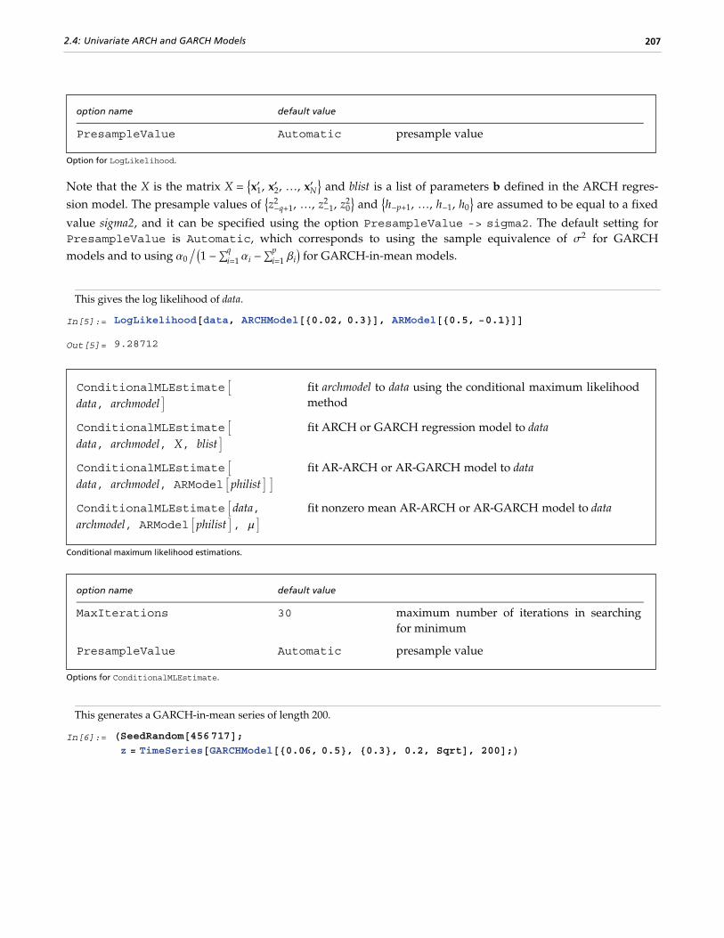
option name default value
PresampleValue Automatic presample value
Option for LogLikelihood.
Note that the X is the matrix X = 9x1£ , x2
£ , …, xN£ = and blist is a list of parameters b defined in the ARCH regres-
sion model. The presample values of 9z-q+12 , …, z-1
2 , z02= and 9h-p+1, …, h-1, h0= are assumed to be equal to a fixed
value sigma2, and it can be specified using the option PresampleValue -> sigma2. The default setting forPresampleValue is Automatic, which corresponds to using the sample equivalence of s2 for GARCHmodels and to using a0 ë I1 - ⁄i=1
qai - ⁄i=1
pbiM for GARCH-in-mean models.
This gives the log likelihood of data.
In[5]:= LogLikelihood@data, [email protected], 0.3<D, [email protected], −0.1<DDOut[5]= 9.28712
ConditionalMLEstimateAdata, archmodelE fit archmodel to data using the conditional maximum likelihood
method
ConditionalMLEstimateAdata, archmodel, X, blistE fit ARCH or GARCH regression model to data
ConditionalMLEstimateAdata, archmodel, ARModelAphilistEE fit AR-ARCH or AR-GARCH model to data
ConditionalMLEstimateAdata,archmodel, ARModelAphilistE, mE fit nonzero mean AR-ARCH or AR-GARCH model to data
Conditional maximum likelihood estimations.
option name default value
MaxIterations 30 maximum number of iterations in searchingfor minimum
PresampleValue Automatic presample value
Options for ConditionalMLEstimate.
This generates a GARCH-in-mean series of length 200.
In[6]:= HSeedRandom@456717D;z = TimeSeries@[email protected], 0.5<, 80.3<, 0.2, SqrtD, 200D;L
2.4: Univariate ARCH and GARCH Models 207

ConditionalMLEstimate is used to estimate the model parameters. Note that the output contains the estimated model and the root mean square errors of the estimated parameters.
In[7]:= ConditionalMLEstimate@z, [email protected], 0.4<, 80.3<, 0.1, SqrtDDOut[7]= [email protected], 0.668799<, 8−0.029961<, 0.270006, SqrtD,880.0240911, 0.177117<, 80.0554242<, 0.0554242<<
We generate an AR-ARCH series of length 50.
In[8]:= HSeedRandom@4561D;z = TimeSeries@[email protected], 0.5<D, 50D;data = TimeSeries@ARModel@8−0.7<D, zD;L
This gives the conditional maximum likelihood estimate of the model parameters and their corresponding root mean square errors.
In[9]:= ConditionalMLEstimate@data, [email protected], 0.4<D, ARModel@8−0.5<DDOut[9]= [email protected], 0.299001<D, ARModel@8−0.780304<D<,880.00210545, 0.255393<, 80.149147<<<
Note that we can also first estimate the parameter of the AR model.
In[10]:= ConditionalMLEstimate@data, 1DOut[10]= ARModel@8−0.723085<, 0.0110195D
Then we estimate the ARCH parameters from the residuals. The two estimates give comparable results.
In[11]:= ConditionalMLEstimate@Residual@data, %D, [email protected], 0.4<DDOut[11]= [email protected], 0.248135<D, 80.00208182, 0.232919<<The Lagrange multiplier (LM) test is commonly used to test for the existence of ARCH. The null hypothesis isno ARCH, that is, a1 = a2 = ∫ = aq = 0 and the LM statistic has a cq
2 distribution asymptotically under the null
hypothesis.
LMStatisticAdata, archmodelE calculate LM statistic with estimated parameters under thenull inside archmodel
LMStatisticAdata, archmodel, X, blistE calculate LM statistic of an ARCH or GARCH regression series
LMStatisticAdata,archmodel, ARModelAphilistEE calculate LM statistic of an AR-ARCH or AR-GARCH series
LMStatisticAdata,archmodel, ARModelAphilistE, mE calculate LM statistic of an AR-ARCH or AR-GARCH series
with nonzero mean m
LM statistic.
208 Time Series

option name default value
PresampleValue Automatic presample value
Option for LMStatistic.
To test the existence of ARCH using the LM test, we need to estimate the parameters under the null hypothesis. Note that the null hypothesis is no ARCH, that is, a pure AR(1) model.
In[12]:= ConditionalMLEstimate@data, [email protected]<D, ARModel@8−0.5<D, MaxIterations −> 100DOut[12]= [email protected]<D, ARModel@8−0.72387<D<, 880.00184937<, 80.123171<<<
This is the alternative model with the parameters estimated under the null hypothesis. Note that a1 = 0 is inserted.
In[13]:= MapAt@Append@ , 0D &, %@@1DD, 81, 1<DOut[13]= [email protected], 0<D, ARModel@8−0.72387<D<
This gives the LM statistic.
In[14]:= LMStatistic@data, Sequence @@ %DOut[14]= 1.39372
Since this number is larger than the the above LM statistic, the null hypothesis is accepted.
In[15]:= Quantile@ChiSquareDistribution@1D, 0.95DOut[15]= 3.84146
2.4: Univariate ARCH and GARCH Models 209

References1 Berndt, E. K., Hall, B. H., Hall, R. E., and Hausman, J. A. (1974), Estimation and inference in nonlinear struc-tural models, Annals of Economic and Social Measurement, 3, 653–665.
2 Bollerslev, T. (1986), Generalized autoregressive conditional heteroskedasticity, Journal of Econometrics, 31,307–327.
3 Box, G. E. P. and Jenkins, G. M. (1970), Time Series Analysis: Forecasting and Control, Holden-Day, San Francisco.
4 Brockwell, P. J. and Davis, R. A. (1987), Time Series: Theory and Methods, Springer-Verlag, New York.
5 Campbell, M. J. and Walker A. M. (1977), A survey of statistical work on the Mackenzie River series of annualCanadian lynx trappings for the years 1821–1934 and a new analysis, Journal of the Royal Statistical Society, SeriesA, 140, 411–431.
6 Domowitz, I. and Hakkio, C. S. (1985), Conditional variance and the risk premium in the foreign exchangemarket, Journal of International Economics, 19, 47–66.
7 Engle, R. F. (1982), Autoregressive conditional heteroscedasticity with estimates of the variance of UnitedKingdom inflation, Econometrica, 50, No. 4, 987–1007.
8 Engle, R. F., Lilien, D. M., and Robins, R. P. (1987), Estimating time varying risk premia in the term structure:the ARCH-M Model, Econometrica, 55, No. 2, 391–407.
9 Godolphin, E. J. and Unwin, J. M. (1983), Evaluation of the covariance matrix for the maximum likelihoodestimator of a Gaussian autoregressive moving average process, Biometrika 70, 279–284.
10 Granger, C. W. J. and Newbold, P. (1986), Forecasting Economic Time Series, Academic Press, New York.
11 Harvey, A. C. (1981), Time Series Models, Philip Allan, Oxford.
12 Harvey, A. C. (1989), Forecasting, Structural Time Series Models and the Kalman Filter, Cambridge UniversityPress, Cambridge.
13 Jones, R. H. (1978), Multivariate autoregression estimation using residuals, Applied Time Series Analysis (ed.D. F. Findley), Academic Press, New York, 139–147.
14 Kendall, M. and Ord, J. K. (1990), Time Series, 3rd ed., Edward Arnold, London.
15 Morettin, P. A. (1984), The Levinson algorithm and its applications in time series analysis, InternationalStatistical Review, 52, 83–92.
16 Priestley, M. B. ( 1981), Spectral Analysis and Time Series, Vols. 1 and 2, Academic Press, New York.
17 Reinsel, G. C. (1993), Elements of Multivariate Time Series Analysis, Springer-Verlag, New York.
18 Wilson, G. T. (1973), The Estimation of Parameters in Multivariate Time Series Models, Journal of the RoyalStatistical Society, Series B, 35, 76–85.