1 fully physical, time-dependent thermal modelling of...
TRANSCRIPT
1
Fully physical, time-dependent thermal modelling of complex3-dimensional systems for device and circuit level electro-thermal CAD
W. Batty×+, C. E. Christoffersen∗, S. David×, A. J. Panks×,R. G. Johnson×, C. M. Snowden× and M. B. Steer∗,
×Institute of Microwaves and Photonics, ∗Department of Electrical and Computer Engineering,School of Electronic and Electrical Engineering, North Carolina State University (NCSU),
University of Leeds, Leeds LS2 9JT, UK. Raleigh, NC 27695-7914, USA.+Contact author:
tel. +44 113 2332089, fax +44 113 2332032, e-mail [email protected]
Abstract— An original spectral domain decomposition ap-proach, to solution of the time-dependent heat diffusionequation in complex volumes, is introduced. Its applica-tion to device and circuit level electro-thermal simulationon CAD timescales is outlined. The first full treatment incoupled electro-thermal CAD, of thermal non linearity dueto temperature dependent diffusivity, is described. Origi-nal thermal solutions are presented in the form of analyti-cally exact thermal impedance matrix expressions for ther-mal subsystems. These include time domain expressionsfor MMICs, found to be rapidly convergent for all times,and original double Fourier series solutions for the case ofarbitrarily distributed volume heat sources and sinks, con-structed without the use of Green’s function techniques.The time-independent thermal resistance matrix approachis illustrated by a fully physical, coupled electro-thermaldevice study of the interaction of substrate thickness andsurface convection in power HEMTs. The thermal time-dependent implementation is illustrated by circuit leveltransient simulation of a 3×3 MMIC amplifier array.
I. Introduction
Solutions of the heat diffusion equation for complex 3-dimensional systems are commonly based on finite volume,finite element, finite difference or boundary element meth-ods. All of these approaches require construction of a vol-ume or surface mesh. They are computationally inten-sive and therefore generally unsuitable for direct imple-mentation in the necessarily iterative solution of intrin-sically non linear coupled electro-thermal problems. Inthis paper, a new approach is presented to the solution ofthe time-dependent heat diffusion equation in complex 3-dimensional volumes. Generically, this approach is a spec-tral domain decomposition technique [1]. Simple compos-ite systems have been treated previously by the UnsteadySurface Element (USE) method of Beck et al., [2], andthis approach has the advantage that it only discretises in-terfaces between subsystems. Like the USE method, theapproach presented here discretises only interfaces (andheating elements). It constructs solutions for thermal sub-volumes which are fully analytical, with development ofdouble Fourier series solutions for thermal subvolumes byexplicit construction of series expansion coefficients. Thusit differs from semi-analytical Fourier approaches for sim-ple rectangular multilayers [3], based on collocation orfunction sampling, which require numerical manipulationsuch as DFT-FFT to generate expansion coefficients. Assolutions for subvolumes are fully analytical, no volumeor surface mesh is required. Global solutions for complexvolumes are constructed by matching of temperature andflux at subvolume interfaces. Such solutions are applicablefor describing complex structures, from metallised, multi-gate power FETs, through MMICs and MCMs, upto cir-cuit board level. A particular intended application is the
treatment of MMIC arrays for spatial power combining atmillimeter wavelengths.
Importantly, this modular thermal solution is con-structed to be compatible with coupled electro-thermaldevice and circuit simulation on CAD timescales. Thisis achieved by formulating the analytically exact subsys-tem solutions in terms of thermal impedance matrices.These thermal impedance matrices describe explicitly, onlythe temperature variation with time, in the vicinity ofthe power dissipating and interface regions required forcoupling of the electrical and thermal problems. No re-dundant temperature information is generated on the sur-face or in the body of the subsystem volumes. As theseminimal thermal solutions are generated analytically, thethermal impedance matrices are all precomputed, priorto the coupled electro-thermal simulation, purely fromstructural information. Thermal updates in the coupledelectro-thermal problem are therefore rapid. However,each thermal impedance matrix corresponds to full ana-lytical solution of the heat diffusion equation. Thus, oncepower dissipation of active elements has been obtained self-consistently, by coupled electro-thermal simulation, de-scription of temperature variation at any instant, at anypoint within the body, or on the surface, of the complex3-dimensional volume, can be obtained essentially exactly,for model validation by comparison against thermal mea-surements.
Fully coupled device level simulation can be be imple-mented by combination of this thermal impedance ma-trix model with any thermally self-consistent device model.If the device model includes self-heating effects, then theglobal thermal impedance matrix will provide an accurate,CAD timescale, description of mutual thermal interactionbetween power dissipating elements, however complex thethermal system. The matrix form of the analytical ther-mal solution for subsystems, means that global thermalimpedance matrices can be expressed explicitly in termsof simple manipulations on subsystem matrices. Coupledelectro-thermal solution is achieved by iterative solutionof the electrical and thermal problems, with thermal up-dates provided by small matrix multiplications, and ther-mal non linearity transferred to the already non linear ac-tive device model. Fully physical, coupled electro-thermalsimulations for the thermal time-independent and time-dependent cases, have been described by the authors previ-ously [4]–[7]. These were based on coupling of the thermalmodel presented here, to the quasi-2-dimensional LeedsPhysical Model of MESFETs and HEMTs [8]–[11].
Circuit implementation of this thermal solution, exploitsthe ability of network based microwave circuit simulatorsto describe multiport non linear elements in the time do-main, and to treat distributed EM systems in terms ofmultiport network parameters [12]. The thermal solutionmakes use of the close analogy between distributed EM and
2
thermal systems. The magnetic vector potential equationin frequency space, is just the Helmholtz equation, as is thetime-dependent heat diffusion equation in Laplace trans-form s-space (complex frequency space), after appropriatetransformation of thermal non linearity. Double Fourierseries thermal solutions resemble analytical EM Green’sfunction solutions (and the same series acceleration tech-niques can be used in each case). Most importantly, com-plex EM systems are treated by segmentation [13] and cas-cading of subsystem solutions by use of network parametermatrices. The transformed (initially non linear) thermalproblem is therefore immediately compatible with networkbased microwave circuit simulation engines, by interpreta-tion of thermal impedance matrices, for distributed ther-mal subsystems, in terms of generalised multiport networkparameters. Analytical, s-space solution for thermal sub-systems, means that no numerical identification of thermalnetworks, such as that provided by the NID method [14],is required. It also means that each thermal subsystem canbe described in either the time domain or in the frequencydomain. In the time domain, the thermal subsystem istreated as a non linear multi-port element, which readilyallows non linear matching of transformed temperaturesat thermal subsystem interfaces [4], [5]. In the frequencydomain, the thermal subsystem is represented by a matrixof complex phasors inserted into the modified nodal ad-mittance matrix (MNAM) for the microwave system, andthermal non linearity is again transferred to the alreadynon linear active device model. This gives coupled electro-thermal harmonic balance and transient solutions on CADtimescales. Coupled electro-thermal circuit level CAD gen-erally requires thermal model reduction, e.g., [15]–[17].Rapidly convergent, fully analytical and minimal thermalimpedance matrix expressions, in both the time and fre-quency domains, mean that no reduced, lumped element,RC network description, is required in the multiport net-work parameter approach. Analytical expressions for themultiport network parameters of all thermal subvolumesmeans that no distinct thermal simulator, separate fromthe coupled electro-thermal simulation engine, is requiredto characterise the complex thermal system. Such simu-lations have been described by the authors in [18] whichoutlines the coupling of the thermal model to microwavecircuit simulator Transim (NCSU) [19].
A key aspect of the thermal solution presented here, isapplication of a generalised ‘radiation’ boundary condition,on the top and bottom surfaces of all thermal subvolumes,in the analytical subsystem solutions. This boundary con-dition allows analytical subsystem solutions with interfacediscretisation, and construction of global thermal solutionsby vertical matching of temperatures and fluxes at subsys-tem interfaces. The boundary condition also allows inte-gral treatment of surface radiation and convection. Oneaim of this paper is to present explicit analytical solutionsfor thermal subsystem impedance matrices, allowing globalsolution for complex systems. Generation of such solu-tions requires treatment of thermal non linearity inherentin temperature dependence of material parameters. Anoriginal treatment of this non linearity, for device and cir-cuit level electro-thermal CAD, is presented first. This isfollowed by derivation of thermal impedance matrix solu-tions for a homogeneous MMIC, and an N-level rectangularmultilayer. It is shown how the time-dependent form of thethermal impedance matrix can be expressed in a rapidlyconvergent form for all time, t. This is followed by pre-sentation of an original double Fourier series solution tothe time-dependent heat diffusion equation with arbitrar-ily distributed volume heat sources and sinks. This goes
beyond previous solutions in the literature, which treatheat dissipating sources as planar, either at the surfaceor interfaces of rectangular multilayers [3]–[5]. Use of thethermal resistance matrix approach for the thermal time-independent case is then indicated by an illustrative, fullyphysical, electro-thermal device study of the relation be-tween substrate thinning and the magnitude of surface con-vection in power HEMTs. Finally, implementation of thetime-dependent thermal impedance matrix approach, incircuit level CAD, is illustrated by simulation of a 3 × 3MMIC amplifier array.
II. Thermal non linearity
The time dependent heat diffusion equation is given by,
∇. [κ(T )∇T ] + g = ρC∂T
∂t, (1)
where T is temperature, t is time, κ(T ) is temperature de-pendent thermal conductivity, g(x, y, z, t) is rate of heatgeneration, ρ is density and C is specific heat. This equa-tion is non linear through the temperature dependence ofκ(T ) (and possibly of ρ and C). To linearise the equa-tion, the Kirchhoff transformation is performed [20]. Theequation for transformed temperature θ then becomes,
∇2θ − 1k(θ)
∂θ
∂t= − g
κS, (2)
where κS = κ(TS) and diffusivity k = κ/ρC. k is now afunction of θ so the equation is still non linear. At thisstage it is conventional, in electro-thermal simulations em-ploying the Kirchhoff transformation, to assume that k(θ)is approximately constant, thus fully linearising the time-dependent heat diffusion equation. However, for typicalsemiconductor systems this assumption requires furtherexamination. For GaAs, in temperature ranges of inter-est, thermal conductivity varies as [21],
κ(T ) = κS
(T
TS
)−1.22
. (3)
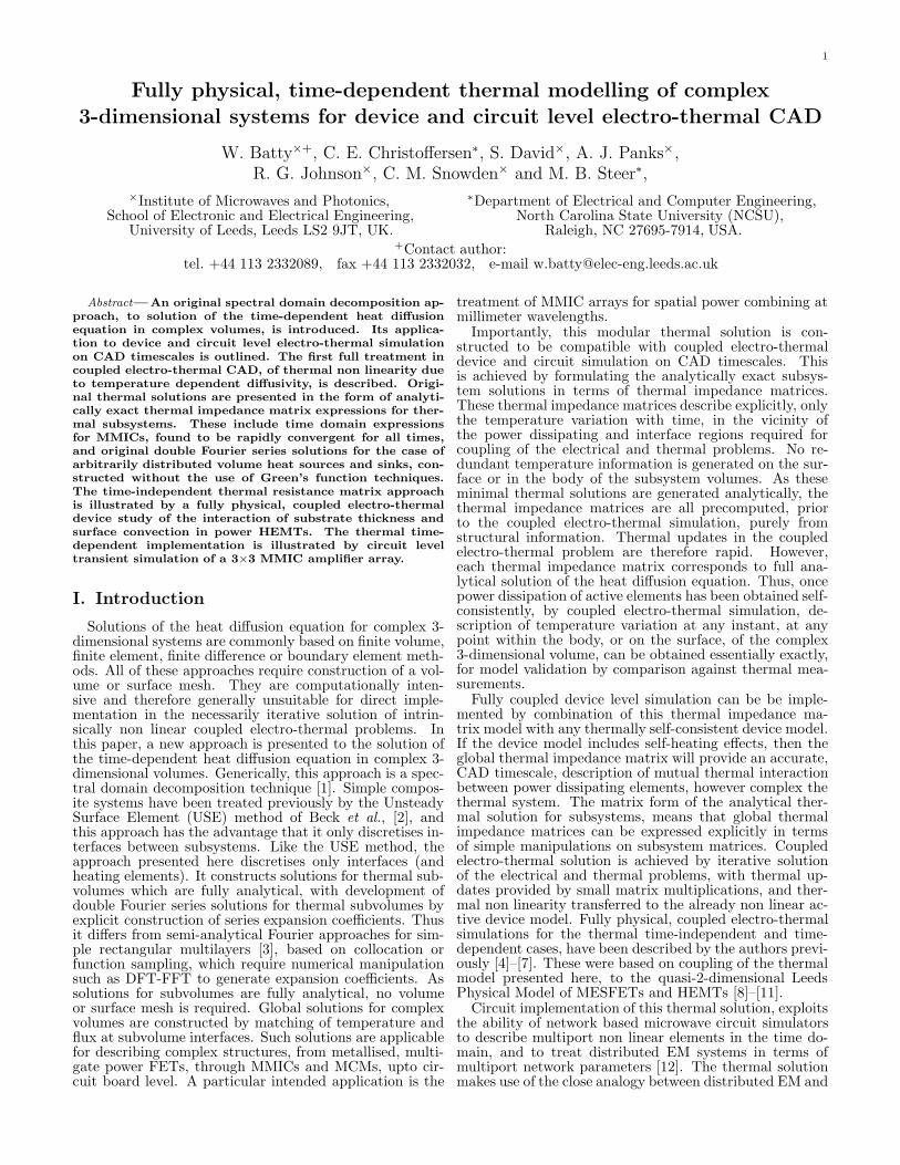
Fig. 1 shows plots of κ(T ) against T (solid line) and k(θ)against θ (dashed line), both normalised to their values atT = TS , assumed equal to 300 K. ρC has been assumedindependent of θ, which is a good approximation for semi-conductors. It is apparent that the Kirchhoff transforma-tion does not remove the temperature sensitivity of thematerial parameters for the time-dependent case.
Defining a new time variable, τ , by [22]
kSτ =∫ t
0
k(θ)dt, (4)
the time-dependent heat diffusion equation becomes fi-nally,
∇2θ − 1kS
∂θ
∂τ= − g
κS. (5)
The fully linearised equation, Eq. (5), can now be solvedexactly. To illustrate the significance of the time variabletransformation, Eq. (4), for electro-thermal response, ananalytical thermal impedance matrix is constructed to de-scribe the response to step power input of 0.4 W, over acentral square 0.1L× 0.1L, at the surface of a cubic GaAs
3
300 350 400 450 500Temperature (K)
0.0
0.2
0.4
0.6
0.8
1.0
Con
duct
ivity
, Diff
usiv
ity (
norm
alis
ed)
Fig. 1. Calculated temperature dependence of thermal conductivity,κ(T ), (solid line), and diffusivity, k(θ), (dashed line), in termsof physical temperature, T , and transformed temperature, θ, re-spectively. Kirchhoff transformation temperature, TS , is takento be 300 K.
die, side L = 400 µm. Such a configuration is illustrativeof, for example, a multi-finger power FET.
Eq. (4), for the integral transformation implies
dt
dτ=
kS
k (θ(τ))with t = 0 for τ = 0, (6)
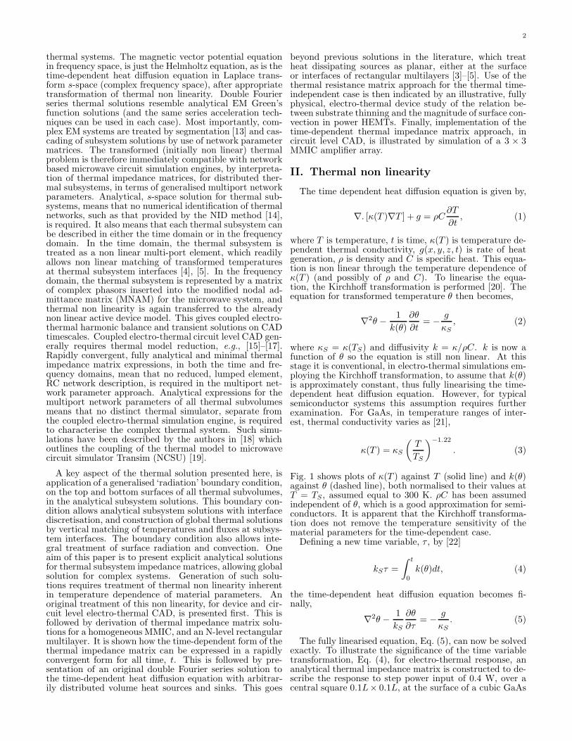
so as k (θ(τ)) is known from the analytical thermalimpedance matrix solution, Eq. (6) implies that physicaltime, t, can be obtained in terms of transformed time, τ ,by simple 1-dimensional numerical integration. Hence θ(t)is immediately recovered. Then performing the inverse ofthe Kirchhoff transformation, which is easily achieved an-alytically [5], physical active device temperatures are fi-nally obtained as a function of physical time, T (t). Fig.2, shows curves for the full, physical solution, T (t), afterboth inverse Kirchhoff and time variable transformations(solid line); the partially transformed solution, T (τ), afterinverse Kirchhoff transformation, but assuming constantdiffusivity, k(θ) = kS (dotted line); and transformed solu-tion θ(τ) neglecting both the inverse Kirchhoff and timevariable transformations, i.e., assuming the thermal prob-lem for the GaAs die is effectively fully linear (dashed line).
It is apparent that total neglect of thermal non linear-ity leads to a ∼30 K underestimate (dashed line) of thesteady-state temperature rise of ∼140 K (solid line). In-cluding the inverse Kirchhoff transformation, but neglect-ing the inverse time variable transformation (dotted line)is seen to overestimate the temperature rise by ∼4 % atany given instant, or equivalently, to underestimate the risetime required to reach a given temperature by as much as∼35 %.
Fig. 2 also shows a fourth curve (dot-dashed line),illustrating the sometimes used approximation of effec-tively linearising the time-dependent heat diffusion equa-tion about a typical operating point, without employingeither the Kirchhoff or the time variable transformation.This curve is obtained by assuming a constant diffusivity,kS , but with constant conductivity, κS , adjusted to re-flect the reduced value at elevated temperatures. ChoosingκS = 36.0 W/m.K corresponding to a temperature of 366.8K, instead of κS = 46.0 W/m.K corresponding to a tem-perature of 300 K, gives a calculated steady-state response
0 1 2 3 4 5log10(Time) (us)
325
345
365
385
405
425
445
Tem
pera
ture
(K
)
Fig. 2. Temperature rise with time (log10(t) µs), for a 0.1L× 0.1Lsquare heating element, at the top surface of a cubic die, sideL = 400 µm. Step-input power dissipation is 0.4 W. The resultsare calculated using an exact thermal impedance matrix solutionof the time-dependent heat diffusion equation. (i) solid line, T (t)(ii) dotted line, T (τ) (iii) dashed line, θ(τ) (iv) dot-dashed line,linearisation about a typical operating point.
accurate to within 0.5 K. However, it is apparent that theerror in this approximation is greater than that obtained byinvoking the Kirchhoff transformation, but neglecting thetime variable transformation (dotted line). Also, whereasT (t) (solid line), T (τ) (dotted line) and θ(τ) (dashed line),all tend to the same values at small times and temperaturerises, the fourth curve (dot-dashed line) shows a systematicoverestimate of temperature for all times compared to thefull numerical result (solid line). The error in the fourthapproach corresponds to ∼6 % overestimate of tempera-ture rise, or underestimate of rise time by as much as ∼60%. In addition, simply guessing a suitable operating pointfor linearisation is highly subjective, and for the case oftransient thermal variation of large amplitude, easily leadsto errors of ±5 K in the calculated steady-state operatingtemperatures.
Full linearisation of the time-dependent heat diffusionequation should therefore be implemented to obtain suffi-cient accuracy.
III. Analytical solutions
Having described the exact (not small signal) transfor-mation of the non linear time-dependent heat diffusionequation, to produce a fully linear problem, analytical so-lution of the linear problem in terms of thermal impedancematrices is now described.
A. The homogeneous MMIC
An analytical solution to the linearised heat diffusionequation, Eq. (5), is constructed for the case of a homo-geneous MMIC, 0 < x < L, 0 < y < W , 0 < z < D,with active device elements i = 1, ..., M described by sur-face elementary areas, Di. Adiabatic boundary conditionsare assumed on the side faces and a generalised ‘radia-tion’ boundary condition is imposed on the top and bottomfaces, z = 0, D. This can be written,
α0,DκS∂θ
∂z+H0,D (θ − θ0,D(x, y, t))+p0,D(x, y, t) = 0. (7)
4
Non linear boundary conditions can be treated in thelimit of a sequence of such fully linear problems [4], [23].Here, imposed flux densities p0,D(x, y, t) are time depen-dent. Coefficients H0,D describe surfaces fluxes due toradiation and convection. The α0,D equal zero for im-posed temperature boundary conditions and unity for im-posed flux boundary conditions. The respective ambienttemperatures (α0,D 6= 0), or heatsink mount tempera-tures (α0,D = 0), are also dependent on time, θ0,D(x, y, t).The generality of this boundary condition allows verticalmatching of thermal subsystems, by interface discretisa-tion and thermal impedance matrix manipulation, as wellas integral treatment of surface fluxes.
To solve this problem, the Laplace transform is con-structed giving,
∇2θ − 1kS
[sθ − θ(t = 0)
]= 0, (8)
assuming no volume sources or sinks, and describing sur-face fluxes by imposed boundary conditions, Eq. (7).
For the case of a uniform initial temperature distributionequal to uniform and time independent ambient tempera-ture, the substitution
Θ = sθ − θ(t = 0) (9)
is made, giving∇2Θ− s
kSΘ = 0. (10)
By separation of variables, the general solution for Θ is ofthe form,
Θ(s) =∑mn
cosλmx cos µny
× (Cmn cosh γmnz + Smn sinh γmnz)(11)
where m, n = 0, 1, 2, ..., and
λm =mπ
L, µn =
nπ
W, γ2
mn = λ2m + µ2
n +s
kS. (12)
Such fully analytical double Fourier series solutions inLaplace transform s-space have been described previously[24]. They are to be distinguished from semi-analyticalFourier solutions in frequency space, which are based oncollocation or function sampling, and require numericalmanipulation such as DFT-FFT to obtain expansion co-efficients [3].
With the transformation of variable, Eq. (9), the adia-batic side wall boundary conditions retain the same formand the radiation boundary condition on the top and bot-tom surfaces, z = 0, D, becomes
α0,DκS∂Θ∂z
+ H0,DΘ + sp0,D(x, y; s) = 0. (13)
Within this framework, the time-dependent problem re-sembles very closely the time-independent problem [4], [5],thus explicit forms for the expansion coefficients are ob-tained from,
H0Cmn = −γmnSmnα0κS −∫L
0
∫W
0cos(λmx) cos(µny)sp0(x,y;s)dxdy
LW4 (1+δm0)(1+δn0)
(14)
and
Cmn [αDκSγmn sinh(γmnD) + HD cosh(γmnD)]+ Smn [αDκSγmn cosh(γmnD) + HD sinh(γmnD)]
= −∫ L
0
∫ W
0cos(λmx) cos(µny)spD(x,y;s)dxdy
LW4 (1+δm0)(1+δn0)
. (15)
Here δmn is the Kronecker delta function and the standardresult,
L∫0
cosλmx cosλm′xdx =L
2δmm′ (1 + δm0δm′0) , (16)
has been used.As in the steady state case for the homogeneous MMIC
[4], [5], to illustrate a particular time-dependent form of thethermal impedance matrix, put α0 = 1, H0 = 0 (no radi-ation from the top surface, z = 0) and αD = 0, HD = 1,pD(x, y, t) = 0, θD(x, y, t) = θ(t = 0) (uniform tempera-ture on the bottom surface, z = D, corresponding to heatsink mounting at ambient temperature). Assume a surfacepower density of the form,
p0(x, y, t) =∑
i
Si(x, y)Pi(t), (17)
where Si(x, y) = 1 in active device elementary areas Di,and Si(x, y) = 0 otherwise, then
p0 =∑
i
Si(x, y)P i. (18)
The corresponding temperature distribution is given by
1sΘ(s) = −
∑mn
cosλmx cosµny ×
1κsLW
4(1 + δm0)(1 + δn0)
∑i
Iimn
1γmn
×
(sinh γmnz − tanh γmnD cosh γmnz)Pi, (19)
with area integrals Iimn defined by
Iimn =
∫∫Di
cos(mπx
L
)cos
(nπy
W
)dxdy. (20)
Constructing the surface temperatures averaged over ele-mentary areas Di as,
Θavi =
∫∫Di
Θ|z=0 dxdy∫∫Di
dxdy, (21)
immediately gives the defining equation of the thermalimpedance matrix approach,
θavi −θ(t = 0)
s=
∑j
RTHij (s)Pj , (22)
where,
RTHij (s) =1
κSLW
∑mn
4 tanh(γmnD)γmn(1 + δm0)(1 + δn0)
IimnIj
mn
Ii00
.
(23)
5
Extension to treat other realisations of the radiativeboundary condition, Eq. (7), is immediate. This allowsconstruction of solutions for large area substrates, with ra-diation and convection, and generation of series solutionsfor thermal subsystems with discretised interfaces, for ver-tical matching of thermal subvolume solutions in complex3-dimensional systems. The expression for RTHij (s), Eq.(23), can be written in alternative equivalent forms [24],and is readily extended to treat N-level multilayers [24].The temperature distribution of Eq. (19), and the corre-sponding thermal impedance matrix of Eq. (23), reduceto the respective steady-state forms [4], [5], in the limits/k → 0, giving for the thermal resistance matrix,
RTHij =
1κSLW
[DIj
00 +′∑
mn
4 tanh(ΓmnD)Γmn(1 + δm0)(1 + δn0)
IimnIj
mn
Ii00
](24)
where now, Γ2mn = λ2
m + µ2n, and the sum
∑′mn is over all
m, n = 0, 1, 2, ... excluding (m, n) = (0, 0).The solution of the heat diffusion equation just de-
scribed, provides analytical expressions for both the ther-mal impedance matrix and for the corresponding tempera-ture distribution throughout the body of the MMIC. Thismeans that once power dissipations, Pi, have been obtainedself-consistently, by employing the thermal impedance ma-trix in the coupled electro-thermal implementation, tem-perature can be obtained essentially exactly, if required, atany point within the body or on the surface of the MMIC.This is of value for model validation against measured ther-mal images.
These analytical expressions describe exactly the finitevolume of the die and the finite extent of transistor fingers,without making any approximations for infinite volume orfinite end effects. The elements of the matrices can besimply summed to give the total average temperature risedescribed by a single thermal resistance. These matrixexpressions represent an essentially exact description of 3-dimensional heat flow in the body of the die.
The series solutions can be partially summed in closedform using the Watson transformation [25], and partiallyaccelerated using the Poisson summation formula [26], togive even more rapidly evaluated expressions. These re-sults will be presented elsewhere.
Assuming the Pi to represent step inputs of magnitudePi, and combining tables of standard integrals, e.g., [2],with expressions for the inverse Laplace transform [27],gives the time-domain form of the thermal impedance ma-trix,
RTHij (t)
= 2κSLW Ij
00
{√ktπ + 2
∑∞l=1(−1)l
×[√
ktπ e−D2l2/(kt) −Dlerfc( Dl√
kt)]}
+ 1κSLW
∑′mn
4(1+δm0)(1+δn0)
IimnIj
mn
Ii00
1Γmn
×
erf(Γmn
√kt
)−∑∞
l=1(−1)l×
exp
{2DlΓmn+
ln[erfc
(Dl√kt
+ Γmn
√kt
)] }
− exp
{ −2DlΓmn+ln
[erfc
(Dl√kt− Γmn
√kt
)] }
(25)
This form of the time domain thermal impedance matrixis found to be rapidly convergent in the summation over lfor all t. It is an alternative to the explicit time constantform given in [18].
Even though analytical inversion is readily achieved, nu-merical inversion is algorithmically simple to implementand requires only evaluation of the Laplace transform anda corresponding weight function, at a small number of realor complex s-points [28]–[31],
L− {f(s)}t=τp=
∑µ
wµf(sµ), (26)
with wµ and sµ determined uniquely for a given τp. Typi-cally 5 or 6 s-points are adequate so this approach can becomputationally much cheaper than analytical inversion.
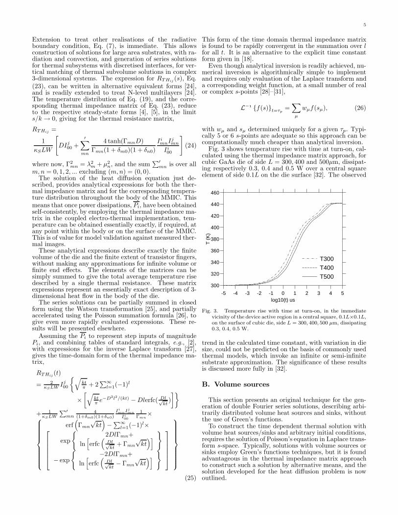
Fig. 3 shows temperature rise with time at turn-on, cal-culated using the thermal impedance matrix approach, forcubic GaAs die of side L = 300, 400 and 500µm, dissipat-ing respectively 0.3, 0.4 and 0.5 W over a central squareelement of side 0.1L on the die surface [32]. The observed
-5 -4 -3 -2 -1 0 1 2 3 4 5log10(t) us
300
320
340
360
380
400
420
440
460
T (
K)
T300
T400
T500
Fig. 3. Temperature rise with time at turn-on, in the immediatevicinity of the device active region in a central square, 0.1L×0.1L,on the surface of cubic die, side L = 300, 400, 500 µm, dissipating0.3, 0.4, 0.5 W.
trend in the calculated time constant, with variation in diesize, could not be predicted on the basis of commonly usedthermal models, which invoke an infinite or semi-infinitesubstrate approximation. The significance of these resultsis discussed more fully in [32].
B. Volume sources
This section presents an original technique for the gen-eration of double Fourier series solutions, describing arbi-trarily distributed volume heat sources and sinks, withoutthe use of Green’s functions.
To construct the time dependent thermal solution withvolume heat sources/sinks and arbitrary initial conditions,requires the solution of Poisson’s equation in Laplace trans-form s-space. Typically, solutions with volume sources orsinks employ Green’s functions techniques, but it is foundadvantageous in the thermal impedance matrix approachto construct such a solution by alternative means, and thesolution developed for the heat diffusion problem is nowoutlined.
6
Solving the time-dependent heat diffusion equation withvolume heat source in s-space,
∇2θ − s
kθ = −
[1κ
g(x, y, z) +θ(t = 0)
k
], (27)
and assuming a generalised double Fourier series solutionof the form,
θ(s) =∑mn
cosλmx cosµnyZmn(z), (28)
gives,d2Zmn
dz2− γ2
mnZmn = Gmn(z), (29)
where,
Gmn(z) =4
(1 + δm0)(1 + δn0)κLW×
∫ L
0
∫ W
0
cosλmx cos µny
[1κ
g(x, y, z) +θ(t = 0)
k
]dydx. (30)
To solve Eq. (29) write,
Zmn = eΓmnzzmn, (31)
and make the substitution,
ζmn =dzmn
dz, (32)
to reduce Eq. (29) to an equation of 1st-order in ζmn. Thislinear 1st-order equation can be solved by use of a simpleintegrating factor, giving the general solution,
Zmn = e−Γmnz
∫ z
0
e2Γmnz′∫ z′
0
e−Γmnz′′Gmn(z′′)dz′′dz′
+c1mn
2ΓmneΓmnz + c2mne−Γmnz , for (m, n) 6= (0, 0), (33)
(and c100 + c200 z for (m, n) = (0, 0).) This solution ofEq. (29) contains two arbitrary constants so is a generalsolution, valid for all boundary conditions. It is to be dis-tinguished from a Green’s function solution constructed fora δ-function source, with in-built boundary conditions.
These solution techniques are individually implicit intexts such as [33]. However, the authors believe thatthis double Fourier series method, for treatment of arbi-trary volume sources or sinks without use of Green’s func-tion techniques, represents an original approach to solu-tion of the time-independent and time-dependent heat dif-fusion equations. The double series solution, Eq. (28), isto be compared with much more computationally expen-sive triple series solutions obtained using Green’s functions.For the time-dependent case in s-space, this approach cangive both small-time and large-time series solutions, whichmay not be readily obtainable using Green’s functions.This approach is not discussed in texts such as [2], [34],[35].
This solution allows extension of the analytical ther-mal impedance matrix method to treat 3-dimensional vol-ume heat sources, rather than just the planar heat sources
that have been treated previously [3]–[5]. The ther-mal impedance matrix for power dissipating volumes, dis-tributed arbitrarily through the body of a MMIC, is givenby
RTHij (s) =1
κLW
∑mn
IimnIj
mn
Ii00
4(1 + δm0)(1 + δn0)
1γ2
mn
×
sinh γmnzi2−sinh γmnzi1γmn(zi2−zi1) ×
[cosh γmn(D−zi1)−cosh γmn(D−zi2)]cosh γmnD
+1− sinh γmn(zi2−zi1)γmn(zi2−zi1)
.
(34)
Here, zi1, zi2 are the z-coordinates of the planes boundingheat dissipating volume, i, in the z-direction, and the Ii
mnare the area integrals over the x − y cross-sections, Di,of heat dissipating volumes, i, Eq. (20). This expressionis to be compared with the thermal impedance matrix forpower dissipating surface areas, Eq. (23). Taking the limit,zi2 → zi1, gives the solution for a die with surface dissipat-ing areas distributed arbitrarily throughout its volume, ofvalue for instance in describing the buried channels belowthe semiconductor surface of a multi-gate power FET. Tak-ing the further limit, zi2, zi1 → 0, reproduces the solutionof Eq. (23).
This solution also makes possible treatment of the time-dependent problem for other than homogeneous initialconditions. It therefore allows construction of a time-stepping thermal impedance matrix formulation for tran-sient electro-thermal simulations, with repeated resettingof initial conditions. Details will be presented elsewhere.
C. Rectangular N-layer
The simple descriptions of the homogeneous MMIC, pre-sented above, are readily generalised to treat multi-layersystems by use of a transfer matrix, or two-port network,approach [36]. This is based on matching of Fourier com-ponents at interfaces, and corresponds to use of the doublecosine transform to convert the 3-dimensional partial dif-ferential equation, Eq. (5), into a 1-dimensional ordinarydifferential equation for the z-dependent double Fourierseries coefficients. Matching of linearised temperature andflux at the interfaces of a multi-layer structure can then beimposed by use of a 2 × 2 transfer matrix on the Fourierseries coefficients and their derivatives. Arbitrary N-levelstructures can be treated. Different thermal conductivi-ties can be assumed in each layer allowing treatment ofcomposites like Cu on AlN (both having temperature in-dependent thermal conductivities) and MMIC’s with con-ductivities varying from layer to layer due to differences indoping levels (all layers having the same functional formfor the temperature dependence of the conductivity).
The corresponding form for the thermal impedance ma-trix is,
RTHij (s) =∑mn
cosλmxj cosµnyj (Amn/Bmn)×
−4
κ1LW (1 + δm0)(1 + δn0)γ(1)mn
Iimn, (35)
where,(AmnBmn
)= M (1)M (2)...M (N−1)
(1
−cothγ(N)mn DN
),
(36)
7
with,
γ(r)mn =
(λ2
m + µ2n +
s
kr
)1/2
, (37)
and the layers have thickness, Dr, thermal conductivity,κr, and diffusivity kr, r = 1, ..., N , respectively. The M (r)
are analytically obtained 2 × 2 matrices, determined en-tirely by κr, κr+1, γ
(r)mn, γ
(r+1)mn and Dr.
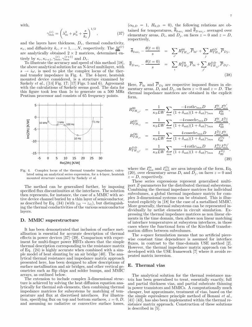
To illustrate the accuracy and speed of this method [18],the above analytical solution for an N-level multilayer, withs → iω, is used to plot the complex locus of the ther-mal transfer impedance in Fig. 4. The 4-layer, heatsinkmounted device considered, is a structure examined bySzekely et al., ([14] Fig. 17; [17] Figs. 5 and 6). Agreementwith the calculations of Szekely seems good. The data forthis figure took less than 1s to generate on a 500 MHzPentium processor and consists of 65 frequency points.
-5 0 5 10 15 20 25 30
Re(Zth) [K/W]
-15
-10
-5
0
5
Im(Z
th)
[K/W
]
1 Hz
10 Hz
100 Hz1 kHz10 kHz
Fig. 4. Complex locus of the thermal transfer impedance, calcu-lated using an analytical series expression, for a 4-layer, heatsinkmounted structure examined by Szekely et al.
The method can be generalised further, by imposingspecified flux discontinuities at the interfaces. The solutionthen represents, for instance, the case of a MMIC with ac-tive device channel buried by a thin layer of semiconductor,as described by Eq. (34) (with zi2 → zi1), but distinguish-ing the thermal conductivities of the various semiconductorlayers.
D. MMIC superstructure
It has been demonstrated that inclusion of surface met-allisation is essential for accurate description of thermaleffects in power devices [37]–[39]. Comparison with exper-iment for multi-finger power HBTs shows that the simplethermal description corresponding to the resistance matrixof Eq. (24) is highly accurate when combined with a sim-ple model of heat shunting by an air bridge [40]. The ana-lytical thermal resistance and impedance matrix approachpresented here, has been designed to allow descriptions ofsurface metallisation and air bridges, and other vertical ge-ometries such as flip chips and solder bumps, and MMICarrays, as outlined below.
The extension to include complex 3-dimensional struc-ture is achieved by solving the heat diffusion equation ana-lytically for thermal sub elements, then combining thermalimpedance matrices for subsystems by matching of tem-perature and flux at discretised interfaces. For illustra-tion, specifying flux on top and bottom surfaces, z = 0, D,and assuming no radiative or convective surface losses,
(α0,D = 1, H0,D = 0), the following relations are ob-tained for temperatures, θ0 avi and θD avj , averaged overelementary areas, Di, and Dj, on faces z = 0 and z = D,respectively,
θ0 avi −θ(t = 0)
s=
∑i′
R00THii′ P 0i′ +
∑j
R0DTHij
PDj ,
θD avj −θ(t = 0)
s=
∑i
RD0THji
P 0i +∑j′
RDDTHjj′ PDj′ .
(38)
Here, P 0i and PDj are respective imposed fluxes in ele-mentary areas, Di and Dj , on faces z = 0 and z = D. Thethermal impedance matrices are obtained in the explicitform,
R00THii′ =
1κSLW
∑mn
−4 cothγmnD
(1 + δm0)(1 + δn0)γmn
I0imnI0i′
mn
I0i00
,
R0DTHij
=1
κSLW
∑mn
−4 cosechγmnD
(1 + δm0)(1 + δn0)γmn
I0imnIDj
mn
I0i00
,
RD0THji
=1
κSLW
∑mn
4 cosechγmnD
(1 + δm0)(1 + δn0)γmn
IDjmnI0i
mn
IDj00
,
RDDTHjj′ =
1κSLW
∑mn
−4 cothγmnD
(1 + δm0)(1 + δn0)γmn
IDjmnIDj′
mn
IDj00
,
(39)
where the I0imn and IDj
mn are area integrals of the form, Eq.(20), over elementary areas Di and Dj, on faces z = 0 andz = D, respectively.
These series expressions represent generalised multi-port Z-parameters for the distributed thermal subsystems.Combining the thermal impedance matrices for individualsubvolumes, a global thermal impedance matrix for com-plex 3-dimensional systems can be obtained. This is illus-trated explicitly in [18] for the case of a metallised MMIC.More generally, thermal subsystems can be represented in-dividually by netlist elements in circuit simulation. Ex-pressing the thermal impedance matrices as non linear ele-ments in the time domain, then allows non linear matchingof interface temperatures at subsystem interfaces, in thosecases where the functional form of the Kirchhoff transfor-mation differs between subvolumes.
The s-space formulation means that no artificial piece-wise constant time dependence is assumed for interfacefluxes, in contrast to the time-domain USE method [2].However, the thermal impedance matrix approach can bedeveloped with the USE framework [7] where it avoids re-peated matrix inversion.
E. Thermal vias
The analytical solution for the thermal resistance ma-trix has been generalised to treat, essentially exactly, fulland partial thickness vias, and partial substrate thinningin power transistors and MMICs. A computationally muchcheaper, but approximate, treatment of vias, based on thethe simple equivalence principle method of Bonani et al.,[41]–[43], has also been implemented within the thermal re-sistance matrix approach. Construction of these solutionsis described in [5].
8
IV. Coupled electro-thermal approach
The thermal impedance matrix in s-space can be useddirectly in coupled electro-thermal harmonic balance sim-ulations. In this case the matrix of frequency dependentcomplex phasors corresponds to the network parameters ofthe distributed multi-port thermal network. It is inserteddirectly into the MNAM for the microwave system and sodoes not increase the number of non linear equations de-scribing the coupled solution.
In the coupled electro-thermal transient problem,Laplace transformed active power dissipations, P j(s),are not known explicitly and must be obtained by self-consistent solution. To combine the electrical and ther-mal descriptions, the corresponding Pj(t) must thereforebe discretised in time. Dividing the time interval of in-terest into equal subintervals of length δt, with the Pj(t)taking the piecewise constant form (for illustration)
Pj(t) = P(n)j for (n− 1)δt < t ≤ nδt, n = 1, ..., N (40)
then gives
P j(s) =∑
n
1s(1− e−sδt)e−(n−1)sδtP
(n)j . (41)
Inverting the impedance matrix equation, Eq (22), thetemperature rise of active element i at time t = mδt,∆θ
(m)i , is obtained as a function of the P
(n)j . Writing
∆θ(m)i = ∆θ
(m)i (P (m)
i ) from the electrical model then gives
∆θ(m)i (P (m)
i )=
∑j L−
{RTHij (s)P j(s)
}t = mδt
=∑
j
∑n u(m− n + 1)
×L−{RTHij (s)
s (− e−sδt)
}t =(m−n+)δt
P(n)j
=∑
j
∑n u(m− n + 1)[
RTHij ((m− n + 1)δt)−RTHij ((m− n + 2)δt)]P
(n)j
(42)where u is the unit step function,
u(x) ={
0, x < 01, x ≥ 0 , (43)
and the P(n)j are fluxes at timesteps, n. This corresponds
to N systems of equations in M unknowns, where N isthe number of discretised time points in the time inter-val under consideration, and M is the number of heatingelements. The Laplace inversion, with piecewise constantpower dissipation, avoids any explicit convolution opera-tion.
The entire thermal description is therefore obtainedby precomputation of RTHij (t) at timesteps, t = mδt,m = 0, ..., N . These precomputed values can be storedfor repeated re-use in different electro-thermal simulations.For reduction of precomputation time, the RTHij (t) can begenerated at intervals, and interior points obtained accu-rately by interpolation. This is a time-domain approachequivalent to representation of a frequency space transferfunction by a polynomial fit.
Extension to linear, quadratic or higher order interpola-tion of the active device power dissipations in each subin-terval, δt, is immediate, and for sufficiently short steplengths, low orders of interpolation should be required.
After self-consistent electro-thermal solution, and inver-sion of the Kirchhoff and time variable transformations,physical active device temperatures are finally obtained asa function of physical time, Ti(t), and electrical solutions,DC or RF, are determined.
V. Device Simulation
To illustrate the value of the analytical thermalimpedance matrix approach for coupled electro-thermalsimulations, the fully physical simulation of power FET’sis now described for the time-independent case. The ther-mal resistance matrix model is coupled to the Leeds Phys-ical Model (LPM). This is a quasi-2-dimensional model ofMESFET’s and HEMT’s [8]–[11]. It makes fully physicalprediction of device performance based solely on specifiedlayer compositions and doping levels and details of thedevice cross-section. It is thermally self-consistent, withdevice self-heating described by a temperature dependentmobility. The LPM requires no prior experimental devicecharacterisation.
For the coupled electro-thermal solution, transistor ac-tion described by the thermally self-consistent devicemodel gives the non linear relation,
∆θi = ∆θi(Pi). (44)
Here, the Kirchhoff transformation has been applied to ob-tain the function ∆θi(Pi) from the physical temperaturedependence of the model, so thermal non linearity has beenshifted from the thermal model to the already non linearactive device model. Combining the active device model,Eq. (44), with the global thermal description gives
∆θi(Pi) =∑
j
RTHij Pj (45)
which is a small, simple, non linear system to be solved self-consistently for the power densities, Pj . Having obtainedthe Pj at each bias point, from solution of the coupledelectro-thermal problems, Eq. (45), by a simple relaxationalgorithm, the full electrical solution is obtained and I-V curves are plotted. The temperature over the surfaceof the die, at a specified bias point, is obtained analyti-cally once individual finger power dissipations have beenobtained self-consistently.
Simulations are described of a 10-finger power HEMTprovided by Filtronic plc. [6]. In particular, these calcula-tions are used to ascertain the minimum physical descrip-tion compatible with accurate construction of the thermalresistance matrix, e.g. inclusion of surface metallisation,air bridges, vias or surface flux losses. To allow assessmentof the thermal impact on device performance of changesin parameters, the thermal resistance must be constructedfrom a physical model. This section describes applicationof the physical construction of the thermal resistance ma-trix for 10-finger Filtronic power HEMT FP4000, and itsuse in systematic study of the effects of substrate thinning,surface metallisation, vias and surface flux losses, on activechannel temperatures.
Flux losses from the surface of a die can, in principle,act to reduce the thermal resistance. Radiative losses areeasy to estimate and are orders of magnitude too small tohave any significant impact [4]. If convective losses are ofthe same order of magnitude as radiative losses, then thesetoo are insignificant. However, the magnitude of convec-tive losses from small areas with fine surface structure are
9
not easily estimated. Standard correlations from the liter-ature tend to be for large area substrates. In the absence ofa detailed model of fluid flow, significant convective lossesfrom the die surface could not be totally discounted, how-ever these effects have not been suggested in the literatureas significant at the scale of the FP4000 die.
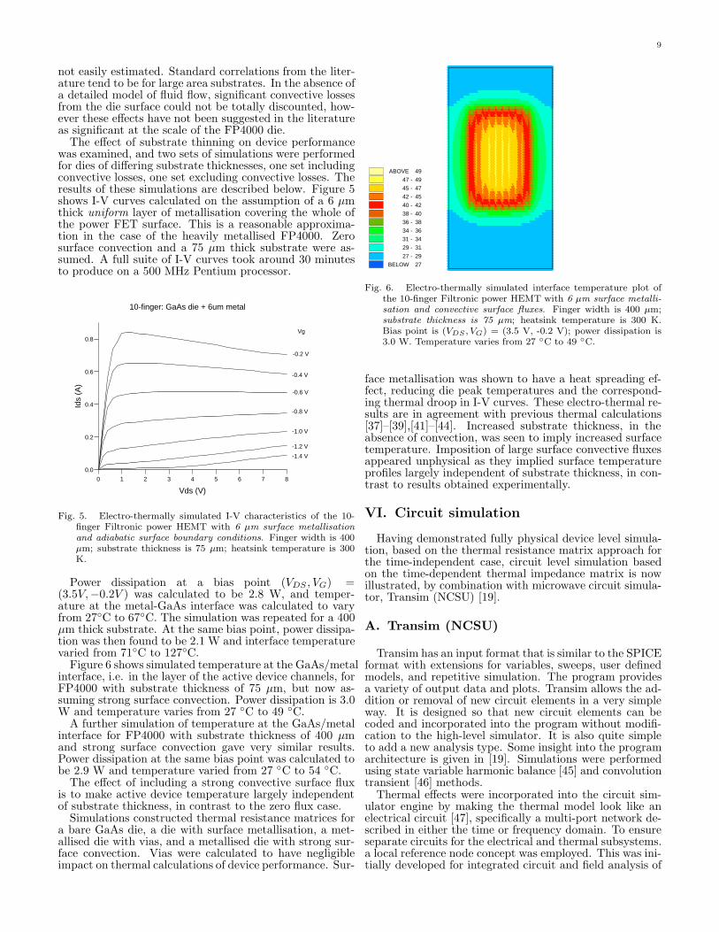
The effect of substrate thinning on device performancewas examined, and two sets of simulations were performedfor dies of differing substrate thicknesses, one set includingconvective losses, one set excluding convective losses. Theresults of these simulations are described below. Figure 5shows I-V curves calculated on the assumption of a 6 µmthick uniform layer of metallisation covering the whole ofthe power FET surface. This is a reasonable approxima-tion in the case of the heavily metallised FP4000. Zerosurface convection and a 75 µm thick substrate were as-sumed. A full suite of I-V curves took around 30 minutesto produce on a 500 MHz Pentium processor.
0 1 2 3 4 5 6 7 8
Vds (V)
0.0
0.2
0.4
0.6
0.8
Ids
(A)
Vg
-0.2 V
-0.4 V
-0.6 V
-0.8 V
-1.0 V
-1.2 V
-1.4 V
10-finger: GaAs die + 6um metal
Fig. 5. Electro-thermally simulated I-V characteristics of the 10-finger Filtronic power HEMT with 6 µm surface metallisationand adiabatic surface boundary conditions. Finger width is 400µm; substrate thickness is 75 µm; heatsink temperature is 300K.
Power dissipation at a bias point (VDS , VG) =(3.5V,−0.2V ) was calculated to be 2.8 W, and temper-ature at the metal-GaAs interface was calculated to varyfrom 27◦C to 67◦C. The simulation was repeated for a 400µm thick substrate. At the same bias point, power dissipa-tion was then found to be 2.1 W and interface temperaturevaried from 71◦C to 127◦C.
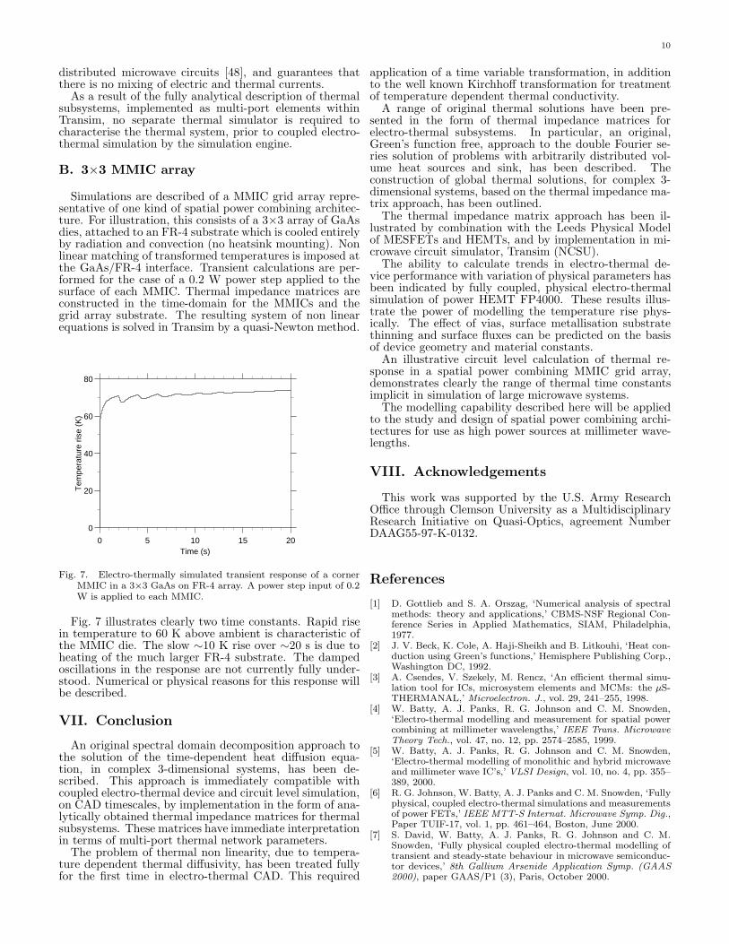
Figure 6 shows simulated temperature at the GaAs/metalinterface, i.e. in the layer of the active device channels, forFP4000 with substrate thickness of 75 µm, but now as-suming strong surface convection. Power dissipation is 3.0W and temperature varies from 27 ◦C to 49 ◦C.
A further simulation of temperature at the GaAs/metalinterface for FP4000 with substrate thickness of 400 µmand strong surface convection gave very similar results.Power dissipation at the same bias point was calculated tobe 2.9 W and temperature varied from 27 ◦C to 54 ◦C.
The effect of including a strong convective surface fluxis to make active device temperature largely independentof substrate thickness, in contrast to the zero flux case.
Simulations constructed thermal resistance matrices fora bare GaAs die, a die with surface metallisation, a met-allised die with vias, and a metallised die with strong sur-face convection. Vias were calculated to have negligibleimpact on thermal calculations of device performance. Sur-
BELOW 27
27 - 29
29 - 31
31 - 34
34 - 36
36 - 38
38 - 40
40 - 42
42 - 45
45 - 47
47 - 49
ABOVE 49
Fig. 6. Electro-thermally simulated interface temperature plot ofthe 10-finger Filtronic power HEMT with 6 µm surface metalli-sation and convective surface fluxes. Finger width is 400 µm;substrate thickness is 75 µm; heatsink temperature is 300 K.Bias point is (VDS , VG) = (3.5 V, -0.2 V); power dissipation is3.0 W. Temperature varies from 27 ◦C to 49 ◦C.
face metallisation was shown to have a heat spreading ef-fect, reducing die peak temperatures and the correspond-ing thermal droop in I-V curves. These electro-thermal re-sults are in agreement with previous thermal calculations[37]–[39],[41]–[44]. Increased substrate thickness, in theabsence of convection, was seen to imply increased surfacetemperature. Imposition of large surface convective fluxesappeared unphysical as they implied surface temperatureprofiles largely independent of substrate thickness, in con-trast to results obtained experimentally.
VI. Circuit simulation
Having demonstrated fully physical device level simula-tion, based on the thermal resistance matrix approach forthe time-independent case, circuit level simulation basedon the time-dependent thermal impedance matrix is nowillustrated, by combination with microwave circuit simula-tor, Transim (NCSU) [19].
A. Transim (NCSU)
Transim has an input format that is similar to the SPICEformat with extensions for variables, sweeps, user definedmodels, and repetitive simulation. The program providesa variety of output data and plots. Transim allows the ad-dition or removal of new circuit elements in a very simpleway. It is designed so that new circuit elements can becoded and incorporated into the program without modifi-cation to the high-level simulator. It is also quite simpleto add a new analysis type. Some insight into the programarchitecture is given in [19]. Simulations were performedusing state variable harmonic balance [45] and convolutiontransient [46] methods.
Thermal effects were incorporated into the circuit sim-ulator engine by making the thermal model look like anelectrical circuit [47], specifically a multi-port network de-scribed in either the time or frequency domain. To ensureseparate circuits for the electrical and thermal subsystems.a local reference node concept was employed. This was ini-tially developed for integrated circuit and field analysis of
10
distributed microwave circuits [48], and guarantees thatthere is no mixing of electric and thermal currents.
As a result of the fully analytical description of thermalsubsystems, implemented as multi-port elements withinTransim, no separate thermal simulator is required tocharacterise the thermal system, prior to coupled electro-thermal simulation by the simulation engine.
B. 3×3 MMIC array
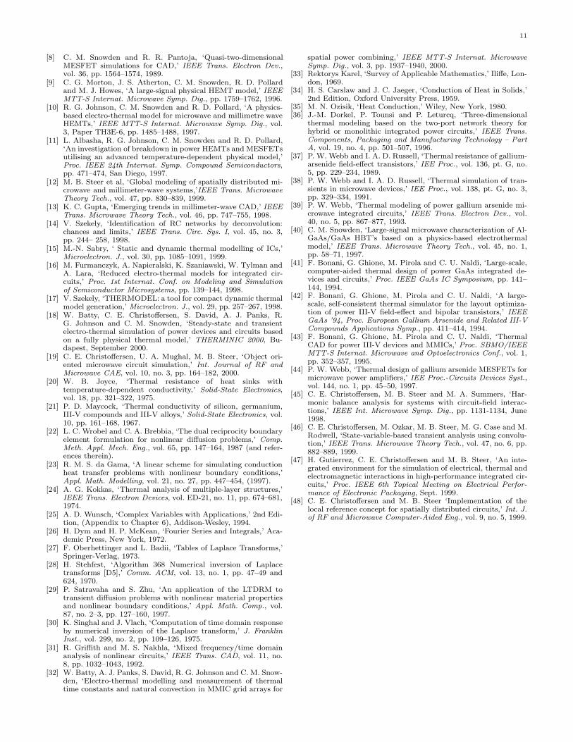
Simulations are described of a MMIC grid array repre-sentative of one kind of spatial power combining architec-ture. For illustration, this consists of a 3×3 array of GaAsdies, attached to an FR-4 substrate which is cooled entirelyby radiation and convection (no heatsink mounting). Nonlinear matching of transformed temperatures is imposed atthe GaAs/FR-4 interface. Transient calculations are per-formed for the case of a 0.2 W power step applied to thesurface of each MMIC. Thermal impedance matrices areconstructed in the time-domain for the MMICs and thegrid array substrate. The resulting system of non linearequations is solved in Transim by a quasi-Newton method.
0 5 10 15 20Time (s)
0
20
40
60
80
Tem
pera
ture
ris
e (K
)
Fig. 7. Electro-thermally simulated transient response of a cornerMMIC in a 3×3 GaAs on FR-4 array. A power step input of 0.2W is applied to each MMIC.
Fig. 7 illustrates clearly two time constants. Rapid risein temperature to 60 K above ambient is characteristic ofthe MMIC die. The slow ∼10 K rise over ∼20 s is due toheating of the much larger FR-4 substrate. The dampedoscillations in the response are not currently fully under-stood. Numerical or physical reasons for this response willbe described.
VII. Conclusion
An original spectral domain decomposition approach tothe solution of the time-dependent heat diffusion equa-tion, in complex 3-dimensional systems, has been de-scribed. This approach is immediately compatible withcoupled electro-thermal device and circuit level simulation,on CAD timescales, by implementation in the form of ana-lytically obtained thermal impedance matrices for thermalsubsystems. These matrices have immediate interpretationin terms of multi-port thermal network parameters.
The problem of thermal non linearity, due to tempera-ture dependent thermal diffusivity, has been treated fullyfor the first time in electro-thermal CAD. This required
application of a time variable transformation, in additionto the well known Kirchhoff transformation for treatmentof temperature dependent thermal conductivity.
A range of original thermal solutions have been pre-sented in the form of thermal impedance matrices forelectro-thermal subsystems. In particular, an original,Green’s function free, approach to the double Fourier se-ries solution of problems with arbitrarily distributed vol-ume heat sources and sink, has been described. Theconstruction of global thermal solutions, for complex 3-dimensional systems, based on the thermal impedance ma-trix approach, has been outlined.
The thermal impedance matrix approach has been il-lustrated by combination with the Leeds Physical Modelof MESFETs and HEMTs, and by implementation in mi-crowave circuit simulator, Transim (NCSU).
The ability to calculate trends in electro-thermal de-vice performance with variation of physical parameters hasbeen indicated by fully coupled, physical electro-thermalsimulation of power HEMT FP4000. These results illus-trate the power of modelling the temperature rise phys-ically. The effect of vias, surface metallisation substratethinning and surface fluxes can be predicted on the basisof device geometry and material constants.
An illustrative circuit level calculation of thermal re-sponse in a spatial power combining MMIC grid array,demonstrates clearly the range of thermal time constantsimplicit in simulation of large microwave systems.
The modelling capability described here will be appliedto the study and design of spatial power combining archi-tectures for use as high power sources at millimeter wave-lengths.
VIII. Acknowledgements
This work was supported by the U.S. Army ResearchOffice through Clemson University as a MultidisciplinaryResearch Initiative on Quasi-Optics, agreement NumberDAAG55-97-K-0132.
References
[1] D. Gottlieb and S. A. Orszag, ‘Numerical analysis of spectralmethods: theory and applications,’ CBMS-NSF Regional Con-ference Series in Applied Mathematics, SIAM, Philadelphia,1977.
[2] J. V. Beck, K. Cole, A. Haji-Sheikh and B. Litkouhi, ‘Heat con-duction using Green’s functions,’ Hemisphere Publishing Corp.,Washington DC, 1992.
[3] A. Csendes, V. Szekely, M. Rencz, ‘An efficient thermal simu-lation tool for ICs, microsystem elements and MCMs: the µS-THERMANAL,’ Microelectron. J., vol. 29, 241–255, 1998.
[4] W. Batty, A. J. Panks, R. G. Johnson and C. M. Snowden,‘Electro-thermal modelling and measurement for spatial powercombining at millimeter wavelengths,’ IEEE Trans. MicrowaveTheory Tech., vol. 47, no. 12, pp. 2574–2585, 1999.
[5] W. Batty, A. J. Panks, R. G. Johnson and C. M. Snowden,‘Electro-thermal modelling of monolithic and hybrid microwaveand millimeter wave IC’s,’ VLSI Design, vol. 10, no. 4, pp. 355–389, 2000.
[6] R. G. Johnson, W. Batty, A. J. Panks and C. M. Snowden, ‘Fullyphysical, coupled electro-thermal simulations and measurementsof power FETs,’ IEEE MTT-S Internat. Microwave Symp. Dig.,Paper TUIF-17, vol. 1, pp. 461–464, Boston, June 2000.
[7] S. David, W. Batty, A. J. Panks, R. G. Johnson and C. M.Snowden, ‘Fully physical coupled electro-thermal modelling oftransient and steady-state behaviour in microwave semiconduc-tor devices,’ 8th Gallium Arsenide Application Symp. (GAAS2000), paper GAAS/P1 (3), Paris, October 2000.
11
[8] C. M. Snowden and R. R. Pantoja, ‘Quasi-two-dimensionalMESFET simulations for CAD,’ IEEE Trans. Electron Dev.,vol. 36, pp. 1564–1574, 1989.
[9] C. G. Morton, J. S. Atherton, C. M. Snowden, R. D. Pollardand M. J. Howes, ‘A large-signal physical HEMT model,’ IEEEMTT-S Internat. Microwave Symp. Dig., pp. 1759–1762, 1996.
[10] R. G. Johnson, C. M. Snowden and R. D. Pollard, ‘A physics-based electro-thermal model for microwave and millimetre waveHEMTs,’ IEEE MTT-S Internat. Microwave Symp. Dig., vol.3, Paper TH3E-6, pp. 1485–1488, 1997.
[11] L. Albasha, R. G. Johnson, C. M. Snowden and R. D. Pollard,‘An investigation of breakdown in power HEMTs and MESFETsutilising an advanced temperature-dependent physical model,’Proc. IEEE 24th Internat. Symp. Compound Semiconductors,pp. 471–474, San Diego, 1997.
[12] M. B. Steer et al, ‘Global modeling of spatially distributed mi-crowave and millimeter-wave systems,’IEEE Trans. MicrowaveTheory Tech., vol. 47, pp. 830–839, 1999.
[13] K. C. Gupta, ‘Emerging trends in millimeter-wave CAD,’ IEEETrans. Microwave Theory Tech., vol. 46, pp. 747–755, 1998.
[14] V. Szekely, ‘Identification of RC networks by deconvolution:chances and limits,’ IEEE Trans. Circ. Sys. I, vol. 45, no. 3,pp. 244– 258, 1998.
[15] M.-N. Sabry, ‘ Static and dynamic thermal modelling of ICs,’Microelectron. J., vol. 30, pp. 1085–1091, 1999.
[16] M. Furmanczyk, A. Napieralski, K. Szaniawski, W. Tylman andA. Lara, ‘Reduced electro-thermal models for integrated cir-cuits,’ Proc. 1st Internat. Conf. on Modeling and Simulationof Semiconductor Microsystems, pp. 139–144, 1998.
[17] V. Szekely, ‘THERMODEL: a tool for compact dynamic thermalmodel generation,’ Microelectron. J., vol. 29, pp. 257–267, 1998.
[18] W. Batty, C. E. Christoffersen, S. David, A. J. Panks, R.G. Johnson and C. M. Snowden, ‘Steady-state and transientelectro-thermal simulation of power devices and circuits basedon a fully physical thermal model,’ THERMINIC 2000, Bu-dapest, September 2000.
[19] C. E. Christoffersen, U. A. Mughal, M. B. Steer, ‘Object ori-ented microwave circuit simulation,’ Int. Journal of RF andMicrowave CAE, vol. 10, no. 3, pp. 164–182, 2000.
[20] W. B. Joyce, ‘Thermal resistance of heat sinks withtemperature-dependent conductivity,’ Solid-State Electronics,vol. 18, pp. 321–322, 1975.
[21] P. D. Maycock, ‘Thermal conductivity of silicon, germanium,III-V compounds and III-V alloys,’ Solid-State Electronics, vol.10, pp. 161–168, 1967.
[22] L. C. Wrobel and C. A. Brebbia, ‘The dual reciprocity boundaryelement formulation for nonlinear diffusion problems,’ Comp.Meth. Appl. Mech. Eng., vol. 65, pp. 147–164, 1987 (and refer-ences therein).
[23] R. M. S. da Gama, ‘A linear scheme for simulating conductionheat transfer problems with nonlinear boundary conditions,’Appl. Math. Modelling, vol. 21, no. 27, pp. 447–454, (1997).
[24] A. G. Kokkas, ‘Thermal analysis of multiple-layer structures,’IEEE Trans. Electron Devices, vol. ED-21, no. 11, pp. 674–681,1974.
[25] A. D. Wunsch, ‘Complex Variables with Applications,’ 2nd Edi-tion, (Appendix to Chapter 6), Addison-Wesley, 1994.
[26] H. Dym and H. P. McKean, ‘Fourier Series and Integrals,’ Aca-demic Press, New York, 1972.
[27] F. Oberhettinger and L. Badii, ‘Tables of Laplace Transforms,’Springer-Verlag, 1973.
[28] H. Stehfest, ‘Algorithm 368 Numerical inversion of Laplacetransforms [D5],’ Comm. ACM, vol. 13, no. 1, pp. 47–49 and624, 1970.
[29] P. Satravaha and S. Zhu, ‘An application of the LTDRM totransient diffusion problems with nonlinear material propertiesand nonlinear boundary conditions,’ Appl. Math. Comp., vol.87, no. 2–3, pp. 127–160, 1997.
[30] K. Singhal and J. Vlach, ‘Computation of time domain responseby numerical inversion of the Laplace transform,’ J. FranklinInst., vol. 299, no. 2, pp. 109–126, 1975.
[31] R. Griffith and M. S. Nakhla, ‘Mixed frequency/time domainanalysis of nonlinear circuits,’ IEEE Trans. CAD, vol. 11, no.8, pp. 1032–1043, 1992.
[32] W. Batty, A. J. Panks, S. David, R. G. Johnson and C. M. Snow-den, ‘Electro-thermal modelling and measurement of thermaltime constants and natural convection in MMIC grid arrays for
spatial power combining,’ IEEE MTT-S Internat. MicrowaveSymp. Dig., vol. 3, pp. 1937–1940, 2000.
[33] Rektorys Karel, ‘Survey of Applicable Mathematics,’ Iliffe, Lon-don, 1969.
[34] H. S. Carslaw and J. C. Jaeger, ‘Conduction of Heat in Solids,’2nd Edition, Oxford University Press, 1959.
[35] M. N. Ozisik, ‘Heat Conduction,’ Wiley, New York, 1980.[36] J.-M. Dorkel, P. Tounsi and P. Leturcq, ‘Three-dimensional
thermal modeling based on the two-port network theory forhybrid or monolithic integrated power circuits,’ IEEE Trans.Components, Packaging and Manufacturing Technology – PartA, vol. 19, no. 4, pp. 501–507, 1996.
[37] P. W. Webb and I. A. D. Russell, ‘Thermal resistance of gallium-arsenide field-effect transistors,’ IEE Proc., vol. 136, pt. G, no.5, pp. 229–234, 1989.
[38] P. W. Webb and I. A. D. Russell, ‘Thermal simulation of tran-sients in microwave devices,’ IEE Proc., vol. 138, pt. G, no. 3,pp. 329–334, 1991.
[39] P. W. Webb, ‘Thermal modeling of power gallium arsenide mi-crowave integrated circuits,’ IEEE Trans. Electron Dev., vol.40, no. 5, pp. 867–877, 1993.
[40] C. M. Snowden, ‘Large-signal microwave characterization of Al-GaAs/GaAs HBT’s based on a physics-based electrothermalmodel,’ IEEE Trans. Microwave Theory Tech., vol. 45, no. 1,pp. 58–71, 1997.
[41] F. Bonani, G. Ghione, M. Pirola and C. U. Naldi, ‘Large-scale,computer-aided thermal design of power GaAs integrated de-vices and circuits,’ Proc. IEEE GaAs IC Symposium, pp. 141–144, 1994.
[42] F. Bonani, G. Ghione, M. Pirola and C. U. Naldi, ‘A large-scale, self-consistent thermal simulator for the layout optimiza-tion of power III-V field-effect and bipolar transistors,’ IEEEGaAs ’94, Proc. European Gallium Arsenide and Related III-VCompounds Applications Symp., pp. 411–414, 1994.
[43] F. Bonani, G. Ghione, M. Pirola and C. U. Naldi, ‘ThermalCAD for power III-V devices and MMICs,’ Proc. SBMO/IEEEMTT-S Internat. Microwave and Optoelectronics Conf., vol. 1,pp. 352–357, 1995.
[44] P. W. Webb, ‘Thermal design of gallium arsenide MESFETs formicrowave power amplifiers,’ IEE Proc.-Circuits Devices Syst.,vol. 144, no. 1, pp. 45–50, 1997.
[45] C. E. Christoffersen, M. B. Steer and M. A. Summers, ‘Har-monic balance analysis for systems with circuit-field interac-tions,’ IEEE Int. Microwave Symp. Dig., pp. 1131-1134, June1998.
[46] C. E. Christoffersen, M. Ozkar, M. B. Steer, M. G. Case and M.Rodwell, ‘State-variable-based transient analysis using convolu-tion,’ IEEE Trans. Microwave Theory Tech., vol. 47, no. 6, pp.882–889, 1999.
[47] H. Gutierrez, C. E. Christoffersen and M. B. Steer, ‘An inte-grated environment for the simulation of electrical, thermal andelectromagnetic interactions in high-performance integrated cir-cuits,’ Proc. IEEE 6th Topical Meeting on Electrical Perfor-mance of Electronic Packaging, Sept. 1999.
[48] C. E. Christoffersen and M. B. Steer ‘Implementation of thelocal reference concept for spatially distributed circuits,’ Int. J.of RF and Microwave Computer-Aided Eng., vol. 9, no. 5, 1999.