a framework for improved training of sigma-pi networks...

IEEE TRANSACTIONS ON NEURAL NETWORKS, VOL. 6, NO. 4, JULY 1995 893

A Framework for Improved Training of Sigma-Pi Networks Malcolm Heywood, Member, IEEE and Peter Noakes, Member, IEEE

Abstract-This paper proposes and demonstrates a framework for Sigma-Pi networks such that the combinatorial increase in product terms is avoided. This is achieved by only implementing a subset of the possible product terms (sub-net Sigma-Pi). Appli- cation of a dynamic weight pruning algorithm enables redundant weights to be removed and replaced during the learning process, hence permitting access to a larger weight space than employed at network initialization. More than one learning rate is applied to ensure that the inclusion of higher order descriptors does not result in over description of the training set (memorization). The application of such a framework is tested using a problem requiring significant generalization ability. Performance of the resulting sub-net Sigma-Pi network is compared to that returned by optimal multi-layer perceptrons and general Sigma-Pi solutions.

I. INTRODUCTION EEDFORWARD neural networks incorporating product F terms, such as the Sigma-Pi Network [I], are known to

provide inherently more powerful mapping abilities [2] than their first-order brethren (i.e., multi-layer perceptrons (MLP) networks). For example, the use of second-order product terms inherently solves the EX-OR [3], [4], and clump bit (a form of edge detector) [ 5 ] problems. More usefully, single layer networks incorporating third-order product terms alone have been shown to implement invariance in object classification systems [6], [7]. In spite of these benefits, the MLP network is much more widely applied in practical applications than the Sigma-Pi network.

The main reason for neglecting the Sigma-Pi network lies in a combinatorial increase in the number of product terms, hence weights, as the number of stimuli increases [2]. Present methods employing product terms rely on a priori knowledge about the problem to preselect the product terms used [7], [8]. This inherently limits the number of applications to which Sigma-Pi networks are applied, as in most neural network applications little knowledge exists about the solution to the problem in question.

The aim of this paper is to suggest and demonstrate a general framework to allow the implementation of Sigma-Pi networks, without preempting the product terms employed or incurring excessively large weight counts, while still exceeding the generalization ability of MLP systems. The framework is demonstrated by incrementally adding the components defin-

ing the framework and comparing the performance at each stage to a MLP network using the same neural architecture. The framework for training Sigma-Pi networks consists of three components:

1) It provides different learning rates for each product term order employed by the Sigma-Pi network.

2) It only implements a subset of the total number of product terms, so avoiding excessive weight counts.

3) It includes a dynamic weight pruning (DWP) algorithm capable of identifying and removing redundant weights during the learning process. Once removed, higher order (HO) terms, are replaced by HO terms not presently a member of the weight subset.

Details of the backpropagation (BP) learning rule applied to train Sigma-Pi networks are summarized in Section 11. The importance of the activation range selection is emphasized and individual learning rates for each order incorporated into the learning rule. The dynamic weight pruning algorithm is introduced in Section 111, which includes an overview to the function of each component defined by the above framework.

Sections IV-VI1 sequentially incorporate the proposed Sigma-Pi training framework, empirically demonstrating network ability at each stage. The evaluation problem and the performance of the standard MLP and Sigma-Pi systems are presented in Section IV. Section V introduces individual learning rates for each Sigma-Pi order and discusses the resulting gains in generalization ability. The proposed pruning framework is applied to the MLP and general Sigma-Pi networks in Section VI. This provides new, best-case generalization performance levels for each network. Section VI1 introduces the sub-net implementation for the Sigma-Pi topology, therefore making the network practical to implement in large network topologies. The section concludes by comparing the generalization ability for the three network topologies (pruned MLP, pruned Sigma-Pi, and sub- net Sigma-Pi). Finally Section VI11 summarizes the main conclusions and indicates the directions of our current and further research.

11. SIGMA-PI LEARNING RULE BY BACKPROPAGATION

Manuscript received July 17, 1993; revised March 10, 1994 and June 20, 1994. This work was supported by the United Kingdom Engineering and

The MLP network can be ‘Onsidered a Of the Sigma-Pi network [l], and therefore the BP algorithm forms

Physical Sciences Research Council. the basis for deriving the Sigma-Pi learning rule [9]-[ll]. The authors are with the Department of Electronic Systems Engineering,

Universitv of Essex. Wivenhoe Park. Colchester. Essex. CO4 3SO. UK. The significance Of the activation range On the processing .I E E E i o g Number 9409396. performed by product combinations is important. Two basic

1045-9227/95$04.00 0 1995 IEEE

894 IEEE TRANSACTIONS ON NEURAL NETWORKS, VOL. 6, NO. 4, JULY 1995

B. Backward Pass Relationships: Output Layer Error

Following evaluation of a square error objective function, the BP node error relationship for pattern p , is defined as [l]

p z - dnet,, ay,, &etpz ‘

It may be shown that the output layer error is expressed in

1st order routes

aEP (3) - 8EP -

product nodes

the same manner as that of the MLP network case. Thus

I I

Fig. 1. Second order (2, 2, 1) Sigma-Pi.

ranges exist, a polarized scheme (e.g., 0 to 1) or a nonpolarized scheme (e.g., 4~0.5). In the case of a Sigma-Pi network, a product term will effectively solve the EX-OR problem if a nonpolarized scheme is used; a function which traditional MLP networks have difficulty in implementing. Product terms in the case of a polarized scheme provide an “AND’ function; a function easily implemented at a MLP neuron. Furthermore, in the case of the MLP system a nonpolarized representation has been shown to have better convergence characteristics in terms of reliability and convergence time [12]. Therefore, the nonpolarized scheme is employed for both MLP and Sigma-Pi networks in this analysis.

where f’(y,i) = 0.25 - ygi for the nonpolarized configuration employed here.

C. Backward Pass Relationships: Hidden Layer Error

As in BP, the same relationship is employed for the hidden layer error as the output layer error estimation, (3). The partial derivative of a node output with respect to node activation, i, remains unchanged while the remaining partial derivative is expanded using the chain rule in the BP manner to evaluate S p e , the error fed back from node e in the layer following that indexed by i.

Now, from (2), the neural inputs in this following layer are expressed as

Hence A. Sigma-Pi Feedforward Relationship

where the only difference in the feedforward relationships is the inclusion of extra terms within the stimuli at the receiving

(2, 2, 1) network (second order interconnects emphasized for clarity), where the general feedforward relationship is given by

1

anet,, - The Sigma-Pi network is a generalization of the MLP,

neuron. Fig. 1 illustrates a simple Sigma-Pi structure for a

- -

‘ Q e z 3 Y P ~ f W3e23k YPJ Y P ~ + ’ ’ ‘

( 5 )

Finally, substituting ( 5 ) into (3) provides the required hidden layer error backpropagation rule. (See (6) shown at the bottom of the page.)

k 3

(1) - 0.5 y z = 1 + exp (-net,)

where D. Weight Updating

and w n i j is the weight of the nth order product for the i destination neuron, j and IC index the product between stimuli and 7 is the threshold applied to neuron i .

Of note is the -0.5 component in (I) which applies an output range shift (as opposed to the input shift applied by the neuron threshold), hence providing a nonpolarized output over the range & - 0.5 [12].

Weight updating using the generalized delta rule is simply the product of error at the destination node and stimuli passing through the weight. For Sigma-Pi networks, the partial differ- ential of node activation with respect to weight is evaluated separately for each order the network contains. Hence, the update rules for first to third order product terms are

(7) 1st order (MLP relationship). Ai;j = V I S,i ypj

2nd order weight change. A W 2 i j k = 772 6,i ypj y p k

3rd order weight change. A w 3 ; j k l = 773 6,i ypj Ypk ypl (8) (9)

through partial differentiation of (2).

HEYWOOD AND NOAKES: A FRAMEWORK FOR IMPROVED TRAINING OF SIGMA-PI NETWORKS

r - - - -

N-L r - - - - - -

STABILITY criteria satisfied ?

Yl w

weight of LITTLE SIGNIFICANCE to neuron ?

Yi count of DWP criteria satistied

in iteration > DWP count requirement ?

Y Add weight to DWP short list I

1

895

1 -

BP Components _ . . . . . I

ContinueBP ) \ - - - - / Pruning Components

Fig. 2. Dynamic weight pruning at BP update cycle.

N.B.: the 71, component represents the user selected learning rate. It is proposed in Section V that these are specific to the product term orders employed.

111. DYNAMIC WEIGHT PRUNING

Weight pruning algorithms typically require network convergence before pruning is applied [ 131-[ 151 or that a penalty term is included to apply a weight decay over the period of the training cycle (e.g., [16] and [17]). This means that the network is restricted to using these HO weights included at initialization. The problem addressed by the authors is that of selecting an appropriate set of HO terms during the training cycle [18]-[20]. To do this, the point at which weightsheurons are representative of their target state must be identified. Such a target state is defined local to the neuron and typically will change during the training cycle. This is the purpose of the stability measure introduced by the authors in the context of a simple amendment to the BP algorithm [20]. Once stability is achieved, the significance of weights local to the target neuron is estimated with respect to a local objective function defined by the authors as a weight significance test. The application of

these two tests forms the basis of our dynamic weight pruning process. Pruning following network convergence only requires a weight significance test (cf., as in the weight saliency measure employed by [14] and [15]), where the significance measure at this stage is applied with respect to the global objective function.

The Sigma-Pi learning algorithm employs three stages during training, each with a distinct aim.

1) Dynamic weight pruning: extraction of redundant weights with replacement of HO terms to permit the inclusion of alternative product terms (Fig. 2).

2) Sparse network extraction: extraction of a minimal network configuration. Network training is halted near convergence and pruning is performed using the weight significance measure alone (with respect to the global objective function).

3) BP adaptation alone: following sparse network extraction the network structure is defined. Training continues until the final error criteria is satisfied, typically using a larger momentum term (this corresponds to the "retraining" period following optimal brain damage (OBD) pruning [14]).


A. Stage I : Dynamic Weight Pruning

Two criteria must be satisfied before a weight can be removed during pruning while the network is undergoing training, Fig. 2. The first is a stability measure which is concerned with the amount of variation weights undergo; when changes in the network stimuli have minimal effect on the weights local to a given neuron, these weights are considered representative of their present target state, and hence quantifiable against the local objective function. The mathematical interpretation of this is in terms of the rate of change of the weight update parameter under the influence of the stimuli passing through the weight in question. For first order terms this is expressed as [20]

where, Q! is the momentum term [l] and from (7)

For second order weights, two stimuli pass through the weight giving rise to terms of the form

where, from (8)

AW2, jk = r/z.si(t).yj(t).yl,(t)+ “ . S i . ( t - l).Yj(t - l).yrc(t - 1).

Similar expressions are forthcoming for third and higher order terms.

The result of this stability measure is that weights of a given order, local to a specific neuron, will test positive or negative with respect to some user specified threshold (the stability threshold). Following satisfaction of the stability measure by a neuron, the weight significance of each weight with respect to the objective function is determined. During the dynamic pruning stage, objective functions for pruning tests are applied locally to the neuron; at sparse net extraction the global objective function is employed. Such a distinction has more importance when more rigorous significance measures are used than the purely magnitude based method employed here [21], [22]. The satisfaction of both the stability measure and the weight significance test, is defined by the authors as satisfying the DWP criteria.

Previously [20], the weight significance test comprised a simple weight magnitude comparison between the actual weight magnitude and a user specified threshold (zero weight (ZW) threshold) representing the lowest saliency judged to be significant. This assumes that the weights of largest magnitude have most significance at the corresponding neuron (i.e., a local objective function), which has been demonstrated not to be true in all cases [14], [15].’ An alternative is to employ a saliency measure used in a more rigorous static pruning technique (e.g., [14] and [15]). To demonstrate a general framework for training Sigma-Pi networks, however, applied

’ Such a condition is only true when no bias is applied to the network during training, which by definition is not the case in this instance.

ZW threshold

ZW threshold adapt ion path

min

max error min (x 1) (Xz)

Fig. 3. Application of adaptive zero weight threshold.

to nonbinary problems, our original weight-magnitude based approach is employed, where the ZW threshold is adjusted adaptively as a function of the network RMS error during the dynamic pruning stage (within this framework we have also applied the optimal brain surgeon weight saliency measure [211-[231).

An adaptive ZW threshold is applied to alleviate com- promises in selecting a specific ZW threshold, below which all weights with a lower saliency are removed. An adaptive ZW threshold means that when the stability threshold is first satisfied, only those weights of least importance are selected for pruning. This prevents too many weights being removed too early in network evolution, reducing the network’s ability to avoid local minima. As the RMS error reduces with network training, the saliency severity is relaxed to allow an increase in the degree of pruning applied. The adaptive ZW threshold is defined by Fig. 3 and (12)

(12)

where, m = (gz - gl)/(x2 - xl)’, the parabola steepness, y1, yp are max and min ZW threshold, respectively, and, xp, 2 1

are max and min RMS error, respectively. Finally, some simple management controls (defined in

Fig. 4) are included to 1) limit the number of weights removed at any one neural

update, and 2) provide a weight reintroduction path (prudent, given the

simplicity of the weight significance test used).

ZW threshold=m.((present RMS error) + 21)’ + y p

B. Stage 2: Sparse Network Extraction

The aim here is to extract the most succinct network possible before the final error criteria is satisfied. Therefore, dynamic pruning is applied until a point is reached close to the required minimum error which defines when the network has completed training.

At this point the weights are assumed to be stable and representative of their final states. Therefore, the stability measure is no longer necessary and pruning is applied using the weight significance parameter alone. This corresponds to pruning using a static pruning algorithm, where pruning continues until no more weights can be removed without exceeding the maximum ZW threshold (y1 in Fig. 3).

C. Stage 3: BP Training with Updated Learning Parameters

With the above pruning stages completed, a network structure has been defined, and the remaining weights can be “pushed” toward the located minima by continuing training

HEYWOOD AND NOAKES: A FRAMEWORK FOR IMPROVED TRAINING OF SIGMA-PI NETWORKS 897

from weight identitied ea PRESENTLY set to zem

4 Inc (DWP criteria Count)

I

I RemnveWeighl -. OHlnl s~tidks Decrement

(DWP Crileria count) -. Weicht Remnve Pcrkd ? 7---

DWP Criteria munt PI Zem ? XI

DWP CRITERIA COUNTS

Decrement Step Size :

No DWD CntenaPatterns No Patterns In Training Set

Increment Step Size : Unity

. .

Weight replacement

Weight re - introduction

_ . . . . .

Fig. 4. Secondary controls and weight re-introduction.

TABLE I TRAINING AND TEST SET OBJECT ORIENTATIONS

Data Set

Training Set

Test Set 15" intervals

Object Orientations used in Data Set

0.60, 120, 180,240, 300

15, 30,45,75,90, 105, 135, 150. 165, 195,210, 225, 255,270, 285, 315, 330. 345

127, 163,274,85, 19,29,261, 153,246,263,322.89,341,257, 123,291, 347,259.26, 199,297.229.86, 122. 340.48, 179, 213, 2. 137

nndomintervals

with an increased momentum term. This process is typically short in duration and is similar to the retraining stage required following the use of static pruning algorithms.

Iv . EVALUATION TASK AND NETWORK ARCHITECTURES

The main objective is to demonstrate a framework for training Sigma-Pi networks without incurring the combinatorial explosion in product terms. To allow direct comparisons between the proposed framework and standard Sigma-Pi algorithm [l], [lo], [ l l], however, network size has to be small enough to allow a general implementation of the Sigma-Pi network. Furthermore, it was desirable that a MLP network be capable of solving the problem. These requirements provide limits to the range of candidate problems and network size.

A. Evaluation Task and Network Topology Selection

Other research interests dictated that a rotational-invariant object classification task be employed, such as those discussed in [24]. For our benchmark problem, objects are described by loo0 to 1500 pixels (approximately 64 by 64 pixel space) and are allowed to move about a larger input space. To limit the number of inputs "seen" by the network, central moments are applied and normalization applied implementing translation and scale invariance [25]-[30]. A total of seven central moment terms are extracted, corresponding to second- and third-order terms and form the basis of the network stimuli (Fig. 5).

The object of the system is to correctly classify the images into one of six classes. The test for network generalization requires the correct classification of rotational variant objects,

Central Mument MLP I Sigma ~ PI nctrurh Binary Digitned Image Space I I Exiracuon

Fig. 5. Movement invariant object classifier.

where training is performed using a restricted set of samples. The network training set only contains six rotated versions of each object taken at 60-degree intervals and no scaled or translated versions of the objects. The test set is composed of 18 rotated versions of each object taken at intervening 15- degree increments with respect to the training set patterns, and a further 30 randomly selected rotated versions of each object (Table I). The objects employed correspond to the first six upper case characters of the English alphabet (pixel count and dimensions as above). This provides a good classification test due to the similarity between letters B, E , and F . Raw moment data is limited to a dynamic range of f0.95 by selecting the largest magnitude term for each moment order in the test set, and employing this as a scalar to ensure that the input range is not exceeded. Such a scheme although simple, relies on the data itself for variation in sign but, this does not present a problem due to the strictly bound nature of the data set.

B. Architecture Selection

Various MLP structures with weights initialized using 20 different initializations were trained using the standard BP learning rule (internal activation range of f0 .5 [12]) to as-

898 IEEE TRANSACTIONS ON NEURAL NETWORKS, VOL. 6, NO. 4. JUL.Y 1995

TABLE I1 MLP CLASSIFICATION ACCURACY USING STANDARD LEARNING RULE

Network Type % Correct Iterations to Leaning Rate Classifications Convergence

7, 3.6

7,s) 6 61 - 5 2 1677 - 1162 I 7,7,6 62 - 50 1543 - 859 1

7, 10, 6 47 - 33 1096 - 1020 1

7, 3, 3,6

7, 4, 4, 6 75 - 61 I510 - 1098 0.8

7, 7,6,6 73 - 68 498 - 395 1

no convergence attained within 3000 iterations.

no convergence attained within 3000 iterations.

certain the MLP structure most suitable for the classifier. The structures included three layer and four layer networks, where the learning rates used ranged from 0.1 to 1.0 in 0.1 increments. Table I1 summarizes the classification performance for each network using the test set from Table I, excluding the randomly selected angles. The percentage of correct classifications is shown over the 20 initializations, for the learning rate providing the best generalization ability.

From Table 11 it is evident that the (7, 4, 4, 6) network returns the best classification performance. The (7, 7, 6, 6) network generalization performance is similar to that of the (7, 4, 4, 6) network, but has a better convergence characteristic. The (7, 7, 6, 6) topology also provides a better basis for the pruning process while the (7, 4, 4, 6) is already of a highly constrained nature. Consequently, the (7, 7, 6, 6) network defines the architecture employed for both MLP and Sigma-Pi networks in this paper. This biases the results in favor of the MLP network, as the “extra” nonlinear mapping ability of the Sigma-Pi network should mean that fewer neurons are required by such networks. It is important to remember, however, that the nonlinearities implemented by product terms in real valued data sets are not the same as those implemented in the MLP network. The nonlinearities of MLP networks are developed through the application of the neuron nonlinearity and its repeated nesting. Without a nonlinear element, any MLP system can be expressed by a perceptron relationship. Given a general Sigma-Pi network with the same neural structure, however, the input-output mapping provides two mechanisms for nonlinearities; nested sigmoid functions and product combinations. Removing the nonlinear activation function does not negate the networks ability to perform nonlinear mappings, but does result in an input-output relationship defined by a polynomial expansion, where the maximum order is defined by the product of the number of layers employed and the maximum Sigma-Pi order (assuming the same maximum order per layer).

The effect of changing the number of neurons employed in a general second-order Sigma-Pi network was determined by repeating the classification task described above for a selection of second order Sigma-Pi structures. The Sigma- Pi network was trained using the same learning rate for each product term order [l], [lo], [ll], but as in the MLP case, the learning rate is allowed to range from 0.1 to 1.0 in 0.1 increments. The classification results are summarized in Table 111. Three characteristics are immediately apparent. First,

TABLE I11 STANDARD SECOND-ORDER SIGMA-PI NETWORK PERFORMANCE

Network Type 9’0 Correct Iterations to Learning Rate Classifications Convergence

1.3.6 SI - 3 0 540 - 320 0.60

7.5, 6 41 - 28 450 - 338 0.50

7,7.6 43 - 30 I I38 - 955 0.20

I , 10, 6 39 - 21 21.5 - 172 0.90

7. 3. 3.6 29 163 0.90

7.4.4.6 S6 - 40 318 - 187 0.80

7.7,6,6 5 1 - 3 7 153 - I12 I 00

the classification accuracy never approaches the level achieved by the standard MLP network. Second, although the Sigma-Pi network never reaches the generalization ability of the MLP, the performance generally peaks for a network using a lower neuron, hence weight count, than the peak MLP cases. Finally, the Sigma-Pi network is trained using fewer iterations than the MLP equivalent.

V. TRAINING GENERAL SIGMA-PI NETWORKS USING ORDER SPECIFIC LEARNING RATES

The experiments using a general Sigma-Pi network discussed in Section IV indicate a poor level of performance with respect to the MLP architecture irrespective of the neuron count. Two characteristics worth emphasizing with respect to the Sigma-Pi network solution at this point are that 1) a large number of weights are employed and 2) learning is completed quickly. This is the over learning characteristic often observed in MLP networks employing too many neurons. A general Sigma-Pi network will always have “too many” weights, so a method is required to regulate the number of higher order terms employed.

Within the BP framework, the rate of learning is controlled by the learning rate parameter which dictates the amount by which the present weight update influences the next weight state. Present implementations of Sigma-Pi networks employ the same learning rate across all the orders employed. As indicated in Section IV, the inclusion of product terms provides two mechanisms for nonlinearities within the network, where the descriptive power of product terms increases with increasing order. Consequently, the application of these nonlinearities can only be controlled adequately using differing learning rates and therefore, the authors propose that HO term learning rates should be significantly lower than those for the first order terms. This results in a bias to perform mappings using the lowest order terms wherever possible, with the aim of providing the most general description while avoiding over fitting of training data.

To test this hypothesis the learning rate for first-order terms was set to 1.0 (the previously identified optimum), and the second-order learning rate varied between 0.1 and 2.6 using 0.2 steps. For each learning rate combination, 20 network initializations were employed using the (7, 7, 6, 6 ) and (7, 4, 4, 6) architectures. Fig. 6 summarizes the minimum RMS error for both experiments where the full test set data, Table I,


n 2 4 , I X

n 2 2

0 1 2 ‘ x

n i , I , I I I I I I

( 1 2 0 4 0 6 0 8 I 1 2 1 4 I 6 1 8 2 0 2 2 2 4

L e a r n i n g Rate f o r 2nd Order Terms

Fig. 6. for second order learning rate.

(7, 7, 6, 6) and (7, 4, 4, 6) Sigma-Pi network minimum RMS error

I - (7 ,7 ,6 .6 ) net + ( 7 , 4 , 4 . 6 ) net 1

575 I * i

c *

0 2 0 .4 n e , 0.8 I 1 . 2 1 4 1 6 i n 2 0 2 2 2 4 Learning Rate for 2nd Order Terms

Fig. 7. gence for second order learning rate.

(7, 7, 6, 6) and (7, 4, 4, 6) Sigma-Pi network iterations to conver-

is employed for evaluating the trained networks. Training was stopped when a maximum error of 0.1 was returned across training set patterns. Clearly classification accuracy is far better when the first order learning rate is in excess of the second. Predictably, a lower second order learning rate results in more iterations before convergence (Fig. 7).

Optimum classification accuracy for the (7, 7, 6, 6) Sigma- Pi network is returned when the second-order learning rate is reduced to 0.07. This results in a peak classification accuracy 3% greater than that for the equivalent MLP case (Table 11). This also represents a 22% improvement over the best case classification accuracy returned by the single learning rate instance for the Sigma-Pi network (Table 111). CPU simulation time favors the MLP system, indicating the inherent computational overheads and much larger network size (127 weights verses 617 weights using a (7, 7, 6, 6) network) resulting from general Si-Pi networks (Table IV).

VI. DYNAMIC WEIGHT PRUNING IN GENERAL SIGMA-PI AND MLP NETWORKS

It is now necessary to determine whether weight pruning results in the general Sigma-Pi network performing better than that for the MLP. Furthermore, to speed the pruning algorithm, the effect of permitting weights to be set to zero before they

TABLE IV MLP AND MULTIPLE LEARNING RATE GENERAL SIGMA-PI

NETWORK PERFORMANCE FOR ROTATION INVARIANCE PROBLEM

Best Case’ Network Mean’ Topology

iterations CPU time rms error Classification MLP 523 135 s 0.15 75 %

Siema - Pi2 257 368 s 0.12 78 %

I 20 network initialisations employed

1 st order term learning rate : 1 .O; 2nd order term learning rate : 0.07

satisfied the DWP criteria across the entire training set was investigated using the (7, 7, 6, 6) structure identified above.

The weight pruning process of Section 111 was employed. Table V summarizes the learning and pruning algorithm parameters used. Performance was evaluated in terms of three different categories: Weight requirement following convergence, iterations to convergence and CPU simulation time, and network generalization ability. For the remainder of the paper, unless otherwise indicated, the term “Sigma-Pi” network implies the use of multiple learning rates. “General” Sigma-Pi indicates that all the higher order weights are included, while sub-net Sigma-Pi indicates that the number of higher order terms per neuron is limited.

A. Weight Requirement at Convergence

There is close similarity between the total number of weights employed for pruned MLP and pruned general Sigma-Pi networks. Pruning removed 83% to 87% of the weights initially employed for the general Sigma-Pi network, hence indicating significant redundancy. In the case of the MLP network between 18% and 39% of the weights initially employed were removed. Following convergence, it was found that most second-order weights were employed in the first hidden layer, with only a few present in the output layer (true across all network initializations).

B. Iterations to Convergence and CPU Simulation Time

Two distinct effects are demonstrated between MLP and Sigma-Pi implementations irrespective of the DWP criteria employed. The Sigma-Pi case always converged using far fewer iterations (53%-58%) than the MLP case. The MLP, however, always required less simulation time (63%-73% of that for the Sigma-Pi case). The latter characteristic will be due to 1) the computational overhead involved in performing double precision floating point multiplications and 2) an increase in pruning activity resulting in more calls to the random number generator routine.

C. Network Generalization Ability

The peak performance for each network is employed as a measure of the network generalization ability (20 network initializations are employed for each structure). Fig. 8 depicts the classification accuracy, for MLP and general Sigma-Pi implementation, with and without pruning applied. In terms of classification accuracy the MLP network provides a 79.5%

900 EEE TRANSACTIONS ON NEURAL NETWORKS, VOL. 6, NO. 4. JULY 1995

TABLE V PRUNING AND LEARNING ALGORITHM PARAMETERS

BP Parameters Dynamic Weight Pruning Parameters

Leaming Rate 1st order 1 Stability threshold (n - learning rate; x - order) (nJ2.S.10 ‘ 2nd order 0.07 Adaptive ZW threshold range 0.1 - 0.9

Momentum before sparse net extraction 0.1 Max permitted DWPs per neuron per update 4

with sparse net extracted 0.4

Number of network initialisations 20

for Sparse Net extraction

Num. pattems (per iteration) over which a weight 6, 12, 18, 27, 36 must satisfy the DWP criteria before setting to

zero’

I equivalent to 16.33, SO, 75, 100% of the training set +I- 0.1s Max error

for Training completion +I- 0.1

for test set classification +I- 0.2

I .Pruned S i g PI WPruned MLP Sig Pi 0 MLP 1 .Pruned Sig Pi B P r u n e d MLP A Sig PI 0 MLP

100, I

95

5 90

3 85

- 80

c 7s

70 6 12 18 2 1 36

Patterns over which W Z criteria sat i s f ied

Fig. 8. Classification accuracy for MLP and general.

accuracy across the four higher DWP criteria (i.e., when the weights that are set to zero satisfy the DWP criteria for greater than 33% of the training pattern set). This represents a 4.5% improvement above the best case MLP performance without pruning, indicating that the network architecture is already near optimal size.

For the general Sigma-Pi implementation with pruning, a peak classification accuracy of 95.5% is returned when the lowest DWP criteria is employed (16% of patterns satisfy the DWP criteria per 36 patterns). Previously the general Sigma-Pi network returned 78% accuracy, consequently a 17% improvement is returned.

In terms of RMS error at convergence (for the test set data), then the best case MLP performance is returned for a DWP criteria of half the test set patterns. All the Rh4S errors, however, are nearly twice that for the general Sigma- Pi network, for any of the five DWP criteria. Fig. 9 compares the MLP and Sigma-Pi best case RMS errors as a function of DWP criteria.

D. Summary

Comparing the general Sigma-Pi network performance for networks trained with and without pruning results in a 14% to 74% reduction in RMS error and a 9% to 16% improvement in classification accuracy, across the DWP criteria (Figs. 8 and 9). Also of note, however, is that there is no increase in CPU

0 1 5

0 13

e ;o 11

z a 0 09

M

0.07 1 0 . 0 5 L

6 1 2 1 8 21 36 Patterns over which W Z criteria sat i s f ied

Fig. 9. Rh4S error for MLP and general.

TABLE VI SECOND ORDER TERM LEARNING RATES

FOR SUB-NET SIGMA-PI NETWORK COUNTS.

Max number of 2nd order terms per neuron

2nd order term Leaming Rate

14 (55%’.)

7 (27%’)

3 (12%1)

0. IO

0.15

0.20

’ % of second order weights included throughout network.

time for either Sigma-Pi or MLP performance following the introduction of the pruning algorithm.

VII. DYNAMIC WEIGHT PRUNING IN SUB-NET SIGMA-PI NETWORKS

In this section the effect of only implementing a subset of the second-order weights in the Sigma-Pi network is evaluated (referred to as a sub-net Sigma-Pi network). This effectively makes the Sigma-Pi network practical to implement by limit- ing the number of higher order products employed. The effect of using 55%, 27% and 12% of the total second-order weight count is investigated (this corresponds to 14, seven and three second-order products per neuron). Following this reduction in the number of second-order weights employed it was found necessary to change the “optimal” learning rate for second- order terms (Table VI). All other learning parameters remained unchanged (Table V).


TABLE VI1 COMPARISON BETWEEN SECOND ORDER TERM WEIGHT COUNTS

2nd order term limit per neuron 2nd order weight count at convergence wrt pruned General

Siema - Pi net solution

3 weights I neuron

7 weights I neuron

14 weights I neuron

87 %

148 %

143 %

A. Weight Requirement at Convergence

Sub-Net Sigma-Pi Performance: There is no significant variation between the weight counts returned by second- order weight limits of seven and 14 (97 weights typical). The second-order weight limit of three weights per neuron returns typically 90 weights, an 8% reduction in weight count with respect to the higher second order weight limits. As in the general Sigma-Pi case the majority of second-order weights included are contained within inputs to the first hidden layer.

Comparison to General Sigma-Pi Network Performance: In terms of second order weights alone, Table VI1 indicates the mean weight counts taken across all simulations and normalized to the general Sigma-Pi network second order weight count. This shows that a tendency exists to include more second order terms by the sub-net implementation.

B. Iterations to Convergence and CPU Simulation Time

Given the previous observations regarding computational requirements, it is not surprising that sub-net implementations use more iterations to converge, but simulate faster than the general Sigma-Pi network. Table VI11 illustrates this effect by comparing the CPU time and iterations to convergence for pruned MLP, general Sigma-Pi, and the three sub-net Sigma-Pi networks. The comparison is performed using the mean figures for each network and averaging across the five DWP criteria. Table VI11 also contrasts the increase in CPU time and iterations to convergence with respect to the best case network performance, across the five network topologies.

C. Network Generalization Ability

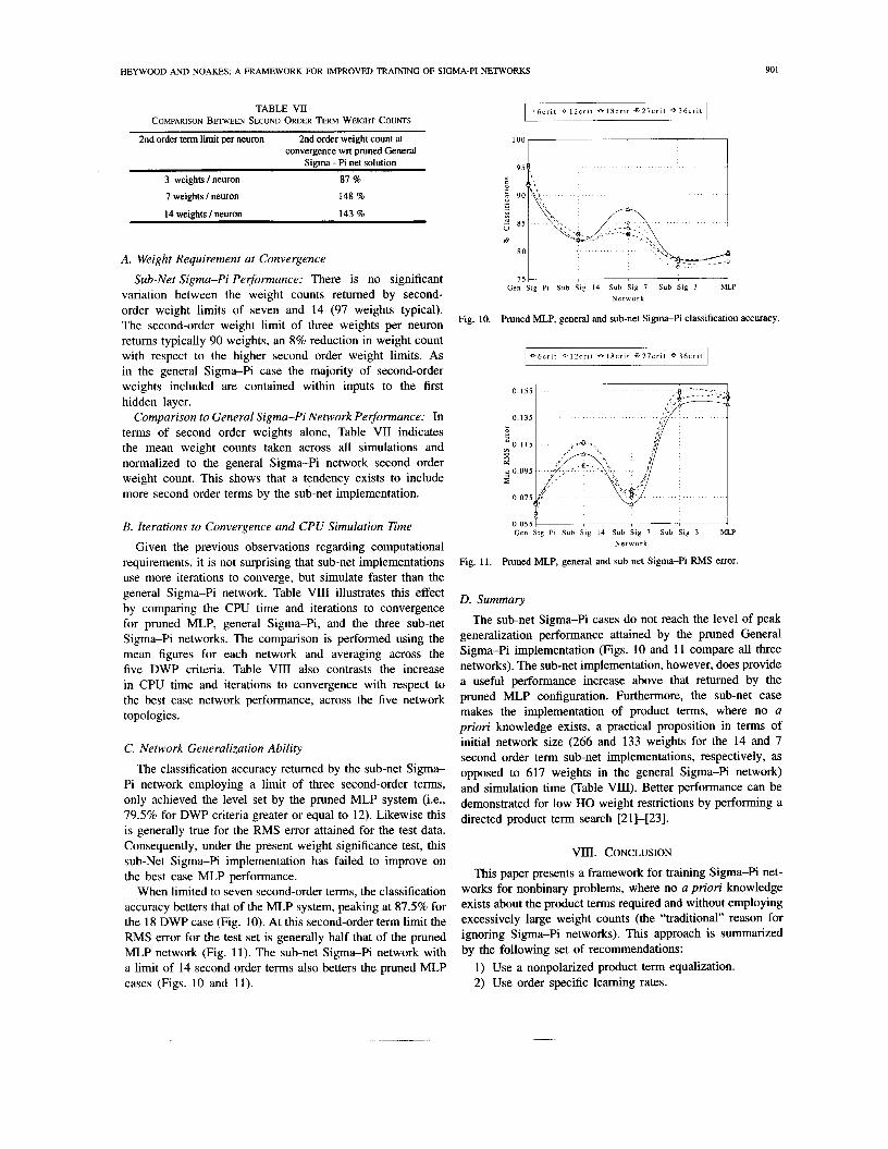
The classification accuracy returned by the sub-net Sigma- Pi network employing a limit of three second-order terms, only achieved the level set by the pruned MLP system (i.e., 79.5% for DWP criteria greater or equal to 12). Likewise this is generally true for the RMS error attained for the test data. Consequently, under the present weight significance test, this sub-Net Sigma-Pi implementation has failed to improve on the best case MLP performance.

When limited to seven second-order terms, the classification accuracy betters that of the MLP system, peaking at 87.5% for the 18 DWP case (Fig. 10). At this second-order term limit the RMS error for the test set is generally half that of the pruned MLP network (Fig. 11). The sub-net Sigma-Pi network with a limit of 14 second order terms also betters the pruned MLP cases (Figs. 10 and 11).

1 a ~ 6 c r i t 0 IZcrit * 1 8 c r i t 3 - 2 7 c r i t Q 3 6 c r i t 1

I Gen Sig PI Sub Sig 14 Sub Sig 7 Sub Sig 3 MLP

N e t w o r k

Fig. 10. Pruned MLP, general and sub-net Sigma-Pi classification accuracy.

I - - 6 c r i t 0 1 2 c r i t * 1 8 c r i t 9 - 2 7 c r i t Q 3 6 c r i t I

0 155

0 1 3 5

2 O O 1 1 5

3 5 0 0 9 5

E

0 0 7 5

0 0 5 5 5 Gen Sig PI S u b Sig 14 Sub Sig 7 Sub Sig 3 MLP

Network

Fig. 11. Pruned MLP, general and sub-net Sigma-Pi RMS error.

D. Summary

The sub-net Sigma-Pi cases do not reach the level of peak generalization performance attained by the pruned General Sigma-Pi implementation (Figs. 10 and 11 compare all three networks). The sub-net implementation, however, does provide a useful performance increase above that returned by the pruned MLP configuration. Furthermore, the sub-net case makes the implementation of product terms, where no a priori knowledge exists, a practical proposition in terms of initial network size (266 and 133 weights for the 14 and 7 second order term sub-net implementations, respectively, as opposed to 617 weights in the general Sigma-Pi network) and simulation time (Table VIII). Better performance can be demonstrated for low HO weight restrictions by performing a directed product term search [21]-[23].

VIII. CONCLUSION

This paper presents a framework for training Sigma-Pi networks for nonbinary problems, where no a priori knowledge exists about the product terms required and without employing excessively large weight counts (the "traditional" reason for ignoring Sigma-Pi networks). This approach is summarized by the following set of recommendations:

1) Use a nonpolarized product term equalization. 2) Use order specific learning rates.


TABLE VIII CPU AND ITERATIONS REQUIREMENT FOR THE THREE NETWORK STRUCTURES

Network Type CPU Simulation Time Iterations to Convergence

Time (mean) difference wrt increase wrt MLP iterations (mean) difference wrt increase wrf MLP Gen. Sigma - Pi Gen. Sigma - Pi

Pruned MLP 137 s reference reference 546 + 250 84 %

Pruned General Sigma - Pi 353 s + 216 s 158 % 296 reference reference

Sub-Net Sigma-Pi : 14 terms 2.51 s + 114s 83 % 310 + 14 5 Yo

Sub-Net Sigma-Pi : 7 terms 197 s + 6 0 s 44 % 363 + 67 26 %

Sub-Net Sigma-Pi : 3 terms 147 s + 1 0 s 7 % 382 + 86 29 %

Implement a subset of the total available product terms. Employ a dynamic weight pruning algorithm to re- move redundant weights, where the higher order terms removed are then replaced by terms not presently available. Extract a sparsely connected network using nondynamic pruning, as convergence approaches. Alter momentum and learning rate as required at sparse network extraction, then complete training using BP alone.

As a consequence of the different nonlinear mapping mechanisms available, it has been shown that differing learning rates are necessary to control the rate of learning for each order employed. A drawback from employing multiple learning rates is that the selection of such terms is a nontrivial problem (here exhaustive simulation could be applied, which is not a practical proposition for large problems). Although as a rule of thumb, to return solutions biased toward the most simple solution, learning rates of HO terms should approximately be an order of magnitude lower than that for first order terms.

To implement higher order systems without employing a priori knowledge about the problem, a randomly selected subset of the higher order weights is used. To employ a larger set of weights than defined by the initial random selection, redundant weights must be identified and replaced by alternative terms during the learning process. This is the function of the dynamic weight pruning framework which is based on two fundamental measures. The first identifies stability, the second weight significance. The stability measure is necessary to determine when the weight values, hence the neuron state, is representative of the present neural target function, as defined by the training process (this state may be transient in nature as the learning cycle progresses). The second, weight significance, identifies how significant a weight is to the objective function (local during DWP, global at sparse network extraction).

The performance returned by the framework falls between that of the fully interconnected Sigma-Pi network, trained with pruning, and the optimally pruned MLP network. Significant reductions in the initial Sigma-Pi network requirements are demonstrated when using the sub-net implementation. This reduction in weight count results in faster simulation times for the sub-net Sigma-Pi implementation with respect to the fully interconnected version. Finally the classification ability

demonstrated by the sub-net implementation is between that of the MLP and general Sigma-Pi networks.

It should be recognized that the definition of our stability measure has an inherent disadvantage in selectivity when weights are replaced. The most recently introduced weights will have a smaller adaptation period than those present from initialization. Consequently, such terms are most likely to be removed should the neuron be re-selected for weight removal. This can be avoided by increasing the selectivity of the stability test to that of each weight by employing individual learning rates for each weight [18], 1311. Such a scheme, however, will introduce further user defined parameters (e.g., permitted range of learning rate variation) and generally make the weight significance estimation more difficult. A better approach, following identification of a redundant product term, would be to avoid perturbing the error surface altogether. To this end replacement product terms are incorporated by

1) Selecting the best fitting product term from a pool of candidates.

2) Initializing the weight and any neural threshold update, so as to minimize the local objective function (i.e., backpropagated error).

/

3) Testing for over fitting of the training set. Such a system has been developed by the authors, as has the incorporation of an OBS weight significance test, within the dynamic weight pruning context [21]-[23]. Further evaluation of the framework performance is currently underway, with extensions to the framework for increasing complexity from a minimal MLP configuration as the network is trained.

REFERENCES

D. E. Rumelhart and J. L. McClelland, Parallel Distributed Processing, Explorations in the Macrostructure of Cognition., vol. 1 . Cambridge, MA: MlT Press, 1986. M. L. Minsky and S. Papert, Perceptrons. Cambridge, MA: MIT Press, 1969. C. L. Giles and T. Maxwell, “Learning, invariance and generalization in high-order neural networks,” Appl. Optics, vol. 26, no. 23, pp. 4972-4978, Dec. 1987. M. I. Heywood, Univ. Essex, Dep. Electronic Syst. Eng., internal progress rep. 1, 1992. T. Maxwell, C. L. Giles, and Y. C. Lee, “Generalization in neural networks: The contiguity problem,” in Proc. Zst IEEE ZJCNN, vol. 2, 1987, pp. 41-46. T. Maxwell and C. L. Giles, “Transformation invariance using high- order correlations in neural net architectures,” in Proc. ZEEE Int. Conf: Syst., Man Cybem., 1986, pp. 627432 . L. Spirkovska and M. B. Reid, “Coarse-coded higher-order neural networks for PSRI object recognition,” IEEE Trans. Neural Networks, vol. 4, no. 2, pp. 276-283, Mar. 1993.


[8] R. W. Duren, “Efficient second order neural network architecture for orientation invariant character recognition,” Ph.D. dissertation, Southern Methodist Univ., Dallas, TX, 1991.

[91 M. I. Heywood, Univ. Essex, Den Electronic Svst. Eng., intemal progress report 2, Sep. 1992.

[IO] C. H. Chang and J. Y. Chaung, “Backpropagation algorithm in higher order neural network,” in Proc. IEEE IJCNN, Baltimore, vol. 3 , 1992, p. 551.

[ l 11 H. Yang and C. C. Guest, “Higher order neural networks with reduced numbers of interconnection weights,” in Proc. IEEE IJCNN, vol. 3, June

[12] V. S . Stometta and B. A. Hubermann, “An improved three-layer backpropagation algorithm,” in Proc. IEEE IJCNN, vol. 2, 1987, pp. 637-643.

[13] M. C. Monzer and P. Smolensky, “Skeletonisation: A technique for trimming the fat from a network via reliance assessment,” in Advances in Neural Network Information Processing Systems. San Mateo, CA: Morgan Kaufmann, 1989, pp. 107-1 15.

[I41 Y. Le Cun, J. S. Denker, and S. A. Solla, ”Optimal brain damage,” Ad- vances in Neural Information Processina Svstems. vol. 2. San Mateo.

1991, pp. 281-286.

CA: Morgan Kaufmann, 1990, pp. 5981605. B. Hassibi, D. G. Stork, and G. J. Wolff, “Optimal brain surgeon and general network pruning,’’ in Proc. IEEE ICNN, San Francisco, vol. 1, 1993, pp. 293-299. S. J. Hanson and L. Y. Pratt, “Comparing basis for minimal network construction with back propagation,” in Advances in Neural Information Processing Systems, vol. 1. San Mateo, CA: Morgan Kaufmann, 1989, pp. 177-185. A. S. Weigand, D. E. Rumelhart, and B. A. Huberman, “Generalization by weight elimination with application to forecasting,” Advances in Neu- ral Information Processing Systems, vol. 3 . San Mateo, CA: Morgan Kaufmann, 1991, pp. 875-882. H. Qin and Z. He, “Variable step BP algorithm which prunes away redundant connections dvnamicallv,” in Proc. IEEE IJCNN. vol. 2. Nov. 1992, pp. 441444.

[19] S. Stalin and T. V. Sreenias, “Vectorised backpropagation and automatic pruning for MLP network optimization,’’ in Proc. IEEE ICNN, San Fransisco, vol. 3, Mar. 1993, pp. 1427-1432.

[20] M. I. Heywood and P. D. Noakes, “Simple addition to backpropagation learning for dynamic weight pruning, sparse network extraction and faster learning,” in Proc. IEEE ICNN, San Francisco, vol. 2, Mar. 1993, pp. 6 2 M 2 5 .

[21] -, “Directed product term selection in Sigma-Pi networks,” in Proc. IEEE ICNN, Orlando, 1994.

[22] -, “Product term selection in a Sigma-Pi framework,” Univ. Essex, Dep. Electronic Syst. Eng., Report No. heywm2, Dec. 1993.

[23] M.I. Heywood, “A Practical Framework for Training Sigma-Pi Net- works with an Application in Rotational Invariant Object Recognition,” Ph.D. dissertation, Dept. Elec. Syst. Eng., Univ. Essex, Colchester, UK, 1994.

[241 D. S. Yang, J. H. Garrett, and D. S. Shaw, “A comparative study of neural networks that can perform transformation invariant pattern recognition,” in Proc. IEEE IJCNN, Beijing, vol. 1, 1992, pp. 664469.

New York Wiley, 1989.

[25] R. J. Schalkoff, Digital Image Processing and Computer Vision.

[26] M.-K. Hu, “Visual pattern recognition by moment invariants,” IRE Trans. Information Theory, vol. 8, no. 2, pp. 179-189, Feb. 1962.

[27] P. Raveendran, S. Omatu, and W. W. Yue, “Performance of generated moments by neural network to recognize invariant image representation,” in Proc. IEEE IJCNN, Beijing, vol. 1, 1992, pp. 6 8 M 9 4 .

[28] M. R. Teague, “Image analysis via the general theory of moments,” J. Optical Soc. Amer., vol. 70, no. 8, pp. 920-930., Aug. 1980.

[29] A. Khotanzad and J.-H. Lu, “Classification of invariant image represen- tations using a neural network,” IEEE Trans. Acoustics, Speech Signal Process., vol. 38, no. 6, pp. 1028-1038, June 1990.

[30] C.-H. Teh and R. T. Chin, “On image analysis by the methods of moments,” IEEE Trans. Pattern Anal. Machine Intell., vol. 10, no. 4, pp. 496-512, July 1988.

[31] A. Estevez Pablo, Okabe Yoichi, “Training the piecewise linear higher order neural network through error backpropagation,” in Proc. IEEE IJCNN, Singapore, vol. 1, 1991, pp. 711-716.

Malcolm Heywood (S’94-M’95) received the B.Eng. degree in electrical and electronic engineering at Polytechnic South West, Plymouth, UK (now University of Plymouth) in 1990, and the Ph.D. degree in neural network system design at the VLSI Research Group at the University of Essex, Colchester, UK, in 1994.

Following a year working at Racal Radar Defence Systems (Leicester) Ltd he joined the Neural and VLSI Research Group at the University of Essex in 1991. His current research interests include time

series analysis, optimization techniques and nonparametric modeling methods. Dr. Heywood is an Associate Member of the IEE.

Peter Noakes (M’94) received the B.Sc. degree from Queen Mary College, University of London in 1967.

From 1967 to 1971 he worked with the Marconi Company in Chelmsford, UK before joining the Department of Electronic Systems Engineering at the University of Essex, where he is now a Senior Lecturer. His research interests include artificial neural networks, signal processing, VLSI digital system design, the application of FPGA’s and computer based learning.

Mr. Noakes has contributed to over 50 conference and joumal publications. He has been on the organizing committees of a number of International FPGA Workshops. He is a member of the IEEE Systems, Man and Cybernetics Society and the IEEE Computer Society. He is also a Chartered Engineer, a Member of the Institution of Electrical Engineers (IEE) and the European Neural Network Society (ENNS).

a framework for improved training of sigma-pi networks...

Documents