a feasibility study of a wi-fi-based vehicular ad hoc
TRANSCRIPT

A Feasibility Study of a Wi-Fi-Based Vehicular Ad Hoc Network in the Westfield Shopping
Mall Parking Lot using Field Trial Measurements and Simulation
by
Foysal Ahmed
A thesis submitted to
Auckland University of Technology
in partial fulfilment of the requirements for the degree of
Master of Computer and Information Sciences
2016
School of Engineering, Computer and Mathematical Sciences
Primary Supervisor: Associate Professor Nurul I Sarkar

ii
Abstract
Vehicular Ad Hoc Networks (VANETs) play an important role in reducing car accidents on the road
as well as in the parking lots of large shopping malls. Providing connectivity as well exchanging
warning messages among the vehicles in the parking areas could potentially reduce car accidents. An
empirical study using radio propagation measurements to get an insight into the performance of a
VANET system in the shopping mall environment is required to assist the efficient design and
deployment of such systems. In this thesis, an empirical investigation using field trial measurements
(i.e. propagation measurements) to study the performance of an IEEE 802.11n-based VANET in the
parking lot of the West City Auckland shopping mall is described and its results are reported. In the
investigation, received signal strength, packet send/receipt and response times were measured
between two experimental vehicles equipped with 802.11n cards. Received signal strengths were
found to have ranged from -45 dBm to -92 dBm in the parking lot. The distance coverage between
two experimental vehicles where warning messages were sent successfully were up to 57 m, 17.5 m,
9.4 m, and 68 m at parking levels 1, 2, 3, and the roadside, respectively. Simulations were performed
to generalize the measurement results. This thesis also investigates a closest match between the
propagation models and measurements. Finally, the thesis provides guidelines for network planners
for the deployment of 802.11-based VANET in the parking lot of a large shopping mall.

iii
Attestation of Authorship
I hereby declare that this submission is my own work and that, to the best of my knowledge and
belief, it contains no material previously published or written by another person, nor material which
to a substantial extent has been accepted for the qualification of any other degree of diploma or a
University or other institution of higher learning, except where due acknowledgement is made in the
acknowledgements.
Signature: ____________________________

iv
Acknowledgements
I would like to thank you my supervisor, Associate Professor Nurul I. Sarkar for his guidance,
discussions and encouragement throughout this research process. His constant enthusiasm and useful
comments were invaluable assistance for me while completing this thesis.
I would to thank to my parents and family (especially my wife) who are always playing an important
role no matter the distance to encourage me during my difficult time.
Finally, I would like to thank the authorities at AUT University for providing the opportunity for me
to finish this research work.

v
Contents Abstract ................................................................................................................................................. ii
Attestation of Authorship ................................................................................................................... iii
Acknowledgements .............................................................................................................................. iv
Contents ................................................................................................................................................. v
List of Abbreviations and Acronyms ............................................................................................... viii
List of Figures ....................................................................................................................................... x
List of Tables ...................................................................................................................................... xiii
Chapter 1 ............................................................................................................................................... 1
Introduction .......................................................................................................................................... 1 1.1 Objective of this study ...................................................................................................................... 3 1.2 Methodology Used for Study ........................................................................................................... 4
1.2.1 Field Trial Measurements (Propagation Measurements) .................................................... 6 1.2.2 Simulation ........................................................................................................................... 7
1.3 Data Collection Process .................................................................................................................... 8 1.3.1 Literature Review Process ................................................................................................... 9 1.3.2 Field Trial Data Gathering Process ..................................................................................... 9
1.4 Thesis structure ................................................................................................................................. 9
Chapter 2 ............................................................................................................................................. 12
VANET and Ad Hoc Networks ......................................................................................................... 12 2.1 Vehicular Ad Hoc Network (VANET) ........................................................................................... 12
2.1.1 Vehicular Ad-hoc Network Communications ................................................................... 12 2.1.2 VANETs applications and classification ........................................................................... 14 2.1.3 VANET’s design issues and challenges ............................................................................ 16
2.2 Mobile Ad Hoc Network ................................................................................................................ 17 2.3 IEEE 802.11 Standard and background .......................................................................................... 18
2.3.1 The IEEE 802.11 Protocols for Vehicular Ad Hoc Network ............................................ 22 2.3.2 IEEE 802.11p Physical Layer ........................................................................................... 23 2.3.3 IEEE 802.11p MAC Layer ................................................................................................ 24

vi
2.4 Wireless mesh network ................................................................................................................... 26 2.5 Wireless communications technology ............................................................................................ 26 2.6 WLAN Signal Strength Measurement ............................................................................................ 28 2.7 Propagation Models ........................................................................................................................ 31 2.8 Summary ......................................................................................................................................... 34
Chapter 3 ............................................................................................................................................. 35
Research Design .................................................................................................................................. 35 3.1 Performance Metric ......................................................................................................................... 35 3.2 Hardware and Software Requirements ........................................................................................... 36
3.2.1 Hardware Equipment ......................................................................................................... 37 3.2.2 Software ............................................................................................................................. 38
3.3 Propagation Measurement Environment ......................................................................................... 39 3.4 Measurement Scenarios .................................................................................................................. 42 3.5 Simulation Environment ................................................................................................................. 44 3.6 Measurement Accuracy ................................................................................................................... 46 3.7 Summary ......................................................................................................................................... 47
Chapter 4 ............................................................................................................................................. 48
Results and Discussion ........................................................................................................................ 48 4.1 Field trial Measurement at West City Auckland shopping mall parking lot .................................. 48
4.1.1 Study 1 (Level 1) ............................................................................................................... 51 4.1.2 Study 2 (Level 1 to Level 2) .............................................................................................. 55 4.1.3 Study 3 (Level 1 to Level 3) .............................................................................................. 59 4.1.4 Study 4 (Level 1 to Level 4) .............................................................................................. 62 4.1.5 Study 5 (Level 1 to Road) .................................................................................................. 62
4.2 Simulation results ............................................................................................................................ 67 4.2.1 OPNET-based Simulation study ........................................................................................ 67
4.3 Summary ......................................................................................................................................... 75
Chapter 5 ............................................................................................................................................. 76
Propagation Models versus Measurements ...................................................................................... 76 5.1 Model Overview ............................................................................................................................. 76
5.1.1 “Free Space” model ........................................................................................................... 77 5.1.2 “Shadowing Path Loss” model .......................................................................................... 77

vii
5.1.3 “Egli” model ...................................................................................................................... 78 5.1.4 “Hata” model ..................................................................................................................... 78 5.1.5 “COST 231” model ........................................................................................................... 79
5.2 Model versus measurement: Comparative study ............................................................................ 80 5.3 Summary ......................................................................................................................................... 86
Chapter 6 ............................................................................................................................................. 87
Implications and Recommendations for System Deployment ........................................................ 87 6.1 Implications .................................................................................................................................... 87 6.2 Recommendations for system Deployment .................................................................................... 89 6.3 Summary ......................................................................................................................................... 92
Chapter 7 ............................................................................................................................................. 93
Conclusions and Future resarch ....................................................................................................... 93 7.1 Summary and Conclusions ............................................................................................................. 93 7.2 Future Reserch ................................................................................................................................ 95
Appendix A : Wi-Fi around West City shopping mall parking lot ................................................ 97
Appendix B : Preliminary Field trials results ................................................................................ 102
Appendix C : OPNET Simulations Configurations ....................................................................... 106
Appendix D : OPNET-based Simulation Scenario Results .......................................................... 108
Appendix E : Model Propagation results ....................................................................................... 110
Appendix F : VANET in the West City Auckland shopping mall parking lot ........................... 115
References .......................................................................................................................................... 119

viii
List of Abbreviations and Acronyms
AP Access Point
AODV Ad hoc On-demand Distance Vector
BSS Basic Service Set
CA Collision Avoidance
CICAS Cooperative Intersection Collision Avoidance Systems Initiative
CPU Central Processing Unit
CSMA Carrier Sense Multiple Access
dB Decibel
dBm dB-milliwatts
DCF Distributed Coordinated Function
DSSS Driving Safety Support Systems
EDCA Enhanced Distributed Channel Access
ESS Extended Service Set
FHSS Frequency-Hopping Spread Spectrum
FSPL Free-space Path Loss
FTP File Transfer Protocol
GPS Global Positioning System
IBSS Independent Basic Service Set
ISM Information Systems Management
IR Infrared
ITS Intelligent Transportation Systems
IVC Inter Vehicular Communications
IWF Information Warning Function
LAN Local-Area Network
LLC Logical Link Control
MAC Medium Access Control
MANET Mobile ad-hoc Network
MH Map Hack

ix
MPDU MAC Protocol Data Unit
mu Microseconds
ms Milliseconds
mW Milliwatts
NLOS Non Line of Sight
OPNET Optimized Network Engineering Tool
P2P Peer-to-Peer
PER Packet Error Rate
PCF Point Coordination Function
PLCP Physical Layer Convergence Protocol
PMD Physical Medium
PHY Physical Layer
OSI Open Systems Interconnection model
QoS Quality of Service
RF Radio Frequency
RSSI Received Signal Strength Indicator
RSU Road Side Equipment
RTS/CTS Request to Send/Clear to Send
RWP Random Way Point
SNR Signal-to-Noise Ratio
SRD Short Range Destination
SSID Service Set Identifier
TCP Transmission Control Protocol
UDP User Datagram Protocol
VANET Vehicular Ad Hoc Network
VCWS Vehicle Collision Warning Systems
V2I Vehicle to Infrastructure
V2R Vehicle-to-Roadside
V2V Vehicle-to-Vehicle
WAVE Wireless Access in Vehicular Environment
WDS Wireless Distribution System
WLAN Wireless Local-Area Network
WMN Wireless Mash Network

x
List of Figures Figure 1.1 Sharing accident information from V2V communication ..................................................... 2
Figure 1.2 Sharing text and downloading multimedia from V2V and RSU communication ................. 2
Figure 1.3: Steps involved in the study ................................................................................................... 5
Figure 1.4: Field trial measurement approach for the study ................................................................... 7
Figure 1.5: Dissertation structure .......................................................................................................... 11
Figure 2.1: Illustration of a vehicular Ad Hoc network ........................................................................ 13
Figure 2.2: VANET applications (Boukerche, Oliveira et al. 2008) .................................................... 14
Figure 2.3: An infrastructure mode ....................................................................................................... 20
Figure 2.4: An ad-hoc network ............................................................................................................. 20
Figure 2.5: Independent Service Set (ISS) ............................................................................................ 21
Figure 2.6: Basic Service Set ................................................................................................................ 21
Figure 2.7: Extended Service Set .......................................................................................................... 22
Figure 2.8: IEEE 802 Family of Protocol’s .......................................................................................... 22
Figure 2.9: IEEE 802.11 Protocol Architecture .................................................................................... 23
Figure 2.10: Wireless LAN MAC Architecture (2003) ........................................................................ 24
Figure 2. 11: Net throughput with 802.11b including RTS/CTS (Prasad and Prasad 2002) ................ 29
Figure 3.1: Photograph showing parking lot of Westfield Shopping Mall Auckland .......................... 40
Figure 3.2: Westfield shopping mall parking layout (A) ...................................................................... 40
Figure 3.3: Westfield shopping mall parking layout (B) ...................................................................... 41
Figure 3.4: Measurement planning sections (A) ................................................................................... 41
Figure 3.5: Measurement planning sections (B) ................................................................................... 41
Figure 3. 6: Measurement planning sections (C) .................................................................................. 42
Figure 3.7: Flowchart field measurement ............................................................................................. 42
Figure 3.8: V2V communications ......................................................................................................... 43
Figure 3.9: OPNET representation of 802.11n model (N = 50) ........................................................... 45
Figure 4. 1: West city Auckland shopping mall parking image ............................................................ 49
Figure 4.2: Number of SSID identified in the West city Auckland shopping mall parking lot ............ 50
Figure 4.3: RSSI (dBm) in West city Auckland shopping mall parking lot ......................................... 50
Figure 4.4: RSSI versus distance coverage ........................................................................................... 51

xi
Figure 4.5: A text file transmission time from TX to RX .................................................................... 52
Figure 4.6: Packets loss in transmission a txt file over distance .......................................................... 53
Figure 4.7: An image file transmission time between TX and RX ...................................................... 54
Figure 4.8: Packets loss in transmission an image file over distance ................................................... 54
Figure 4.9: RSSI versus distance coverage .......................................................................................... 55
Figure 4.10: A text file transmission time from TX to RX .................................................................. 56
Figure 4.11: Packets loss in transmission a txt file over distance ........................................................ 57
Figure 4.12: An image file transmission time from TX to RX ............................................................. 58
Figure 4.13: Packets loss in transmission an image file over distance ................................................. 58
Figure 4.14: RSSI versus distance coverage ........................................................................................ 59
Figure 4.15: An image file transmission time from TX to RX ............................................................. 60
Figure 4.16: Packets loss in transmission a txt file over distance ........................................................ 61
Figure 4.17: RSSI versus distance coverage ........................................................................................ 63
Figure 4.18: A text file transmission time from TX to RX .................................................................. 64
Figure 4.19: Packets loss in transmission a txt file over distance ........................................................ 65
Figure 4.20: An image file transmission time from TX to RX ............................................................. 65
Figure 4.21: Packets loss in transmission an image file over distance ................................................. 66
Figure 4.22: The effect of increasing wireless nods on 802.11 packet delays ..................................... 68
Figure 4.23: The effect of increasing wireless nods on 802.11n throughput ....................................... 68
Figure 4.24: P2P file sharing download file size versus number of nodes ........................................... 69
Figure 4.25: P2P file sharing download response time versus number of nodes ................................. 70
Figure 4.26: P2P file sharing traffic sent versus number of nodes ....................................................... 71
Figure 4.27: P2P file sharing traffic received versus number of nodes ................................................ 71
Figure 4.28: FTP file sharing download response time versus number of nodes ................................. 72
Figure 4.29: FTP file sharing upload response time versus number of nodes ...................................... 73
Figure 4.30: FTP file sharing traffic sent versus number of nodes ...................................................... 74
Figure 4.31: FTP file sharing traffic received versus number of nodes ............................................... 74
Figure 5.1: RSSI versus distance for NLOS condition: Comparison of measurement and five models
.............................................................................................................................................................. 81
Figure 5.2: RSSI versus distance for NLOS condition: Comparison of measurement and five models
.............................................................................................................................................................. 82
Figure 5.3: RSSI versus distance for NLOS condition: Comparison of measurement and five models
.............................................................................................................................................................. 84

xii
Figure 5.4: RSSI versus distance for NLOS condition: Comparison of measurement and five models
............................................................................................................................................................... 85
Figure 6.1: Deployment Scenario - a VANET in the parking lot ......................................................... 89
Figure C1: Application configuration ................................................................................................. 106
Figure C2: Profile Configuration ........................................................................................................ 106
Figure C3: WLAN configuration ........................................................................................................ 107
Figure C4: Simulation result browser ................................................................................................. 107
Figure F1: VANET vehicle with wireless adapter, antenna and laptop .............................................. 115
Figure F2: West City Auckland shopping mall outside parking image .............................................. 115
Figure F3 : West city Auckland shopping mall parking image .......................................................... 116
Figure F4: Frequency range 2.4 GHz in the West City Auckland shopping mall parking lot ........... 116
Figure F5: Frequency range 5 GHz in the West City Auckland shopping mall parking lot .............. 117
Figure F6: Ad Hoc network in the West City Auckland shopping mall parking lot ......................... 117
Figure F7: File sharing, chat through Colligo Workgroup Edition ..................................................... 118

xiii
List of Tables Table 1.1: Credible Resources ................................................................................................................ 9
Table 2.1: VANET applications (Boukerche, Oliveira et al. 2008) ..................................................... 15
Table 2.2: Common 802.11 standards (Perahia 2008). ........................................................................ 19
Table 2.3: Long range wireless technology V2V and V2I communications (Habib, Hannan et al.
2013) ..................................................................................................................................................... 27
Table 2.4: medium range wireless technology V2V and V2I communications (Habib, Hannan et al.
2013) ..................................................................................................................................................... 27
Table 2.5: Comparison between various channel models .................................................................... 32
Table 2.6: Key researcher and their main contributions in Wi-Fi based VANET ............................... 33
Table 3.1: Wi-Fi-Based Vehicular Ad Hoc Network using Field Trial Measurement scenarios ......... 43
Table 3.2: General parameters used in simulations .............................................................................. 45
Table 3.3: OPNET based Ad Hoc Network using multiples of nodes ................................................. 46
Table 4.1: Packets sent and received versus distance for the transmission of an image file from TX
and RX .................................................................................................................................................. 61
Table 4.2: In Ad Hoc network TX and RX communicating between level 1 to level 4 ....................... 62
Table 5.1: Parameters used for models ................................................................................................. 76
Table 6.1: VANET features and implications ...................................................................................... 88
Table 6.2: Smart Antenna technology ................................................................................................. 91
Table A1: Level 1 in West city shopping mall parking lot .................................................................. 97
Table A2: Level 2 West city shopping mall parking lot ....................................................................... 97
Table A3: Level 3 West city shopping mall parking lot ....................................................................... 98
Table A4: Level 4 West city shopping mall parking lot ....................................................................... 99
Table A5: Edsel Street in West city shopping mall parking lot ......................................................... 100
Table B1: Measurement al results Scenario 1 (802.11n) .................................................................... 102
Table B2: Measurement results Scenario 2 (802.11n) ....................................................................... 103
Table B3: Measurement results Scenario 3 (802.11n) ....................................................................... 104
Table B4: Measurement results Scenario 4 (802.11n) ....................................................................... 104
Table B5: Measurement results Scenario 5 (802.11n) ....................................................................... 104

xiv
Table D1: Peer-to-Peer File sharing packet delay (ms) ...................................................................... 108
Table D2: Peer-to-Peer File sharing Throughput (kbps) .................................................................... 108
Table D3: Peer-to-Peer File sharing traffic received (kbps) ............................................................... 108
Table D4: Peer-to-Peer File sharing traffic sent (kbps) ...................................................................... 108
Table D5: Peer-to-Peer File download file size (mbps) ...................................................................... 108
Table D6: Peer-to-Peer File download response time (sec) ................................................................ 108
Table D7: Ftp download response time (sec) ...................................................................................... 109
Table D8: Ftp upload response time (sec) .......................................................................................... 109
Table D9: Ftp traffic received (kbps) .................................................................................................. 109
Table D10: Ftp traffic sent (kbps) ....................................................................................................... 109
Table E1: Scenario 1. Measurement data under Non-LOS Conditions .............................................. 110
Table E2: Scenario 2. Measurement data under Non-Los Conditions ................................................ 111
Table E3: Scenario 3. Measurement data under Non-Los Conditions ................................................ 112
Table E4: Scenario 4. Measurement data under Non-Los Conditions ................................................ 112
Table E5: Scenario 5. Measurement data under Non-Los Conditions ................................................ 112

1
Chapter 1
Introduction
The number of automobiles on the road has been increasing rapidly over the last 10 years. Every year
on U.S. highways there are about 43,000 accidents, 6.3 million police-reported traffic accidents and
millions of people are injured. The economic effects are more than $230 billion caused by accidents
and traffic delays resulting from vehicles leaving the road or travelling dangerously through
intersections (Hassan 2009). At this time traffic congestion on the roads is a superior issue in crowded
cities. The congestion and vehicle related problems such as bad traffic jams, slow or fast driving, not
giving way to emergency vehicles and poor road conditions are accompanied by a constant threat of
accidents. VANETs (Vehicular Ad-hoc Network) are a possibility for future vehicle applications
(Raya and Hubaux 2007). VANET is, as the name implies, an ad-hoc network with digital
communications vehicle to vehicle: a point-to-point wireless network (dedicated server) whose nodes
are devices placed in vehicles. VANET is a subset of MANETs which is more advanced applications
technology that offers ITS in wireless communication between V2V and RSU to vehicles according
to IEEE 802.11p standard. Ad hoc networks are the category of wireless networks that uses multi hop
radio relaying. Wi Fi technology is targeting to equip technology in vehicles to decrease these issues
by sending messages to each other. Recently researchers have been focusing their efforts on
improving road safety by new developments in latest vehicular technology and the evolution of
wireless technology has allowed vehicles to participate in the communication network
The main objective of VANET is enhancing safety and efficiency in transportation systems, which
communicate and provides a long list of applications varying from transportation protection to driver
support and Internet access. Figure 1.1 shows sharing information V2V which provides collision
detection, lane change warning, electronic brake warning, audio/ video exchanging, route guidance,
weather information, electronic payment, internet access, post-crash notification, intersection
violation warning, on-coming traffic warning, vehicle stability warning and traffic signal violation
warning.

2
Figure 1.1 Sharing accident information from V2V communication
Figure 1.2 Sharing text and downloading multimedia from V2V and RSU communication
Sometimes driver behavior on the road is extremely complex as drivers react to challenging road
conditions depending on their plans and behavior (Naumov, Baumann et al., 2006). Figure 1.2 shows
V2V sending test messages and downloading multimedia from RSU. Applications can provide drivers
additional information on traffic situations which will react timely and correctly assess possible risks.
Adding an extra value in the operations services and vehicle industries, VANET might be considered
as a future killer application. It is very confusing on motorways or highways to predict and monitor
other drivers’ speeds. However, with computer and wireless communication or sensor equipment,
speeds could be monitored and the risk of potential accidents could be minimized by sending a
warning message. This kind of network facility will generally be used to allocate safety message

3
information such as traffic significant information, collision warnings and risk warnings.
To reduce accidents, Vehicular Ad-hoc Networks (Lagraa, Yagoubi et al., 2010) have been
developed by network researchers to provide added safety for all vehicles on the road. To improve the
safety, security and efficiency of transportation systems, ITS have been developing vehicle and
transportation infrastructures that apply rapidly emerging information technology. Information
Warning Function (IWF) would be used to warn the vehicle of the possibility of any danger on the
road and inform the driver to take defensive action. The main challenges in VANET operation are the
frequent changes in network topology due to the high mobility of the network nodes. IEEE 802.11
(Wi-Fi) based VANETs are becoming an attractive solution for road safety because of their low cost,
widely used standards and mobility offered by the technology. In 802.11 transmissions the distance
between the sender and receiver is an important factor causing decrease of performance for poor
latency and throughput due to inefficiencies in implementation of the vehicular networking stack. Still
there are some challenges and issues with VANET such as lack of online management, radio channel,
high mobility, environmental conditions, security and privacy.
1.1 Objective of this study
The objective of this research was to conduct a feasibility study for the deployment of IEEE 802.11-
based VANET in the parking lot of West City Auckland shopping mall. The idea is to set up a
VANET in the parking lot to measure the system performance in terms of received signal strengths
and response time. To fulfill this objective, a field trial propagation measurement was conducted
using 802.11n cards. To generalize the measurement results, OPNET-based simulation was
performed. In this thesis the following research questions have been addressed:
• What guidelines can be provided for network planners to implement an IEEE 802.11-
based VANET in the parking lot of a large shopping mall?
• What propagation model would be the best-fit (closest match) with the measurement results?

4
1.2 Methodology Used for Study
"A methodology is a set of guidelines or principles that can be tailored and applied to a specific
situation. In a project environment, these guidelines might be a list of things to do. A methodology
could also be a specific approach, templates, forms, and even checklists used over the project life
cycle" (Charvat, 2003). Selecting the appropriate methodology is the best justification for reducing
risk, reducing cost, avoiding mistakes, identifying earlier errors and meeting project schedules. Case
and Light (2011) specified there are three comprehensive types of methodology used to manage a
research study: qualitative research, quantitative research and mixed method research. Quantitative
research involves gathering numerical data and using mathematical-based techniques to clarify
phenomena or research questions (Lindsay 2005). Quantitative methods also provide some strength
including: suitable for studying huge numbers of people and experiments; quantitative research is
subjective; quantitative method is comparatively fast for data collection; can generalized as research
findings; testing and validating already constructed theory; data analysis is relatively less time
consuming; provides quantitative, precise numerical data.
In quantitative research there are two main types of design: experimental design and non-
experimental design. Experimental methods contain accurate experiments, which are a random
assignment of subjects to treatment conditions. Zahn, O'Shea et al. (2009) established a V2V test bed
experiment with emphasis on assessing the quantity of data that could be transferred among two
moving vehicles and a fixed access point in urban and highway scenarios. However, similar
experiences with other vehicle test beds have been presented by others but all have the same recurring
problem: limited availability of equipment (Amoroso, Marfia et al., 2012). Moreover, experimental
methods have their own drawbacks. They are normally expensive to implement and are not
cooperative to extrapolation.
We used the quantitative approach and all data used in the analysis process were data collected
from field trial measurements, OPNET simulations as well as simulation methods. The study adopted
field trial measurements to get an insight into the performance of VANET in the shopping mall
parking environment. Moreover, OPNET-based simulation is conducted to generalize the field trials
measurement results. Simulations of VANETs often involve large and heterogeneous scenarios. There
are two main components in a VANET network: a component that is capable of simulating the
behavior of a wireless network, and a vehicular traffic component that is able to provide an accurate
mobility model for the nodes of a VANET.

5
Figure 1.3: Steps involved in the study
Modified design science methodology was adapted in this study as the most appropriate model for
this research. This model is based on sequential steps to carry out research and is a linear approach to
software development which gathers and documents requirements, design and performance study.
Also, this model is useful when the requirements are clear, well-known and fixed, short projects and
there are no ambiguous requirements. This model contains certain advantages: it is very simple to
implement, each stage produces documentation for development, easier to detect and diagnose faults
at an early stage. Figure 1.3 shows all stages and steps involved in measurement /field trials.
Phase 1: This phase involves the express area of interest, outlines the existing problems and
identifies goals to be achieved after the problem is solved. Supervisor guideline and
discussion occurs in this phase.
Phase 2: This phase describes a review on past study with all relevant works to support this
study.
Phase 3: This phase involves requirements for measurement, which includes hardware setup,
software installation and design.

6
Phase 4: This phase provides quantitative data generated and various outputs captured, for
example frequency, test scores, test result, number or percentages.
Phase 5: In this phase all data collected from earlier phases are analyzed and compared using
suitable tools, for example Microsoft Excel.
Phase 6: This phase provides system implication based on earlier phases.
Phase 7: This is the final phase, based on all phase conclusions. The supervisor needs to
provide feedback depending on this study.
1.2.1 Field Trial Measurements (Propagation Measurements)
Field trial testing generally focused on checking the feasibility of Wi Fi connections among vehicles
in a shopping mall parking area. Field trial experimental measurement provides a difference to
validate the results of analytical modeling and computer simulation to check the accuracy of the
WLAN study. The most important aspects in this study that we considered while carrying out these
tests are the hardware for Wi Fi communication and measuring distance of both vehicles using a
correct method. On the test the driver must be aware of the positions where vehicles are parked and
move into Wi Fi range.
Figure 1.4 illustrates the methodology used for this study. Each scenario of field trial design starts
with defining the propagation measurements in the entire project. The next process consists of
defining routes where V2V can communicate for propagation measurements. The following steps are
route measurements with 1m distance making sure V2V is connected with the ad hoc network. The
next process contains primary trials in order to recognize that the parking area can be measured. If the
parking area consists of too much interference then we need to go to another parking area. Each
scenario was designed with two trials to measure the accuracy of the Wi-Fi connection through a pair
of nodes. The next procedure involving data collection and validation is compiled and performed.
Finally a comparative analysis is done and conclusions discussed.

7
Figure 1.4: Field trial measurement approach for the study
1.2.2 Simulation
There are two types of simulators for smooth functioning in VANET: network simulators and traffic
simulators. Network simulators are generally used to evaluate network applications and protocols in
particular conditions. Traffic simulators are typically used for traffic engineering and transportation.
Moreover, a VANET simulator is a combination of a network simulator and a large number of traffic
simulators. However, most of the VANET simulators have a problem of proper ‘interaction’.
Mangharam, Weller et al. (2005) produced the first tools for assessment of VANET performance for
forecasting and vehicular traffic flow. Numerous communicating network simulation tools already
offer a platform to test and evaluate network protocols, for example NS-2 (Andr, Varga et al. 2008),
OPNET (Weingartner, vom Lehn et al. 2009) to provide several models of switches, routers and
servers based on vendor specifications. However, simulation tools are designed to deliver general
simulation scenarios without being specifically adapted for applications in the transportation

8
atmosphere. Advanced level simulation software has struggled to obtain detailed operational features
of network protocols. Simulation tools are not enough for a comprehensive study of WLAN in
numerous aspects and analytical modeling has a tough road in analysis of TCP over multiple-hop
WLANs (Jin, Seung-Keun et al. 2003). OPNET can be used as a platform to develop models of
a wide range of systems such as internetwork planning, LAN and WAN performance; mobile
packets radio networks and satellite networks. It also provides a wide-ranging development
atmosphere for modeling and performance evaluation of communication networks and
distribution systems. Specification, data collection and simulation, and analysis phase
modeling are major categories in OPNET and are performed in sequence. OPNET modeling
efforts obtain measures of a system’s performance or make observations concerning a
system’s behavior and admit realistic approximations of performance and behavior to be
obtained by executing simulations. There are some advantages to using OPNET such as cost
and time, efficiency and easy to reuse and modify scenarios. OPNET has increased significant
acceptance in both academia and industry by providing a number of model networks that are
commercially presented network mechanisms. However, there is no proper method for
organizing VoIP or video conferencing into a current network in OPNET and it also requires high
PC specifications and consumes big amounts of memory (Hussain and Habib 2011).
1.3 Data Collection Process
Data collection process was used in this section to obtain the data for this study. Quantitative methods
contain the collection of data so the information can be counted and subjected to statistical analysis.
The quantitative method also includes data collection in usually numeric and mathematical models,
which researchers manage to use as the methodology of data analysis. There were two types of data
collection methods used in this research: literature review and measurement data gathering process.
The literature review process provides a knowledge base and information required for this study. In
terms of field trial measurements all data gathering processes were carried out using multiple tests in
the shopping mall parking center.

9
1.3.1 Literature Review Process
A literature review is the initial process of objective analysis, through a summary and critical analysis
of others’ relevant works. The main goal of the reader is to update with current literature on a chosen
topic such as justification, limitations and future research area. A good literature review also provides
the background of the study, knowledge base, clear search, selection strategy and information
required for this study.
In this study, all literature was collected from different reliable resources, for example academic
databases, books, library references and a proper reliable association website. Table 1.1 shows an
example of reliable resources. After the literature is reviewed and critically analysed, the next process
is measurement and data gathering.
Table 1.1: Credible Resources
Resources From
Academic database IEEEXplore, EBSCO HOST, ACM Digital Library, ScienceDirect Journal Database
Books AUT library, Google Books
Web search engine Google scholar
1.3.2 Field Trial Data Gathering Process
This section is the main resource for data gathering for this study. Data collection was done from
WirelessMon software. To achieve this data gathering process, two computers with ad hoc networks
were set up in the Henderson Westfield Shopping mall parking lot and numberous tests were run in
order to get accurate results.
1.4 Thesis structure
Figure 1.5 shows the structure of the dissertation. This study consists of seven chapters. Chapter 1 and
Chapter 2 present background material. Chapter 3 to 6 combine to make the main contribution and the
final chapter presents concluding remarks.

10
Ø Chapter 1 – Introduction: This chapter provides an introduction to the thesis and
motivation for undertaking the research. It also covers the methodology employed for this
research with real measurement and analytical methodologies.
Ø Chapter 2 - Vehicular Ad-Hoc Networks: Reviews related work on Vehicular Ad-Hoc
Network’s challenges and issues in wireless propagation measurements. This chapter
describes the IEEE 802.11 standard with the IEEE 802.11p physical layer and MAC layer.
Ø Chapter 3 – Research design: Describes details of experiential design used for this study,
which are hardware and software requirements. The propagation measurement environment
and preliminary propagation field trial measurement scenarios are described.
Ø Chapter 4 – Results and discussion: The findings from propagation measurements are
presented.
Ø Chapter 5 – Propagation models versus measurements: This chapter covers a
comparison of the model implementation’s results with measurement data.
Ø Chapter 6 – Implications and recommendations for future systems deployment: This
chapter discusses the practical implications in future VANET environments.
Ø Chapter 7 - Conclusions and future research: Summarises each chapter and presents the
overall findings made by the study.

11
Figure 1.5: Dissertation structure

12
Chapter 2
VANET and Ad Hoc Networks Chapter 1 outlined objectives of the thesis and thesis stature and presented the methodology used for
study. The key network researchers and their main contributions to the design and fundamentals of
VANET networks are identified and discussed in Chapter 2. Section 2.1 describes a vehicular Ad Hoc
Network based on IEEE 802.11 wireless technology as well VANETs applications and classification
and VANET’s issues and challenges. Section 2.2 outlines the MANAT network where nodes
represent vehicles moving at high steps and vehicle traffic persistent consistency. Section 2.3 outlines
and compares the development and properties of the IEEE 802.11 b,a,g and n standards. This section
also provides details of IEEE 802.11p protocols for vehicular Ad Hoc Network. Section 2.4 outlines
wireless mesh clients and mesh routers. Section 2.5 explains wireless communications technology
classified according their range and differentiates long range, medium range and short range. Section
2.6 outlines WLAN signal strength management with WLAN performance, IEEE 802.11 signal
strength and indoor positioning systems. Section 2.7 outlines propagation measurement models.
2.1 Vehicular Ad Hoc Network (VANET)
2.1.1 Vehicular Ad-hoc Network Communications
Vehicular Ad Hoc Network (VANET) is accepted as an important constituent of Intelligent
Transportation Systems. The key advantages of VANET communication are in active safety
communications and the object of VANET is to increase safety of drivers and passengers by
exchanging information between V2V. VANETs are an extreme case of MANETs. In MANETs,
nodes connect with each other in an ad hoc mode, for example, without attached infrastructure. Nodes
communicate in VANET in similar ways, however the network topology changes frequently with
high speed and different mobility features such as all vehicles in VANET are moving within specific
directions. Tufail, Fraser et al. (2008) tested the existing Wi-Fi protocol for Vehicle-to-Vehicle
(V2V) communication particularly at high speed with several protocols (V2R and V2V). As a result

13
they demonstrated with real-life measurements and logical justification that Wi-Fi is a successful way
of communication between vehicles even at extremely high speeds and also suggested some useful
applications. Moreover VANET provides massive chances and opportunities in online vehicle
entertainment such as through the local ad hoc networks sharing pictures, video, files, gaming and
chatting. Figure 2.1 shows this kind of technology used to communicate in vehicle roadside sensors,
positions, intersection maps and both way wireless communications.
Figure 2.1: Illustration of a vehicular Ad Hoc network
This kind of network usage communication kit exchanges messages with each other in Vehicle-to-
Vehicle (V2V) and it also exchanges messages with a Vehicle to Infrastructure (V2I) and roadside
network infrastructure (Vehicle to Roadside Communication V2R). Figure 2.2 shows this network. A
number of applications have already been proposed which are likely designed for some vehicles
recently such as safety monitoring, map localization, parking lot localization, security distance
warning, vehicle-to-vehicle communication, platooning, vehicle collision warning systems,
cooperative intersection safety, internet access, driver assistance etc. (Boukerche, Oliveira et al. 2008)
.

14
Figure 2.2: VANET applications (Boukerche, Oliveira et al. 2008)
VANET apply short-range communication based on IEEE 802.11 wireless technology, which is
multi-hop communication using geographic positions enabling exchange information between
network nodes. VANET’s knowledge of the present position of nodes is an assumption made by most
algorithms, protocols and applications, for example, since GPS receivers can be easily installed in any
vehicle or be already built within the technology of the car. For an assumption, since GPS receivers
can be installed easily in vehicles, a number already come with this technology. GPS has some
undesired difficulties; for example, not continuously being available or losing signal or not being
robust or sufficient for certain applications. Although VANETs progress is hooked on critical areas it
is gradually becoming connected to local systems.
2.1.2 VANETs applications and classification
The principle determination of communication in vehicular networks, whether in vehicle-to-
vehicle or vehicle-to-infrastructure, is to offer safety and/or non-safety assistance. VANET
applications are categorised into two groups: message and file delivery (target receivers with
acceptable performance, accident and road construction warning systems, priority over non-safety
applications), and internet connectivity (vehicles can communicate to roadside Internet gateway via
the ad hoc network Group (2010). Moreover, the safety application is given main priority in VANET.
However, transmission collision may occur due to a transmission of other safety messages, for
example, alternative safety messages that need to be sent with priority at the same time. A
number of applications involving VANET can take some advantage of localization techniques.
However, identifying their physical location is difficult among nodes such as longitude, latitude and

15
altitude or virtual spatial distribution relative to each other. For example, map location is generally
completed using GPS receivers with a Geographic Information System, although VCWS can be
applied by comparing distances among nodes’ locations combined with geographic information
distribution. Driverless vehicles and VCWS advance toward more critical applications in VANET
technology but they will require a robust and highly offered localization system. GPS accuracy range
is up to 20 meters or 30 meters and not able to work indoors or city areas because they do not have
direct visibility to satellites. Inappropriately, it is not the best solution for VANET applications.
Although other applications such as particularly critical safety applications require more reliability
and accuracy for localization systems with sub-meter accuracy. For security reasons GPS information
is probable to be joined with other localization techniques, for example cellular localization, dead
reckoning and image/video localization. VANET applications do not require localization to function.
When the position of the vehicle is available then it can take advantage of localization for showing
better performance (Table 2.1).
Table 2.1: VANET applications (Boukerche, Oliveira et al. 2008)
These kinds of networks rely on the use of short range networks (about 100 meters) with IEEE 802.11
for vehicle communication and providing bandwidth in the range of MBPS. Drivers can send and
receive information from nearby drivers using VANET. Drivers can exchange information with other
Technique Localization Accuracy
Low Medium High
Routing
Data Dissemination
Map Localization
Coop. Adapt. Cruise Control Coop. Intersection Safety
Blind Crossing
Platooning
Vehicle Col. Warn. System Vision Enhancement
Automatic Parking
Vision enhancement
Automatic parking
X
X
X
-
-
-
-
-
-
-
-
-
-
X
X
X
X
-
-
-
-
-
-
-
-
-
-
X
X
X

16
drivers in communication networks such as when a possibly dangerous incident arises (emergency
braking, accident, suddenly stopped vehicle, speeding) difficult traffic conditions. Specifically, some
other networks have addressed the advertisement of available parking spaces and finding an available
parking space is certainly stressful. Moreover, it indicates environment pollution and fuel
consumption due to the release of gases. Caliskan, Graupner et al. (2006) presented the costs of
searching for parking spaces and also expressed closely two cars on the move searching for a parking
area. To find out advertised available parking space on a parking lot Xu, Ouksel et al. (2004) used the
following significance function to characterise the relevance of a parking space.
2.1.3 VANET’s design issues and challenges
Nzouonta, Rajgure et al. (2009) presented actual issues and challenges of VANET applications in
V2V communication, for example, hidden and exposed mode problems, fake message send, stability,
scalability, reliability and security. One of the main issues is high speed and frequent topology change
when vehicles move very fast within the vehicular network. While, due to road geometry, vehicles
guidelines can be predicted to a certain area, these issues might be treated very carefully by the MAC
protocol; such as if the transmission ranges of two nodes communicate with each other. However, the
system’s performance can be degraded intensely due to high speed (when vehicles move 110km or
140km having frequent link disconnections arising) and high node density. Scalability is another
issue, which is vehicle density, is almost the average, such as changes of network. While the vehicle
density can quickly grow significantly and becomes very large in a road segment without suffering a
noticeable detriment in performance or a complexity increment. Hidden and exposed node problems
are one of the main issues in VANET. Because of the high speed mobility in vehicular networks, the
hidden node problem is predicted to occur more frequently. Yihong and Nettles (2005) proposed this
problem could be solved by using the request-to-send/clear-to-send (RTS/CTS) handshaking. Ho,
Leung et al. (2012) classified VANET simulations as macroscopic or microscopic. They also
explained network component and vehicular traffic component in a VANET simulator, which
provides capability of wireless network behavior and presents an accuracy mobility model of nodes of
VANET.
Liu, Khorashadi et al. (2010) conducted research about assessing VANETs under different traffic
mobility, which is both one-way and highway free flow traffic. Firstly they examined city traffic with
a Random Way Point (RWP) mobility model and finally they performed simulations based on real
traffic trace. Karim (2008) proposed VANET would be the main comfort and safety related

17
application for car and passenger safety. However security and privacy issues will occur with these
applications, such as fake messages, private information etc. Also the author explained why VANET
is better than 3G due to infestations. Many researchers have studied VANET to change the random
directions – the random way where the nodes change the speed and direction randomly (Naumov,
Baumann et al. 2006). The researchers compared ad-hoc Wi-Fi in VANET with real experience
versus simulated where real-world communication was quite hard to simulate due to complexity of
wireless transceivers. To improve the traffic efficiency requires traffic lights and vehicle
communication. To set up VANET might require very expensive infrastructure however it will
require low maintenance costs. Also, there is no associated cost for small-range wireless
communication technologies except the communication devices.
However, VANETs can be vulnerable to attacks and threaten users’ privacy. Hubaux, Capkun et
al. (2004) address the security and privacy challenges in VANET. Others researchers have provided
threat analysis and suggest security architecture based on public key cryptography. Yamamoto,
Ohnishi et al. (2008) proposed the DSSS to prevent accidents by warning drivers about possible
threats at intersections and their main target for DSSS was red light violations, crossing-path
accidents, stop sign violations, turning accidents and collision with pedestrians. Intersection safety
proposed in CICAS implements wonderful safety applications merging with different ITS
technologies, such as decreased intersection accidents by directing real-time warnings together at the
infrastructure and vehicle.
2.2 Mobile Ad Hoc Network
MANET is a wireless mobile node that accommodatingly forms a network without infrastructure. Ad
hoc networks are the highest development of wireless networks and VANET has extensively
reviewed this area of wireless communication at present. VANET is a subsection of MANET where
nodes represent vehicles moving at high step and vehicle traffic persistent consistency. Mobile Ad
Hoc Networks are constructed on wireless links and will remain of significantly inferior capability
than wired counterparts. MANET networks physical security is limited due to the wireless
transmission. VANET shares certain similar characteristics with common MANET. The movement
and self-organization of the nodes characterize together MANET and VANET. MANET finally used
a peer-to-peer network for the exchange of data or channel through speech.
However, MANET involves numerous nodes that cannot recharge their power and have un-
controlled moving patterns but often VANET nodes can charge. MANET has several challenges such

18
as resource issues, wireless communications issues and routing packets where the topology is often
changing (Conti and Giordano 2014).
2.3 IEEE 802.11 Standard and background
In 1997 the IEEE 802.11 standard was first published. IEEE 802.11 consists of a low data rate of 1
Mbps to 2 Mbps and operates at 2.4 GHz ISM band. In 1999, the IEEE 802.11 committee approved
IEEE 802.11a and 802.11b amendments. The standard employs frequency-hopping spread spectrum
(FHSS) and direct-sequence spread spectrum (DSSS) techniques for radio transmission. IEEE 802.11
based wireless access technology has widely been used in WLAN. WLAN technology has two
(managed and uncoordinated) possible development infrastructures in IEEE 802.11 networks. WLAN
technology can deliver high-speed Internet connectivity up to 11 Mb/s (IEEE 802.11b) or 54 Mb/s
(IEEE 802.11a/g). Woesner, Ebert et al. (1998) presented two wireless LAN standards, which are
IEEE 802.11 and HiperLAN in simulations of power saving mechanisms. They also demonstrated
various size beacon intervals in IEEE 802.11 have major impacts on throughput.
IEEE 802.11b supports a bandwidth of 5.5 to 11 Mbps and uses the same unregulated radio
signaling 2.4 GHz frequencies and outdoors cover around 35 to 140 meters. Every channel requires
the same 11-MHz bandwidth as an 802.11 DSSS channel. However, IEEE 802.11b speed is slow.
IEEE 802.11a is a second extension and it is much faster than IEEE802.11a. Actually IEEE 802.11b
and IEEE 802.11a were created at the same time. IEEE 802.11 supports a bandwidth of up to 54
Mbps and uses 5 Ghz frequency spectrums. However, possible data rates per channel for IEEE
802.11a are 6, 9, 12, 18, 24, 36, 48, and 54 Mbps. An IEEE802.11g supports a network bandwidth of
12 to 54 Mbps and uses 2.4 Ghz frequencies for a better range. Signal range is good and not easily
obstructed; however appliances may delay on the unregulated signal frequency. IEEE 802.11n
supports a network bandwidth up to 3000 Mbps. It also offers better signal range over earlier Wi-Fi
standards. It supports multiple wireless signals and antennas and also is more resistant to signal
interference from outside sources. Indoor coverage for IEEE802.11n is approximately 70 meters and
outdoor ranges 250 meters. However, multiple signals interfere with nearby networks (Perahia 2008).
IEEE 802.11ac supports a network bandwidth up to 450 Mbps on 2.4 GHz. It utilizes dual band
wireless technology and its covered backward compatibility to 802.11b/g/n as shown table 2.2

19
Table 2.2: Common 802.11 standards (Perahia 2008).
Standard Frequency band (GHz)
Bandwidth (GHz)
Approximate Range (m)
Maximum data rate (Mbps)
Number of channels
Ad-hoc ability
802.11b 2.4 20 140 11 3 Yes
802.11a 5 20 120 54 23 Yes
802.11g 2.4 20 140 54 3 Yes
802.11n 2.4, 5 20, 40 250 600 26 Yes
Ghahfarokhi (2015) mentioned IEEE 802.11 has a lack of proper channel assignment generally
because of unawareness of users about its importance. The IEEE 802.11 standard has two types of
scanning modes: passive and active. In the passive scan mode, MH listens to each channel of the
physical medium consecutively and tries to locate the next AP and deliver the MH through timing and
advertising information. So the passive scan mode experiences significant delay. The active scanning
mode contains the transmissions of investigation request frames by the MH, which is collecting the
information from all presented APs. IEEE 802.11 technology exploits unlicensed frequency bands of
2.4 GHz or 5 GHz where 2.4 GHz band is more popular. However 2.4 GHz band contains 1 to 14
channels but 3 channels (1, 6, and 11) are non-overlapping. Although 12 channels in the 5 GHz band
are non-overlapping (Chieochan, Hossain et al. 2010), Bisdikian (2001) proposed a Bluetooth device
with low-cost and low power in the wireless network, which is organized into Piconets and it consists
of up to seven slave devices.
The IEEE 802.11 networks standard supports two common operation modes: ad-hoc mode and
infrastructure mode. In infrastructure mode all clients communicate with each other wirelessly and
wired through a wireless AP (as shown in figure 2.3). The stations need to be connected to an AP in
the network in order to communicate to each other. A wireless AP which supports one or many
wireless clients is recognized as BSS. When two or more wireless APs are connected to a similar
wired network it is recognized as ESS.

20
Figure 2.3: An infrastructure mode
Figure 2.4 shows an ad-hoc mode wirelessly communicating directly with each other without using an
access point. The ad-hoc mode is able to connect or communicate wirelessly when there is no
wireless AP present or the wireless client is obviously configured to use the ad hoc mode or AP
discards a connotation due to failed authentication.
Figure 2.4: An ad-hoc network
IEEE 802.11 network architecture consists three different types of network: (Group) basic service set
(BSS); (Group) independent BSS (IBSS); and extended service set (Dressler, Sommer et al.). BSS (as
shown in figure 2.6) is a set of stations that communicate with each other and contains more than two

21
wireless nodes. BSS does not usually indicate to a specific area due to the uncertainties of
electromagnetic propagation and also BSS no longer communicates sprightly in all stations;
consequently AP acts as a master to control the station. IBSS (as shown in figure 2.5) is IBSS is
usually a short-lived network, with smallest number of service station units, which is created for a
particular purpose in the IEEE 802.11 network. IBSS can enable communication with other wireless
stations without AP. However, if a group of mobile terminals transfers data through wireless media
then all nodes need to be within signal range of each other, and if any node is out of signal range they
cannot communicate and are not able to share anything, therefore topology is referred to IBSS or also
recognized as ad hoc (Mishra, Shin et al. 2003) .
Figure 2.5: Independent Service Set (ISS)
Figure 2.6: Basic Service Set
An extended service set (as shown in figure 2.7) network appears similar to an LLC layer as an IBSS
network. BSS to another transparently to LLC may move ESS stations to communicate. The SSID
component specifies the identity of an ESS or IBSS. The ESS distribution system shares and
communicates through wireless stations and APs from same LLC layer.

22
Figure 2.7: Extended Service Set
2.3.1 The IEEE 802.11 Protocols for Vehicular Ad Hoc Network
Protocol architecture 802.11 is a member of the IEEE 802 family. In IEEE 802.11p is one of the
present approved amendments to the IEEE 802.11 standard to add in WAVE. Figure 2.8 shows the
connection between different components of the IEEE 802.11 and IEEE 802 families and their
position in the OSI model. The IEEE network has different types of layers, which is IEEE 802.11
standard specifications focused for the two bottom row made up levels in the OSI Model networking
stack: the Physical Layer and the Medium Access Control. Also it introduces how IEEE 802.11 fits
with existing IEEE 802 also IEEE 802 network has both PHY and MAC components. The LLC and
MAC layer combination can be connected to the OSI model as the data link layer. While IEEE
802.11a, IEEE 802.11b, and IEEE802.11g adopt verities of physical layers for sharing common MAC
and LLC through the same link layer address (48-bit).
Figure 2.8: IEEE 802 Family of Protocol’s

23
2.3.2 IEEE 802.11p Physical Layer
IEEE 802.11 PHY is the interface between the wireless and MAC layer where this layer frames the
receive and transmit data frame. As shown in Figure 2.9 the physical layer of the OSI architecture is
comprised of two separate sub layers which are (Group) physical layer convergence procedure
(PLCP); and physical medium dependent (PMD). The physical medium dependent sub layer
interfaces straight to where the wireless transmission medium frames occur of modulation and
encoding/decoding of the transmission. The physical medium dependent key responsibility is to
include bit-timing, signal coding and interacting with a physical medium. The MPDU framing system
is appropriate for sending/receiving user data and management data among those linked with PMD
system physical frame delivery. The IEEE 802.11 physical layer connects via transient data primitives
between the PLCO and PMD sub layers. PLCP sub layer maps the MPDU framing system
appropriately for sending or receiving management data and user data among related PMD systems
for PHY frame delivery (Bing 1999).
Figure 2.9: IEEE 802.11 Protocol Architecture
IEEE 802.11 standard assistance three physical layers are DSSS, FHSS and IR. The IR and FHSS
physical layers support 1 Mbps but the DSSS physical layer supports together 1 Mbps and 2 Mbps.
There are 52 sub-carriers, with 4 pilots and 48 data carriers in IEEE 802.11, OFDM techniques
support various data rates in modulated techniques (IEEE 80211 Standard, 2003). IEEE 802.11b uses
a new PHY layer and also IEEE 802.11 and IEEE 802.11g are based on OFDM which significantly
increases the overall throughput of the AP. However IEEE 802.11n also uses an OFMD modulation
technique joined with a MIMO mechanism. IEEE 802.11 uses overlapping channels with bandwidth
20 and 40 MHZ (Skordoulis, Qiang et al. 2008).
IEEE 802.11p is one of the latest appropriate amendments to the IEEE 80211 standard to add
WAVE which supports applications of ITS. IEEE 802.11 contains data exchange between V2V and
V2I with minimal modifications of the 802.11 PHY layer and also the audio frequency of the LAN
systems is originally designed for 5.15 to 5.25, 5.25 to 5.35 GHz. IEEE 802.11p supports sending

24
data at 6, 12, and 24 Mbit/s if required, however 9, 18, 36, 48, 54 Mbit/s are optional data rates
(Abdelgader and Lenan 2014). The physical layer of the IEEE 802.11p operates at 5.9 GHz and IEEE
802.11a operates at 5 GHz, which is very close. Moreover the PHY layers 802.11p and 802.11a, both
adopt an OFDM transmission technique but the bandwidth of a particular channel in 802.11p is scaled
down to 10 MHz from 802.11a. However the authors mentioned using OFDM systems provides both
V2V and V2I wireless communications over a distance of up to 1000m fast multipath fading and
different scenarios. By using 10MHz channels it allows data payload communications capabilities of
3,4,5,6,9,12,18,24, and 27Mb/s (Menouar, Filali et al. 2006).
2.3.3 IEEE 802.11p MAC Layer
Figure 2.10 shows the IEEE 802.11 MAC layer defines two sub-layers which are distributed
coordination function (DCF); and point coordination function (PCF), (Group 2010).
Figure 2.10: Wireless LAN MAC Architecture (2003)
In IEEE 802.11 DCF is a default medium access control; therefore DCF supports both infrastructure
mode and ad-hoc mode. IEEE 802.11 uses a CSMA/CA to avoid collisions and also uses another
MAC technique recognized as PCF (Akyildiz and Xudong 2005). This mechanism is divided in two
parts and AP scans all its STA and connection based schemes the same as DCF. Furthermore, because
of the polling mechanism in PCF the collective throughput of an IEEE 802.11 network diminishes. In
IEEE 802.11 standard DCF is the default in MAC techniques. PCF is involved in the Wi-Fi grouping
standard and is therefore not as popular as DCF (Hiertz, Denteneer et al. 2010).
IEEE 802.11p is intended to deliver reliable and effective MAC for the highest speed in the
vehicular environment. MAC in IEEE 802.11p uses the EDCA mechanism originally provided by
IEEE 802.11e (Wang, Ahmed et al. 2008). In the vehicular environment IEEE 802.11 MAC should

25
make easier the BSS processes and decrease the quantity of the overhead needed to establish a
communication link. It also offers prioritized channel access through the use of the EDCA by
providing different access categories. IEEE 802.11p uses the basic mechanism of DCF, it does not
operate efficiently for high mobility communication scenarios in VANETs, not considering the
mobility impact at the medium access level and not providing required performance in terms of
packet delivery ratio, throughput and fairness. In IEEE 802.11 MAC is meant for little mobility and
has certain limitations particularly in a high-density scenario. The authors reviewed the saturated
performance of 802.11 MAC in a single-hop network, which shows delay requirements (bellow
100ms), whilst the PDR decreases dramatically when the number of nodes increases. Also the authors
propose the reason for the failure on achieving the desired PDR rate, which are high collisions due to
the fixed short back-off window and hidden node problem (Chen, Refai et al., 2010). However, the
authors assessed IEEE 802.11 MAC in simulation results in a highway scenario demonstration that
certain nodes are forced drop over 80% of the time serious messages due to the long channel busy
time, which could be achieved in scenario breakdown in delivering a safety message (Bilstrup,
Uhlemann et al., 2009). Wang, Ahmed et al. (2008) also reflected that in IEEE 802.11p, fixation of
the back of window size does not promise the desired throughput in vehicular networks and can cause
a very long delay in transmission. However, to apply a vehicular network with a number of potential
communication partners can increase the network size, while maintaining the traffic load, which leads
to increased throughput. There are some other issues arising when IEEE 802.11p works efficiently
which is caching for handoff, stateless channel access and opportunistic frame scheduling. The
authors investigated IEEE 802.11p standard competences and provided a summary on both the
competences and the limitations of this technology (Yi, Ahmed et al. 2008). Other authors also
evaluated the maximum communication duration and potential communication associates for a
vehicular ad hoc network using a highway scenario with a number of close vehicles is a significant
contribution parameter for algorithms selecting the best following transmitter in a multi-hop
communication scenario. However, they did not focus their present work on the MAC performance of
IEEE 802.11p MAC protocol (Wang, Ahmed et al. 2008). IEEE 802.11p MAC sub layer performance
analysis is an important and challenging issue that has been incompletely investigated in certain
publications. The authors presented packet loss in usual vehicular environment results, which
indicated the 802.11p outperforms the 802.11a, and also provides average delay, aggregate
throughput and packet loss due to collision of particular specific simulation scenarios (Engelstad and
Østerbo 2006).

26
2.4 Wireless mesh network
Wireless mesh networks are dynamically self-configured and self-organized through the nodes in the
network automatically starting an ad-hoc network and maintaining the mesh connectivity. WMN has
been envisioned as the economically feasible networking pattern to the concept of broadband and
wide-ranging wireless commodity networks. (Baccarelli, Biagi et al. 2005). WMNs include two kinds
of nodes: mesh clients and mesh routers. Mesh clients can work as a router for mesh networking;
software and hardware platforms might be easier than mesh routers. The wireless mesh network
operates just as a network of permanent routers expects, connected only by wireless links. WMNs
achieve significant momentum as a low-cost technique to deliver last mile broadband Internet access
(Raniwala and Tzi-cker 2005). WMN carries numerous advantages, for example easy network
maintenance, low up-front cost, reliable service coverage, robustness, etc. Therefore, WMNs will
significantly assist users to be always online anytime, anywhere. Therefore, instead any type of ad-
hoc networking, WMN expands the capabilities of ad-hoc networks. WMN is an enterprise scale
wireless backbone and it can efficiently remove the wired backbone and allow actual wireless
enterprise, where access points connect using wireless links to form a connectivity mesh network.
Though mobile ad-hoc networks are a similar idea of WMN there is particular variance between
WMN and mobile ad-hoc networks as nodes in WMN are fixed, usually skewed and require proactive
discovery of paths to reduce packet delays.
However, placement and maintenance of physical wires is the main cost factor in delivering high
speed Internet access, but using WMN brings significantly overall low cost and proposes a beautiful
alternative to the DSL/ cable modem. Mobile ad-hoc networks’ reactive routing policies are usual as
extra packet latency because on request route discovery is satisfactory. Akyildiz and Xudong (2005)
presented that MAC and routing protocols are not scalable; throughput drops significantly as the
amount of nodes or hops in WMNs grows. Therefore, present protocols need to be re-invented or
improved for WMNs. WMN’s lower and upper bounds for ad-hoc network capacity are derived
where a node only should connect with close nodes (Gupta and Kumar 2000).
2.5 Wireless communications technology
Wireless technology communications are classified according to their range, for example long range,
medium range and short range. Table 2.3 shows the standard, coverage, bit rate and long-range
communication technology that could be used for data exchange between vehicles which locate out of

27
the radio range (Dressler, Sommer et al. 2008). So, this technology is useful for VANET (V2V and
fixed infrastructure V2I).
Table 2.3: Long range wireless technology V2V and V2I communications (Habib, Hannan et al. 2013)
Feature Cellular technology WiMax Standard Based on 3G, ETSI, 3GPP IEEE 802.15
Coverage Up to 15 KM 5 KM
Network Full Full
Modulation FDD, TDD, CDMA OFDMA, QAM-16, QAM-64
Advantage Large coverage, high data rate High Data rate, large coverage
Disadvantages High development cost, scalability High development cost, scalability
Bit rate <2 to 100 Mbps 75 Mbps
Medium range is also referred to as “Wireless Local Area Network,” or WLAN. Table 2.4 shows the
standard coverage, bit rate, medium range communication technologies could be used within the radio
range and is measured in tens or hundreds of feet where short range could only be use in line of sight.
This range technology might be helpful for VANET (V2v and V2I) communications.
Table 2.4: medium range wireless technology V2V and V2I communications (Habib, Hannan et al. 2013)
Features Wi-Fi (Wi-Fi a/b/g/n) DSRC Standard IEEE 802.11 IEEE ASTM ISO Coverage 100m to 1 km 100m to 305 m
Network Point to point Point to point
Modulation OFDM, or DSSS with CCK BPSK, QPSK, 16-QAM, 64-QAM
Advantage Dominating WLAN tech Low development cost
Disadvantages High power, short to medium
range interface
Low penetration rate
Bit rate 6000 Mbps using MIMO IEEE 802.11p 3 to 27 Mbps
IEEE 802.11p 6 to 27 Mbps

28
2.6 WLAN Signal Strength Measurement
WLAN Performance
Abulencia, Adelman et al. (2006) presented that IEEE 802.11 overheads are reasonably high and
there is a huge gap between data rate and throughput. Nowadays numbers of users are using corporate
applications, which will involve access to numerous server-based databases, voice and web browsing.
Therefore, WLAN performance requires higher data rates and techniques to increase, such as,
selecting the right IEEE 802.11 physical layer (IEEE 802.11a, IEEE 802.11b, IEEE 802.11g, IEEE
802.11n or 802.11ac. A previous standard (IEEE 802.11a, IEEE 802.11b, IEEE 802.11g) has some
issues: limited capacity to three non-overlapping radio frequency channels. However, IEEE 802.11n
offers the maximum capability, an extended set of channels to operate and is backward compatible
with previous standards. Radio frequency (Amoroso, Marfia et al.) provides enough signal coverage.
For example, the IEEE 802.11g access point may be operating at 54Mbps for the nearest user but
more distant users may only get 6 Mbps capacity. Therefore to get the maximum WLAN
performance, confirm those operators have RF coverage spread out to all users’ areas. RTS/CTS
protocol of the IEEE 802.11 standard requires a specific location to refrain from sending a data frame,
as an example an access point. Figure 2.11 shows various overhead and effective throughput
including RTS/CTS and Chebrolu, Raman et al. (2006) presented that overhead of RTS/CTS. WLAN
performance may improve because RTS/CTS decrease collisions linked with hidden nodes. Though,
(Chatzimisios, Boucouvalas et al. 2004) RTS/CTS handshake mechanism is not as predictable and
functionality does not work appropriately while the distance from a receiver and to a transmitter is
greater than 0.56 times transmission range.

29
Figure 2. 11: Net throughput with 802.11b including RTS/CTS (Prasad and Prasad 2002)
Pelletta and Velayos (2005) presented numerous directions to improve accuracy of measurement
results and recognized the use of a suitable packet size or file size for measuring AP throughput,
turning off unnecessary services, using a short distance rather than long distances. There are some
significant impacts on WLAN throughput, such as distance between receiver and transmitter,
partitions and material of building, type of antenna (Boulmalf, El-Sayed et al. 2005).
IEEE 802.11 Signal Strength
RSS measurements units are mW, dBm, RSSI and percentage measurement. All these units are
connected to each other, and are likely to change from one unit to another. Hadzi-Velkov and
Spasenovski (2003) give an example, the relationship between dBm and mW
(2.1)
dBmPower =10 log10 mWPower1mW
!
"#
$
%&

30
Or
(2.2)
Although SNR measurements units are used to measure the relationship between noise power and
signal (Sarkar and Lo 2008), Hadzi-Velkov and Spasenovski (2003) given by the SNR is typically
measured in decibels (dB), and is given where S and N are the received signal and noise powers
respectively.
(2.3)
Zhu, Metzler et al. (2006) presented two latest adaptations developed where PER and RSS are two
significant metrics in the adaptation algorithm. There are four different systems topologies for
positioning systems which are remote positioned systems (signal transmitter is mobile and several
fixed measuring units receive the transmitter’s signal), self-positioned systems (receives the signals of
several transmitters, and ability to calculate its site based on the measured signals), indirect remote
positioned (wireless data link is provided in a positioning system) and indirect self-positioned (sent
from a remote positioning side to a mobile unit via a wireless data link) (Liu, Darabi et al. 2007).
Kaemarungsi and Krishnamurthy (2004) presented indoors positioning systems that use location
fingerprints and current WLAN infrastructure has been established for indoor areas where GPS does
not have a signal and does not work well. RSS is based on numerous indoor positioning systems;
therefore, the reliability and accuracy of the positioning systems are prejudiced by the radio
propagation environment. Zdruba, Huber et al. (2004) proposed two phases of making RSS base
positioning systems to perform a field measurement to accumulate a position fingerprinting database
as identified as a radio map and place calculation based on the measurement data. WLAN cards (D-
Link, 3Com, SMC, BUFFLO, Hawking Technology, Intel and PROXIM) utilize field measurements
in a busy floor for collecting RSS. There are many methods to improve signal strengths such as look
for interface, switch channels, reposition router and upgrade with the latest version. However, a
wireless adapter has a major effect on the accuracy of position systems (Youssef and Agrawala 2005).
Key researchers’main contributions in Wi-Fi based VANET provide citations made by previous
studies where they have investigated and analyzed the feasibility of Wi-Fi based networks,
propagation measurements, VANETs simulations and an overview of IEEE802.11 standards. Study
)10/(10)( dBmPowermWPower =
⎟⎠
⎞⎜⎝
⎛=
NSSNRdB 10log10

31
by previous researchers has provided different methods used to implement their technique as shown
in table 2.6.
2.7 Propagation Models
Most of the studies on ad hoc networks are carried out in simulation because of logical and economic
limitations. Earlier studies pointed out lots of models based on “too simplistic” assumptions
(Pawlikowski, Jeong et al. 2002; Naicken, Livingston et al. 2007),and quantify the potential risks of
such assumptions about radio propagation models or node mobility patterns (Naumov, Baumann et
al. 2006). Sommer, Eckhoff et al. (2011) proposed that simulation is one of the main methodologies
in the development procedure of protocols often involving large and heterogeneous scenarios for
Inter-Vehicle Communication (IVC). In simulation environments VANETs appropriately model how
vehicles move in a proper environment of ad hoc communication performance. Models apply
different types of attenuation features on comparative heading nodes and positions proposed a
suitable method to resolve these issues. Common understanding in wireless simulation expresses that
transmissions are influenced by six main factors which are fading, shadowing, free-space path loss,
Doppler shift/spread and reflection/absorption (Nagel and Eichler 2008). McKown and Hamilton
(1991) proposed complex and realistic models which are limited to moderately tiny networks and not
applied to evaluating typical large scale VANETs. Radio propagation modeling supplies an alternate
to the empirical method for constructing search space for the algorithm. A deterministic model agrees
to the computer received signal strength of any real environment, for example distance between a
transmitter and receiver. “Free Space” models a single unobstructed communication path whose
received power depends on transmitted power, antenna gain and distance between the sender and
receiver. This model power decreases with the square of the distance when the radio wave travels
from an antenna. The authors regard this model because from a topology point of view the nodes are
floating in free space. Reflection occurs when an electromagnetic wave falls on an object, which has
very large dimensions as compared to the wavelength of the propagating wave. For example, such
objects can be the earth, buildings and walls. When a radio wave falls on another medium having
different electrical properties, a part of it is transmitted into it, while some energy is reflected back
(Van Eenennaam 2008). However the “Two-ray Ground” model gives more correct predictions at
longer range than the “Free Space” model but does not specify decent results in a short distance
because of oscillation caused by the constructive and discursive combination of two distinct paths.
Although the “Two-ray Ground” model is a widely used propagation model for simulation of

32
VANETs at present (Ginige and Murugesan 2001), other authors presenting “Shadowing” models
agree to lots of possible scenarios, which can affect radio signal power such as path loss value β in
real building scenario communications (Singh and Lego 2011). “Hata” models appropriate bigger cell
mobile systems however PCS does not fit in this mathematical model (Singh and Lego 2011). Table
2.5 shows a comparison between various channel models.
Table 2.5: Comparison between various channel models
Models Applicable under conditions Importance
“Free Space” Model
No obstacles nearby to cause reflection or diffraction
predicts the received power decays as negative square root of the distance.
“Free Space Path Loss” Model
line-of-sight path through free space
predicting radio signal strengths
“Hata” Model for urban
Applicable to radio propagation within urban areas; suited for point-to-point and broadcasting transmission
Frequency: 150-1500 MHZ; antenna height 1- to 200 m; distance 1-10km
“Hata” model does not cover whole range requirement
“Hata” Model for suburban
Applicable rural areas or out of the city; suitable for where buildings exist; suited for point-to-point and broadcasting transmission
Frequency: 150 MHZ – 1.50 GHZ
Hata” model uses the medium path loss from urban areas
“COST 231” Model
Applicable for urban areas; evaluate path loss
Frequency: 1500-2000 MHZ Antenna height – 200 m; link distance 1-20 KM
“Okumura” Model Ideal for cities but not tall blocking structures
Height: 1 to 10 m; base station antenna height: 30 100 m; distance: 1 to 100 KM
Not providing analytical expiation
“Egli” Model Suitable for cellular communication, applicable for scenarios where antenna fixed. Though model does not travel through few vegetative obstructions.
Applied to VHF and spectrum transmissions
Predicts path loss and subdivided loss into free space loss

33
Table 2.6: Key researcher and their main contributions in Wi-Fi based VANET Researchers Main contribution Year Key concepts/ description (Tufail, Fraser et al., 2008)
Analyzes the feasibility of Wi-Fi based VANETs
2008 Communication testing involves two distances (GPS for long distance and Wi-Fi for short distance). The authors used IEEE 802.11 protocol for first moving vehicles connection and measuring the speed. However for critical issues or safety of passengers Wi-Fi can be use in communication.
(Lagraa, Yagoubi et al., 2010)
Localization techniques in VANET clustering
2010 Proposed a technique with full absence of GPS to determine positions of nodes in VANET and used localization in VANET clustering
(Liu, Khorashadi et al., 2010)
Assessing VANET's under different traffic mobility
2010 Analyze and formulate "storage capability" of VMesh (one-way and high-way). Proposed simulation tool with accuracy of vehicular freeway mobility
(Karim, 2008) Superior systems vehicular applications
2008 VANET can be future killer application in the modern car, which will provide safety and comfort for the passengers and exchange message to the driver. IEEE 802.11p based technology which would communicate between roadside vehicles up to 200km/h
(Nzouonta, Rajgure et al., 2009)
VANET simulation 2009 Microscopic simulators demonstrated VANET applications design method, flexibility, scalability and increased performance tool. Explained more complex safety developments are GPS receivers, communication device, and radars.
(Perahia, 2008) Vehicular Ad hoc Network model
2008 Details about propagation models used in VANET
(Grilli, 2010) Data dissemination in vehicular networks
2010 Network requirement in VANET application such as mobility and permanent access. Preliminary concepts of 802.11g network, WiMAX, Bluetooth, ZigBee, WAVE, cellular network, satellite,
(Martelli, Elena Renda et al., 2012)
VoIP Performance in IEEE 802.11p VANET
2012 Mainly the authors focused the purpose of VoIP performance in IEEE 802.11p-based VANET through on-the-field measurements. Measure the software and hardware to implement VANET
(Ramteke and Krishna 2012)
VANET Using ZigBee Technology
2012 Used the simulations tools (AODV) to implementation and evaluate
(Ho, Leung et al., 2012)
VANET performance
2012 Introduced network model such as routing strategies, channel access protocols and interference. They also proposed a novel methodology to analyse protocol performance in VANET
(Buchenscheit, Schaub et al., 2009)
VANET-based Emergency Vehicle Warning System
2009 Implement the system as a prototype demonstrates the functionality and set up the communication with mechanisms, positioning mechanisms, security components an demo applications
(Qian and Moayeri, 2008)
Secure application in VANET
2008 Proposed secure and application-oriented network design framework for VANET

34
2.8 Summary
These studies provide robust guidelines to understand the usual features of VANET and the ad hoc
networks background, and numerous literature of recently proposed VANET variants is reviewed and
discussed. This chapter also provided a summary of a few of the existing examples of the VANET
applications and software used for WLAN signal measurements. While the primary objective of this
thesis is to investigate the impact of the signal strength in ad hoc networks and performance of
VANET, a literature review of existing research is also essential in order to establish a
measurement framework and choose result analysis methods. The literature review also proposed
great insights into selection of WLAN cards to measure ad hoc networks. The research design is
described in Chapter 3.

35
Chapter 3
Research Design
A review of literature on Wi-Fi based VANET and background materials was presented in Chapter 2.
This chapter describes experimental design, which involves details of hardware and software
equipment and description of the propagation environment and field trial measurements scenario.
Section 3.1 describes details of performance metrics such as packet delivery ratio, end-to-end delay,
packet loss and throughput. Section 3.2 provides detailed hardware and software specifications.
Section 3.3 defines the propagation measurement environment. Sections 3.4 and 3.5 present detailed
field trial measurement scenarios for each experiment and simulation environment. Finally section 3.6
discusses performance validation and measurement accuracy during conducting all experiments.
3.1 Performance Metric
Performance metrics of ad-hoc protocols are separate from external measurements (effectiveness of
an ad-hoc protocol includes delay, debit, acquisition time, percentage segments received out
sequence) and internal measurements (internal efficiency of the protocol which is average number of
bits data transmitted / received, average number of control bits transmitted / received, and average
packets and data transmitted / received) (Macker 1999). Packet delivery ratio, a most important factor
to measure routing in any type of network, can be obtained from the total number of data packets
arriving at destinations divided by the total data packets sent from sources. Mathematically it can be
shown as the equation:
∑ Number of packets receive / ∑ Number of packets sent (3.1)
End-to-end delay is the time taken for a packet to be transmitted across a network from source to
destination. Mathematically it can be shown as the equation:

36
dend-end= N[ dtrans+dprop+dproc]. (3.2)
Where dend-end= end-to-end delay, dtrans= transmission delay, dprop= propagation delay, dproc= processing
delay, N= number of links (number of routers + 1). Packet loss occurs when one or more packets
organized by source of data travelling across a computer network fail
to reach their destination. Mathematically it can be shown as equation:
PL= (nSentPackets- nReceivedPackets)/ nSentPackets (3.3)
Where nReceivedPackets = Number of received packets, nSentPackets = Number of sent packets.
Throughput is the movement of inputs and outputs through a process – the amount of transactions
produced over time during a test which indicates the number of transactions per second an application
can handle. Throughput depends on various factors such as type of test, computer specifications,
network card speed and software support. To calculate Wi Fi throughput, mathematically it can be
shown as the equation:
Throughput (Mbps) = Data Size (MB) / Transmission Time (s) (3.4)
To find the area of a rectangle, multiply the length by the width. The formula is: A = L x W, where A is the area, L is the length, W is the width, and · means multiply.
A (Area)= W (Width) X L (Length) (3.5)
3.2 Hardware and Software Requirements
Section 3.2.1 presents details of hardware equipment specifications and section 3.2.2 provides
software requirements.

37
3.2.1 Hardware Equipment
In order to be consistent and produce correct data from this study, the hardware used in all of the
measurements was kept identical. Hardware used in the field trial measurement consisted of two
laptops, one wireless adapter, one external antenna and basic tools for recording and measuring the
area and distance of the two laptops (i.e. measuring tape, pen paper and table chart). Details of
following hardware specifications are as shown:
Laptop 1
Ø Vendor: Acer
Ø Model: Aspire E1-531
Ø Processor: Intel (R) Pentium (R)
Ø CPU: 2.2 GHz (2 CPUs)
Ø Memory: 8 GB
Ø Operating systems: Windows 8 64-bit
Laptop 2
Ø Vendor: Hewlett Packard
Ø Model: HP Elitebook 2570p
Ø Processor: Intel (R) core (TM) i5-3360M
Ø CPU: 2.8 GHz
Ø Memory: 8 GB
Ø Operating systems: Windows 7 professional 64-bit
IEEE 802.11n USB Wireless Adapter
Ø Vendor: OutLink
Ø Model: 0301SH300278
Ø Wireless Standards: IEEE 802.11n, IEEE 802.11g, IEEE 802.11bOutput Power:
300Mbps
Ø Frequency band: 2.4 GHz
Ø Channel: 1-14 channels
Ø Data Security: 16/128-bit WEP Encryption WPA, WPA-PSK, WPA2, WPA2-
PSK, TKIP/AES
Ø Host Interface: High speed USB2.0/1.1 Interface

38
IEEE 802.11n 2.4 GHz Antenna
Ø Vendor: D-link
Ø Model: ANT24-0700
Ø Directivity: Omni-Directional Indoor Antenna
Ø Frequency Range: 2.4GHz to 2.5 GHz
Ø Power Level of Antenna: 7dbi
Ø HPBW/H-Plane (Horizontal): 360 degrees
3.2.2 Software
In terms of software specifications, two operating systems were involved in this study, which were
Microsoft operating systems and some software was installed on the systems. In addition, the details
of software are also explained in this section as below.
v Colligo Workgroup Edition 3.2
Colligo workshop edition software enables any wireless laptops at a client site, on the road or in the
field instantly and securely which is used for transferring files, sharing folders and printers, chat,
comparing calendars, collaborating on documents and much more.
http://windows.softwareweb.com/colligo-workgroup-edition-3.2-BE8.html
v WirelessMon
WirelessMon proposed wide-ranging graphing of signal levels and real time IP and 803.11 Wi Fi
statics. This software allows users to monitor current connection information such as SSID, signal
strength, channel in use, number of antennas, statistics information, IP information, IP counter
information and so on.
http://wirelessmon.en.softonic.com/download
v Windows OS 7 Professional
Windows 7 is a Microsoft Windows operating system. Windows 7 Professional supports up to 192
GB of random access memory and operates as a remote desktop server, location aware printing,
backup to network location, and has ability to install different types of software which also
implements Windows file sharing between a pair of nodes.
v OPNET

39
OPNET stands for Optimized Network Engineering simulator that provides performance for any type
of computer network and application. This software is significantly helpful when working with
complex networks with a large number of devices and traffic flows.
http://www.opnet.com/university_program/itguru_academic_edition/
v InSSIDer
inSSIDer act as a Wi-Fi scanner that will identify the SSID, RSSI, Security and results are displayed
by inSSIDer will give infomasi on the condition of wireless signals in the monitored network , and the
information provided is easy to understand. Rawat, Yan et al. (2012) mentioned channel occupancy
information along with the SSID, channel, RSSI, security, MAC address, vendor information,
network type, etc. can be easily obtained using freely available tools such as inSSIDer.
http://www.inssider.com/downloads/
3.3 Propagation Measurement Environment
Propagation measurements for this study were performed in a set of scenarios considered with the aim
of significant results under different test conditions in Henderson Westfield mall parking level 1, level
2, level 3 and level 4. The measurement scenarios were combined with different tests and each test
was contained in constantly transferring data files. We used two different files for this measurement
test. A TXT file 71 bytes (representing traffic notifications such as accidents, road conditions, sharing
information etc.) and IMAGE file 1.05 MB (representing image file for example streaming to cars).
To transfer or share files we used Colligo workshop software. We also used WirelessMon for
collected data and information such as strength (dBM), bandwidth, data rate, received data rate, send
data rate, time to transfer file. Figure 3.1 shows the measurement area in Henderson Westfield
shopping center.

40
Figure 3.1: Photograph showing parking lot of Westfield Shopping Mall Auckland
There were two types of measurement at floor level 1 shown in Figure 3.2, 35m wide and 100m long.
For level 2 and the rest of the levels, 35m wide and 50m long as shown in Figure 3.3. At Westfield
mall the exterior flooring and walls of the entire building are made of concrete. Each level of parking
has a concrete ramp for passing cars up and down. They also have two lifts and two stairs for human
passing. There are approximate 4m distances between levels. Measurements were conducted in all
parking levels.
Figure 3.2: Westfield shopping mall parking layout (A)

41
Figure 3.3: Westfield shopping mall parking layout (B)
To set up a field measurement scenario there are several planning steps required. Figure 3.4 shows
primarily the intended route of each car is allocated into three segments: 1) start position, 2) start
parking measurement to end parking measurements and 3) end position. The most important of this
segment is parking measurement (start parking measurement to end parking measurement). Figure 3.5
shows the parking measurement is 1m from approach to departure while Figure 3.6 shows the
measurement is continues from 1 to 100m.
Figure 3.4: Measurement planning sections (A)
Figure 3.5: Measurement planning sections (B)

42
Figure 3. 6: Measurement planning sections (C)
Figure 3.7 illustrates the measurement flowchart. Starting with setting up required hardware then we
installed all necessary software. Once we installed the software we needed to repeat for another
computer the same procedure. Following the need to check both computers’ Wi Fi connections and
provide the IP address for both computers, they were able to communicate with each other. Following
this we measured our required distance and marked the destination. Finally, we started measuring and
collecting our required data. Once finished the first measurement then we started the next
measurement.
Figure 3.7: Flowchart field measurement
3.4 Measurement Scenarios
The main goal of the field trial measurement tests was confirming the accurate operation of rescue
VANET in an integrated test and which allowed us to quantify the exact performance and provide
insights on how to improve the implemented solutions in the future. Field trial measurements in
parking area were conducted with two cars. Car A and Car B communicated with each other where

43
Car A was the transmitter (TX) and Car B the receiver (RX). Standard field trial measurement V2V
scenarios are shown in Figure 3.8. Each test and scenario for VANET schematic demonstrations are
as follows.
Figure 3.8: V2V communications
All scenarios were conducted with NLOS conditions applied when a wireless router was of fixed
height of 1m and the transmitter was moved along the parking lot. Table 3.1 shows scenarios
conducted in the parking lot under a controlled environment. Field trial measurements consisted of
five scenarios.
Table 3.1: Wi-Fi-Based Vehicular Ad Hoc Network using Field Trial Measurement scenarios Scenario Description
1 In level 1, initially two cars (TX and RX) were placed 1m distances apart sharing a text and image file. This scenario is intended to study the impact of increasing the distance between the TX and RX step by step in little portions until getting maximum communication range between two vehicles. By conducting scenario 1, we gained a vision and collect signal strength, data rate and transmission time.
2 Scenario 2 started from 4m distances where TX was placed in level 1 and RX place in level 2. There is 4m distances from level 1 to level 2 to sharing a text file and image file. This scenario is intended to study the impact of increasing the distance between the TX and RX step by step in little portions until getting maximum communication range between two vehicles. By conducting scenario 2, we gained a vision and collect signal strength, data rate and transmission time.
3 Scenario 3 started from 8m distances where TX was placed in level 1 and RX placed in level 3. There is 8m distances from level 1 to level 3 to sharing a text file and image file. This scenario is intended to study the impact of increasing the distance between the TX and RX step by step in little portions until getting maximum communication range between two vehicles. By conducting scenario 3, we gained a

44
vision and collect signal strength, data rate and transmission time. 4 Scenario 4 started from 12m distances where TX was placed in level 1 and RX
placed in level 4. There is 12m distances from level 1 to level 4 to sharing a text file and image file. This scenario is intended to study the impact of increasing the distance between the TX and RX step by step in little portions until getting maximum communication range between two vehicles. By conducting scenario 4, we gained a vision and collect signal strength, data rate and transmission time.
5 Scenario 5 was conducted by parking on the road. There is 1m minimum distances from level 1 to the road to sharing a text file and image file. This scenario is intended to study the impact of increasing the distance between the TX and RX step by step in little portions until getting maximum communication range between two vehicles. By conducting scenario 5, we gained a vision and collect signal strength, data rate and transmission time.
3.5 Simulation Environment
The OPNET simulation tool was chosen for simulation purposes because of its availability and
credibility. Figure 3.9 illustrates the OPNET simulation environment with a network size of 50 nodes.
Table 3.2 lists the simulation parameters. Most of the parameters are default settings. Table 3.3
describes OPNET simulation scenarios with 2 nodes, 5 nodes, 10 nodes, 20 nodes, 30 nodes, 40 nodes
and 50 nodes.

45
Figure 3.9: OPNET representation of 802.11n model (N = 50)
Table 3.2: General parameters used in simulations
Parameters Value
Network scale Office
Area 50 X 100 Square metres
Network Size (number of nodes) Up to 50
Mobility model Random way point

46
Data rate 26 Mbps (base / 240 Mbps (max)
Physical characteristics HT PHY 2.4GHz (802.11n)
Transmit power (W) 0.005
Packet reception Power -92 dBm
Channel Auto assign
Buffer size (bits) 256000
Ftp Low load (1000 bytes)
Medium load (5000 bytes)
High load (50,000 bytes)
P2P file sharing Low traffic:
Minimum outcome 10000 (bytes)
Maximum outcome 100000 (bytes)
High traffic:
Minimum outcome 100000 (bytes)
Maximum outcome 10000000 (bytes)
Simulation Time 300 seconds
Table 3.3: OPNET based Ad Hoc Network using multiples of nodes
Scenario Description
OPNET based simulation
OPNET based scenario consists of six measurements (time average delay, throughput, traffic sent, traffic received, download file size and download response time). All measurements used the Ad Hoc Network environment and configuration illustrated in Figure 3.2, which is a common scenario in obstructed parking environments. According to two applications FTP and P2P, network size 2 nodes, 5, nodes 10 nodes, 20 nodes, 30 nodes, 40 nodes and 50 nodes. This scenario is intended to study the impact of Ad Hoc Network with multiple nodes.
3.6 Measurement Accuracy
Interference from human and car movement: The measurement-parking floor used for the
propagation measurement is usually very busy during seven days in opening hours. Two people were
involved to complete the field trial measurements. We performed the propagation measurements
during the lunchtime to avoid too many people and cars moving around.

47
Systems Configurations: Firewall and anti-virus were disabled. Two ad-hoc computers were
connected with the same wireless adapter.
Co-channel interference: During the tests there were large numbers of neighboring WLAN noticed.
Validation: The propagation measurement was repeated two times for each scenario to ensure
accurate data were collected.
Measurement tools: The propagation measurement was conducted with measurement tape to get
accurate distances.
3.7 Summary
This chapter outlined the intensity of the measurement design that was implemented for field trial
measurements. For the field trial measurement hardware equipment and software requirements
specifications are also presented. This chapter also provided propagation measurements and flowchart
field measurement for this study. Five distinct scenarios are introduced. The measurement results for
the performance metrics such as network strength (dBm), bandwidth, and time are provided in the
following chapter along with evaluation and analysis of the findings. The experimental results in
performance metrics such as Received Signal Strength Indicator (RSSI); data rate and transmission
delay provided; and OPNET simulation results are also discussed in Chapter 4 together with evaluation
and analysis of the findings.

48
Chapter 4
Results and Discussion
The research design and detail investigations for this study have been discussed in Chapter 3. This
chapter outlines the research analysis and discussion. The preliminary trials are presented in section
4.1, which was done successfully in the West City Auckland shopping mall parking lot. It also
covered the parking mall environment and measurement conducted between two cars with two
laptops, which were transmitter (TX) and receiver (RX) placed at required distances and data
collected for measurements. Appendix B provides all scenario outcomes in Service Set Identifier
(SSID), Received Signal Strength Indicator (RSSI); data rate is numeric values. The impact of two
different traffic types of applications (FTP and P2P) on the wireless network performance is discussed
in section 4.2 and also the impact of node mobility (0, 5, 10, 30, 40 and 50). Appendix D provides
numeric values for simulation results.
4.1 Field trial Measurement at West City Auckland shopping mall parking lot
All preliminary trials ran successfully in the West City Auckland shopping mall parking lot with a
large number of surrounding networks and interfaces. West City Auckland shopping center is located
in Henderson, a suburb of Waitakere, Auckland, New Zealand. Total retail floor area is about
36,921 m2 (397,414 sq ft) with three floors. There are 130 stores and services located inside the mall
and 1492 spaces for car parking inside and outside the shopping mall. The height of the parking lot is
4 m. The length of the parking lot is 50 m. The width of parking lot varies, from 50 m (level 2 to level
5) to100 m (level 1). All car parking is free for customers up to four hours as shown figure 4.1.

49
Figure 4. 1: West city Auckland shopping mall parking image
During the network assessment in the West City Auckland shopping mall parking lot, we experienced
lots of network connectivity, which caused long delays and packet loss during packet transmission.
Firstly we used a laptop which were network set-up by connected with an IEEE 802.11n USB
Wireless Adapter and IEEE 802.11n 2.4 GHz Antenna. During the trials with a laptop we had found
other interference. Before conducting any official measurements we tested with software inSSIDER a
large number of SSID as Figure 4.2 shows; 19 to 36 of SSID were detected in all scenarios.

50
Figure 4.2: Number of SSID identified in the West city Auckland shopping mall parking lot
Figure 4.3: RSSI (dBm) in West city Auckland shopping mall parking lot
Figure 4.3 shows the network strength (high performance and low performance) of all scenarios.
In scenario 1, 2, 3, 4, and 5 signal strength was between -75 to -87 dBm, -74 to -90 dBm, -67 to -87
0
5
10
15
20
25
30
35
40
Scenario 1 Scenario 2 Scenario 3 Scenario 4 Scenario 5
Num
ber of SSID
Premilementary scenario
-‐95
-‐90
-‐85
-‐80
-‐75
-‐70
-‐65
-‐60 Scenario 1 Scenario 2 Scenario 3 Scenario 4 Scenario 5
RSSI (dBm
)
Lowest performance (RSSI) Highest performance (RSSI)

51
dBm, -74 to -90 dBm, and -67 to -88 dBm respectively. This clearly shows in all scenarios that
network strength quality was not reliable and provided lowest performance.
4.1.1 Study 1 (Level 1)
The measurements were carried out on the level 1 in the West City Auckland shopping mall parking
lot with two cars and two laptops, which were transmitter (TX) and receiver (RX) placed at required
distances and started sharing file to TX to RX. Measurements were completed by increasing the
distance between the transmitter and receiver step by step in little portions until getting the ad-hoc
signal or connection.
Figure 4.4: RSSI versus distance coverage
Figure 4.4 shows the relationship between strength (dBm) and distance starting from 1m to 57m
including the wall barrier, car park and car moving and human moving. During the testing, no other
devices were connected to the ad hoc networks. Therefore, no download /upload seed interference
could have been caused by other devices. As the figure indicates, the RSSI gave best performance
when its value was -45 dBm in about 1m to 2m distance, by which we determined that it gave best
reliability. On the other hand we also saw that when its value was -90 dBm to -92 dBm it gave lowest
performance in about 50m to 58m, which meant less reliability. The RSSI value change follows a
nearly similar pattern, which is RSSI drops gradually when the distance increases. About -8 dBm
drop occurs for each transmit power when the distance changes from 1 m to 6 m. From 1m to 31m the
-‐100
-‐90
-‐80
-‐70
-‐60
-‐50
-‐40
1 4 7 10 13 16 19 22 25 33 36 44 48 52 57
RSSI (dBm
)
Distance (m)

52
RSSI value was about -45 dBm to -74 dBm, which is best reliability. This graph also shows RSSI
value was -90 dBm when distances were only 32m from TX to RX but when the distance was 32m
then RSSI was slightly increased and decreased till 57m. There was no signal identified when TX to
RX distance was about 58m. The main reason for this RSSI dropping trend is because the distance
gets longer from TX to RX.
Figure 4.5: A text file transmission time from TX to RX
Figure 4.5 shows the relationship between transmission times and distance when TX is sending txt
files (71 bytes) to RX. This figure also shows minimum and maximum time taken to send a text
message between transmitter and receiver. The time value change follows a nearly similar pattern,
which is time increased gradually when the distance increased. For example, it takes1.44 µs and 14.93
µs to send a text file within 1m and 57m distances where the transmission time increased about 13.49
µs between 1m to 57m distance which.
0
2
4
6
8
10
12
14
16
1 4 7 10 13 16 19 22 25 33 36 44 48 52 57
Transm
ission time (μs)
Distance (m)

53
Figure 4.6: Packets loss in transmission a txt file over distance
Figure 4.6 shows packets missing when TX and RX transmission of a txt file with various
distances. Moreover, packets sent 83, 228, 381 and 981; packets received 25, 58, 204 and 139;
packets missing were 58, 170, 177 and 842; and when distance increased between TX to RX 1, 7, 17
and 57 m. However, when distance increase 1 m to 57 m the packets missing increased was 784.
Packet loss is almost always bad when it occurs at the final destination. Packet loss happens when a
packet doesn't make it there and back again. When a buffer is full and another packet comes in, the
router or switch can only do one thing: “drop” the packet. Because TCP can’t tell the difference
between a packet lost because of a flipped bit or because of overflowing buffers in the network,
it’ll assume the latter and slow down.
0
100
200
300
400
500
600
700
800
900
0 4 8 12 16 20 24 28 32 36 40 44 48 52 56
Num
ber of packets loss
Distance (m)

54
Figure 4.7: An image file transmission time between TX and RX
Figure 4.7 shows the relationship between transmission times and distance when TX is sending an
image file (1.5 MB) to RX. In this case, an image file is only able to share between TX to RX about
26m. The time value change follows a nearly similar pattern, which is time increases gradually when
the distance increases. This figure also shows minimum and maximum time taken to send an image
message between transmitter and receiver. For example, 2.16 ms and 2.39 ms is taken within 1 m and
35m distances where the transmission time increased about 11.2 ms between 1m to 35m distance.
Figure 4.8: Packets loss in transmission an image file over distance
2.1
2.2
2.3
2.4
2.5
1 4 7 10 13 16 19 22 25 33 36
Transm
ission time (ms)
Distance (m)
150000
155000
160000
165000
170000
175000
0 7 14 21 28 35
Num
ber of packets loss
Distance (m)

55
Figure 4.8 shows packets missing when TX and RX transmission of an image file with various
distances. Moreover, packets sent 158840, 173490 and 173820; packets received 3610, 61300 and
49000; packet missing was 155230, 111190 and 167920; and when distance increased between TX to
RX 1, 32 and 36 m. However, there were significant packets missing when distance was 1 m, which
are about 155000. Packet loss is almost always bad when it occurs at the final destination. Packet loss
happens when a packet doesn't make it there and back again
4.1.2 Study 2 (Level 1 to Level 2)
Measurements conducted in level 1 to level 2 in the West City Auckland shopping mall parking lot
where two cars had two laptops, which were transmitter (TX) placed in level one and receiver (RX)
placed in level two in the required distance and started sharing files to TX to RX. There are 4 m
different between levels 1 to level 2. After finishing this measurement then it was extended until
getting the ad-hoc signal or connection.
Figure 4.9: RSSI versus distance coverage
Figure 4.9 shows the relationship between strength (dBm) and distance starting from 4m to
17.46m included the wall barrier, car park and car moving and human moving. As the figure
indicates, the RSSI gave best performance when its value was -73 dBm to -74 dBm in about 4m to
4.12m distance, by which we determine that it gives best reliability in scenario two. However, when
-‐95
-‐90
-‐85
-‐80
-‐75
-‐70
RSSI (dBm
)
Distance (m) (Calculated euation -‐ 3.5)

56
the distance increased after 4.12m till 17.46m in level two then we found unsatisfactory results, which
is -82 dBm to -91 dBm. We couldn’t detect any signal when distance increased over 17.46 m.
Because transmission delay is RSSI dropping trend when the distance increased from TX to RX with
blocked of roofs and walls.
Figure 4.10: A text file transmission time from TX to RX
Figure 4.10 shows the relationship between transmission times and distance when TX is sending
txt files (71 bytes) to RX. This figure also shows minimum and maximum time taken to send a txt
message between transmitter and receiver. For example, it takes 1.8 µs and 1.9 µs to send a txt file
within 4m and 8.94m distance where the transmission time increased about 0.1 µs. However there
was 38.08 µs transmission time delay when the distance increased 16.49m. The main reason for
transmission delay is RSSI dropping trend because when the distance gets from longer to longer from
TX to RX with blocked of roofs and walls.
0 5 10 15 20 25 30 35 40 45
4 4.12
4.47 5
5.65
6.4
7.21
8.06
8.94
9.84
10.77
11.7
12.65
13.6
14.56
15.52
16.49
17.46
Transm
ission time (μs)
Distance (m) (Calculated euation -‐ 3.5)

57
Figure 4.11: Packets loss in transmission a txt file over distance
Figure 4.11 shows packets missing when TX and RX transmission of a txt file with various
distances. Moreover, packets sent 81, and 665; packets received 58, and 60; packet missing was 23,
and 605; and when distance increased between TX to RX, in some respects. However, when distance
increased 12.65 m to 17.46 m sending and received packets increased and missing packets increased
513 and 421. Packet loss is almost always bad when it occurs at the final destination. Packet loss
happens when a packet doesn't make it there and back again
0
200
400
600
800
1000
1200
1400
Num
ber of packets loss
Distance (m) (Calculated euation -‐ 3.5)

58
Figure 4.12: An image file transmission time from TX to RX
Figure 4.12 shows the relationship between transmission times and distance when TX is sending
an image file (1.5 MB) to RX. In this case, image files were only able to share between TX to RX
about 8.96 m increases. This figure also shows minimum and maximum time taken to send an image
message between transmitter and receiver. For example, it takes 1.63 ms and 8.94 ms to send a txt
file within 4 m and 8.94 m distances where the transmission time increased about 10.57 ms between 1
m to 35 m distances.
Figure 4.13: Packets loss in transmission an image file over distance
1.62
1.63
1.64
1.65
1.66
1.67
1.68
4 4.12 4.47 5 5.65 6.4 7.21 8.06 8.94
Transm
ission time (ms)
Distance (m) (Calculated euation -‐ 3.5)
115500 116000 116500 117000 117500 118000 118500 119000 119500 120000 120500
4 4.12 4.47 5 5.65 6.4 7.21 8.06 8.94
Num
ber of packets loss
Distance (m) (Calculated euation -‐ 3.5)

59
Figure 4.13 shows packets missing when TX and RX transmission of an image file with various
distances. Moreover, packets sent 120100; packets received 28000; and 11300 packets missing; and
when distance between TX to RX was 4 m, respectively. However, there is significant packet missing
when distance was 4 m to 8.94 m.
4.1.3 Study 3 (Level 1 to Level 3)
Measurements conducted in level 1 to level 3 in the West City Auckland shopping mall parking lot
where two cars with two laptops, which were transmitter (TX) placed in level 1 and receiver (RX)
placed in level 3 at required distances and started sharing file to TX to RX. There are 8m difference
between levels 1 to level 2.
Figure 4.14: RSSI versus distance coverage
Figure 4.14 shows the relationship between strength (dBm) and distance starting from 8m to 9.43m
including the wall barrier, car park and car moving and human moving. During the testing, no other
devices were connected to the ad hoc networks. Therefore, no download /upload seed interference
could have been caused by another devices. As the figure indicates, the RSSI gave best performance
when its value was -74 dBm at about 8m distance, by which we determine that it gives best reliability
in level 1 to level 3. The path loss directly increases with the distance, starting with -83 dBm at 8.24
-‐95
-‐90
-‐85
-‐80
-‐75
-‐70
8 8.06 8.24 8.54 8.94 9.43
RSSI (dBm
)
Distance (m) (Calculated euation -‐ 3.5)

60
m to -91 dBm at 9.43m, which means very poor reliability. The maximum measurement distance
between transmitter and receiver with 802.11n wireless cards conducted about 9.43 m distance. After
9.43m distance we couldn’t recognize any signal from transmitter to receiver.
Figure 4.15: An image file transmission time from TX to RX
Figure 4.15 shows relationship between transmission times and distance when TX was sending txt
files (71 bytes) to RX. This figure also shows minimum and maximum time taken to send a text
message between transmitter and receiver. The time value change follows a nearly similar pattern,
which is time, increased gradually when the distance increases. For example, it takes 3.36 µs and 8.54
µs to send a text file within 8m and 8.54m distances where the transmission time increased about 5.8
µs between 8m to 8.54m distances.
0
2
4
6
8
10
12
8 8.06 8.24 8.54 8.94
Transm
ission time (μs)
Distance (m) (Calculated euation -‐ 3.5)

61
Figure 4.16: Packets loss in transmission a txt file over distance
Figure 4.16 shows packets missing when TX and RX transmission of a txt file with various distances.
Moreover, packets 139, 79, 155, 431 and 239; packets received 113, 32, 109, 290 and 71; packet
missing were 26, 47, 46, 141 and 168; and when distance increased between TX to RX 8, 8.06 m,
8.24, 8.54, 8.94 and 9.43 m. However, when distance increased 8m to 8,94m packets missing
increased which is about 26 and 168.
Table 4.1: Packets sent and received versus distance for the transmission of an image file from TX and RX
Distance (m)
Packets sent (bps)
Packets received (kbps)
Transmission time (ms)
File size 1.05 MB 8 123.01 2.6 1.6 8.06 123.77 3.07 1.6 8.24 0 0 0 8.54 0 0 0
Table 4.1 shows TX and RX only able to share an image file 8m and 8.06m distance. When TX
sends an image file (1.5 MB) to RX, they were only able to share files till 8.6m. After 8.6m was
frequently disconnected to share a little file through ad hoc network and 1.6 ms transmission times
between them.
0
20
40
60
80
100
120
140
160
180
8 8.06 8.24 8.54 8.94
Num
ber of packets loss
Distance (m) (Calculated euation -‐ 3.5)

62
4.1.4 Study 4 (Level 1 to Level 4)
Measurements conducted in level 1 to level 4 in the West City Auckland shopping mall parking lot
where two cars with two laptops, which were transmitter (TX) placed in level 1 and receiver (RX)
placed in level 4 at required distances and started sharing files TX to RX. There is 12m difference
between levels 1 to level 4. After finishing this measurement then it was extended until getting the
ad-hoc signal or connection.
Table 4.2: In Ad Hoc network TX and RX communicating between level 1 to level 4
Distance (m) Strength (dBm) Data Rat (bps)
12 0 0
12.04 0 0
12.17 0 0
Table 4.1 shows results where TX in level 1 and RX in level 4 were sharing information with ad
hoc connections where 12m distance from level 1 to level 4. Unfortunately, we were unable to
connect TX to RX or RX to TX, as there were no detected signals at 12m distances.
4.1.5 Study 5 (Level 1 to Road)
Measurements conducted in level one in West City Auckland shopping mall parking lot to Edsel
Street where two cars with two laptops, which were transmitter (TX) placed in level one and receiver
(RX) placed in Edsel Street at required distances and started sharing files TX to RX. There are 11m
different between levels 1 and Edsel Street. After finishing this measurement it was extended until
getting the ad-hoc signal or connection.

63
Figure 4.17: RSSI versus distance coverage
Figure 4.17 shows relationship between strength (dBm) and distance starting from 11m to 68m.
This figure also calculated together receiving data rate and sent data rate depending on the distance
from TX to RX. During the testing, no other devices were connected to the ad hoc networks.
Therefore, no download /upload seed interference could have been caused by another devices. As the
figure indicates, the RSSI gave best performance when its value was -55 dBm to -74 dBm in about
11m to 31m distance by which we determined that it gives best reliability. However, we also saw that
when its value was-81 dBm to -92 dBm giving lowest performance in about 41m to 68m, which
means poor reliability.
-‐100
-‐90
-‐80
-‐70
-‐60
-‐50
-‐40
11 16 21 26 31 36 41 46 52 57 62 67
RSSI
Distance (m)

64
Figure 4.18: A text file transmission time from TX to RX
Figure 4.18 shows relationship between transmission times and distance when TX is sending txt
file (71 bytes) to RX. This figure also shows minimum and maximum time taken to send a txt
message between transmitter and receiver. It takes 3.66 µs to send a txt file within 11m to 13m
distance and 18.07 µs take to send 71 bytes file to 68m distance. However when distance was
increased to 68m then then TX was unable to send any txt to RX because time increased gradually
when the distance increases.
0 2 4 6 8 10 12 14 16 18 20
11 16 21 26 31 36 41 46 52 57 62 67
Transm
ission time (μs)
Distance (m)

65
Figure 4.19: Packets loss in transmission a txt file over distance
Figure 4.19 shows packets missing when TX and RX transmission of a txt file with various distances.
Moreover, packets sent 215, 369, 760 and 871; packets 60, 43, 365 and 284; packet missing were 275,
412, 1125 and 1155 when distance increased between TX to RX 11, 26, 57 and 68 m, respectively.
Figure 4.20: An image file transmission time from TX to RX
0
50
100
150
200
250
300
350
400
11 19 27 35 43 52 60 68
Num
ber of packets loss
Distance (m)
2
2.1
2.2
2.3
2.4
2.5
2.6
2.7
11 16 21 26 31 36 41 46 51
Transm
ission time (ms)
Distance (m)

66
Figure 4.20 shows relationship between transmission times and distance when TX is sending an
image file (1.5 MB) to RX. In this case, an image file was only able to share between TX to RX about
50m. The time value change follows a nearly similar pattern, which is time increased gradually when
the distance increases. This figure also shows minimum and maximum time taken to send an image
message between transmitter and receiver. It takes 2.18 to 2.6 ms to share a file between distances
11m to 50m where the transmission time increased about 0.42 ms.
Figure 4.21: Packets loss in transmission an image file over distance
Figure 4.21 shows packets missing when TX and RX transmission of an image file with various
distances. Moreover, packets sent 160370, 176510 and 188760; packets received 3500, 5520 and
7760; packet missing were 156870, 170990 and 181000; and when distance increased between TX to
RX 11, 31 and 50 m, respectively. However, there is significant packet missing when distance was
increased.
Wi-Fi signal strength is represented either as quality in percentage which is high quality: 90% ~= -
55db; medium quality: 50% ~= -75db; low quality: 30% ~= -85db; unusable quality: 8% ~= -96db.
However an RSSI level less than -80db may not be usable, depending on noise. To get the vehicular
ad-hoc signal, requires one or more access points to increase the signal. The authors performed an
experiment with V2V with 2.4 GHz band in an open road environment and they found significantly
140000
145000
150000
155000
160000
165000
170000
175000
180000
185000
11 17 23 29 35 41 48
Num
ber of packets loss
Distance (m)

67
worse signal reception during the heavy traffic (Otto, Bustamante et al. 2009). A similar study
presented which analysed the signal propagation in “crowded” and “uncrowded” highway scenarios
with a 60 GHz frequency band and numbers of cars and found significantly higher path loss for the
crowded scenarios (Takahashi, Kato et al. 2003). Past studies on VANET have emphasised more on
improving the performance of PHY and MAC, transmission power control, and channel assignment
than access point placement. According to our field trial measurements, examination and propagation
measurements, appropriate access point placement might improve VANET performance significantly.
4.2 Simulation results
4.2.1 OPNET-based Simulation study
This section investigates the impact of two traffic types (FTP and P2P) on the performance of
wireless networks of multiples of nodes. The OPNET modeler was selected not only for its easy to
use GUI interface but also it has a complete collection of commercially obtainable network
mechanisms which allow network researchers to improve and validate network models further.
Simulation results are classified into varying node sizes with P2P file sharing and ftp. The effects of
increasing the number of wireless stations for N = 2, 5, 10, 20, 30, 40 and 50 stations on both the
network mean delay and throughput performance of the IEEE 802.11n infrastructure network.
Average outcomes are presented for a simulation time of 300 seconds. The time a node is detecting an
event is referred to as a session and their duration is modeled with an exponential distribution of mean
300 seconds. All simulations consists number of nodes was run for 300 seconds and the following
results were generated.

68
Figure 4.22: The effect of increasing wireless nods on 802.11 packet delays
As shown in Figure 4.22, the network mean throughput of IEEE 802.11n infrastructure network
increased as the number of N increases. For example, the network mean throughputs are 5.6, 10.3,
17.5, 32.8, 55.63, 70.01 and 69.9 kbps for N = 2, 5, 10, 20, 30, 40 and 50, respectively. However, the
throughput increased as the node increased more significantly for N > 30.
Figure 4.23: The effect of increasing wireless nods on 802.11n throughput
As shown Figure 4.23 represents the end-to-end delay of all the data packets, collected separately
for each 802.11n successfully received by all the 802.11n capable WLAN MACs in the network and
forwarded to a higher layer. The mean packet delay increases with the number of nodes. For example,
the network mean packet delays are 1.72, 2.89, 3.06, 2.91, 3.08, 3.2 and 2.9 ms for N = 2, 5, 10, 20,
1.5
2
2.5
3
3.5
2 5 10 20 30 40 50
Delay (m
s)
Number of Nodes
0
10
20
30
40
50
60
70
80
2 5 10 20 30 40 50
Throughput (kbps)
Number of nodes

69
30, 40 and 50, respectively. The rise in mean packet delay for N > 2 positions are generally because
of number of nodes increased and back off delays.
Figure 4.24: P2P file sharing download file size versus number of nodes
Figure 4.24 and 4.25 show the results for P2P file sharing download file size and download
response time respectively when the nodes increase. There are two traffic loads used for P2P file
sharing which are low traffic: minimum outcome 10 (KB) and maximum outcome 100 (KB); and
high traffic: minimum outcome 100 (KB) and maximum outcome 10 (MB) with 300 sec for
simulation times. As shown in Figure 4.24 there was a noticeable difference between low traffic and
high traffic when the number of nodes increased. Moreover, the mean download file size for low
traffic 0.06, 0.05, 0.05, 0.06, 0.05, 0.04 and 0.05 mbps and high traffic 6.16, 4.13, 5.17, 4.83, 4.3 and
4.6 mbps, for N = 2, 5, 10, 20, 30, 40 and 50, respectively. In Figure 4.25, the mean download
response time with low traffic and high traffic increases when the nodes are increased. For example,
download response time with low traffic 1.26 sec and high traffic 55.84 sec when there are two nodes,
but when the nodes increase to 40 nodes then low traffic download response time is 0.22 sec and high
traffic download response time is 71.34 sec which is a 25.5% increase with high traffic.
0
1
2
3
4
5
6
7
2 5 10 20 30 40 50
Dow
nload Gile size(mbps)
Number of nodes
Low TrafEic High TrafEic

70
Figure 4.25: P2P file sharing download response time versus number of nodes
Figures 4.26 and 4.27 show the results for traffic sent and traffic received respectively for the
different P2P files sharing traffic (low and high) when the nodes increase. As shown in Figure 4.26,
there was a noticeable difference between low traffic and high traffic. P2P file sharing traffic sent
rapidly increased when the number of nodes increased although there is no significant relationship
between traffic sent and the number of nodes. For example traffic sent for low traffic 0.67, 1.22,
1.74, 3.55, 5.82, 6.99 and 9.23 kbps and high traffic 41.09, 71.34, 168,97, 367.03, 580.39, 750.28 and
3195.58 kbps, for N 2, 5, 10, 20, 30, 40, and 50, respectively. When the nodes increase from 2 nodes
to 40 nodes low traffic increases 6.32 kbps and high traffic increases 709.20 kbps. But when the
nodes increase 40 to 50 then low traffic increases to 2.23 kbps and high traffic increases to 2445.3
kbps. Figure 4.27 shows there was a noticeable difference between low traffic and high traffic when
the number of nodes increased although there was no significant relationship between traffic received
and the number of nodes. The mean traffic received increases with number of nodes. For example,
traffic received for low load 0.67, 1.22, 1.74, 3.55, 5.82, 6.99 and 9.23 kbps, high load 41.09, 71.34,
168.29, 525,00, 611.82 and 618.36 kbps for N = 2, 5, 10, 20, 30, 40 and 50, respectively. When the
nodes increase from 2 nodes to 20 nodes low traffic increased 2.87 kbps and high traffic increased
315.20 kbps.
0
10
20
30
40
50
60
70
80
2 5 10 20 30 40 50
Dow
nload response time (sec)
Number of nodes
Low TrafEic High TrafEic

71
Figure 4.26: P2P file sharing traffic sent versus number of nodes
Figure 4.27: P2P file sharing traffic received versus number of nodes
Figures 4.28 and 4.29 show the results for download and upload response time respectively for the
different FTP traffic loads (low load (1000 bytes), medium load (5000 bytes) and high load (50,000
bytes) with 300 sec simulation time) when the nodes increase. As shown in Figure 4.28 there was a
0
500
1000
1500
2000
2500
3000
3500
2 5 10 20 30 40 50
TrafGic sent (kbps)
Number of nodes
Low TrafEic High TrafEic
0
100
200
300
400
500
600
700
2 5 10 20 30 40 50
TrafGic received (kbps)
Number of nodes
Low TrafEic High TrafEic

72
noticeable difference between low load, medium load and high load. FTP download response times
rapidly increased when the number of nodes increased. Moreover FTP download response times from
low load and medium load increased in almost same way when the number of nodes increased.
although there was no significant relationship between download response time and the number of
nodes. The mean download response time increases with number of nodes. For example, download
response time for low load 0.13, 0.01, 0.08, 0.12, 0.10, 0.11 and 0.08 sec, high load 0.07, 1.63, 1.61,
.08, 1.41, 0.83 and 0.62 sec, for N = 2, 5, 10, 20, 30, 40 and 50, respectively. Figure 4.29 also shows
that the FTP traffic upload response times increase and decrease with the increase in the number of
nodes. Low load, medium load and high load FTP traffic upload response times increased by 0.08,
0.12 and 3.45 sec respectively when the number of nodes increased from 2 to 5.
Figure 4.28: FTP file sharing download response time versus number of nodes
0
0.4
0.8
1.2
1.6
2
2 5 10 20 30 40 50
Dow
nload response time (sec)
Number of Nodes
Low load Medium load High Load

73
Figure 4.29: FTP file sharing upload response time versus number of nodes
Figures 4.30 and 4.31 show the results for traffic sent and traffic received respectively for the
different FTP application (low load, medium load and high load) when the nodes increase. As shown
in Figure 4.30, there was a noticeable difference between low load, medium load and high load. FTP
sent rapidly increased when the number of nodes increased although there was no significant
relationship between traffic sent and the number of nodes. For example traffic sent for low load 0.01,
0.02, 0.05, 0.10, 0.16, 0.22 and 0.26 kbps; medium load 0.09, 0.09, 0.25, 0.57, 0.55, 0.17, 1.02 and
1.30 kbps and high load 0.84, 1.34, 3.36, 5.72, 8.58, 14.31 and 13.97 kbps, for N 2, 5, 10, 20, 30, 40,
and 50, respectively. When the nodes increase from 2 nodes to 30 nodes the low load increase was
0.14 kbps, medium load increase 0.62 kbps and high load increase 7.74 kbps. But when the nodes
increased 30 to 40 then the low load increase was 0.06 kbps, medium load increase 0.31 kbps and
high load increase 5.72 kbps. Figure 4.31 shows there is not much difference between traffic received
and traffic sent (Figure 4.31) although there is no significant relationship between traffic received and
the number of nodes. The mean traffic received increases with number of nodes. For example, traffic
received for low load 0.01, 0.02, 0.05, 0.1, 0.16, 0.22 and 0.26 kbps, medium load 0.09, 0.09, 0.25,
0.53, 0.72, 1.03, and 1.31 kbps; and high load 0.85, 1.36, 3.23, 5.78, 8.67, 14.45 and 13.94 kbps for N
= 2, 5, 10, 20, 30, 40 and 50, respectively. When the nodes increase from 2 nodes to 40 nodes the low
load increase was 0.21 kbps, medium load increase 0.94 kbps and high load increase 13.65 kbps.
0 0.5 1
1.5 2
2.5 3
3.5 4
2 5 10 20 30 40 50
Upload response time (sec)
Number of nodes
Low load Medium Load High load

74
Figure 4.30: FTP file sharing traffic sent versus number of nodes
Figure 4.31: FTP file sharing traffic received versus number of nodes
The OPNET-based VANET simulators are integrated frameworks of networking and traffic
simulators. This study has presented a comprehensive analysis of FTP and P2P in VANET simulators.
Traffic simulators generate realistic traffic traces for use as input to a network simulator. This can
help as a rapid reference for researchers or developers who want to deploy on VANETs with a
number of nodes, which is a rapidly developing area of research. All OPNET-based VANET
simulators are open sources but they still need further modifications to be widely used.
0 2 4 6 8 10 12 14 16 18
2 5 10 20 30 40 50
TrafGic sent (kbps)
Number of nodes
Low load Medium Load High load
0 2 4 6 8 10 12 14 16 18
2 5 10 20 30 40 50
TrafGic received (kbps)
Number of nodes
Low load Medium Load High load

75
4.3 Summary
This chapter presented and analyzed data collected from field trial measurements. Our measurement
results are shown in Appendix A, which include Wi-Fi based VANETs. Preliminary trials presented
in VANET environments signal coverage in all measurements were decent except scenario 4 as ad-
hoc mode cannot provide sufficient signal coverage in the entire West City Auckland shopping mall
parking lot environment. Scenario 1 presented the relationship between strength (dBm) and distance
starting from 1m to 57m including the wall barrier, car park and car moving and human moving as
well RSSI gave best performance till 31m which is -74 dBm and scenario 5 presented the relationship
between strength (dBm) and distance starting from 11m to 68m and RSSI gave best performance till
31m which is dBm -74. In scenario 4, TX in level 1 and RX in level 4 were sharing information with
the ad hoc connection where 12m was the distance from level 1 to level 4, and at 12m distance we
were unable to connect (no signal detected) TX to RX or RX to TX. Finally, OPNET-based
simulation outcomes presented that the number of active stations has a significant impact on the mean
throughput and packet delays of 802.11n. The propagation models results versus measurement in
performance metrics such as RSSI are provided in Chapter 5.

76
Chapter 5
Propagation Models versus Measurements Chapter 4 presented analysis of the findings for experimental results of OPNET-based simulations. This
chapter overviews five selected radio propagation “Free space” models: “Shadowing Path Loss”
model, “Egli” model, “Hata” model, and “COST 231” model. Section 5.2 presents data analysis and
comparisons with each selected model and experimental data.
5.1 Model Overview
Radio propagation models were recommended to assist in computation of signal strength in the area
of wireless communication environments. Path loss calculation is taken from the power productivity
point of the transmitter to the signal contribution of the receiver and contains all points like cables,
antennas, free space loss and any further losses. The selected models of radio propagation are: “Free
space” model, “Shadowing Path Loss” model, “Egli” model, “Hata” model and “COST 231” model.
All of these models is appropriate in their function, but for all models a common condition applies –
they work in the “Far field region”. Table 5.1 shows parameters used for 5 empirical propagations.
Table 5.1: Parameters used for models
Parameters Name Value
Frequency (f) f = 2.4 GHz = 2.4·109 Hz
Speed of light © c = 300000 km/s = 3·108 m/s
Wavelength (λ) λ = c / f = 0.125 m.
Linear size of the antenna (D) D = 2 · λ = 0.25 m.
Reference distance (d0) d0 = 2D2 / λ = 1 m
Power of radio wave on the transmitting antenna (Pt)
Pt = 15 dBm = 1 mW · 10(15 dBm / 10) = 0.03162 W
Power of radio wave on the reference distance (d0) Pr(d0) = Pt · λ2 / (4πd02) = 3.93 · 10-5 W.
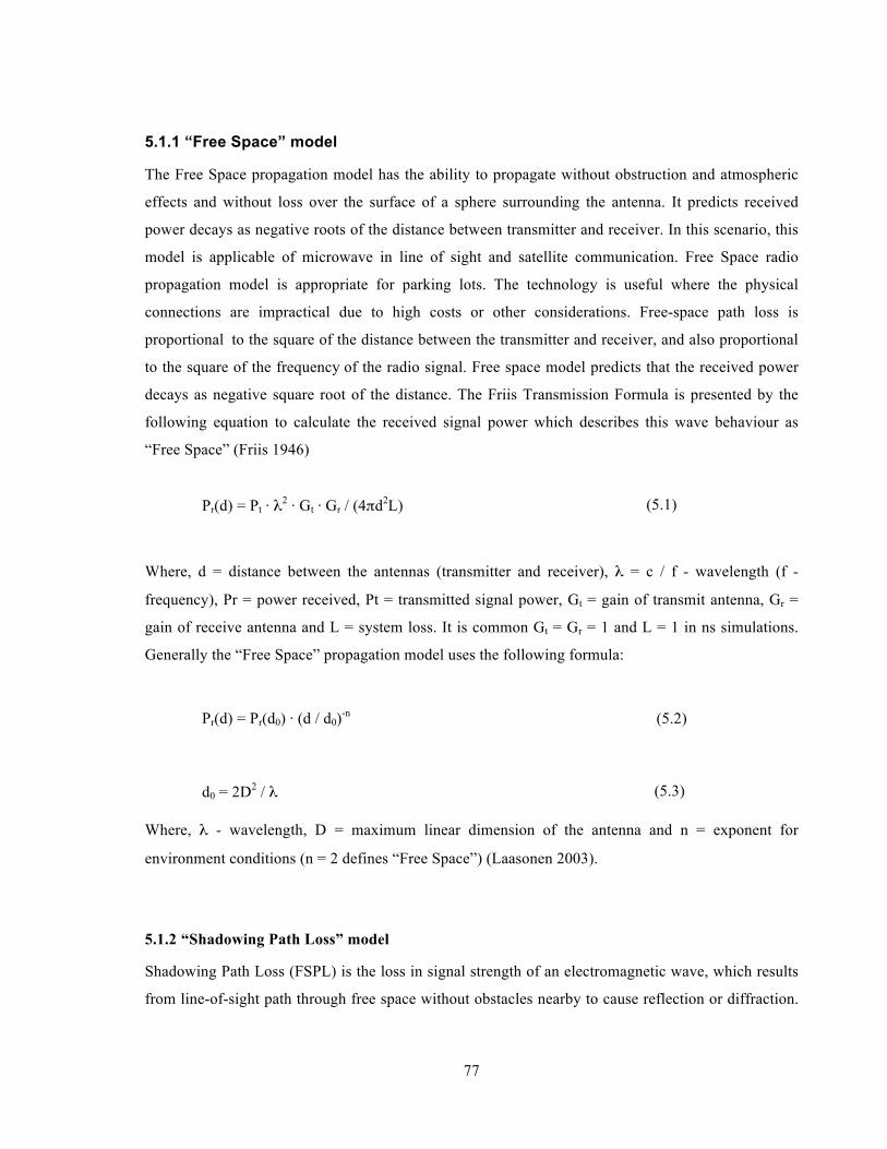
77
5.1.1 “Free Space” model
The Free Space propagation model has the ability to propagate without obstruction and atmospheric
effects and without loss over the surface of a sphere surrounding the antenna. It predicts received
power decays as negative roots of the distance between transmitter and receiver. In this scenario, this
model is applicable of microwave in line of sight and satellite communication. Free Space radio
propagation model is appropriate for parking lots. The technology is useful where the physical
connections are impractical due to high costs or other considerations. Free-space path loss is
proportional to the square of the distance between the transmitter and receiver, and also proportional
to the square of the frequency of the radio signal. Free space model predicts that the received power
decays as negative square root of the distance. The Friis Transmission Formula is presented by the
following equation to calculate the received signal power which describes this wave behaviour as
“Free Space” (Friis 1946)
Pr(d) = Pt · λ2 · Gt · Gr / (4πd2L) (5.1)
Where, d = distance between the antennas (transmitter and receiver), λ = c / f - wavelength (f -
frequency), Pr = power received, Pt = transmitted signal power, Gt = gain of transmit antenna, Gr =
gain of receive antenna and L = system loss. It is common Gt = Gr = 1 and L = 1 in ns simulations.
Generally the “Free Space” propagation model uses the following formula:
Pr(d) = Pr(d0) · (d / d0)-n (5.2)
d0 = 2D2 / λ (5.3)
Where, λ - wavelength, D = maximum linear dimension of the antenna and n = exponent for
environment conditions (n = 2 defines “Free Space”) (Laasonen 2003).
5.1.2 “Shadowing Path Loss” model
Shadowing Path Loss (FSPL) is the loss in signal strength of an electromagnetic wave, which results
from line-of-sight path through free space without obstacles nearby to cause reflection or diffraction.

78
FSPL is used in many areas for predicting radio signal strength which might be expected in radio
systems. While FSPL does not control most earthly circumstances because of object path and effects
from the ground, the FSPL model is very beneficial for simple thoughtful numerous real life radio
propagation situations and it can be approximately used for calculations for short distances or
numbers of areas where there are few obstructions The FSPL is rarely used separately but as part of
the Friis transmission equation, which contains the gain of antennas (Sommer, Joerer et al. 2012).
(5.4)
Where, λ - wavelength, d = distance between the antennas (transmitter and receiver), c = speed of
light in a vacuum and = the signal frequency.
5.1.3 “Egli” model
The Egli model is a terrain model for radio frequency propagation. Egli model calculations are used
to mathematically calculate propagation loss, which is the distance between transmitter and receiver.
The Egli model is simplified as "gently rolling terrain with average hill heights of approximately 50
feet (15 m)" (Roslee and Kwan 2010). The Egli model is mathematically expressed as:
(5.5)
Where, Pr = receive power, Pt= Transmit power, Gb= Gain the base station antenna, Gm=Gain of the mobile station antenna, hB= Height of the base station antenna, hM= Height of the mobile station antenna, d = Distance from base station antenna and f = Frequency of transmission.
5.1.4 “Hata” model
The Hata model creates an experimental mathematical link to define the graphical information
specified by Okumura. This model is mostly used for radio frequency propagation models for
predicting the behaviour of cellular transmissions in built up areas. This model includes the graphical
information from the Okumura model and improves it to understand the effects of reflection,
diffraction and scattering caused by city structures. The Hata model creates a number of

79
representative path losses for each urban, suburban and country environment (Nadir and Ahmad
2010).The Hata model is mathematically expressed below:
For urban areas,
(5.6)
For small or medium-size city
(5.7)
For larger cities,
(5.8)
Where, Lu= Path loss in urban areas, hB= Height of base station antenna, hM= Height of mobile
station antenna, f= Frequency of transmission, CH= Antenna height correction factor, d= Distance
between the base and mobile stations.
5.1.5 “COST 231” model
The European COST 231 recommended a model for indoor office propagation where attenuation
linearly produces the amount of walls traversed and the result of floors is non-linear. The COST 231
model covers modifications for urban, suburban and urban environments, which is proposed to extend
the Hata model. This model is limited to cases where the base station antenna is positioned higher
than nearby buildings (Dalela, Prasad et al. 2012). The COST 231 model is mathematically expressed
as:
((n+2)/(n+1)-0.46)
L = Lfs + 37 + 3.4 kw1 + 6.9 kw2 + 18.3 n
(5.9)
Where, L = attenuation, Lfs = free space loss and number of traversed floors, kw1 = number of light
internal walls, kw2 = number of concrete or brick internal walls

80
5.2 Model versus measurement: Comparative study
The following presents measured data, along with modeled data generated by the “Free Space”,
“Shadowing Path Loss”, “Egli”, “Hata” and “COST 231” models. The paths selected for this study
were chosen because they were considered to provide results illustrative of the models’ overall
performance features for short-range propagation paths. Estimated received signal power obtained
based on the corrected propagation models are more fitting to the measurement data. The measured
received signal power and that estimated using each of the corrected propagation models were
calculated using equations 5.1, 5.4, 5.5, 5.6, and 5.9 for “Free Space”, “Shadowing”, Egli, Hata and
“COST 231” models. The accumulated path losses for the 5 models are shown in Figures 5.1, 5.2, 5.3,
5.4, and 5.5, and all 5 models’ numeric results are shown in Appendix E. The result of received signal
strength vs. distance plot deploying the 5 models is as shown in the graph. After determining the path
loss of the practical measurements for each distance, the study was agreed on in order to create a
difference among the experimental and theoretical models values and the result. It is only theoretical
data and it may vary from the data obtained in real applications due to the environment or operating
circumstances though bigger loss at higher frequencies can be seen clearly.
Figure 5.1 shows (scenario 1) the comparison of path loss of different propagation models with
measured path loss results obtained for each propagation model are presented in the form of a plot. It
can be seen from the figure that the “Free Space” and “Hata” models have the lowest path losses
prediction -40.04 dBm to -75.46 dBm and -24.73 dBm to -104.24 dBm for 1m to 59m. The RSSI
value change follows a nearly similar pattern, which is RSSI drops gradually when the distance
increases. The “Free Space” model gave the highest prediction when it was -40.4 dBm to -73.11 dBm
in about 1m to 45m distance. Under non-LoS conditions “Free Space” and “Hata” models marginally
distorted the nature of the curve of the dependency of the received signal power from a distance, but
had a very good agreement with the level of the measurement data. As well it can be seen from the
figure that the “COST 231” “Egli”, and “Shadowing Path Loss” models had the highest path loss
prediction -77.04 dBm to 112.46 dBm, -40.04 dBm to -106.39 dBm and -33dBm to -68.5 dBm for 1m
to 59m. Under non-LoS conditions “COST 231”, “Egli” and “Shadowing Path Loss” models basically
do not work with the presented dependence of power received from a distance. That is something
which is unrealistic. Hence, its values can be ignored. However, based upon the measured and
models’ results presented in this study, it is clear that the “Hata” and “Free Space” models are a closer
match and have a very good agreement with the level of the measurement data. Other models

81
overestimated the path loss for the indoor propagation environment. According to these results for
scenario 1, the “Free Space” is recommended for the evaluation of comparable partition inspiration on
the signal propagation under NLOS conditions. The “Free Space” model, which is capable of
providing path loss, estimates significantly closer to actual values than other models.
Figure 5.1: RSSI versus distance for NLOS condition: Comparison of measurement and five models
Figure 5.2 shows (scenario 2) the comparison of path loss of different propagation models with
measured path loss results obtained for each propagation models presented in the form of a plot . It
can be seen from the figure that the “Egli” model has the lowest path loss prediction –59.64 dBm to –
85.24 dBm for 4 m to 17.46 m. The RSSI value change follows a nearly similar pattern, which is
RSSI drops gradually when the distance increases. The “Hata” model gave the highest prediction.
Under non-LoS conditions the “Hata” model marginally distorted the nature of the curve of the
dependency of the received signal power from a distance, but had a good agreement with the level of
the measurement data. As well it can be seen from the figure that the “Shadowing Path Loss”, “Free
-‐120
-‐110
-‐100
-‐90
-‐80
-‐70
-‐60
-‐50
-‐40
-‐30
-‐20
1 5 9 13 17 21 25 34 38 48 55 59
RSSi (dBm
)
Distance (m)
Measurement Shadowing Path Loss Free Space
Egli Hata COST231

82
Space”, “Egli”, and “COST 231” models have the highest path loss prediction -45.1 dBm to -57.4
dBm, -52.08 dBm to -64.88 dBm and -59.64 dBm to -85.24 dBm, and -134.94 dBm to -147.78 dBm
for 4m to 17.46m. Under non-LoS conditions “Shadowing Path Loss”, “Free Space”, “Egli”, and
“COST 231” models, did not work with basically the presented dependence of power received from a
distance. That is something which is unrealistic. Hence, its values can be ignored. However, based
upon the measured and models results presented in this study, it is clear that the “Hata” model is a
closer match and has a very good agreement with the level of the measurement data. Other models
overestimate the path loss for the indoor propagation environment. According to these results for
scenario 2, the “Hata” model provides maximum accuracy and flexibility with signal propagation
modes and is recommended for the evaluation of comparable partition inspiration on the signal
propagation under NLOS conditions. The “Hata” model, which is capable of providing path loss,
estimates significantly closer to actual values than other models.
Figure 5.2: RSSI versus distance for NLOS condition: Comparison of measurement and five models
-‐170
-‐150
-‐130
-‐110
-‐90
-‐70
-‐50
-‐30
RSSI (dBm
)
Distance (m)
Measurement Shadowing Path Loss Free Space
Egli Hata COST231

83
Figure 5.3 shows (scenario 3) the comparison of path loss of different propagation models with
measured path loss results obtained for each propagation model presented in the form of a plot. It can
be seen from the figure that the “Egli” model has the lowest path loss prediction, –71.64 dBm to -
74.54 dBm for 8m to 9.43m. The RSSI value change follows a nearly similar pattern, which is RSSI
drops gradually when the distance increases. The “Egli” model gave the highest prediction when it
was -71.64 dBm in about 8m distance. Under non-LoS conditions the “Egli” model marginally
distorted the nature of the curve of the dependency of the received signal power from a distance, but
had a very good agreement with the level of the measurement data. As well it can be seen from the
figure that the “Shadowing Path Loss”, “Free Space”, “Hata”, and “COST 231” models have the
highest path loss prediction –51.1 dBm to 52.5 dBm, --58.1 dBm to -59.53 dBm, -65.27 dBm to -
68.28 dBm and -156.23 dBm to -157.65 dBm for 8m to 9.43m. Under non-LoS conditions the
“Shadowing Path Loss”, “Free Space”, “Hata”, and “COST 231” models, basically do not work with
the presented dependence of power received from a distance. That is something which is unrealistic.
Hence, its values can be ignored. However, based upon the measured and models results presented in
this study, it is clear that the “Egli” model is a closer match and has a very good agreement with the
level of the measurement data. Other models are overestimate the path loss for the indoor propagation
environment. According to these results for scenario 3, the “Egli” model provides maximum accuracy
and flexibility with signal propagation modes and is recommended for the evaluation of comparable
partition inspiration on the signal propagation under NLOS conditions. The “Egli” model, is capable
of providing path loss estimates significantly closer to actual values than other models.

84
Figure 5.3: RSSI versus distance for NLOS condition: Comparison of measurement and five models
Figure 5.4 shows (scenario 5) the comparison of path loss of different propagation models with
measured path loss results obtained for each propagation models are presented in the form of a plot .
It can be seen from the figure that the “Free Space” and “Shadowing Path Loss” models have the
lowest path losses prediction -60.87 dBm to -76.69 dBm and -53.9 dBm to -69.7 dBm for 11m to
68m. The RSSI value change follows a nearly similar pattern, which is RSSI drops gradually when
the distance increases. The “Free Space” model gave the highest prediction when it was -60.87 dBm
to -72.3 dBm in about 11m to 41m distance, as well, the “Shadowing Path Loss” model gave close
prediction when it was -53.9 dBm to -57.1 dBm in about 11m to 16m distance. Under non-LoS
conditions the “Free Space” and “Shadowing Path Loss” models marginally distorted the nature of the
curve of the dependency of the received signal power from a distance, but had a very good agreement
with the level of the measurement data. As well it can be seen from the figure that “Egli”, “Hata”,
and “COST 231” models had the highest path loss prediction -77.21 dBm to 108.86 dBm, -71.48 dBm
to -107.01 dBm and -125.47 dBm to -140.76 dBm for 11m to 68m. Under non-LoS conditions the
“Egli”, “Hata”, and “COST 231” models, basically do not work with the presented dependence of
-‐180
-‐160
-‐140
-‐120
-‐100
-‐80
-‐60
-‐40
8 8.06 8.24 8.54 8.94 9.43
RSSI (dBm
)
Distance (m)
Measurement Shadowing Path Loss Free Space
Egli Hata COST231

85
power received from a distance. That is something which is unrealistic. Hence, its values can be
ignored. However, based upon the measured and models results presented in this study, it is clear that
the “Shadowing Path Loss” and “Free Space” models are a closer match and have a very good
agreement with the level of the measurement data. Other models overestimate the path loss for the
indoor propagation environment. According to these results for the scenario 5, the “Free Space”
model provides maximum accuracy and flexibility with signal propagation modes and is
recommended for the evaluation of comparable partition inspiration on the signal propagation under
NLOS conditions. The “Free Space” model, is capable of providing path loss estimates significantly
closer to actual values than others models.
Figure 5.4: RSSI versus distance for NLOS condition: Comparison of measurement and five models
In our comparisons of different indoor propagation models on the basis of theoretical path loss with
field measurement data it was revealed during the comparative study of different models along with
-‐150
-‐140
-‐130
-‐120
-‐110
-‐100
-‐90
-‐80
-‐70
-‐60
-‐50
11 15 19 23 27 31 35 39 43 47 51 55 59 63 67
RSSI (dBm
)
Distance (m)
Measurement Shadowing Path Loss Free Space
Egli Hata COST231

86
interpolated measured field data values that out of the different models studied only five specific
models closely approximate the actual measurement characteristics, namely: “Free Space”,
“Shadowing Path Loss”, “Egli”, “Hata” and “COST 231” models.
All other models showed huge deviation from the measured field data value, which clearly indicates
inefficiency of all other models to be deployed for network planning in this region; however, it can be
seen from Figures 5.1 and 5.4, that the received signal power estimated using the corrected “Free
Space” propagation model shows a good fit with measured received signal power for the required
distance.
5.3 Summary
This chapter presented radio propagation models, which are “Free Space”, “Shadowing Path Loss”,
“Egli”, “Hata” and “COST 231” models that can be used to predict signal strength of planning
VANETs based on measurement results. By conducting all measurements, all possible procedures to
adjust or modify existing models can be chosen. It is clear that the received signal power in scenario
1, “Free Space” model and Hata model are better than other models. In scenario 2, the Egli model is
closer and has very good agreement with the level of measurement data. In scenario 3, the Egli model
is a bit closer than other models. In scenario 5, the “Free Space” propagation model is closer and has
a very good agreement with the level of the measurement data. Implications and recommendations for
deployment of VANET in a large shopping mall are presented in Chapter 6,

87
Chapter 6
Implications and Recommendations for System Deployment
Chapter 5 discussed the comparative study of models versus measurement. This chapter presents
implications which provide significantly well-organized choosing of appropriate positions in similar
environments in section 6.1, and section 6.2 discusses recommendations for VANET development
such as wireless access points, smart antenna for wireless, indoor radio WLAN performance, ad hoc
localized position systems, cross-layer design of ad hoc networks and trust and reputation
management framework.
6.1 Implications
By conducting numerous preliminary field-trial measurements in the West City Auckland shopping
mall parking lot and propagation models, we expanded an understanding into the radio propagation
performance of an IEEE 802.11n network. The initial measurements support us to understand IEEE
802.11n configuration and practical deployment as well provide reference for our data used for
analysis. The features of the wireless adapter would differ with special models and vendors.
Our study findings stated the contribution of a particular purpose, which is to provide significant
implications and be well-organized in choosing appropriate positions in a similar environment.
Firstly, our findings, as described in this paper, might be beneficial for administrators to deploy
informed assessments about the expansion of IEEE 802.11n in locations similar to the West City
Auckland shopping mall parking buildings. Secondly, this study demonstrates, by measurement, the
straight influence West City Auckland shopping mall parking lot separation and RSS on system
performance, which is genuine hardware to measure performance, escaped the difficulty of theoretical

88
modeling of radio signal propagation and system implementation. Thirdly, our study measurement
results specify that RSS was not sufficient to represent the actual performance of WLANs. So a wide
measurement study is primarily required to develop further accurate results before any practical
VANET as table 6.1 shows. Wireless access in vehicular environment forces a set of the latest
requirements on the communications system that controlled to the indication of the WAVE functional
mode and of the WAVE BSS in IEEE 802.11p, which theatrically decreases the connection setup
transparency and suits vehicular safety applications well.
Table 6.1: VANET features and implications
Features Implications
Wireless Access Point Strength range in VANET environment
Wireless Communication and radio signal propagation
Restricted bandwidth and error-prone wireless communication.
High Mobility Short communication periods
Beaconing Further network capacity, but protocols can advantage from information exchanged by this basic service.
Dissemination delay Safety applications require instant relaying of information
Delay Constraints Any messages must need to be broadcast instantly, without introducing any delay.
Fourthly, video and audio conferencing in inter-vehicle communications in VANET need to be
sophisticated implications because faster data transfer needs longer connection lifetime. VANET
vehicles (nodes) are expected to be equipped with calculations encryption and others vehicles
positions, vehicle track location with GPS receiver enabling, communication devices to propagate
/receive information, set a sensors to report such as weather conditions, safety for crashes require to
deliver of emergency warning messages, vehicle statistics etc., dedicated and secured memory to
strong log files. Multi-hop data dissemination without aggregation concept every vehicle would need
to broadcast for position and speed information which in turn disseminates to support approaching
vehicles to avoid traffic jams. Finally, identifying misbehavior in VANET’s significant issues in
extensive range of implications with safety related and congestion avoidance applications.

89
6.2 Recommendations for system Deployment
Based on the study in the previous section, we have designed a parking environment with Vehicular
Ad Hoc Networks as shown in Figure 6.1. A wireless access point is a device that allows wireless
devices to connect to a wired network using Wi Fi. Internet-enabled nodes access points have a robust
benefit, with the possibility of having numerous access points connected by a WLAN.
Figure 6.1: Deployment Scenario - a VANET in the parking lot

90
Recommendations for system deployment
The following are guidelines to be recommended for system development in the future:
1. Analyzing inter-floor signal propagation. Because every building is different it is a good idea to
do some testing and determine how much the floors actually attenuate the radio signal. The
following are steps that should be completed when analyzing inter-floor signal propagation:
Identify Primary Requirements:
Ø Type of facility (Access the construction of the facility which includes ceiling
tiles, wood, concrete, steel etc.)
Ø Type of client devices
Ø Industry vertical
Identify Customer Facility Requirements
Ø Single-floor
Ø Multi-floor
Ø Campus (indoor and outdoor)
Identify Requirements for Type of Client Devices
Ø Minimum Received Signal Strength Indicator
Ø Minimum Signal-to-Noise Ratio
Ø Delay and Jitter tolerance
Ø Maximum transmit (Tx) power
Wireless access points are exceptional for the purpose of communication devices on wireless local
area networks, which are a central transmitter and receiver of the wireless radio signal. Each access
point has its own radio range for communication with a network adapter, which is 20m to more than
300m depending on product specification and antenna and operation environment. Multiple access
procedure affects share the wireless network connection to end-user because the transmitter-to-
receiver frequency spacing has to be carefully controlled in order to avoid unaccountably complex
filters. In an environment multiple access technology concept is the best possible way for combing,
instance, multiple coverage with high bandwidth WLAN hot spots. Panko (2002) presented 15%
radio signal overlaps when placing multiples. Vehicular Ad Hoc Network extension is one of the
recommendations. The access network operates in the infrastructure mode and can be retrieved by

91
normal users with no specific software. The following are steps which should be completed for
analyzing inter-floor signal propagation:
Ø Measure inter-floor signal propagation
Ø Characterise the inter-floor propagation
Ø Determine access point placement
Ø Avoid placing access points near structures
Ø Use power to deploy wireless access points
Ø Avoid overlapping DHCP scopes
Ø Use meaningful SSID
2. Apply smart antenna technology, which consists of multiple antenna elements for wireless
environments to systems which can provide better performance for radio propagation signals
where wireless communications are limited in performance and capacity. Multiple transmit and
multiple receive antennas can provide multiple independent channels to increase data rate smart
antennas which can significantly improve the performance of wireless systems. Fixed antenna can
increase gain for better coverage and can be used for downlink or uplink. The researchers’
measurement with 4 antennas at access point in IEEE 802.11a for real-time implementation
where the result shows 6 db gain rise for 40% better range and process with an equivalent power
interferer with possible to more than double with rapid fading and provides up to 216 Mpbs in 20
MHz bandwidth (Winters 1998). In indoor environments propagated electromagnetic signals can
undergo three main physical modes, which are reflection, diffraction, and scattering. Moreover, a
Toroidial Helical Antenna provides up to 300 percent performance improvement because antenna
fading is not an issue and nearly isotropic direction. The radio spectrum is a limited resource and
solutions need to maximize that can get better radio signal. Installing metal shielding can be
effective.
Table 6.2: Smart Antenna technology
High Efficiency Very Low Cost Compact Size Frequency range from 450MHz to 6GHz
One antenna replaces all others Size reductions up to 75x
Wide bandwidth One antenna replaces all others Flexible High port isolation Flexible implementation in foil
or copper Occupies very little space
3. Co-channel users on the similar channel are factually protected from another decreasing the
chance of interface. The authors were using RSSI readings to evolution the channel simulation

92
and to recreate interface. Moreover, channel modeling could decrease the received signal by
obstructing LOS signal propagation (Boban, Vinhoza et al. 2011).
4. Assigning Radio Frequency (RF) channels and wireless network deployment, should be an
alternative to the use of RF channels in a manner that minimizes inter-access-point interference.
The weakness of non-overlapping channels in the 2.4GHz band makes it extremely problematic
and sometimes difficult to sustain inter-access-point interference down to satisfactory levels in
multi-floor buildings, particularly when supporting high-capacity voice systems. Consequently, it
is advisable to migrate to 5GHz 802.11n. The 5GHz spectrum contains a comparatively big
number of non-overlapping channels, which significantly reduces channel reuse problems and
improves the performance of the network.
5. Wi-Fi extenders simply piggyback on existing Wi-Fi connections and rebroadcast and it is a good
way to extend coverage. Wi-Fi extenders are placed in between a base router or access point and
users that are not close enough to receive acceptable services or one that is on the other side of a
barrier. They connect wirelessly to the router or access points, pick up the signal and retransmit it
to the users.
6.3 Summary
This chapter discussed implications and recommended solutions provided to show that these proposed
solutions actually work and can improve network performance in future VANET development. The
performances can be developed to deploy a number of access points in an indoor parking
environment. In Chapter 7, will be discussed research conclusions and possibilities for future
research.

93
Chapter 7
Conclusions and Future resarch Chapter 6 outlined system implications and recommendations for VANET deployment in a large
shopping mall. In this chapter, section 7.1 discusses the summary and conclusions for each chapter.
Section 7.2 presents for future research emphasis on the investigation of the impact of security
mechanisms on Wi-Fi throughput, which would provide suggestions for significant vision vehicle
safety, and information services into choosing security mechanisms for VANET deployment.
7.1 Summary and Conclusions
The main objective of this thesis was to provide for network planners to implement an IEEE 802.11-
based VANET in the parking lot of a large shopping mall and a best-fit propagation model in
measurement scenario. This study also illustrated a field trial measurement approach in IEEE 802.11n
to implement the testing environment, collect data and analyze data with propagation models to
achieve an accurate and realistic RSSI and transmission time of WLAN in the obstructed West City
Auckland shopping mall parking lot environment. Recently researchers have proposed studies about
VANETs environments. However, very few studies have proposed for network planners to implement
an IEEE 802.11-based VANET in a large parking shopping mall. A deeper understanding of the
impact RSSI in VANET’s performance has been obtained by conducting various measurements and
simulation experiments in this study. The preliminary results gave a clear indication of which
VANET’s parking lot scenarios perform best in a given situation. These results not only help by
doing a virtual analysis but also give an insight into the variables that are VANET’s performances and
a better judgment of which IEEE 802.11-based VANET is to be used in a similar situation in the
future.
Chapter 1 introduced the basis of this research, outlined the motives, aims and organizational
structure of this research.

94
Chapter 2, reviewed vehicular ad-hoc communications with VANET applications and
classifications, VANET issues and challenges, which provided us with a better understanding of
VANET implications. Moreover VANET provides massive chances and opportunities in online
vehicle entertainments such as through the local ad hoc networks sharing pictures, video, files,
gaming and chatting. In order to use 802.11 standards technology, a fundamental understanding is
required for designing, deploying and testing for best performance. However IEEE 802.11n have been
designed for better signal strength and data rates for VANET communications. This kind of network
relies on the use of short range networks (about 100 meters) with IEEE 802.11 for vehicle
communication and providing bandwidth in the range of MBPS. Radio propagation was also
addressed in this study, which can affect RSSI and throughput on the wireless network. In simulation
environments, VANETs can appropriately model how vehicles move in a proper environment of ad
hoc communication performance. Models that apply different types of attenuation features on the
comparative heading nodes and positions proposed a suitable method to resolve these issues. A good
understanding of how VANETs behave, the influential factors and performance issues that stimulate
or cause a drawback is required to identify areas of improvement in VANETs deployment. The flow
charts and contributions by researchers helped to isolate the gap where improvement is required.
In Chapter 3, the detailed experimental design and planning of propagation in the West City
Auckland shopping mall parking lot environment are presented. Table 3.1 in Chapter 3 presented
details of Wi-Fi-Based Vehicular Ad Hoc Networks using field trial measurement scenarios. As well,
tables 3.2 and 3.3 in Chapter 3 describe clearly the OPNET parameters used in the configuration of
the experiments and the numbers of experiments conducted in a particular scenario.
Chapter 4 generated experimental results on the performance of VANETs. The performance
measurement of a VANET is considered by the four performance metrics RSSI, transmission time,
sent data rate and received data rate. The results are classified into 5 scenarios for measurement. In
scenario 1 and 5, we found RSSI gave best performance till 31m, which is -74 dBm. However the rest
of the scenarios got poor signal coverage due to the concrete roof and wall barriers. Finally, the
OPNET based scenario consisted of six experiments (time average delay, throughput, traffic sent,
traffic received, download file size and download response time) according to two applications FTP
and P2P, and network sizes 2, 5, 10, 20, 30, 40 and 50 nodes. OPNET simulations represent the end-
to-end delay of all the data packets, collected separately for each 802.11n and successfully received
by all the 802.11n capable WLAN MACs in the network and forwarded to a higher layer. Network
mean packet delays are 1.72, 2.89, 3.06, 2.91, 3.08, 3.2 and 2.9 ms for N = 2, 5, 10, 20, 30, 40 and 50,

95
respectively, and network mean throughput are 5.6, 10.3, 17.5, 32.8, 55.63, 70.01 and 69.9 kbps for N
= 2, 5, 10, 20, 30, 40 and 50, respectively.
Chapter 5, presented radio propagation models, which are “Free space”, “Shadowing Path Loss”,
“Egli”, “Hata” and “COST 231” models that can be used to predict the signal strength of planning
VANETs based on measurement results. It is clear from the received signal power in scenario 1, the
“Free Space” model and Hata model is better than other models. In scenario 2, the Egli model was
closer and has very good agreement with level of measurement data. In scenario 3, the Egli model
was bit closer than any other model. In scenario 5, the “Free Space” propagation model was closer
and had a very good agreement with the level of the measurement data because there was no obstacle
or reflected area effect between transmitter and receiver.
The models can be used in all kinds of indoor radio wave propagation to approximate signal
attenuation for signal and multi floor wireless links using such building nature. We consider that the
outcomes of our measurement result could save researchers time through discarding unnecessary
issues when accomplishing simulations for VANET-related research or implementing VANET in any
indoor parking environment. This approach can be a beneficial tool to help in approximating the
signal power any place in the building, and wireless indoor communication coverage so this approach
could be useful for all types of VANET indoor radio communications environments. The data
measured in the simulation network illustrates the outcome of measurement conducted in real
VANET scenarios. The performances can be developed to deploy a number of access points in indoor
parking environments. The recommended solution might provide simulations to show that these
proposed solutions actually work and can improve network performance in future VANET
development.
7.2 Future Reserch
In this thesis significant numbers of issues arise which can affect radio propagation signal power. This
section outlines a number of possible extensions to this research that could help further understanding
of the problem.
• We only considered an ad hoc network in the study. An infrastructure network using wireless
access points to carry out the field trial measurements would be a logical extension to the
work presented in this thesis. Wireless Access Point especially supports public hotspots Wi

96
Fi network in a large building where space is required for wireless coverage. The work can
be further extended by considering vehicle mobility
• Deploy some sensor networks around the parking lot to collect data regarding moving
vehicles (cars) and then repeat field trial measurements by considering both ad hoc and
infrastructure network. Sensor networks agree a system to be extended from one with simple
functions to one that can receive and act on data about the environment it operates in.

97
Appendix A: Wi-Fi around West City shopping mall parking lot
Table A1: Level 1 in West city shopping mall parking lot
Table A2: Level 2 West city shopping mall parking lot
SSID RSSI (dBm) Channel
Spark Westcity -78 7
Guest WaiFi -87 11
Colubris Networks -73 3
ANZ WTB Hotspot -86 8
ANZ Public Hotspot -88 8
ASB Customer WiFi -87 13
SmartServiceWestcity -87 5
Koffee Bar Free Wifi -79 11
SSID RSSI (dBm) Channel
Spark Westcity -80 7
Shing -78 11
Colubris Network -86 3
Koffee Bar Free Wifi -75 11
DSE -88 2
Smart Service Westcity -83 5
DSE-Internal -82 4
Smart Service Westcity -85 5
ASB Customer WiFi -83 13
SS -86 11
DSE -87 4
Smart Service Westcity -85 5
Magstar -87 9
No1ShoesWiFi -84 6
TNZ-4279 -87 13
Spark-BPTA5W -86 8
TPM Training -87 11
ANZ Public Hotspot -87 8
ANZ WTR Hotspot -86 8

98
SmartServiceWestcity -87 5
SS -86 11
Shing -74 11
No1ShoesWiFi -84 6
Magstar -85 9
Spark- BPTA5W -87 8
CE Only -85 11
TPM Training -89 11
Test -87 11
SmartServiceWestcity -85 5
DSE -90 2
DSE-Internal -84 4
TNZ-4279 -87 13
DSE -84 4
Table A3: Level 3 West city shopping mall parking lot
SSID RSSI (dBm) Channel
Staff WaiFi -86 11
Thomson2959DF -67 16
Staff WaiFi -83 6
Test -83 11
Guest WaiFi -82 11
Koffee Bar Free WiFi -79 11
TPM Training -84 11
HP-Print-24-Officejet -87 1
Shing -80 11
Tomizone@Westfield -87 1
WiFi2 -86 1
Guest WaiFi -86 6
Test -84 6
No1ShoesWiFi -84 6
CE Onlt -86 6
CE Only -83 11
WiFi1 -87 1
Tomizone@Westfield -87 1

99
Table A4: Level 4 West city shopping mall parking lot
SSID RSSI (dBm) Channel
Staff Wifi -81 11
Thomoson2959DF -74 6
Staff WaiFi -82 6
Test -78 11
Guest WaiFi -77 11
Koffee Bar Free WiFi -77 11
TPM Training -77 11
HP-Print-24Officejet -85 1
Shing -77 11
Tomizone@Westfield -87 1
Wifi2 -84 1
GuestWifi -81 6
Test -83 6
No1ShoesWifi -87 6
CE Only -80 6
CE Only -73 11
WiFi1 -88 1
Tomizone@Westfield -90 1
Guest WaiFi -88 1
Ovl-chwap1 -88 9
WiFi1 -86 1
WiFi2 -87 1
Bbw -88 7
Vodafone37CB -87 11
TNCAPD24173 -88 6
Guest WaiFi 80 6
Fhlwpa2ccmp -87 1
StaffWiFi -86 1
StaffWiFi -80 6
Test -86 1
CR Only -82 6
DSE-Internal -85 4
CR Only -88 1
DSE -86 4

100
Test -82 6
Table A5: Edsel Street in West city shopping mall parking lot
SSID RSSI (dBm) Channel
Staff WaiFi -67 6
Test -72 6
CE Only -68 6
Koffee Bar Free WiFi -87 11
Staff WaiFi -74 11
Guest WaiFi -74 11
CE Only -74 11
Megatel-00286 -83 1
No1ShoesWiFi -79 6
Test -76 6
Test -75 11
shing -85 11
TPM Training -73 11
CE Only -80 1
ASB Customer WiFi -84 13
Dlink -84 11
Hp-Print-24-Officejet -82 1
Guest WaiFi -71 6
Staff WaiFi -85 1
AndroidAP -84 1
WTDEMO -83 16
Test -86 1
CE Only -80 6
VodafoneX5WU -78 1
BBw -88 7
Unknown -86 1
Staff WaiFi -84 6
Guest WaiFi -85 1

101
Lighting Direct -76 1
Guest WaiFi -79 6
VodafoneQ58F -88 1
Telecom-0482 -88 1
CE Only -87 11
TNZ-6060 -85 8
Elsha George -75 1
Net Com wireless -88 5

102
Appendix B: Preliminary Field trials results Table B1: Measurement al results Scenario 1 (802.11n) Distance
(m) RSSI
(dBm) Data Rate
(Bytes /sec) Transmission time (µs)
Data Rate (Bytes / sec)
Transmission time (ms)
File size 71 bytes File size 1.05 MB
1 -45 108 1.44 162454 2.167
2 -45 229 3.053 158988 2.12
3 -49 176 2.347 159182 2.123
4 -51 178 2.373 161420 2.152
5 -51 225 3 161994 2.16
6 -53 152 2.027 158925 2.119
7 -66 286 3.813 163001 2.173
8 -59 123 1.64 159182 2.123
9 -61 214 2.853 158564 2.115
10 -64 240 3.2 158981 2.12
11 -63 272 3.627 160876 2.145
12 -60 168 2.24 158786 2.117
13 -67 138 1.84 159548 2.127
14 -61 158 2.107 160138 2.135
15 -66 281 3.747 158958 2.12
16 -61 204 2.72 162151 2.163
17 -64 585 7.8 162766 2.171
18 -65 199 2.653 159690 2.129
19 -65 216 2.88 160674 2.143
20 -71 243 3.24 162340 2.164
21 -71 183 2.44 159845 2.131
22 -64 254 3.387 159536 2.127
23 -74 349 4.653 163859 2.185
24 -74 168 2.24 159880 2.132
25 -73 238 3.173 159913 2.132
31 -74 601 8.013 171138 2.281
32 -83 545 7.267 179631 2.395
33 -90 422 5.627 165105 2.201
34 -74 237 3.16 171138 2.281
35 -83 315 4.2 179631 2.395

103
36 -71 311 4.147 178751 2.384
37 -83 269 3.587
38 -74 202 2.693
44 -82 212 2.827
45 -74 370 4.933
46 -90 218 2.907
48 -83 267 3.56
49 -90 360 4.8
50 -91 487 6.493
52 -90 654 8.6
55 -83 349 4.653
56 -83 601 8.013
57 -83 1120 14.93
Table B2: Measurement results Scenario 2 (802.11n) Distance
(m) RSSI
(dBM) Data Rate
(Bytes / sec) Transmission
time (µs) Data Rate
(Bytes / sec) Transmission
time (ms)
File size 71 bytes File size 1.05 MB
4 -73 139 1.853 122924 1.639 4.12 -74 141 1.88 122804 1.637
4.47 -90 132 1.76 125105 1.668 5 -91 615 8.2 125322 1.671 5.65 -82 118 1.573 122976 1.64 6.4 -83 100 1.333 124388 1.659 7.21 -82 828 11.04 123349 1.644 8.06 -82 112 1.493 124573 1.661 8.94 -83 218 2.907 123641 1.648 9.84 -83 1935 25.8 10.77 -90 2165 28.87 11.7 -83 725 9.667 12.65 -90 2745 36.6 13.6 -90 2237 29.83 14.56 -91 2175 29 15.52 -91 2835 37.8 16.49 -91 2856 38.08 17.46 -90 2165 28.87

104
Table B3: Measurement results Scenario 3 (802.11n) Distance
(m) RSSI
(dBm) Transmission
time (µs) Data Rate
(Bytes / sec) Data Rate
(Bytes / sec) Transmission
time (ms))
File size 71 bytes File size 1.05 MB
8 -74 3.36 252 125619 1.691 8.06 -83 1.48 111 126837 1.691 8.24 -91 3.52 264 8.54 -91 9.613 721
Table B4: Measurement results Scenario 4 (802.11n) Distance
(m) RSSI
(dBm) Transmission
time (µs) Data Rate
(Bytes / sec) Data Rate
(Bytes / sec) Transmission
time (ms)
File size 71 bytes File size 1.05 MB 12 -0 0 0 0 0 12.04 0 0 0 0 0 12.17 0 0 0 0 0
Table B5: Measurement results Scenario 5 (802.11n) Distance
(m) RSSI
(dBm) Data Rate
(Bytes / sec) Transmission
time (µs) Data Rate
(Bytes / sec) Transmission
time (ms) File size 71 bytes File size 1.05 MB
11 -55 275 3.667 163876 2.185 12 -58 264 3.52 159786 2.131
13 -60 276 3.68 159948 2.132 14 -59 368 4.907 163568 2.181
15 -62 310 4.133 158858 2.119 16 -58 292 3.893 169851 2.265
17 -64 423 5.64 162706 2.169 18 -70 313 4.173 158790 2.117
19 -65 316 4.213 164874 2.199 20 -69 462 6.16 162340 2.164 21 -71 296 3.947 159885 2.132 22 -74 319 4.253 158536 2.113 23 -70 364 4.853 166859 2.225
24 -73 370 4.933 159680 2.129 25 -69 438 5.84 159726 2.13 26 -68 412 5.493 160033 2.133 27 -70 443 5.907 166072 2.215 28 -73 456 6.08 159720 2.129

105
29 -73 471 6.28 163929 2.185 30 -72 534 7.12 177288 2.185 31 -71 601 8.013 182045 2.427 32 -80 640 8.533 176016 2.347 33 -74 422 5.627 165405 2.205
34 -81 437 5.827 155181 2.069 35 -79 315 4.2 158751 2.117
36 -75 390 5.2 178901 2.385 37 -78 469 6.253 189721 2.529 38 -74 475 4.027 185312 2.471
39 -71 398 5.307 179260 2.391 40 -80 487 6.493 185371 2.472 41 -74 431 5.747 184276 2.457 42 -81 461 6.147 189572 2.528 43 -79 495 6.6 190254 2.537 44 -84 468 6.24 185129 2.468 45 -70 490 6.533 172316 2.297
46 -89 432 5.76 179321 2.391 48 -81 418 5.573 196541 2.62 49 -89 439 5.853 189654 2.529 50 -90 613 8.173 196521 2.62 51 -90 646 8.613
52 -89 413 5.507 53 -88 517 6.893 54 -78 556 7.413
55 -87 527 4.36 56 -83 518 6.907 57 -85 1125 15
58 -90 532 7.093 59 -92 467 6.227 60 -90 1029 13.72 61 -92 612 8.16 62 -89 859 11.45 63 -90 587 7.827 64 -92 864 11.52 65 -90 601 8.013 66 -89 632 8.427 67 -91 979 13.05 68 -92 1355 18.07

106
Appendix C: OPNET Simulations Configurations
Figure C1: Application configuration
Figure C2: Profile Configuration

107
Figure C3: WLAN configuration
Figure C4: Simulation result browser

108
Appendix D: OPNET-based Simulation Scenario Results
Table D1: Peer-to-Peer File sharing packet delay (ms)
2 Nodes 5 Nodes 10 Nodes 20 Nodes 30 Nodes 40 Nodes 50 Nodes 1.72 2.89 3.062 2.91 3.08 3.28 2.92
Table D2: Peer-to-Peer File sharing Throughput (kbps)
2 Nodes 5 Nodes 10 Nodes 20 Nodes 30 Nodes 40 Nodes 50 Nodes
5.63 10.35 17.54 32.81 55.63 70.01 69.96
Table D3: Peer-to-Peer File sharing traffic received (kbps)
2 Nodes 5 Nodes 10 Nodes 20 Nodes 30 Nodes 40 Nodes 50 Nodes Low Traffic 0.67 1.22 1.74 3.55 5.82 6.99 9.23 High Traffic 41.09 71.34 168.97 356.29 525.00 611.82 618.36
Table D4: Peer-to-Peer File sharing traffic sent (kbps)
2 Nodes 5 Nodes 10 Nodes 20 Nodes 30 Nodes 40 Nodes 50 Nodes Low Traffic 0.67 1.22941 1.74 3.55 5.82 6.99 9.23 High Traffic 41.09 71.34 168.97 367.03 580.39 750.28 3195.584
Table D5: Peer-to-Peer File download file size (mbps)
2 Nodes 5 Nodes 10 Nodes 20 Nodes 30 Nodes 40 Nodes 50 Nodes Low Traffic 0.06 0.05 0.053 0.06 0.05 0.04 0.05 High Traffic 6.16 4.13 5.17 5.66 4.83 4.35 4.61
Table D6: Peer-to-Peer File download response time (sec)
2 Nodes 5 Nodes 10 Nodes 20 Nodes 30 Nodes 40 Nodes 50 Nodes Low 1.26 0.10 0.27 0.23 0.60 0.22 0.11 High 56.84 36.35 26.80 43.90 60.24 71.34 53.83

109
Table D7: Ftp download response time (sec)
2 Nodes 5 Nodes 10 Nodes 20 Nodes 30 Nodes 40 Nodes 50 Nodes Low load 0.13 0.01 0.08 0.12 0.10 0.11 0.08 Medium load
0.0098 0.0095 0.0098 0.0099 0.0097 0.0099 0.0099
High Load 0.072 1.63 1.61 0.80 1.41 0.83 0.62
Table D8: Ftp upload response time (sec)
2 Nodes 5 Nodes 10 Nodes 20 Nodes 30 Nodes 40 Nodes 50 Nodes Low load 0.08 0.05 0.05 0.07 0.11 0.13 0.07 Medium Load
0.12 0.017 0.13 0.12 0.09 0.10 0.12
High load 3.45 1.02 1.67 0.75 0.84 0.86 0.90
Table D9: Ftp traffic received (kbps)
2 Nodes 5 10 Nodes 20 Nodes 30 Nodes 40 Nodes 50 Nodes Low load 0.01 0.02 0.05 0.10 0.16 0.22 0.26 Medium Load
0.09 0.09 0.25 0.53 0.72 1.03 1.31
High load 0.85 1.36 3.23 5.78 8.67 14.45 13.94
Table D10: Ftp traffic sent (kbps)
2 Nodes 5 Nodes 10 Nodes 20 Nodes 30 Nodes 40 Nodes 50 Nodes Low load 0.01 0.02 0.05 0.10 0.16 0.22 0.26 Medium Load
0.09 0.09 0.25 0.55 0.71 1.02 1.30
High load 0.84 1.34 3.36 5.72 8.58 14.31 13.97

110
Appendix E: Model Propagation results
Table E1: Scenario 1. Measurement data under Non-LOS Conditions Distance (m) Measurement “Shadowing Path
Loss” Model, dB “Free Space” model, dB
“Egli” Model, dB
“Hata” Model, dB
“COST231” Model, dB
1 -45 -33 -40.04 -40.04 -24.73 -77.04
2 -45 -39.1 -46.06 -47.6 -38.24 -83.06
3 -49 -42.6 -49.58 -54.64 -46.15 -86.58
4 -51 -45.1 -52.08 -59.64 -51.74 -89.08
5 -51 -47 -54.02 -63.52 -56.11 -91.02
6 -53 -48.6 -55.6 -66.68 -59.67 -92.6
7 -66 -49.6 -56.94 -69.36 -62.67 -93.94
8 -59 -51.1 -58.1 -71.68 -65.27 -95.1
9 -61 -52.1 -59.13 -73.73 -67.57 -96.13
10 -64 -53 -60.04 -75.56 -69.63 -97.04
11 -63 -53.9 -60.87 -77.21 -71.48 -97.87
12 -60 -54.6 -61.62 -78.73 -73.18 -98.62
13 -67 -55.3 -62.32 -80.12 -74.74 -99.32
14 -61 -56 -62.96 -81.4 -76.19 -99.96
15 -66 -56.6 -63.56 -81.4 -76.19 -100.56
16 -61 -57.1 -64.12 -83.72 -78.79 -101.12
17 -64 -57.7 -64.65 -84.78 -79.97 -101.65
18 -65 -58.2 -65.15 -85.77 -81.09 -102.15
19 -65 -58.6 -65.62 -86.71 -82.14 -102.62
20 -71 -59.1 -66.06 -87.6 -83.14 -103.06
21 -71 -59.5 -66.49 -88.45 -84.09 -103.49
22 -64 -59.9 -66.89 -89.25 -85 -103.89
23 -74 -60.3 -67.28 -90.03 -85.87 -104.28
24 -74 -60.7 -67.65 -90.77 -86.7 -104.65
25 -73 -61 -68 -91.48 -87.49 -105
31 -74 -62.9 -69.87 -95.21 -91.69 -106.87
32 -83 -63.1 -70.14 -95.76 -92.31 -107.14
33 -90 -63.4 -70.41 -96.3 -92.91 -107.41
34 -74 -63.7 -70.67 -96.82 -93.49 -107.67

111
35 -83 -63.9 -70.92 -97.32 -94.05 -107.92
36 -71 -64.2 -71.17 -97.81 -94.6 -108.17
37 -83 -64.4 -71.41 -98.29 -95.14 -108.41
38 -74 -64.6 -71.64 -98.75 -95.66 -108.64
44 -82 -65.9 -72.91 -101.3 -98.52 -109.91
45 -74 -66.1 -73.11 -101.69 -98.96 -110.1
46 -90 -66.3 -73.3 -102.07 -99.38 -110.3
48 -83 -66.7 -73.67 -102.81 -100.21 -110.67
49 -90 -66.8 -73.84 -103.17 -100.62 -110.89
50 -91 -67 -74.02 -103.52 -101.01 -111.02
52 -90 -67.4 -74.36 -104.2 -101.77 -111.36
55 -83 -67.9 -74.85 -105.17 -102.87 -111.85
56 -83 -68 -75 -105.49 -103.22 -112
57 -83 -68.2 -75.16 -105.49 -103.22 -112.16
58 -91 -68.3 -75.31 -106.1 -103.9 -112.31
59 -92 -68.5 -75.46 -106.39 -104.24 -112.46
Table E2: Scenario 2. Measurement data under Non-Los Conditions Distance (m) Measurement “Shadowing Path
Loss” Model, dB “Free Space” model, dB
“Egli” Model, dB
“Hata” Model, dB
“COST231” Model, dB
4 -73 -45.1 -52.08 -59.64 -51.76 -134.98
4.12 -74 -45.3 -52.34 -60.15 -52.34 -135.24
4.47 -90 -46.1 -53.05 -61.57 -53.93 -135.95
5 -91 -47 -54.02 -63.52 -56.11 -136.92
5.65 -82 -48.1 -55.08 -65.64 -58.49 -137.98
6.4 -83 -49.2 -56.16 -67.81 -60.92 -139.06
7.21 -82 -50.2 -57.2 -69.88 -63.25 -140.1
8.06 -82 -51.2 -58.17 -71.81 -65.42 -141.07
8.94 -83 -52.1 -59.07 -73.61 -67.44 -141.97
9.84 -83 -52.9 -59.9 -75.28 -69.31 -142.80
10.77 -90 -53.7 -60.69 -76.85 -71.07 -143.59
11.7 -83 -54.4 -61.4 -78.29 -72.69 -144.3
12.65 -90 -55.1 -62.08 -79.64 -74.21 -144.98
13.6 -90 -55.7 -62.71 -80.2 -74.83 -145.61
14.56 -91 -56.3 -63.3 -82.08 -76.95 -146.2

112
15.52 -91 -56.9 -63.86 -83.19 -78.2 -146.76
16.49 -91 -57.4 -64.39 -84.25 -79.38 -147.29
17.46 -90 -57.4 -64.88 -85.24 -80.49 -147.78
Table E3: Scenario 3. Measurement data under Non-Los Conditions
Distance (m) Measurement “Shadowing Path Loss” Model, dB
“Free Space” model, dB
“Egli” Model, dB
“Hata” Model, dB
“COST231” Model, dB
8 -74 -51.1 -58.1 -71.68 -65.27 -156.23
8.06 -83 -51.2 -58.17 -71.81 -65.42 -156.29
8.24 -91 -51.4 -58.36 -72.2 -65.85 -156.48
8.54 -91 -51.7 -58.67 -72.82 -66.55 -156.79
8.94 -91 -52.1 -59.11 -73.61 -67.44 -157.19
9.43 -91 -52.5 -59.53 -74.54 -68.28 -157.65
Table E4: Scenario 4. Measurement data under Non-Los Conditions Distance (m) Measurement “Shadowing Path
Loss” Model, dB “Free Space”
model, dB “Egli” Model, dB
“Hata” Model, dB
“COST231” Model, dB
12 0 -54.6 -61.62 -78.73 -73.18 -169.81
12.04 0 -54.7 -61.65 -78.78 -73.25 -169.84
12.17 0 -54.8 -61.75 -78.97 -73.46 -169.94
Table E5: Scenario 5. Measurement data under Non-Los Conditions Distance (m) Measurement “Shadowing Path
Loss” Model, dB “Free Space” model, dB
“Egli” Model, dB
“Hata” Model, dB
“COST231” Model, dB
11 -55 -53.9 -60.87 -77.21 -71.48 -125.47
12 -58 -54.6 -61.62 -78.73 -73.18 -126.22
13 -60 -55.3 -62.32 -80.12 -74.74 -126.92
14 -59 -56 -62.96 -81.4 -76.19 -127.56
15 -62 -56.6 -63.56 -81.4 -76.19 -128.16
16 -58 -57.1 -64.12 -83.72 -78.79 -128.72
17 -64 -57.7 -64.65 -84.78 -79.97 -129.25
18 -70 -58.2 -65.15 -85.77 -81.09 -129.75
19 -65 -58.6 -65.62 -86.71 -82.14 -130.22
20 -69 -59.1 -66.06 -87.6 -83.14 -130.66

113
21 -71 -59.5 -66.49 -88.45 -84.09 -131.09
22 -74 -59.9 -66.89 -89.25 -85 -131.49
23 -70 -60.3 -67.28 -90.03 -85.87 -131.88
24 -73 -60.7 -67.65 -90.77 -86.7 -132.25
25 -69 -61 -68 -91.48 -87.49 -132.6
26 -68 -61.3 -68.34 -92.16 -88.26 -132.94
27 -70 -61.7 -68.67 -92.81 -88.99 -133.27
28 -73 -62 -68.98 -93.44 -89.7 -133.58
29 -73 -62.3 -69.29 -94.05 -90.39 -133.89
30 -72 -62.6 -69.58 -94.64 -91.05 -134.18
31 -71 -62.9 -69.87 -95.21 -91.69 -134.47
32 -80 -63.1 -70.14 -95.76 -92.31 -134.74
33 -74 -63.4 -70.41 -96.3 -92.91 -135.01
34 -81 -63.7 -70.67 -96.82 -93.49 -135.27
35 -79 -63.9 -70.92 -97.32 -94.05 -135.52
36 -75 -64.2 -71.17 -97.81 -94.6 -135.77
37 -78 -64.4 -71.41 -98.29 -95.14 -136.01
38 -74 -64.6 -71.64 -98.75 -95.66 -136.24
39 -79 -64.9 -71.86 -99.2 -96.17 -136.46
40 -77 -65.1 -72.08 -99.64 -96.66 -136.68
41 -74 -65.3 -72.3 -100.07 -97.14 -136.9
42 -82 -65.5 -72.51 -100.49 -97.61 -137.11
43 -80 -65.7 -72.71 -100.9 -98.07 -137.31
44 -84 -65.9 -72.91 -101.3 -98.52 -137.51
45 -78 -66.1 -73.11 -101.69 -98.96 -137.71
46 -89 -66.3 -73.3 -102.07 -99.38 -137.9
47 -88 -66.5 -73.48 -102.44 -99.8 -138.08
48 -81 -66.7 -73.67 -102.81 -100.218 -138.27
49 -89 -68.8 -73.84 -103.17 -100.62 -138.44
50 -90 -67 -74.02 -103.52 -101.01 -138.62
51 -90 -67.2 -74.19 -104.2 -101.77 -138.79
52 -89 -67.4 -74.36 -104.2 -101.77 -138.96
53 -88 -67.5 -74.53 -104.53 -102.15 -139.13
54 -88 -67.7 -74.69 -104.85 -102.51 -139.29
55 -87 -67.9 -74.85 -105.17 -102.87 -139.45
56 -83 -68 -75 -105.49 -103.22 -139.6

114
57 -85 -68.2 -75.16 -105.49 -103.22 -139.76
58 -90 -68.3 -75.31 -106.1 -103.9 -139.91
59 -92 -68.5 -75.46 -106.39 -104.24 -140.06
60 -90 -68.6 -75.6 -106.68 -104.57 -140.2
61 -92 -68.8 -75.75 -106.97 -104.89 -140.35
62 -89 -68.9 -75.89 -107.25 -105.2 -140.49
63 -90 -69 -76.03 -107.53 -105.52 -140.63
64 -92 -69.2 -74.16 -107.81 -105.82 -140.76
65 -90 -69.3 -76.3 -108.07 -106.13 -140.9
66 -89 -69.4 -76.63 -108.34 -106.42 -141.03
67 -91 -69.6 -76.56 -108.6 -106.72 -140.63
68 -92 -69.7 -76.69 -108.86 -107.01 -140.76

115
Appendix F: VANET in the West City Auckland shopping mall parking lot
Figure F1: VANET vehicle with wireless adapter, antenna and laptop
Figure F2: West City Auckland shopping mall outside parking image

116
Figure F3 : West city Auckland shopping mall parking image
Figure F4: Frequency range 2.4 GHz in the West City Auckland shopping mall parking lot

117
Figure F5: Frequency range 5 GHz in the West City Auckland shopping mall parking lot
Figure F6: Ad Hoc network in the West City Auckland shopping mall parking lot

118
Figure F7: File sharing, chat through Colligo Workgroup Edition

119
References
Abdelgader, A. M. and W. Lenan (2014). The Physical Layer of the IEEE 802.11 p WAVE Communication Standard: The Specifications and Challenges. Proceedings of the World Congress on Engineering and Computer Science: 1 - 8. Abulencia, A., et al. (2006). "Measurement of the t t¯ production cross section in p p¯ collisions at s= 1.96 TeV in the all hadronic decay mode." Physical Review D 74(7): 072005. Akyildiz, I. F. and W. Xudong (2005). "A survey on wireless mesh networks." IEEE Communications Magazine, 43(9): S23-S30. Alexiou, A. and M. Haardt (2004). "Smart antenna technologies for future wireless systems: trends and challenges." IEEE Communications Magazine, 42(9): 90-97. Amoroso, A., et al. (2012). Creative testbeds for VANET research: IEEE A new methodology. Consumer Communications and Networking Conference (CCNC), 477 - 481. Andr, et al. (2008). An overview of the OMNeT++ simulation environment. Proceedings of the 1st international conference on Simulation tools and techniques for communications, networks and systems & workshops. Marseille, France, ICST (Institute for Computer Sciences, Social-Informatics and Telecommunications Engineering): 1-10. Baccarelli, E., et al. (2005). Broadband wireless access networks: a roadmap on emerging trends and standards, Wiley. Bilstrup, K., et al. (2009). "On the ability of the 802.11 p MAC method and STDMA to support real-time vehicle-to-vehicle communication." EURASIP Journal on Wireless Communications and Networking 2009: 5. Bing, B. (1999). Measured performance of the IEEE 802.11 wireless LAN. Local Computer Networks, 1999. LCN '99. Conference: 34-42. Bisdikian, C. (2001). "An overview of the Bluetooth wireless technology." IEEE Communications Magazine, 39(12): 86-94. Boban, M., et al. (2011). "Impact of vehicles as obstacles in vehicular ad hoc networks." IEEE Journal on Selected Areas in Communications, 29(1): 15-28. Boukerche, A., et al. (2008). "Vehicular Ad Hoc Networks: A New Challenge for Localization-Based Systems." Computer Communications 31(12): 2838-2849. Boulmalf, M., et al. (2005). Measured Throughput and SNR of IEEE 802.11 g in a Small Enterprise Environment. The 61st, IEEE Vehicular Technology Conference, 2005. VTC 2005-Spring.: 1333 - 1337. Boulmalf, M., et al. (2005). Measured throughput and SNR of IEEE 802.11g in a small enterprise environment. The 61st IEEE Vehicular Technology Conference, 2005. VTC 2005-Spring. Bromage, S., et al. (2009). "SCORPION: a heterogeneous wireless networking testbed." SIGMOBILE Mob. Comput. Commun. Rev. 13(1): 65-68. Buchenscheit, A., et al. (2009). A VANET-based emergency vehicle warning system. IEEE Vehicular Networking Conference (VNC): 1-8.

120
Caliskan, M., et al. (2006). Decentralized discovery of free parking places. Proceedings of the 3rd international workshop on Vehicular ad hoc networks. Los Angeles, CA, USA, ACM: 30-39. Case, J. M. and G. Light (2011). "Emerging Research Methodologies in Engineering Education Research." Journal of Engineering Education 100(1): 186-210. Chang, D.-C. and C.-N. Hu (2012). "Smart antennas for advanced communication systems." IEEE Proceedings of the 100(7): 2233-2249. Charvat, J. (2003). "Project management methodologies: selecting, implementing, and supporting methodologies and processes for projects." New Jersey:John Wiley & Sons, Inc: 1 - 264. Chatzimisios, P., et al. (2004). Optimisation of RTS/CTS handshake in IEEE 802.11 Wireless LANs for maximum performance. IEEE Global Telecommunications Conference Workshops, 2004. GlobeCom Workshops 2004. pp 270- 275. Chebrolu, K., et al. (2006). Long-distance 802.11 b links: performance measurements and experience. ACM. Proceedings of the 12th annual international conference on Mobile computing and networking: 74 - 85. Chen, X., et al. (2010). "On the enhancements to IEEE 802.11 MAC and their suitability for safety‐critical applications in VANET." Wireless Communications and Mobile Computing 10(9): 1253-126 Chieochan, S., et al. (2010). "Channel assignment schemes for infrastructure-based 802.11 WLANs: A survey." IEEE Communications Surveys & Tutorials,12(1): 124-136. Committee, I. L. M. S. (2003). "ANSI/IEEE Std. 802.11, 1999 Edition (2003)." Information Technology—Telecommunications and information exchange between systems—Local and metropolitan area networks—Specific Requirements. Part II. Conti, M. and S. Giordano (2014). "Mobile ad hoc networking: milestones, challenges, and new research directions." IEEE Communications Magazine, 52(1): 85-96. Dai, H. N., et al. (2013). "An overview of using directional antennas in wireless networks." International Journal of Communication Systems 26(4): 413-448. Dalela, C., et al. (2012). "Tuning of COST-231 Hata model for radio wave propagation predictions." Computer Science and Information Technology (CS & IT), DOI 10: 255-267. Dressler, F., et al. (2008). Requirements and objectives for secure traffic information systems. Mobile Ad Hoc and Sensor Systems, 2008. MASS 2008. 5th IEEE International Conference on: 808 814. Engelstad, P. E. and O. N. Østerbo (2006). Queueing delay analysis of IEEE 802.11 e EDCA. WONS 2006: Third Annual Conference on Wireless On-demand Network Systems and Services: 123 - 133. Fogue, M., et al. (2011). Analysis of the most representative factors affecting Warning Message Dissemination in VANETs under real roadmaps. Modeling, Analysis & Simulation of Computer and Telecommunication Systems (MASCOTS), IEEE 19th International Symposium: 197-204. Friis, H. T. (1946). "A note on a simple transmission formula." proc. IRE 34(5): 254-256. Ghahfarokhi, B. (2015). "Distributed QoE-aware channel assignment algorithms for IEEE 802.11 WLANs." Wireless Networks 21(1): 21-34.

121
Ginige, A. and S. Murugesan (2001). "Web engineering: An introduction." IEEE MultiMedia, 8(1): 14-18. Goldsmith, A., et al. (2004). "Cross-Layer Design of Ad-Hoc Wireless Networks for Real-Time Media." online],[retrieved on Sep. 5, 2009], http://www. stanford. edu/˜ zhuxq/adhoc—project/adhoc—project. html. Gopal, S. and D. Raychaudhuri (2005). Experimental evaluation of the TCP simultaneous-send problem in 802.11 wireless local area networks. ACM Proceedings of the 2005 ACM SIGCOMM workshop on Experimental approaches to wireless network design and analysis. Philadelphia, Pennsylvania, USA,: 23-29 Grilli, G. (2010). "Data dissemination in vehicular networks." PhilosophiDoctor (PhD) dissertation in Computer Science and Automation Engineering: 181-190. Group, I. W. (2010). "IEEE Standard for Information Technology–Telecommunications and information exchange between systems–Local and metropolitan area networks–Specific requirements–Part 11: Wireless LAN Medium Access Control (MAC) and Physical Layer (PHY) specifications Amendment 6: Wireless Access in Vehicular Environments." IEEE Std 802: 11p. Gupta, P. and P. R. Kumar (2000). "The capacity of wireless networks." IEEE Transactions on Information Theory, 46(2): 388-40 Habib, S., et al. (2013). "Inter-Vehicle Wireless Communications Technologies, Issues and Challenges." Information Technology Journal 12(4): 558-568. Hadzi-Velkov, Z. and B. Spasenovski (2003). Capture effect with diversity in IEEE 802.11 b DCF. IEEE Computers and Communication, 2003.(ISCC 2003). Proceedings. Eighth IEEE International Symposium . Hiertz, G. R., et al. (2010). "The IEEE 802.11 universe."IEEE Communications Magazine, 48(1): 62-70. Hills, A. (2001). "Large-scale wireless LAN design." IEEE Communications Magazine, 39(11): 98-107. Ho, I. W.-H., et al. (2012). "A methodology for studying vanet performance with practical vehicle distribution in urban environment." arXiv preprint arXiv:1211.6251. Hubaux, J.-P., et al. (2004). "The security and privacy of smart vehicles." IEEE Security & Privacy Magazine 2(LCA-ARTICLE-2004-007): 49--55. Hussain, T. and S. Habib (2011). "Assessing and Redesigning Enterprise Networks through NS-2 to Support VoIP." Procedia Computer Science 5(0): 742-748. Jin, A. P., et al. (2003). Experiments on radio interference between wireless LAN and other radio devices on a 2.4 GHz ISM band. IEEE Vehicular Technology Conference, 2003. VTC 2003-Spring. The 57th IEEE Semiannual: 1798 -1801. Jindal, N., et al. (2011). "Multi-antenna communication in ad hoc networks: Achieving MIMO gains with SIMO transmission." IEEE Communications, IEEE Transactions on 59(2): 529-540. Kaemarungsi, K. and P. Krishnamurthy (2004). Properties of indoor received signal strength for WLAN location fingerprinting. Mobile and Ubiquitous Systems: Networking and Services. IEEE MOBIQUITOUS 2004. The First Annual International Conference on:14 - 23. Karim, R. (2008). "VANET: Superior system for content distribution in vehicular network applications." Rutgers University, Department of Computer Science, Tech. Rep: 364-370.

122
Laasonen, K. (2003). "Radio propagation modeling." University of Helsinki, Tech. Re: 1 - 4. Lagraa, N., et al. (2010). "Localization technique in VANets using Clustering (LVC)." IJCSI: 10-16. Lindsay, R. (2005). "Doing quantitative research in education with SPSS." British Journal of Educational Technology 36(2): 353-354. Liu, B., et al. (2010). Assessing the VANET's local information storage capability under different traffic mobility. IEEE INFOCOM, 2010 Proceedings IEEE: 116 - 120. Liu, H., et al. (2007). "Survey of wireless indoor positioning techniques and systems." IEEE Transactions on 37(6). Systems, Man, and Cybernetics, Part C: Applications and Reviews, IEEE: 1067-1080. Macker, J. (1999). "Mobile ad hoc networking (MANET): Routing protocol performance issues and evaluation considerations." Mangharam, R., et al. (2005). GrooveSim: a topography-accurate simulator for geographic routing in vehicular networks. Proceedings of the 2nd ACM international workshop on Vehicular ad hoc networks. Cologne, Germany, ACM: 59-68. Martelli, F., et al. (2012). Measuring VoIP Performance in IEEE 802.11 p Vehicular Networks. IEEE Vehicular Technology Conference (VTC Spring), 2012 IEEE 75th: 1 5. McKown, J. W. and R. L. Hamilton (1991). "Ray tracing as a design tool for radio networks." Network, IEEE 5(6): 27-30. Menouar, H., et al. (2006). "A survey and qualitative analysis of MAC protocols for vehicular ad hoc networks." IEEE Wireless Communications, IEEE 13(5): 30-35. Mishra, A., et al. (2003). "An empirical analysis of the IEEE 802.11 MAC layer handoff process." SIGCOMM Comput. Commun. Rev. 33(2): 93-102. Nadir, Z. and M. I. Ahmad (2010). Pathloss Determination Using Okumura-Hata Model And Cubic Regression For Missing Data For Oman. International Multiconference of Engineers and Computer Scientistic, Hong Kong, China: 17 - 19. Nagel, R. and S. Eichler (2008). Efficient and realistic mobility and channel modeling for VANET scenarios using OMNeT++ and INET-framework. Proceedings of the 1st international conference on Simulation tools and techniques for communications, networks and systems & workshops, ICST (Institute for Computer Sciences, Social-Informatics and Telecommunications Engineering). Naicken, S., et al. (2007). "The state of peer-to-peer simulators and simulations." ACM SIGCOMM Computer Communication Review 37(2): 95-98. Naumov, V., et al. (2006). An evaluation of inter-vehicle ad hoc networks based on realistic vehicular traces. ACM, Proceedings of the 7th ACM international symposium on Mobile ad hoc networking and computing: 108 -119 Nzouonta, J., et al. (2009). "VANET routing on city roads using real-time vehicular traffic information." Vehicular Technology, IEEE Transactions on 58(7): 3609-3626.

123
Otto, J. S., et al. (2009). Down the block and around the corner the impact of radio propagation on inter-vehicle wireless communication. The 29th IEEE Distributed Computing Systems, 2009. ICDCS'09. International Conference on, IEEE: 605 - 614. Panko, R. R. (2002). Business data communications and networking, Prentice Hall PTR. Pawlikowski, K., et al. (2002). "On credibility of simulation studies of telecommunication networks." IEEE Communications Magazine, IEEE 40(1): 132-139. Pelletta, E. and H. Velayos (2005). Performance measurements of the saturation throughput in IEEE 802.11 access points. Modeling and Optimization in Mobile, Ad Hoc, and Wireless Networks, 2005. WIOPT 2005. IEEE Third International Symposium on: 129- 138. Perahia, E. (2008). "IEEE 802.11n Development: History, Process, and Technology." IEEE Communications Magazine, 46(7): 48-55. Prasad, N. and A. Prasad (2002). WLAN systems and wireless IP for next generation communications, Artech House, Inc. Qian, Y. and N. Moayeri (2008). Design of secure and application-oriented VANETs. IEEE Vehicular Technology Conference, 2008. VTC Spring : 2794 -2799. Ramteke, M. A. and M. R. Krishna (2012). Realistic Simulation for Vehicular Ad-hoc Network Using ZigBee Technology. International Journal of Engineering Research and Technology, ESRSA Publications: 1- 5. Raniwala, A. and C. Tzi-cker (2005). Architecture and algorithms for an IEEE 802.11-based multi-channel wireless mesh network. IEEE INFOCOM 2005. 24th Annual Joint Conference of the IEEE Computer and Communications Societies: 1 -12. Rawat, D. B., et al. (2012). "wireless network Security: an overview." Building Next-Generation Converged Networks: Theory and Practice: 199 - 120. Raya, M. and J.-P. Hubaux (2007). "Securing vehicular ad hoc networks." Journal of Computer Security 15(1): 39-68. Roslee, M. B. and K. F. Kwan (2010). "Optimization of Hata propagation prediction model in suburban area in Malaysia." Progress In Electromagnetics Research C 13: 91-106. Sarkar, N. I. and E. Lo (2008). Indoor propagation measurements for performance evaluation of IEEE 802.11 g. IEEE Telecommunication Networks and Applications Conference, 2008. ATNAC 2008. Australasian: 163- 168. Satyanarayanan, M. (2001). "Pervasive computing: Vision and challenges." IEEE Personal Communications, 8(4): 10-17. Setton, E., et al. (2005). "Cross-layer design of ad hoc networks for real-time video streaming." IEEE Wireless Communications, 12(4): 59-65. Singh, P. K. and K. Lego (2011). "Comparative study of radio propagation and mobility models in vehicular adhoc network." International Journal of Computer Applications (0975-8887) 16(8). Skordoulis, D., et al. (2008). "IEEE 802.11n MAC frame aggregation mechanisms for next-generation high-throughput WLANs." IEEE Wireless Communications, 15(1): 40-47.

124
Sommer, C., et al. (2011). A computationally inexpensive empirical model of IEEE 802.11 p radio shadowing in urban environments. IEEE Wireless On-Demand Network Systems and Services (WONS), 2011 Eighth International Conference on IEEE: 84 - 90. Sommer, C., et al. (2012). On the applicability of two-ray path loss models for vehicular network simulation. IEEE Vehicular Networking Conference (VNC), 2012 IEEE, 344 - 347. Syarif, A. and R. F. Sari (2011). "Performance analysis of AODV-UI routing protocol with energy consumption improvement under mobility models in hybrid ad hoc network." International Journal on Computer Science and Engineering 3(7): 2904-2918. Takahashi, S., et al. (2003). Distance dependence of path loss for millimeter wave inter-vehicle communications. IEEE Vehicular Technology Conference, 2003. VTC 2003-Fall. 2003 IEEE 58th: 26 - 30. Tufail, A., et al. (2008). An empirical study to analyze the feasibility of WIFI for VANETs. IEEE Computer Supported Cooperative Work in Design, 2008. CSCWD 2008. 12th International Conference Valek, M., et al. (2002). "Indoor Propagation Measurement for Wireless Systems Operating in 2.45 GHz ISM Band." Radioengineering 11(4): 48-52. Van Eenennaam, E. (2008). "A survey of propagation models used in vehicular ad hoc network (vanet) research." Paper written for course Mobile Radio Communication, University of Twente: 1 - 7. Wang, Y., et al. (2008). IEEE 802.11 p performance evaluation and protocol enhancement. IEEE Vehicular Electronics and Safety, 2008. ICVES 2008. IEEE International Conference: 317- 322. Weingartner, E., et al. (2009). A Performance Comparison of Recent Network Simulators. IEEE Communications, 2009. ICC '09. IEEE International Conference : 1 -5. Winters, J. H. (1998). "Smart antennas for wireless systems." IEEE Personal Communications, 5(1): 23-27. Woesner, H., et al. (1998). "Power-saving mechanisms in emerging standards for wireless LANs: the MAC level perspective." Personal Communications, IEEE 5(3): 40-48. Xu, B., et al. (2004). Opportunistic resource exchange in inter-vehicle ad-hoc networks. IEEE Mobile Data Management, 2004. Proceedings. 2004 IEEE International Conference: 4 -12. Yamamoto, M., et al. (2008). Development of vehicle-infrastructure cooperative systems—Field operational test of hiroshima DSSS. ITS World Congress. Yi, W., et al. (2008). IEEE 802.11p performance evaluation and protocol enhancement. IEEE Vehicular Electronics and Safety, 2008. ICVES 2008: 317 - 322. Yihong, Z. and S. M. Nettles (2005). Balancing the hidden and exposed node problems with power control in CSMA/CA-based wireless networks. IEEE Wireless Communications and Networking Conference: 683 - 688. Yousefi, S., et al. (2006). Vehicular ad hoc networks (VANETs): challenges and perspectives. IEEE ITS Telecommunications Proceedings, 2006 6th International Conference : 761 -765. Youssef, M. and A. Agrawala (2005). The Horus WLAN location determination system. ACM Proceedings of the 3rd international conference on Mobile systems, applications, and services: 205 - 218.

125
Zahn, T., et al. (2009). Feasibility of content dissemination between devices in moving vehicles. ACM Proceedings of the 5th international conference on Emerging networking experiments and technologies. Rome, Italy: 97-108. Zdruba, G., et al. (2004). Monte Carlo sampling based in-home location tracking with minimal RF infrastructure requirements. IEEE Global Telecommunications Conference: 3624 -3629. Zhu, J., et al. (2006). Adaptive CSMA for Scalable Network Capacity in High-Density WLAN: A Hardware Prototyping Approach. INFOCOM: 1 - 10.