a fast multilevel algorithm for wavelet-regularized image restoration

IEEE TRANSACTIONS ON IMAGE PROCESSING, VOL. 18, NO. 3, MARCH 2009 509

A Fast Multilevel Algorithm for Wavelet-RegularizedImage Restoration

Cédric Vonesch and Michael Unser, Fellow, IEEE

Abstract—We present a multilevel extension of the popular“thresholded Landweber” algorithm for wavelet-regularizedimage restoration that yields an order of magnitude speed im-provement over the standard fixed-scale implementation. Themethod is generic and targeted towards large-scale linear inverseproblems, such as 3-D deconvolution microscopy. The algorithmis derived within the framework of bound optimization. The keyidea is to successively update the coefficients in the various waveletchannels using fixed, subband-adapted iteration parameters (stepsizes and threshold levels). The optimization problem is solved effi-ciently via a proper chaining of basic iteration modules. The higherlevel description of the algorithm is similar to that of a multigridsolver for PDEs, but there is one fundamental difference: thelatter iterates though a sequence of multiresolution versions of theoriginal problem, while, in our case, we cycle through the waveletsubspaces corresponding to the difference between successive ap-proximations. This strategy is motivated by the special structureof the problem and the preconditioning properties of the waveletrepresentation. We establish that the solution of the restorationproblem corresponds to a fixed point of our multilevel optimizer.We also provide experimental evidence that the improvement inconvergence rate is essentially determined by the (unconstrained)linear part of the algorithm, irrespective of the type of wavelet.Finally, we illustrate the technique with some image deconvolutionexamples, including some real 3-D fluorescence microscopy data.

Index Terms—Bound optimization, confocal, convergence ac-celeration, deconvolution, fast, fluorescence, inverse problems,�-regularization, majorize-minimize, microscopy, multigrid,

multilevel, multiresolution, multiscale, nonlinear, optimizationtransfer, preconditioning, reconstruction, restoration, sparsity,surrogate optimization, 3-D, variational, wavelets, widefield.

I. INTRODUCTION

A. Motivation and Originality of the Present Work

I NVERSE problems arise in various imaging applicationssuch as biomicroscopy [1], [2], medical imaging [3], [4], or

astronomy [5], [6]. An increasingly important issue for recon-struction and restoration tasks is the mass of data that is nowroutinely produced in these fields. The instrumentation typically

Manuscript received March 10, 2008; revised September 29, 2008. First pub-lished February 2, 2009; current version published February 11, 2009. This workwas supported in part by the Hasler Foundation. The associate editor coordi-nating the review of this manuscript and approving it for publication was Dr.Pier Luigi Dragotti.

The authors are with the Biomedical Imaging Group, EPFL, Lausanne,Switzerland (e-mail: [email protected]; [email protected]).

Color versions of one or more of the figures in this paper are available onlineat http://ieeexplore.ieee.org.

Digital Object Identifier 10.1109/TIP.2008.2008073

allows for high-dimensional and multimodal imaging, fosteringthe evolution of experimental practices towards more quantita-tive and systematic investigations. This trend will arguably per-sist over the forthcoming years, and, as a result, computationtime will remain a serious bottleneck for restoration methods,despite the progress of computer hardware. In this context, ad-vanced (nonlinear) restoration methods that were developed fortraditional 2-D imaging cannot be applied directly; larger-scaleproblems require more efficient algorithmic implementations.

The concept of “sparsity” has drawn considerable interestrecently, leading to a new and successful paradigm for the reg-ularization of inverse problems. The main idea is to constrainthe restored image to have only a few nonzero coefficientsin a suitable transform domain. Based on this principle, asimple and elegant iterative algorithm—which we shall call the“thresholded Landweber” (TL) algorithm—was independentlyderived by several research groups [7]–[9]. The method has theadvantage of being very general. However, it is known to con-verge slowly when applied to ill-conditioned inverse problems[10]–[12], which restrains its suitability for large data sets.

In this paper, we construct a multilevel version of the TL al-gorithm that is significantly faster; this allows us to apply themethod for the restoration of real 3-D multichannel fluores-cence micrographs. To do so, we specifically consider the casewhere the sparsity constraint is enforced in the wavelet domain,which was shown to yield state-of-the-art results for 2-D imagerestoration (see [7]). From a numerical standpoint, the advan-tage of using wavelet representations is twofold. First, their treestructure naturally leads to efficient computational schemes inthe spirit of Mallat’s Fast Wavelet Transform [13]. Second, thespectral localization properties of wavelets make them suitablefor preconditioning, that is, for partly compensating the poorconditioning of the inverse problem.

The structure and the convergence speed of our multilevel al-gorithm make it comparable to multigrid schemes [14], [15].These schemes belong to the most efficient known methods forthe numerical resolution of partial differential equations; theyare typically one order of magnitude faster than standard itera-tive methods. In fact, the connection between wavelet and multi-grid theory was recognized early on [16]–[19]. Surprisingly,though, the potential of wavelet-based multilevel methods forimage restoration has hardly been exploited so far. An exceptionis the paper by Wang et al. [20], which is, however, restricted tolinear restoration and based on a relatively empirical reformu-lation of the image-formation model in the wavelet domain.

Our approach is based on a nonquadratic variational formu-lation (leading to a nonlinear restoration method) and on theprinciple of bound optimization [21], [22]. This principle also

1057-7149/$25.00 © 2009 IEEE

510 IEEE TRANSACTIONS ON IMAGE PROCESSING, VOL. 18, NO. 3, MARCH 2009

underlies the derivation of [8] and is known under several alter-native denominations, such as optimization transfer, surrogatefunctional optimization or majorize-minimize (MM) strategy.

Our method can be related to the family of “block-alter-nating MM algorithms” [23]. In the context of statistical signalprocessing, one of the earliest representatives of this family isthe “Space-Alternating Generalized EM” (SAGE) algorithmof Fessler and Hero [24]. More recently, a bound-optimizationapproach was also used by Oh et al. to derive a multigridinversion method for nonlinear problems [25]. While the works[23]–[25] do not involve wavelets, the latter can be related to theso-called lazy wavelet transform [26], which itself correspondsto the anterior concept of hierarchical basis in the finite elementand multigrid literature [27], [28]. Similarly, our work can berelated to generalizations of the hierarchical-basis method [17],[29].

To achieve our goal, we construct a family of bounds thatallow us to divide the original variational problem into a collec-tion of smaller problems, corresponding to the different scalesof the wavelet decomposition. The bounds can be made par-ticularly tight for specific subbands. This leads to subband-de-pendent iteration parameters (step sizes and threshold levels),which are the key to faster convergence. The bound optimiza-tion framework provides a rationale for choosing these parame-ters in a consistent manner. At the same time, this framework issimple to deploy and guarantees that the underlying cost func-tional is monotonically decreased.

B. Image-Formation Model

We will be concerned with the recovery of signals that aredistorted by a linear measurement device and noise. Throughoutthe paper, we will use a discrete description where the measuredsignal is given by the algebraic relation

Here, the vector holds lexicographically orderedsamples of the original -dimensional signal (

is the product of the number of samples along eachdimension). is a transform matrix modeling the image-for-mation device and represents the noise component.

The estimation of the original signal from the measure-ment is an ill-posed inverse problem [30]. Most approachesfor overcoming this ill-posedness can be described in a varia-tional framework, where one looks for an estimate that mini-mizes a predefined cost functional. This functional is typicallythe sum of a data term and a regularization term. Without goinginto the details of a Bayesian interpretation [5], [7], the formerterm enforces a certain level of consistency between the esti-mate and the measured signal (with respect to the image-for-mation model). The latter term prevents overfitting—and, thus,instability—by favoring estimates that are close to some desir-able class of solutions (according to some regularity measure).

C. Regularized Inversion Using a Wavelet-Domain SparsityConstraint

The discovery that natural images can be well approximatedusing only a few large wavelet coefficients can be traced back tothe seminal work of Mallat [13] and is, for example, exploited

in the JPEG2000 compression format [31]. Following severalrecent works (see below), we will use a regularization term thatpromotes estimates with a sparse wavelet expansion; the dataterm will be a standard quadratic criterion.

In the sequel, we assume that the reader is familiar with thefilter-bank implementation of the wavelet transform [26]. Wewill denote by the vector that contains the coefficients of anestimate in a preassigned wavelet basis; we shall refer to thisbasis as the synthesis wavelet basis. Introducing the synthesismatrix , whose columns are the elements of this basis, wecan write that

Later in this paper, we will also use the analysis matrix ,whose columns are the elements of the dual wavelet basis. Theperfect-reconstruction condition can be expressed as, where denotes transposition (or Hermitian transposition in

the case of a complex wavelet transform). Note that the presentformulation also includes the case of overcomplete wavelet rep-resentations ( and are then nonsquare matrices).

With these notations, we consider that a solution to the in-verse problem is given by , where minimizes thefunctional

(1)

Here, represents the -norm of the wavelet coefficients,that is, the sum of their absolute values. Compared to the stan-dard Euclidian norm (denoted by ), the -norm puts moreweight on small coefficients, and less weight on large coeffi-cients. Thus, depending on the magnitude of the regularizationparameter , it favors estimates whose energy is mostly concen-trated in a few large wavelet coefficients. Note that in general thecoarsest-scale scaling-function coefficients are not included inthe regularization term (see Section III-C for more details).

An algorithm for the minimization of (1) has been derivedin [7]–[9], as well as in the earlier works [32], [33]. A sim-ilar procedure is also described in [34], [35]. The beauty ofthe method resides in its simplicity: it essentially consists inalternating between a Landweber iteration [36] and a wavelet-domain thresholding operation [37]—hence the name “thresh-olded Landweber” (TL) algorithm. When is adequately nor-malized and is orthonormal (implying that ),the TL algorithm can be described by the recursive update rule1

(2)

starting from some arbitrary initial estimate . Here,stands for a pointwise application of the well-known soft-thresh-olding function [38], which can be defined for as

whereifotherwise.

1To keep the notations simple, we do not introduce a specific index to distin-guish between the individual estimates. Instead, we use the assignment operator“�” whenever a quantity (such as the estimate) is updated. The algorithmic sig-nification of this operator is that the expression on the right-hand side is evalu-ated and the result is stored in the left-hand side variable

VONESCH AND UNSER: FAST MULTILEVEL ALGORITHM FOR WAVELET-REGULARIZED IMAGE RESTORATION 511

The presence of in (2) guarantees that a certain fraction ofwavelet coefficients will be set to zero, depending on the mag-nitude of the regularization parameter .

D. Recent Relevant Work and Objectives of the Paper

The present work represents a substantial extension of a pre-vious algorithm of ours [12], which was specific to convolu-tive image-formation operators and to a sparsity constraint inthe (bandlimited) Shannon wavelet basis [26]. Here, the goal isto derive a comparably fast algorithm for an arbitrary waveletbasis, without making the assumption that the image-formationoperator leaves the different subbands uncoupled. The approachdescribed in the present paper differs fundamentally from [12]in that it is based on a sequential update of the wavelet subbands,instead of a parallel update. This requires a more sophisticatedmultilevel algorithm.

Similarly to what is done in some presentations of the multi-grid methodology—where a “model problem” is often usedto convey the intuition [15]—we will motivate and illustrateour approach in the context of deconvolution. In this case,can be thought of as a (block-)circulant matrix correspondingto a given convolution kernel; our multilevel method is thenparticularly efficient, thanks to the shift-invariant structure ofthe wavelet subspaces. However, its principle can be appliedto more general inverse problems. The most direct extensionconcerns inverse problems for which can be approx-imated by a convolution matrix—specifically tomographicimage-reconstruction, where corresponds to a discretizedRadon transform. The subclass of inverse problems involving aunitary image-formation operator (such that )—e.g.,denoising, reconstruction from K-space (frequency-domain)samples or digital holography microscopy [39]—may alsobenefit from the method. In the present work, we have tried toprovide a general and modular pseudo-code description of themultilevel TL algorithm that is readily transposable to machineimplementation.

Several works have already extended the standard TL algo-rithm (which was originally formulated only for orthonormalbases) to more general decompositions, including overcompletewavelet representations [10], [40]. Nevertheless, the principleand the convergence properties of the algorithm were not fun-damentally changed in these settings (although [40] is based ona quite different proximal thresholding interpretation).

Faster methods for the minimization of (1) have only beenproposed very recently. We are aware of two-step methods [11],[41], [42], line-search methods [43]–[45], coordinate-descentmethods ([46] and also [43] and [44]) and a domain-decomposi-tion method [47]. The latter is based on a well-established con-cept from the finite-element literature, so that it is arguably theclosest to our approach. However, it is not specific to waveletsand relies entirely on dimension-reduction effects for decreasingthe computational complexity.

The above methods differ with respect to the number andthe determination of their step sizes. Among the fixed-step-sizestrategies, the domain-decomposition approach [47] uses thesame step size for all subspaces, whereas the coordinate-de-scent methods described in [43], [44], and [46] use step sizesthat are adapted to each atom individually. The methods of Bi-

oucas-Dias, Figueiredo, and Nowak [11], [41], [42] have the ad-vantage of simplicity, because they use only two iteration pa-rameters that are also determined a priori (however, these pa-rameters may require some hand tuning based on the outcomeof a small number of preliminary iterations). The principle of theline-search methods [43]–[45] is that the step sizes are adjusteddepending on the context, which involves additional computa-tions at every iteration. Our algorithm is somewhere in betweenall these approaches: the step sizes are adjusted at the level of in-dividual wavelet subbands, they can be precomputed for a givenimage-formation operator and wavelet family, and they remainfixed during the entire algorithm.

In summary, to the best of our knowledge, a wavelet-basedmultilevel method comparable to ours—which combines cyclicupdates of the different resolution levels with the precondi-tioning effect of subband-specific iteration parameters—has notbeen proposed so far. Therefore, we have chosen to focus onthe derivation and the experimental validation of our algorithm.A theoretical study of its convergence properties and a compar-ison with the aforementioned techniques is a research subjectin its own right that will certainly be investigated in the future.

The remainder of the paper is organized as follows. In Sec-tion II, we revisit the derivation of the TL algorithm (2) whichwas presented in [8], introducing additional degrees of freedominto the bound optimization framework. This leads to our multi-level algorithm, described in Section III. Section IV is dedicatedto numerical experiments.

II. DIVIDE—THE THRESHOLDED LANDWEBER

ALGORITHM, REVISITED

A. Notations

In this section, we will primarily be interested in the subspacestructure of the wavelet representation. The tree-structure of thewavelet transform—that is, the embedding of the underlyingscaling-function subspaces—will become important for the al-gorithmic considerations of the next section. To account for bothaspects, we introduce the following notations, which are illus-trated in Fig. 1. Throughout this paper, we shall use the terms“scale,” “resolution level,” “decomposition level,” and “level”interchangeably.

• : number of resolution levels of the wavelet representa-tion ( : scale index).

• : number of wavelet subbands at scale , excluding thescaling-function subband ( : subband index).

• : general subband index. Our convention will bethat corresponds to the scaling-function subband atscale ; however, for the sake of conciseness, we will oftensimply write instead of . The context will indicatewhether we are referring to the scaling-function subbandor to the decomposition level.

• : indexing set forall wavelet subbands at a scale . At thecoarsest level, we include the scaling-function subband:

.• : indexing set for all subbands produced by a -scale de-

composition (including the coarsest-scale scaling-functionsubband)


Fig. 1. Complementary notations reflecting the tree structure (notations associated with continuous lines) and the subspace structure (notations associated withdashed lines) of the wavelet representation. Here, the number of decomposition levels is � � �. The number of subbands is � � � at every scale � , which istypical for a 2-D separable wavelet representation.

• : wavelet or scaling-function coefficients of the currentestimate corresponding to subband . is the concatena-tion of for every . Note that is an alias for .

• : matrix corresponding to the reconstruction part (up-sampling and filtering using the synthesis filters) of thechannel of the filter bank at scale , to go from to

.• : “restriction” of the synthesis matrix to subband ,

such that

(3)

More precisely, this is a cascade of upsampling and fil-tering operations defined recursively by

for . (4)

B. Estimation of the Cost Functional UsingSubband-Dependent Bounds

Our algorithm is based on the availability of a wavelet-do-main estimation of that takes the following form: we assumethat there are constants such that

(5)

We shall assume for now that this inequality holds for anarbitrary vector of wavelet coefficients , and we shall re-visit the derivation of the bound-optimization algorithm ofDaubechies et al. [8]. Rather than directly considering the

original cost functional , the idea is to iteratively constructa series of auxiliary functionals that are easy to minimize.

Given an estimate of the minimizer of , say , wedefine

(6)This functional has three important characteristics.

1) When , takes the same value as .2) For all other values of , is an upper-bound of ,

by virtue of (5).3) admits a minimizer with a closed-form expression.

The first two properties imply that, if we find a new estimatethat minimizes (or at least decreases) , we also de-

crease . We simply have to observe that

The third property allows us to actually construct such a newestimate. It originates from the negative (rightmost) term in (6),which cancels out the coupling of the wavelet coefficients in

. As a result, the auxiliary functional can be rewritten as

(7)

where the constant does not depend on . This expression re-veals that the auxiliary functional is essentially a weighted sumof “subfunctionals” that depend on distinct subbands. Further-more, the wavelet coefficients appear to be completely decou-pled in each subfunctional. This means that once we have com-puted for every subband , wecan minimize each subfunctional using solely pointwise opera-tions.

This minimization procedure can be related to two standardimage-restoration methods. First, the computation of


may be seen as a wavelet-domain Landweber iteration[30], [36]: the wavelet decomposition of the “reblurred residual”

serves as a correction-term, which is ap-plied with a (subband-dependent) step size . Let us pointout, however, that the decomposition of the residual must beperformed using the synthesis basis. Second, each subfunctionalcan be interpreted as a denoising functional whererepresents the wavelet coefficients of a signal to be denoised and

is a regularization parameter (again subband-dependent).The minimizer of such a functional is unique and is obtainedby soft-thresholding the coefficients of the noisy signal, with athreshold level equal to half the regularization parameter [48].

C. Relation With the Standard Thresholded LandweberAlgorithm

Iterating the previous minimization scheme produces a se-quence of estimates that are guaranteed to monotonically de-crease the cost functional. The procedure can be summarizedby the following two-step update rule:

For everyFor every (8)

Note that the threshold levels must be adjusted proportionallyto the inverse of the bound constants.

In particular, when the bounds are the same for all subbands( for every ), one obtains the standard “thresholdedLandweber” (TL) algorithm. This algorithm uses the same stepsize and the same threshold level for all sub-bands. It is relatively easy to obtain an admissible value forwhen is an orthonormal matrix. We can then write that, foran arbitrary vector of wavelet coefficients

Here, denotes the spectral radius of ; whenis a convolution matrix, this is simply the maximum over thesquared modulus of its frequency response. Thus, for (5) to hold,it is sufficient to choose for every . Note that(2), which corresponds to , is a space-domainreformulation of the TL algorithm that is made possible by usingan orthonormal basis. This description is quite natural, sinceeventually we are interested in .

However, we have already mentioned that the TL algorithmconverges slowly, especially when the image-formation matrix

is ill-conditioned. This can be explained intuitively by thefact that using the same bound for all subbands can only givea very limited account of the spectral characteristics of . Thecorresponding auxiliary functionals will thus be relatively poorapproximations of the original cost functional, and many inter-mediate minimization steps will be required before getting a rea-sonable estimate of the minimizer.

D. Single-Level Thresholded Landweber Algorithm

Our motivation for introducing subband-dependent bounds isto design auxiliary functionals that better reflect the behavior ofthe underlying cost functional by exploiting the spectral local-ization properties of the wavelet basis. Specifically, we would

like to use an estimate (5) that is tighter—i.e., that involvessmaller constants —than the aforementioned bound for thestandard TL algorithm.

In the sequel, will denote the largest singularvalue of the matrix . In particular,

is the spectral radius of ;when is a convolution matrix, this is the upper Riesz boundof the filtered version of the wavelet that spans subspace .Note that can be significantly smaller than . Asan intuitive example, one could imagine the case wherecorresponds to a low-pass filter and is a high-frequencywavelet subband.

The quantity is important because it representsa lower limit for . Indeed, for a vector with asingle nonzero wavelet subband, say , (5) reduces to

. For this inequality to hold for every, we must choose .

A particular case arises when the subspaces spanned by thematrices are mutually orthogonal. We can then use ex-actly the value , since

Our previous work [12] was based on the fact that the bandlim-ited Shannon wavelet basis exhibits this decorrelation propertywith respect to convolution operators. In such a situation we candirectly apply algorithm (8).

When considering arbitrary wavelet families and image-for-mation operators, we must a priori bound numerous cross-sub-band correlation terms, since in general

(9)

This would require constants that are significantly larger than. However, we can make the following observation: if we im-

pose that , inequality (5) remains valid for all vectorsthat have at most one nonzero subband. This means that (6)

would define a valid upper-bound of the cost functional underthe constraint that and differ by only one subband, thatis, under the constraint that we update only one subband at atime.

In practice, owing to the structure of the wavelet representa-tion, it is algorithmically more efficient to be able to update allsubbands at a given scale simultaneously. We, thus, propose toreplace (8) by

For everyFor every

(10)This choice only requires taking into account correlations be-tween a small number of subbands (those located at the samescale), so that the resulting constants are still close to .More precisely, the following property provides a valid upper-bound under the constraint that we update only a single scale.

Property 1: If we set

(11)


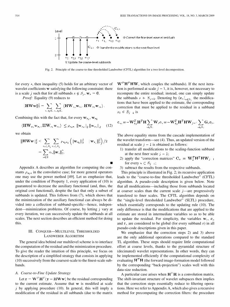
Fig. 2. Principle of the coarse-to-fine thresholded Landweber (CFTL) algorithm for a two-level decomposition.

for every , then inequality (5) holds for an arbitrary vector ofwavelet coefficients satisfying the following constraint: thereis a scale such that for all subbands , .

Proof: Equality (9) reduces to

Combining this with the fact that, for every ,

(12)

we obtain

Appendix A describes an algorithm for computing the con-stants in the convolutive case; for more general operatorsone may use the power method [49]. Let us emphasize that,under the condition of Property 1, every application of (10) isguaranteed to decrease the auxiliary functional (and, thus, theoriginal cost functional), despite the fact that only a subset ofsubbands is updated. This follows from (7), which shows thatthe minimization of the auxiliary functional can always be di-vided into a collection of subband-specific—hence, indepen-dent—minimization problems. Of course, by letting vary atevery iteration, we can successively update the subbands at allscales. The next section describes an efficient method for doingthis.

III. CONQUER—MULTILEVEL THRESHOLDED

LANDWEBER ALGORITHM

The general idea behind our multilevel scheme is to interlacethe computation of the residual and the minimization procedure.To give the reader the intuition of this principle, we focus onthe description of a simplified strategy that consists in applying(10) successively from the coarsest-scale to the finest-scale sub-bands.

A. Coarse-to-Fine Update Strategy

Let be the residual correspondingto the current estimate. Assume that is modified at scale

by applying procedure (10). In general, this will imply amodification of the residual in all subbands (due to the matrix

, which couples the subbands). If the next itera-tion is performed at scale , it is, however, not necessary torecompute the entire residual; instead, one can simply updatethe subbands . Denoting by the modifica-tions that have been applied to the estimate, the correspondingcorrection that must be applied to the residual in a subband

is

The above equality stems from the cascade implementation ofthe wavelet transform—see (4). Thus, an updated version of theresidual at scale is obtained as follows:

1) transfer all modifications to the scaling-function subbandat the next finer scale ;

2) apply the “correction matrices”for every ;

3) subtract the results from the respective subbands.This principle is illustrated in Fig. 2; its recursive application

leads to the “coarse-to-fine thresholded Landweber” (CFTL)algorithm. A pseudo-code description is given below. Notethat all modifications—including those from subbands locatedat coarser scales than the current scale —are progressivelytransfered to finer scales. The CFTL algorithm depends onthe “single-level thresholded Landweber” (SLTL) procedure,which essentially corresponds to the updating rule (10). Theonly difference is that the modifications that are applied to theestimate are stored in intermediate variables so as to be ableto update the residual. For simplicity, the variables ,and are considered to be global (for every subband ) in allpseudo-code descriptions given in this paper.

We emphasize that the correction steps 2) and 3) aboveare the only additional operations compared to the standardTL algorithm. These steps should require little computationaleffort at coarse levels, thanks to the pyramidal structure of(decimated) wavelet representations. In other words, they canbe implemented efficiently if the computational complexity ofevaluating (the forward image-formation model followedby the corresponding “back-projection”) scales well with thisdata-size reduction.

A particular case arises when is a convolution matrix.The shift-invariant structure of wavelet subspaces then impliesthat the correction steps essentially reduce to filtering opera-tions. Here we refer to Appendix A, which also gives a recursivemethod for precomputing the correction filters: the procedure


is akin to a wavelet decomposition of the convolution kernelcorresponding to and is easily implementable in the fre-quency domain (see also [50]). The correction steps can be im-plemented with a linear cost provided that we store the DFTsof the individual wavelet subbands; the actual wavelet coeffi-cients are only needed for the thresholding operations and canbe computed efficiently using the FFT algorithm. In terms ofcomputational work, one iteration of our algorithm is, there-fore, equivalent to two FFTs per subband, which amounts totwo FFTs at the signal level (level 0). The overall complexity ofa full coarse-to-fine run is, thus, on the same order as one runof the standard TL algorithm, which also requires two FFTs periteration in the convolutive case.

With a slight anticipation of the next subsection, we concludethis part by noting that multigrid methodologies sometimesadvocate the approximate resolution of coarse-level problems[15]. In the particular situations where the wavelet subbandsare weakly coupled by the image-formation operator, wehave indeed observed that the CFTL algorithm convergeseven if the correction steps are not applied; that is, if theresidual is only updated at the beginning of the iteration loop.This amounts to applying (8) using fairly optimistic boundconstants—without guarantee that the cost functional is mono-tonically decreased—and calls for further investigation. Thisapproach may turn out to be useful when dealing with compleximage-formation models that can not be evaluated easily atcoarse levels.

Algorithm 1

For every :•••

Algorithm 2 CFTL

• Initialization:— Choose some initial estimate— Compute its wavelet decomposition:

• Repeat times:— Compute the residual: for every ,

— Update the subbands from coarse to fine levels, i.e., for, :

• Update the subbands at the current level:• Transfer the modifications to the next finer level:

• If , correct the residual for the waveletsubbands at the next finer level:for every ,

— Set• Return

B. General Multilevel Scheme

With the previous algorithm in mind, one can conceive ofmore general multilevel strategies for updating the differentscales in a more flexible manner. In Appendix B, we provide apseudo-code description of a method that is strongly inspired bythe multigrid paradigm. However, there is one fundamental dif-ference: traditional multigrid schemes typically cycle throughnested subspaces corresponding to increasingly coarse dis-cretizations of the original inverse problem [51]. In the presentcontext, we successively update the wavelet subbands at everyscale; that is, we reinterpret the different scales of the wavelettransform as a multilevel representation of the inverse problem.The corresponding subspaces are not nested—they contain theoscillating components corresponding to the difference betweensuccessive coarse-level approximations. Incidentally, early at-tempts to apply the multigrid paradigm to image-restorationproblems remained relatively unsuccessful because they wereconcentrating on slowly oscillating components [52], [53].

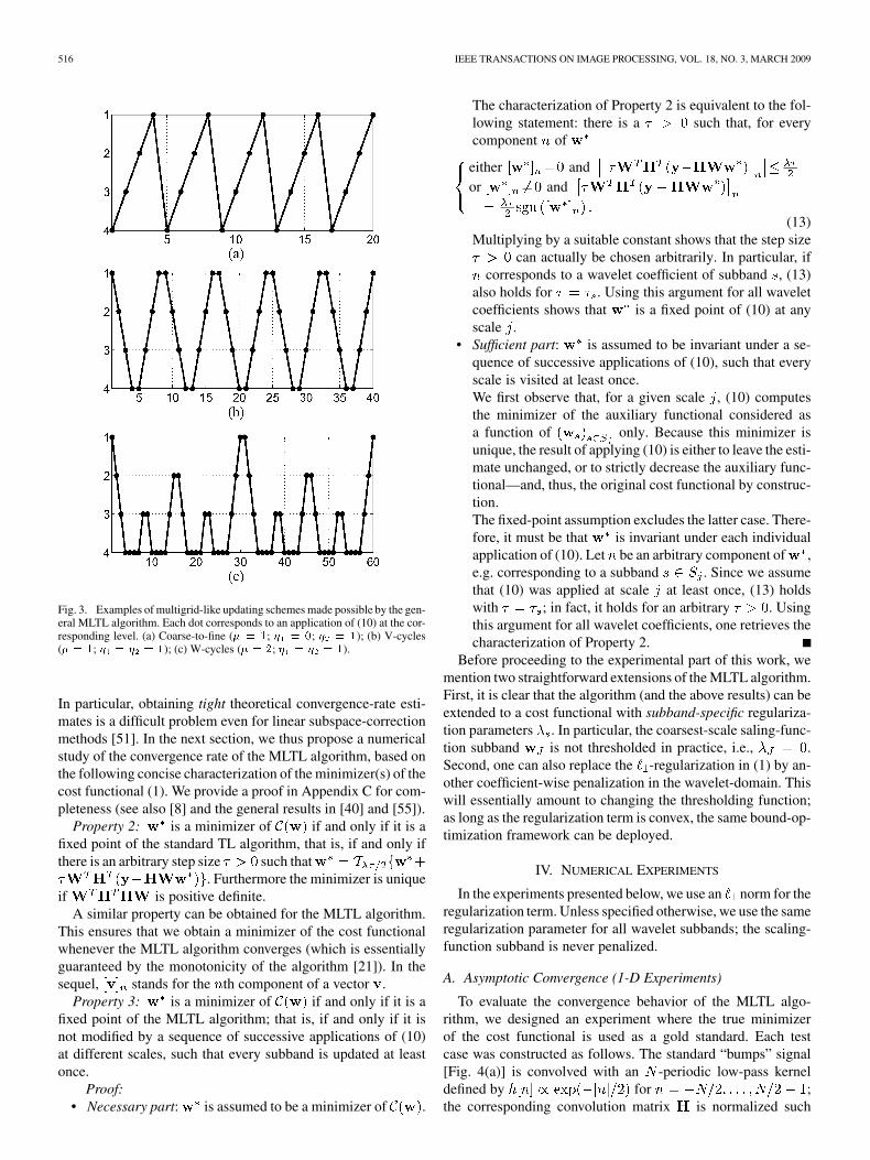
We have tried to specify the “multilevel thresholdedLandweber” (MLTL) algorithm in a modular way that isrelatively close to machine implementation. Its main buildingblock, UpdateLevel , depends on three parameters so asto be able to mimic typical multigrid schemes (see Fig. 3).The parameters are, thus, named , and , followingthe conventions of the multigrid literature [15], [54]. In theparticular case , and , one retrieves thecoarse-to-fine update described in the preceding subsection[Fig. 3(a)]. However, we should note that the MLTL algorithmis numerically (slightly) more stable, because the current esti-mate is explicitely reconstructed from its wavelet coefficientsat every iteration.

The different modules of Appendix B can be summarized asfollows.

• UpdateResidual : updates the residual for the subbandsat scale (if needed). Uses the correction principle of Fig.2 if the wavelet subbands have not been modified so far.Otherwise, the update is performed by temporarily movingup to the next finer scaling-function subband.

• UpdateLevel : recursive procedure which— updates the subbands at coarser scales by calling itself

times;— updates the subbands at scale by calling (the

number of updates before and after a recursive call arefixed by and , respectively).

Note that the procedure must compute the current residualfor the scaling-function subband at scale before callingitself. This is either done by applying the correction prin-ciple of Fig. 2 in the opposite direction (from the waveletsubbands to the scaling-function subband), or by going tothe next finer scale using UpdateResidual .

• MLTL: main routine that performs initialization tasksfollowed by several iterations of the update procedure.One may devise even more general—e.g. “full multigrid”[14]—schemes by adapting this routine.

C. Fixed-Point Property

A comprehensive study of the convergence properties of theMLTL algorithm is well beyond the scope of the present work.


Fig. 3. Examples of multigrid-like updating schemes made possible by the gen-eral MLTL algorithm. Each dot corresponds to an application of (10) at the cor-responding level. (a) Coarse-to-fine (� � �; � � �; � � �); (b) V-cycles(� � �; � � � � �); (c) W-cycles (� � �; � � � � �).

In particular, obtaining tight theoretical convergence-rate esti-mates is a difficult problem even for linear subspace-correctionmethods [51]. In the next section, we thus propose a numericalstudy of the convergence rate of the MLTL algorithm, based onthe following concise characterization of the minimizer(s) of thecost functional (1). We provide a proof in Appendix C for com-pleteness (see also [8] and the general results in [40] and [55]).

Property 2: is a minimizer of if and only if it is afixed point of the standard TL algorithm, that is, if and only ifthere is an arbitrary step size such that

. Furthermore the minimizer is uniqueif is positive definite.

A similar property can be obtained for the MLTL algorithm.This ensures that we obtain a minimizer of the cost functionalwhenever the MLTL algorithm converges (which is essentiallyguaranteed by the monotonicity of the algorithm [21]). In thesequel, stands for the th component of a vector .

Property 3: is a minimizer of if and only if it is afixed point of the MLTL algorithm; that is, if and only if it isnot modified by a sequence of successive applications of (10)at different scales, such that every subband is updated at leastonce.

Proof:• Necessary part: is assumed to be a minimizer of .

The characterization of Property 2 is equivalent to the fol-lowing statement: there is a such that, for everycomponent of

either andor and

(13)Multiplying by a suitable constant shows that the step size

can actually be chosen arbitrarily. In particular, ifcorresponds to a wavelet coefficient of subband , (13)

also holds for . Using this argument for all waveletcoefficients shows that is a fixed point of (10) at anyscale .

• Sufficient part: is assumed to be invariant under a se-quence of successive applications of (10), such that everyscale is visited at least once.We first observe that, for a given scale , (10) computesthe minimizer of the auxiliary functional considered asa function of only. Because this minimizer isunique, the result of applying (10) is either to leave the esti-mate unchanged, or to strictly decrease the auxiliary func-tional—and, thus, the original cost functional by construc-tion.The fixed-point assumption excludes the latter case. There-fore, it must be that is invariant under each individualapplication of (10). Let be an arbitrary component of ,e.g. corresponding to a subband . Since we assumethat (10) was applied at scale at least once, (13) holdswith ; in fact, it holds for an arbitrary . Usingthis argument for all wavelet coefficients, one retrieves thecharacterization of Property 2.

Before proceeding to the experimental part of this work, wemention two straightforward extensions of the MLTL algorithm.First, it is clear that the algorithm (and the above results) can beextended to a cost functional with subband-specific regulariza-tion parameters . In particular, the coarsest-scale saling-func-tion subband is not thresholded in practice, i.e., .Second, one can also replace the -regularization in (1) by an-other coefficient-wise penalization in the wavelet-domain. Thiswill essentially amount to changing the thresholding function;as long as the regularization term is convex, the same bound-op-timization framework can be deployed.

IV. NUMERICAL EXPERIMENTS

In the experiments presented below, we use an norm for theregularization term. Unless specified otherwise, we use the sameregularization parameter for all wavelet subbands; the scaling-function subband is never penalized.

A. Asymptotic Convergence (1-D Experiments)

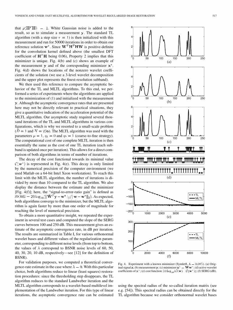
To evaluate the convergence behavior of the MLTL algo-rithm, we designed an experiment where the true minimizerof the cost functional is used as a gold standard. Each testcase was constructed as follows. The standard “bumps” signal[Fig. 4(a)] is convolved with an -periodic low-pass kerneldefined by for ;the corresponding convolution matrix is normalized such


that . White Gaussian noise is added to theresult, so as to simulate a measurement . The standard TLalgorithm (with a step size ) is then initialized with thismeasurement and run for 50000 iterations in order to obtain ourreference solution . Since is positive-definitefor the convolution kernel defined above (the smallest DFTcoefficient of being 0.06), Property 2 implies that thisminimizer is unique. Fig. 4(b) and (c) shows an example ofthe measurement and of the corresponding minimizer .Fig. 4(d) shows the locations of the nonzero wavelet coeffi-cients of the solution (we use a 3-level wavelet decompositionand the upper plot represents the finest-resolution subband).

We then used this reference to compare the asymptotic be-havior of the TL and MLTL algorithms. To this end, we per-formed a series of experiments where the algorithms are appliedto the minimization of (1) and initialized with the measurement

. Although the asymptotic convergence rates that are presentedhere may not be directly relevant to practical situations, theygive a quantitative indication of the acceleration potential of theMLTL algorithm. Our asymptotic study required several thou-sand iterations of the TL and MLTL algorithms in various con-figurations, which is why we resorted to a small-scale problem( and ). The MLTL algorithm was used with theparameters , and (coarse-to-fine strategy).The computational cost of one complete MLTL iteration is thenessentially the same as the cost of one TL iteration (each sub-band is updated once per iteration). This allows for a direct com-parison of both algorithms in terms of number of iterations.

The decay of the cost functional towards its minimal valueis represented in Fig. 4(e). This decay is only limited

by the numerical precision of the computer environment (weused Matlab on a 64-bit Intel Xeon workstation). To reach thislimit with the MLTL algorithm, the number of iterations is di-vided by more than 10 compared to the TL algorithm. We alsodisplay the distance between the estimate and the minimizer[Fig. 4(f)]; here, the “signal-to-error-ratio gain” is defined as

. As expected,both algorithms converge to the minimizer, but the MLTL algo-rithm is again faster by more than one order of magnitude forreaching the level of numerical precision.

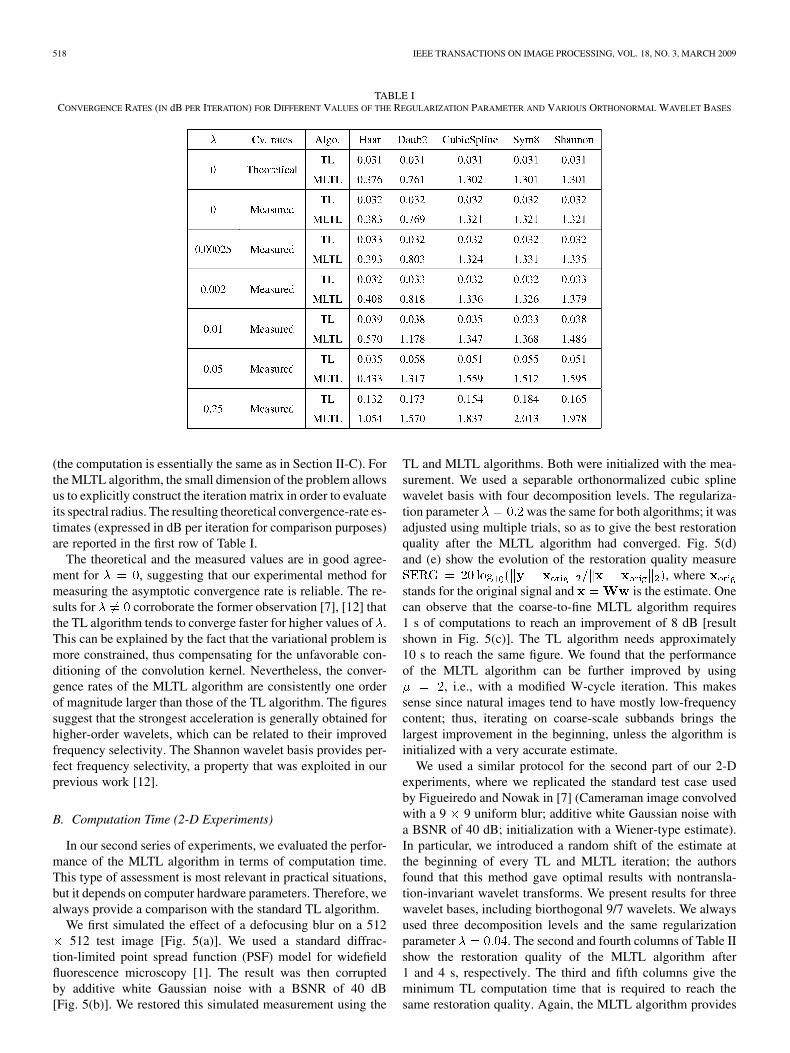
To obtain a more quantitative insight, we repeated the exper-iment in several test cases and computed the slope of the SERGcurves between 100 and 250 dB. This measurement gives an es-timate of the asymptotic convergence rate, in dB per iteration.The results are summarized in Table I, for various orthonormalwavelet bases and different values of the regularization param-eter, corresponding to different noise levels (from top to bottom,the values of correspond to BSNR noise levels of 60, 50,40, 30, 20, 10 dB, respectively—see [12] for the definition ofBSNR).

For validation purposes, we computed a theoretical conver-gence-rate estimate in the case where . With this particularchoice, both algorithms reduce to linear (least squares) restora-tion procedures: since the thresholding step disappears, the TLalgorithm reduces to the standard Landweber iteration and theMLTL algorithm corresponds to a wavelet-based multilevel im-plementation of the Landweber iteration. For this type of lineariterations, the asymptotic convergence rate can be estimated

Fig. 4. Experiment with a known minimizer (Symlet8, � � ��). (a) Orig-inal signal�; (b) measurement�; (c) minimizer� �� ; (d) active waveletcoefficients of � ; (e) cost function: �� ; (f) SERG (dB).

using the spectral radius of the so-called iteration matrix (seee.g. [54]). This spectral radius can be obtained directly for theTL algorithm because we consider orthonormal wavelet bases


TABLE ICONVERGENCE RATES (IN dB PER ITERATION) FOR DIFFERENT VALUES OF THE REGULARIZATION PARAMETER AND VARIOUS ORTHONORMAL WAVELET BASES

(the computation is essentially the same as in Section II-C). Forthe MLTL algorithm, the small dimension of the problem allowsus to explicitly construct the iteration matrix in order to evaluateits spectral radius. The resulting theoretical convergence-rate es-timates (expressed in dB per iteration for comparison purposes)are reported in the first row of Table I.

The theoretical and the measured values are in good agree-ment for , suggesting that our experimental method formeasuring the asymptotic convergence rate is reliable. The re-sults for corroborate the former observation [7], [12] thatthe TL algorithm tends to converge faster for higher values of .This can be explained by the fact that the variational problem ismore constrained, thus compensating for the unfavorable con-ditioning of the convolution kernel. Nevertheless, the conver-gence rates of the MLTL algorithm are consistently one orderof magnitude larger than those of the TL algorithm. The figuressuggest that the strongest acceleration is generally obtained forhigher-order wavelets, which can be related to their improvedfrequency selectivity. The Shannon wavelet basis provides per-fect frequency selectivity, a property that was exploited in ourprevious work [12].

B. Computation Time (2-D Experiments)

In our second series of experiments, we evaluated the perfor-mance of the MLTL algorithm in terms of computation time.This type of assessment is most relevant in practical situations,but it depends on computer hardware parameters. Therefore, wealways provide a comparison with the standard TL algorithm.

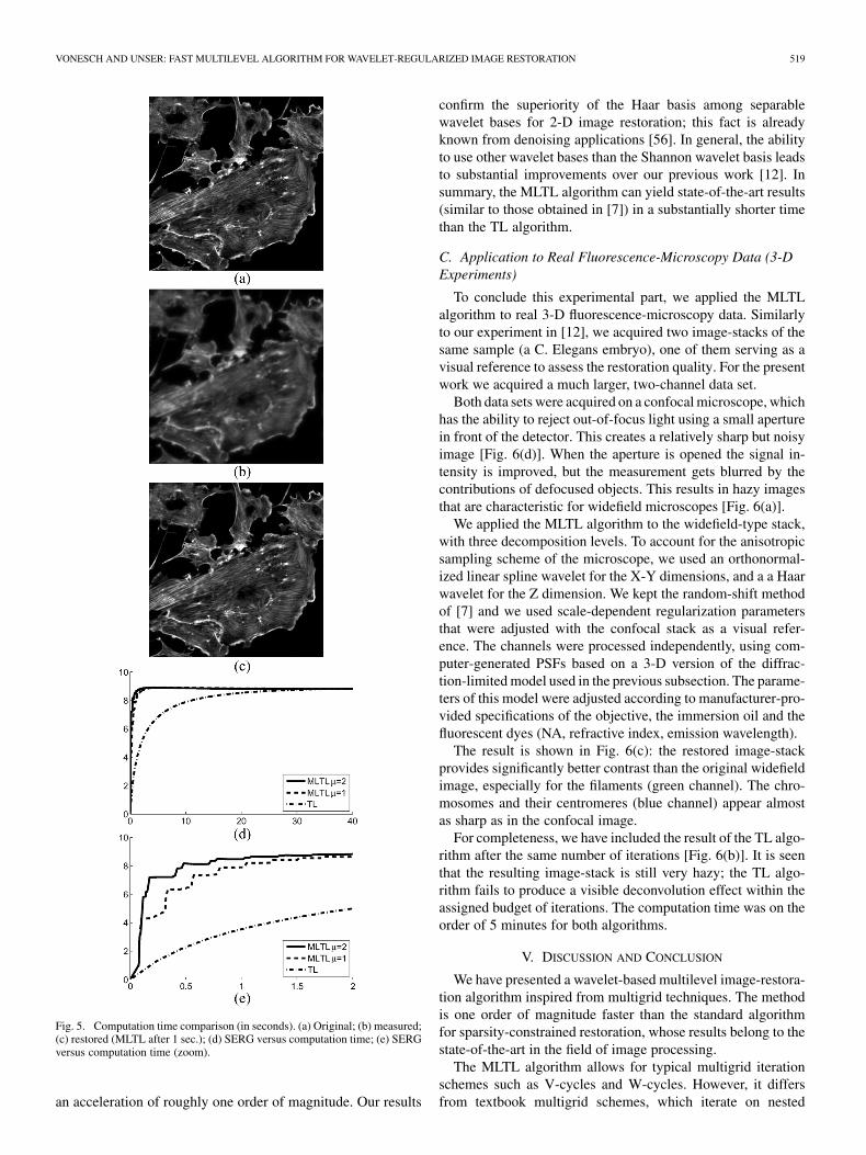
We first simulated the effect of a defocusing blur on a 512512 test image [Fig. 5(a)]. We used a standard diffrac-

tion-limited point spread function (PSF) model for widefieldfluorescence microscopy [1]. The result was then corruptedby additive white Gaussian noise with a BSNR of 40 dB[Fig. 5(b)]. We restored this simulated measurement using the

TL and MLTL algorithms. Both were initialized with the mea-surement. We used a separable orthonormalized cubic splinewavelet basis with four decomposition levels. The regulariza-tion parameter was the same for both algorithms; it wasadjusted using multiple trials, so as to give the best restorationquality after the MLTL algorithm had converged. Fig. 5(d)and (e) show the evolution of the restoration quality measure

, wherestands for the original signal and is the estimate. Onecan observe that the coarse-to-fine MLTL algorithm requires1 s of computations to reach an improvement of 8 dB [resultshown in Fig. 5(c)]. The TL algorithm needs approximately10 s to reach the same figure. We found that the performanceof the MLTL algorithm can be further improved by using

, i.e., with a modified W-cycle iteration. This makessense since natural images tend to have mostly low-frequencycontent; thus, iterating on coarse-scale subbands brings thelargest improvement in the beginning, unless the algorithm isinitialized with a very accurate estimate.

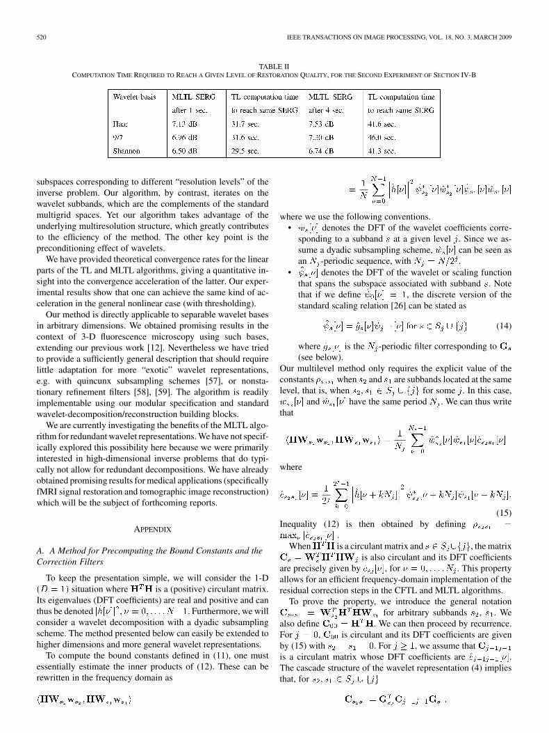
We used a similar protocol for the second part of our 2-Dexperiments, where we replicated the standard test case usedby Figueiredo and Nowak in [7] (Cameraman image convolvedwith a 9 9 uniform blur; additive white Gaussian noise witha BSNR of 40 dB; initialization with a Wiener-type estimate).In particular, we introduced a random shift of the estimate atthe beginning of every TL and MLTL iteration; the authorsfound that this method gave optimal results with nontransla-tion-invariant wavelet transforms. We present results for threewavelet bases, including biorthogonal 9/7 wavelets. We alwaysused three decomposition levels and the same regularizationparameter . The second and fourth columns of Table IIshow the restoration quality of the MLTL algorithm after1 and 4 s, respectively. The third and fifth columns give theminimum TL computation time that is required to reach thesame restoration quality. Again, the MLTL algorithm provides


Fig. 5. Computation time comparison (in seconds). (a) Original; (b) measured;(c) restored (MLTL after 1 sec.); (d) SERG versus computation time; (e) SERGversus computation time (zoom).

an acceleration of roughly one order of magnitude. Our results

confirm the superiority of the Haar basis among separablewavelet bases for 2-D image restoration; this fact is alreadyknown from denoising applications [56]. In general, the abilityto use other wavelet bases than the Shannon wavelet basis leadsto substantial improvements over our previous work [12]. Insummary, the MLTL algorithm can yield state-of-the-art results(similar to those obtained in [7]) in a substantially shorter timethan the TL algorithm.

C. Application to Real Fluorescence-Microscopy Data (3-DExperiments)

To conclude this experimental part, we applied the MLTLalgorithm to real 3-D fluorescence-microscopy data. Similarlyto our experiment in [12], we acquired two image-stacks of thesame sample (a C. Elegans embryo), one of them serving as avisual reference to assess the restoration quality. For the presentwork we acquired a much larger, two-channel data set.

Both data sets were acquired on a confocal microscope, whichhas the ability to reject out-of-focus light using a small aperturein front of the detector. This creates a relatively sharp but noisyimage [Fig. 6(d)]. When the aperture is opened the signal in-tensity is improved, but the measurement gets blurred by thecontributions of defocused objects. This results in hazy imagesthat are characteristic for widefield microscopes [Fig. 6(a)].

We applied the MLTL algorithm to the widefield-type stack,with three decomposition levels. To account for the anisotropicsampling scheme of the microscope, we used an orthonormal-ized linear spline wavelet for the X-Y dimensions, and a a Haarwavelet for the Z dimension. We kept the random-shift methodof [7] and we used scale-dependent regularization parametersthat were adjusted with the confocal stack as a visual refer-ence. The channels were processed independently, using com-puter-generated PSFs based on a 3-D version of the diffrac-tion-limited model used in the previous subsection. The parame-ters of this model were adjusted according to manufacturer-pro-vided specifications of the objective, the immersion oil and thefluorescent dyes (NA, refractive index, emission wavelength).

The result is shown in Fig. 6(c): the restored image-stackprovides significantly better contrast than the original widefieldimage, especially for the filaments (green channel). The chro-mosomes and their centromeres (blue channel) appear almostas sharp as in the confocal image.

For completeness, we have included the result of the TL algo-rithm after the same number of iterations [Fig. 6(b)]. It is seenthat the resulting image-stack is still very hazy; the TL algo-rithm fails to produce a visible deconvolution effect within theassigned budget of iterations. The computation time was on theorder of 5 minutes for both algorithms.

V. DISCUSSION AND CONCLUSION

We have presented a wavelet-based multilevel image-restora-tion algorithm inspired from multigrid techniques. The methodis one order of magnitude faster than the standard algorithmfor sparsity-constrained restoration, whose results belong to thestate-of-the-art in the field of image processing.

The MLTL algorithm allows for typical multigrid iterationschemes such as V-cycles and W-cycles. However, it differsfrom textbook multigrid schemes, which iterate on nested


TABLE IICOMPUTATION TIME REQUIRED TO REACH A GIVEN LEVEL OF RESTORATION QUALITY, FOR THE SECOND EXPERIMENT OF SECTION IV-B

subspaces corresponding to different “resolution levels” of theinverse problem. Our algorithm, by contrast, iterates on thewavelet subbands, which are the complements of the standardmultigrid spaces. Yet our algorithm takes advantage of theunderlying multiresolution structure, which greatly contributesto the efficiency of the method. The other key point is thepreconditioning effect of wavelets.

We have provided theoretical convergence rates for the linearparts of the TL and MLTL algorithms, giving a quantitative in-sight into the convergence acceleration of the latter. Our exper-imental results show that one can achieve the same kind of ac-celeration in the general nonlinear case (with thresholding).

Our method is directly applicable to separable wavelet basesin arbitrary dimensions. We obtained promising results in thecontext of 3-D fluorescence microscopy using such bases,extending our previous work [12]. Nevertheless we have triedto provide a sufficiently general description that should requirelittle adaptation for more “exotic” wavelet representations,e.g. with quincunx subsampling schemes [57], or nonsta-tionary refinement filters [58], [59]. The algorithm is readilyimplementable using our modular specification and standardwavelet-decomposition/reconstruction building blocks.

We are currently investigating the benefits of the MLTL algo-rithm for redundant wavelet representations. We have not specif-ically explored this possibility here because we were primarilyinterested in high-dimensional inverse problems that do typi-cally not allow for redundant decompositions. We have alreadyobtained promising results for medical applications (specificallyfMRI signal restoration and tomographic image reconstruction)which will be the subject of forthcoming reports.

APPENDIX

A. A Method for Precomputing the Bound Constants and theCorrection Filters

To keep the presentation simple, we will consider the 1-Dsituation where is a (positive) circulant matrix.

Its eigenvalues (DFT coefficients) are real and positive and canthus be denoted , . Furthermore, we willconsider a wavelet decomposition with a dyadic subsamplingscheme. The method presented below can easily be extended tohigher dimensions and more general wavelet representations.

To compute the bound constants defined in (11), one mustessentially estimate the inner products of (12). These can berewritten in the frequency domain as

where we use the following conventions.• denotes the DFT of the wavelet coefficients corre-

sponding to a subband at a given level . Since we as-sume a dyadic subsampling scheme, can be seen asan -periodic sequence, with .

• denotes the DFT of the wavelet or scaling functionthat spans the subspace associated with subband . Notethat if we define , the discrete version of thestandard scaling relation [26] can be stated as

(14)

where is the -periodic filter corresponding to(see below).

Our multilevel method only requires the explicit value of theconstants when and are subbands located at the samelevel, that is, when for some . In this case,

and have the same period . We can thus writethat

where

(15)Inequality (12) is then obtained by defining

.When is a circulant matrix and , the matrix

is also circulant and its DFT coefficientsare precisely given by , for . This propertyallows for an efficient frequency-domain implementation of theresidual correction steps in the CFTL and MLTL algorithms.

To prove the property, we introduce the general notationfor arbitrary subbands , . We

also define . We can then proceed by recurrence.For , is circulant and its DFT coefficients are givenby (15) with . For , we assume thatis a circulant matrix whose DFT coefficients are .The cascade structure of the wavelet representation (4) impliesthat, for


For a given subband , the algorithmic interpretation of is1) dyadic upsampling, followed by 2) filtering with . Itstranspose stands for 1) filtering with , followed by2) dyadic downsampling. Therefore, is also a circulantmatrix with DFT coefficients

(16)The equality stems from definition (15) for , and fromthe scaling relation (14); this completes the proof by recurrence.

Note that relation (16) provides a way to recursively computethe filters and the corresponding constants (with

).

B. Pseudo-Code Description of the General MLTL Algorithm

As in the previous subsection, we use the notation. The general MLTL algorithm uses both the

matrices and , for . It is useful to ob-serve that : in the convolutive case, this implies that

.

Algorithm 3 UpdateResidual

• If for some :—— For every , .

• Otherwise, if : for every , .

Algorithm 4 UpdateLevel

• Initialization:— For every , .— For every , .

• Repeat times:— Repeat times:

• UpdateResidual .• SLTL .

— If :• If for some :

• If , UpdateResidual .• Otherwise, .

• .• UpdateLevel .• .

— Repeat times:• UpdateResidual .• SLTL .

• .

Algorithm 5 MLTL

• Initialization:— Choose some initial estimate and set .

Fig. 6. Three-dimensional deconvolution results (maximum-intensity projec-tions of �� image stacks). (a) Original widefield stack (input data);(b) deconvolution result after 15 TL iterations; (c) deconvolution result after 15MLTL iterations; (d) confocal reference stack.

— Compute its wavelet decomposition (keeping thecoarse approximations):for , for every ,

.


• Repeat times:— .— UpdateLevel(1).

• Set and return .

C. Proof of Property 2

A short computation reveals that

(17)

where and are arbitrary vectors of wavelet coefficients.• Necessary part: we assume that for every

.— Suppose that for

some . Given a real and strictly positive constant , wedefine the vector by

ifotherwise.

In view of (17), can always be chosen such that, a contradiction. Therefore, it must be

that for every .— Choosing and inserting into

(17) gives the necessary condition

If it were true that, we could find a sufficiently small such

that this necessary condition is violated. Thus, it must bethat .Since for every , itfollows thatwhenever .

The combination of both results is equivalent to the fixed-point property.

• Sufficient part: is assumed to be a fixed point of the TLalgorithm.We use the same equivalence:— Since

whenever , we know thatand (17) reduces to

— Since for every , itfollows that

This also shows the unicity of the minimizer whenis positive definite.

REFERENCES

[1] C. Vonesch, F. Aguet, J.-L. Vonesch, and M. Unser, “The colored rev-olution of bioimaging,” IEEE Signal Process. Mag., vol. 23, no. 3, pp.20–31, May 2006.

[2] P. Sarder and A. Nehorai, “Deconvolution methods for 3-D fluores-cence microscopy images,” IEEE Signal Process. Mag., vol. 23, no. 3,pp. 32–45, May 2006.

[3] A. K. Louis, “Medical imaging: State of the art and future develop-ment,” Inv. Probl., vol. 8, no. 5, pp. 709–738, Oct. 1992.

[4] Handbook of Medical Imaging: Physics and Psychophysics, J. Beutel,H. L. Kundel, and R. L. Van Metter, Eds. Bellingham, WA: SPIE,Feb. 2000, vol. 1.

[5] R. Molina, J. Nunez, F. J. Cortijo, and J. Mateos, “Image restoration inastronomy: A Bayesian perspective,” IEEE Signal Process. Mag., vol.18, no. 2, pp. 11–29, Mar. 2001.

[6] J. L. Starck, E. Pantin, and F. Murtagh, “Deconvolution in astronomy:A review,” Pub. Astron. Soc. Pacific, vol. 114, no. 800, pp. 1051–1069,Oct. 2002.

[7] M. A. T. Figueiredoa and R. D. Nowak, “An EM algorithm for wavelet-based image restoration,” IEEE Trans. Image Process., vol. 12, no. 8,pp. 906–916, Aug. 2003.

[8] I. Daubechies, M. Defrise, and C. De Mol, “An iterative thresholdingalgorithm for linear inverse problems with a sparsity constraint,”Commun. Pure Appl. Math., vol. 57, no. 11, pp. 1413–1457, Aug.2004.

[9] J. Bect, L. Blanc-Féraud, G. Aubert, and A. Chambolle, “A � -unifiedvariational framework for image restoration,” in Proc. ECCV, 2004,vol. 3024, pp. 1–13, Part IV.

[10] I. Loris, G. Nolet, I. Daubechies, and F. A. Dahlen, “Tomographic in-version using � -regularization of wavelet coefficients,” Geophys. J.Int., vol. 170, no. 1, pp. 359–370, July 2007.

[11] J. M. Bioucas-Dias and M. A. T. Figueiredo, “A new TwIST: Two-step iterative shrinkage/thresholding algorithms for image restoration,”IEEE Trans. Image Process., vol. 16, no. 12, pp. 2992–3004, Dec. 2007.

[12] C. Vonesch and M. Unser, “A fast thresholded Landweber algorithmfor wavelet-regularized multidimensional deconvolution,” IEEE Trans.Image Process., vol. 17, no. 4, pp. 539–549, Apr. 2008.

[13] S. Mallat, “A theory for multiresolution signal decomposition: Thewavelet representation,” IEEE Trans. Pattern Anal. Mach. Intell., vol.11, no. 7, pp. 674–693, Jul. 1989.

[14] W. Hackbusch, Multi-Grid Methods and Applications. Berlin, Ger-many: Springer-Verlag, 1985, vol. 4, Springer Ser. Comput. Math.

[15] W. L. Briggs, V. E. Henson, and S. F. McCormick, A Multigrid Tuto-rial, 2nd ed. Philadelphia, PA: SIAM, 2000.

[16] W. M. Lawton, “Multiresolution properties of the wavelet Galerkin op-erator,” J. Math. Phys., vol. 32, no. 6, pp. 1440–1443, June 1991.

[17] Z. Cai and W. E, “Hierarchical method for elliptic problems usingwavelet,” Commun. Appl. Numer. Meth., vol. 8, no. 11, pp. 819–825,Nov. 1992.

[18] W. Dahmen and A. Kunoth, “Multilevel preconditioning,” Numer.Math., vol. 63, no. 1, pp. 315–344, Dec. 1992.

[19] W. L. Briggs and V. E. Henson, “Wavelets and multigrid,” SIAM J. Sci.Comput., vol. 14, no. 2, pp. 506–510, Mar. 1993.

[20] G. Wang, J. Zhang, and G.-W. Pan, “Solution of inverse problems inimage processing by wavelet expansion,” IEEE Trans. Image Process.,vol. 4, no. 5, pp. 579–593, May 1995.

[21] K. Lange, D. R. Hunter, and I. Yang, “Optimization transfer using sur-rogate objective functions,” J. Comput. Graph. Statist., vol. 9, no. 1,pp. 1–20, Mar. 2000.

[22] D. R. Hunter and K. Lange, “A tutorial on MM algorithms,” Amer.Statist., vol. 58, no. 1, pp. 30–37, Feb. 2004.

[23] M. W. Jacobson and J. A. Fessler, “An expanded theoretical treatmentof iteration-dependent majorize-minimize algorithms,” IEEE Trans.Image Process., vol. 16, no. 10, pp. 2411–2422, Oct. 2007.

[24] J. A. Fessler and A. O. Hero, “Space-alternating generalized expecta-tion-maximization algorithm,” IEEE Trans. Signal Process., vol. 42,no. 10, pp. 2664–2677, Oct. 1994.

[25] S. Oh, A. B. Milstein, C. A. Bouman, and K. J. Webb, “A general frame-work for nonlinear multigrid inversion,” IEEE Trans. Image Process.,vol. 14, no. 1, pp. 125–140, Jan. 2005.

[26] S. Mallat, A Wavelet Tour of Signal Processing. New York: Aca-demic, 1998.

[27] H. Yserentant, “On the multi-level splitting of finite element spaces,”Numer. Math., vol. 49, pp. 379–412, 1986.


[28] R. E. Bank, T. F. Dupont, and H. Yserentant, “The hierarchical basismultigrid method,” Numer. Math., vol. 52, no. 4, pp. 427–458, Jul.1988.

[29] P. S. Vassilevski and J. Wang, “Stabilizing the hierarchical basis byapproximate wavelets I: Theory,” Numer. Lin. Algebra Appl., vol. 4,no. 2, pp. 103–126, Mar./Apr. 1998.

[30] M. Bertero and P. Boccacci, Introduction to Inverse Problems inImaging. Bristol, U.K.: IOP, 1998.

[31] C. Christopoulos, A. Skodras, and T. Ebrahimi, “The JPEG2000 stillimage coding system: An overview,” IEEE Trans. Consum. Electron.,vol. 46, no. 4, pp. 1103–1127, Nov. 2000.

[32] C. De Mol and M. Defrise, “A note on wavelet-based inversion algo-rithms,” in Inverse Problems, Image Analysis and Medical Imaging, M.Z. Nashed and O. Scherzer, Eds. Providence, RI: American Mathe-matical Society, Nov. 2002, vol. 313, Contemporary Mathematics, pp.85–96, (Special Session on Interaction of Inverse Problems and ImageAnalysis. AMS Joint Mathematics Meetings, New Orleans, LA, Jan.10–13, 2001).

[33] R. D. Nowak and M. A. T. Figueiredo, “Fast wavelet-based image de-convolution using the EM algorithm,” presented at the 35th AsilomarConf. Signals, Systems and Computers, Pacific Grove, CA, Nov. 2001.

[34] J. L. Starck, D. L. Donoho, and E. J. Candès, “Astronomical imagerepresentation by the curvelet transform,” Astron. Astrophys., vol. 398,no. 2, pp. 785–800, February 2003.

[35] J.-L. Starck, M. K. Nguyen, and F. Murtagh, “Wavelets and curveletsfor image deconvolution: A combined approach,” Signal Process., vol.83, no. 10, pp. 2279–2283, October 2003.

[36] L. Landweber, “An iterative formula for Fredholm integral equationsof the first kind,” Amer. J. Math., vol. 73, no. 3, pp. 615–624, Jul. 1951.

[37] J. B. Weaver, Y. S. Xu, D. M. Healy, and L. D. Cromwell, “Filteringnoise from images with wavelet transforms,” Magn. Res. Med., vol. 21,no. 2, pp. 288–295, Oct. 1991.

[38] D. L. Donoho, “De-noising by soft-thresholding,” IEEE Trans. Inf.Theory, vol. 41, no. 3, pp. 613–627, May 1995.

[39] M. Liebling and M. Unser, “Autofocus for digital fresnel holograms byuse of a fresnelet-sparsity criterion,” J. Opt. Soc. Amer. A, vol. 21, no.12, pp. 2424–2430, Dec. 2004.

[40] C. Chaux, P. L. Combettes, J.-C. Pesquet, and V. R. Wajs, “A varia-tional formulation for frame-based inverse problems,” Inv. Probl., vol.23, no. 4, pp. 1495–1518, Aug. 2007.

[41] J. M. Bioucas-Dias, “Bayesian wavelet-based image deconvolution: AGEM algorithm exploiting a class of heavy-tailed priors,” IEEE Trans.Image Process., vol. 15, no. 4, pp. 937–951, Apr. 2006.

[42] M. A. T. Figueiredo, J. M. Bioucas-Dias, and R. D. Nowak, “Ma-jorization-minimization algorithms for wavelet-based image restora-tion,” IEEE Trans. Image Process., vol. 16, no. 12, pp. 2980–2991, Dec.2007.

[43] M. Elad, “Why simple shrinkage is still relevant for redundant repre-sentations?,” IEEE Trans. Inf. Theory, vol. 52, no. 12, pp. 5559–5569,Dec. 2006.

[44] M. Elad, B. Matalon, and M. Zibulevsky, “Coordinate and subspaceoptimization methods for linear least squares with non-quadratic regu-larization,” Appl. Comput. Harmon. Anal., vol. 23, no. 3, pp. 346–367,Nov. 2007.

[45] M. A. T. Figueiredo, R. D. Nowak, and S. J. Wright, “Gradient projec-tion for sparse reconstruction: Application to compressed sensing andother inverse problems,” IEEE J. Sel. Topics Signal Process., vol. 2007,no. 4, pp. 586–597, Dec. 2007.

[46] J. Friedman, T. Hastie, H. Höfling, and R. Tibshirani, “Pathwise co-ordinate optimization,” Ann. Appl. Statist., vol. 1, no. 2, pp. 302–332,Dec. 2007.

[47] M. Fornasier, “Domain decomposition methods for linear inverseproblems with sparsity constraints,” Inv. Probl., vol. 23, no. 6, pp.2505–2526, Dec. 2007.

[48] A. Chambolle, R. A. DeVore, N.-Y. Lee, and B. J. Lucier, “Non-linear wavelet image processing: Variational problems, compression,and noise removal through wavelet shrinkage,” IEEE Trans. ImageProcess., vol. 7, no. 3, pp. 319–335, Mar. 1998.

[49] G. H. Golub and C. F. van Loan, Matrix Computations. Baltimore,MD: Johns Hopkins Univ. Press, 1996.

[50] T. Blu and M. Unser, “The fractional spline wavelet transform: Def-inition and implementation,” in Proc. 25th IEEE Int. Conf. Acoust.,Speech, Signal Process., Jun. 2000, vol. I, pp. 512–515.

[51] J. Xu, “The method of subspace corrections,” J. Comput. Appl. Math.,vol. 128, no. 1–2, pp. 335–362, Mar. 2001.

[52] K. Zhou and C. K. Rushforth, “Image restoration using multigridmethods,” Appl. Opt., vol. 30, no. 20, pp. 2906–2912, Jul. 1991.

[53] T.-S. Pan and A. E. Yagle, “Numerical study of multigrid implementa-tions of some iterative image reconstruction algorithms,” IEEE Trans.Med. Imag., vol. 10, no. 4, pp. 572–288, Dec. 1991.

[54] W. Hackbusch, Iterative Solution of Large Sparse Systems of Equa-tions. New York: Springer-Verlag, 1994, vol. 95, Appl. Math. Sci.

[55] P. L. Combettes and V. R. Wajs, “Signal recovery by proximal for-ward-backward splitting,” Multiscale Model. Simul., vol. 4, no. 4, pp.1168–1200, 2005.

[56] T. Blu and F. Luisier, “The SURE-LET approach to image denoising,”IEEE Trans. Image Process., vol. 16, no. 11, pp. 2778–2786, Nov.2007.

[57] D. van de Ville, T. Blu, and M. Unser, “Isotropic polyharmonicB-splines: Scaling functions and wavelets,” IEEE Trans. ImageProcess., vol. 14, no. 11, pp. 1798–1813, Nov. 2005.

[58] I. Khalidov and M. Unser, “From differential equations to the construc-tion of new wavelet-like bases,” IEEE Trans. Signal Process., vol. 54,no. 4, pp. 1256–1267, Apr. 2006.

[59] C. Vonesch, T. Blu, and M. Unser, “Generalized Daubechies waveletfamilies,” IEEE Trans. Signal Process., vol. 55, no. 9, pp. 4415–4429,Sep. 2007.

Cédric Vonesch was born on April 14, 1981, inObernai, France. He spent one year studying at theEcole Nationale Supérieure des Télécommunica-tions, Paris, France, and graduated from the SwissInstitute of Technology, Lausanne (EPFL), in 2004,where he is currently pursuing the Ph.D. degree.

He is currently with the Biomedical ImagingGroup, EPFL. His research interests include mul-tiresolution and wavelet analysis, inverse problems,and applications to bioimaging.

Michael Unser (M’89–M’94–F’99) received theM.S. (summa cum laude) and Ph.D. degrees in elec-trical engineering in 1981 and 1984, respectively,from the Ecole Polytechnique Fédérale de Lausanne(EPFL), Switzerland.

From 1985 to 1997, he was a Scientist with theNational Institutes of Health, Bethesda, MD. He isnow a Full Professor and Director of the Biomed-ical Imaging Group at the EPFL. His main researcharea is biomedical image processing. He has a stronginterest in sampling theories, multiresolution algo-

rithms, wavelets, and the use of splines for image processing. He has publishedover 150 journal papers on those topics, and is one of ISIs Highly Cited authorsin Engineering (http://isihighlycited.com).

Dr. Unser has held the position of associate Editor-in-Chief (2003–2005) ofthe IEEE TRANSACTIONS ON MEDICAL IMAGING, for which he also served asan Associate Editor (1999–2002, 2006–2007). He has also served as an Asso-ciate Editor for the IEEE TRANSACTIONS ON IMAGE PROCESSING (1992–1995)and the IEEE SIGNAL PROCESSING LETTERS (1994–1998). He is currently amember of the editorial boards of Foundations and Trends in Signal Processing,the SIAM Journal of Imaging Sciences, and Sampling Theory in Signal andImage Processing. He co-organized the first IEEE International Symposiumon Biomedical Imaging (ISBI 2002). He was the founding chair of the tech-nical committee of the IEEE-SP Society on Bio Imaging and Signal Processing(BISP). He received the 1995 and 2003 Best Paper Awards and the 2000 Mag-azine Award from the IEEE Signal Processing Society.

a fast multilevel algorithm for wavelet-regularized image restoration

Documents