A Distributional Analysis of a Carbon Tax and Dividend in the United States

April 2017

Anders Fremstad1 and Mark Paul2

Abstract Although the vast majority of economists view a carbon tax as an efficient mechanism to reduce greenhouse gas emissions, the policy does not enjoy widespread public support. One reason for this is that economists have failed to adequately address the policy’s effect on household budgets. This paper models the distributional impacts of placing a $49 tax per ton on carbon in the United States. We combine carbon emissions data from the Energy Information Agency with the Input-Output tables from the Bureau of Economic Analysis to calculate the carbon intensity of each industry and commodity. We then analyze data from the Consumer Expenditure Survey to estimate how households would be affected by placing a price on carbon. A carbon tax would disproportionately burden low-income households, and using the carbon tax revenue to reduce taxes on labor leaves 59 percent of people worse off, including 75 percent of those in the bottom half of the income distribution. On the other hand, equal per capita dividends protect the purchasing power of 61 percent of all individuals, including 89 percent of those in the bottom half of the distribution. Many economists have dismissed a tax-and-dividend scheme on efficiency grounds, but we show that potential macroeconomic effects of tax cuts do little to protect the purchasing power of the poor. In an age of increasing inequality, we argue that providing all Americans with equal rebates is the most fair and politically-feasible policy. JEL Numbers: H22, H23, Q48, Q52, Q54, Q58 Keywords: Carbon Tax; Distribution; Tax; Environment; Climate Change; Global Warming; Fossil Fuels; Tax-and-Dividend We would like to thank James Boyce, Michael Ash, and participants at the 2016 EEA session on Carbon Pricing. We especially thank Arparna Mathur and Adele Morris for graciously sharing their methods with us.

1 Anders Fremstad, Department of Economics, Colorado State University, C306 Clark Building, Fort Collins, CO. (413) 820-8281 anders.fremstad@coloradostate.edu 2 Mark Paul, Samuel DuBois Cook Center for Social Equity, Duke University, Campus Box 104407, Erwin Mill Building, Durham, NC. (413) 230-9175 mark.paul@duke.edu

1 Introduction This paper examines the distributional impacts at the household level of placing an economy-wide

tax on carbon dioxide (CO2).3 Although the vast majority of economists support a carbon tax as an

efficient mechanism for reducing greenhouse gas emissions (IGM 2012), the policy has not been

implemented at the national level. Placing a tax on carbon would represent a substantial

reorganization of property rights, so how those rights are allocated is of great importance. We

estimate that a modest $49 tax per ton of CO2 would redistribute $144 billion in revenue per year,

while a robust $200 per ton tax could redistribute $588 billion per year. The paper assesses the

distributional implications of a carbon tax and various revenue-neutral recycling policies, including a

proportional labor tax cut, an Old-Age, Survivor, and Disability Insurance (OASDI) payroll tax cut,

and an equal per capita carbon dividend. We argue that a tax-and-dividend policy is the most

equitable option. It may also be politically feasible. While the GOP has opposed legislation to put a

price on carbon for nearly a decade, a recent report from the Climate Leadership Council,

coauthored by prominent Republicans and conservative economists, calls for a carbon tax in which

the revenues are rebated in equal lump-sum dividends (Baker et al. 2017).

Our analysis uses Input-Output tables to estimate the carbon intensity of 64 industries and

33 expenditure categories in the U.S. We assume the entire burden of the carbon tax is passed on to

consumers in the form of higher prices. Using the Consumer Expenditure Survey (CEX), we

calculate the carbon footprints of a representative sample of U.S. households, which allows us to

analyze the carbon tax burden across the income distribution. Similar to other researchers, we find

that placing a tax on carbon is regressive and taxes poor households at a higher rate than rich

households. However, we also find that 61 percent of people receive more money back than they

pay under a tax-and-dividend scheme (Boyce and Riddle 2007; Boyce and Riddle 2010; Williams et

al. 2014; Horowitz et al. 2017).

Although both academic research and the popular media have addressed the incidence of a

carbon tax, the core distributional findings across potential revenue recycling schemes remain

contested. Results have traditionally focused on the net cost of a policy for the “mean” household in

each income decile (Boyce and Riddle 2007; Boyce and Riddle 2011; Mathur and Morris 2014;

Williams 2014). However, this approach can be misleading. For example, we find that the mean

household in the bottom seven deciles is better off under a tax-and-dividend scheme; however, only 3 Our central analysis can also be interpreted as the distributional consequences of increasing the price of carbon through a cap-and-trade scheme in which permits sell for $49/tCO2.

54 percent of households in the seventh decile actually benefit from the policy. Our case for a tax-

and-dividend policy stresses that it maintains the purchasing power of most Americans in the

bottom half of the income distribution. Protecting the income of the lower class is vital given the

failure of economic policy to increase their incomes since 1980 (Piketty 2014).

Carbon dioxide is emitted primarily by burning fossil fuels. In 2014 major fossil fuels

accounted for 5,406 metric tons of carbon dioxide emissions in the U.S., with 41 percent of

emissions from burning petroleum products, 32 percent from burning coal, and 27 percent from

burning natural gas (EIA 2015). The release of CO2 into the atmosphere as a result of burning fossil

fuels for energy accounts for approximately 76 percent of U.S. greenhouse gas (GHG) emissions

(Horowitz et al. 2017), with the remainder of GHG emissions coming from sources such as

agriculture and livestock, cement production, fertilizer, and biomass burning (Pachauri et al. 2015).

While CO2 emissions have decreased 12 percent from their peak in the United States in 2007 (EIA

2015) they must be rapidly reduced to zero by 2100 to avoid extreme temperature change (Fawcett

et al. 2015).

Putting a tax on CO2 emissions via a carbon tax reduces demand for carbon intensive goods

and services, and it provides incentives for individuals and firms to make investments in renewable

energy and energy efficiency (EIA 2013). While the U.S. does not currently have a federal carbon

pricing scheme, several states have priced carbon using a carbon tax or a carbon cap.4 As of 2016

over 40 national jurisdictions, as well as over 20 cities, states, and regions,5 have a carbon pricing

mechanism in place, and China is currently piloting what will soon be the world’s largest cap-and-

permit system (World Bank 2016). Relative to other high productivity economies, the U.S. is

markedly behind in enacting environmental legislation that would correct this major pollution

externality (Williams 2016). While a carbon tax is but one policy option to reduce emissions, studies

have found that placing a price on emissions would be more cost-effective than other policy

options, such as increasing emissions standards, subsidizing renewable energy, or investing in

research and development (Fisher and Newell 2008; Williams 2016).

Under a carbon tax, households ultimately pay a tax for each ton of CO2 they directly or

4 These include California and the nine states involved in the Regional Greenhouse Gas Initiative (RGGI): Connecticut, Delaware, Maine, Maryland, Massachusetts, New Hampshire, New York, Rhode Island, and Vermont. Other states, including Oregon, Washington, and New York are considering initiatives that would place a tax on carbon. 5 For example, the Regional Greenhouse Gas Initiative (RGGI) is a multi-state effort to collectively cap carbon emissions from power plants, covering seven states in the Northeast. This paper focuses on an economy wide tax on carbon. Previous work by Grainger and Kolstad (2009) has shown that a carbon tax that only applies to energy, such as RGGI, is more regressive than an economy wide carbon tax.

indirectly generate. A carbon tax that is equal to the marginal social damage from the pollution can

improve social welfare.6 The United States Environmental Protection Agency (E.P.A.) and other

federal agencies use the social cost of carbon to estimate the climate benefits of rulemaking. If the

tax rate is set equal to marginal external damage, it ensures that the price of goods reflects their full

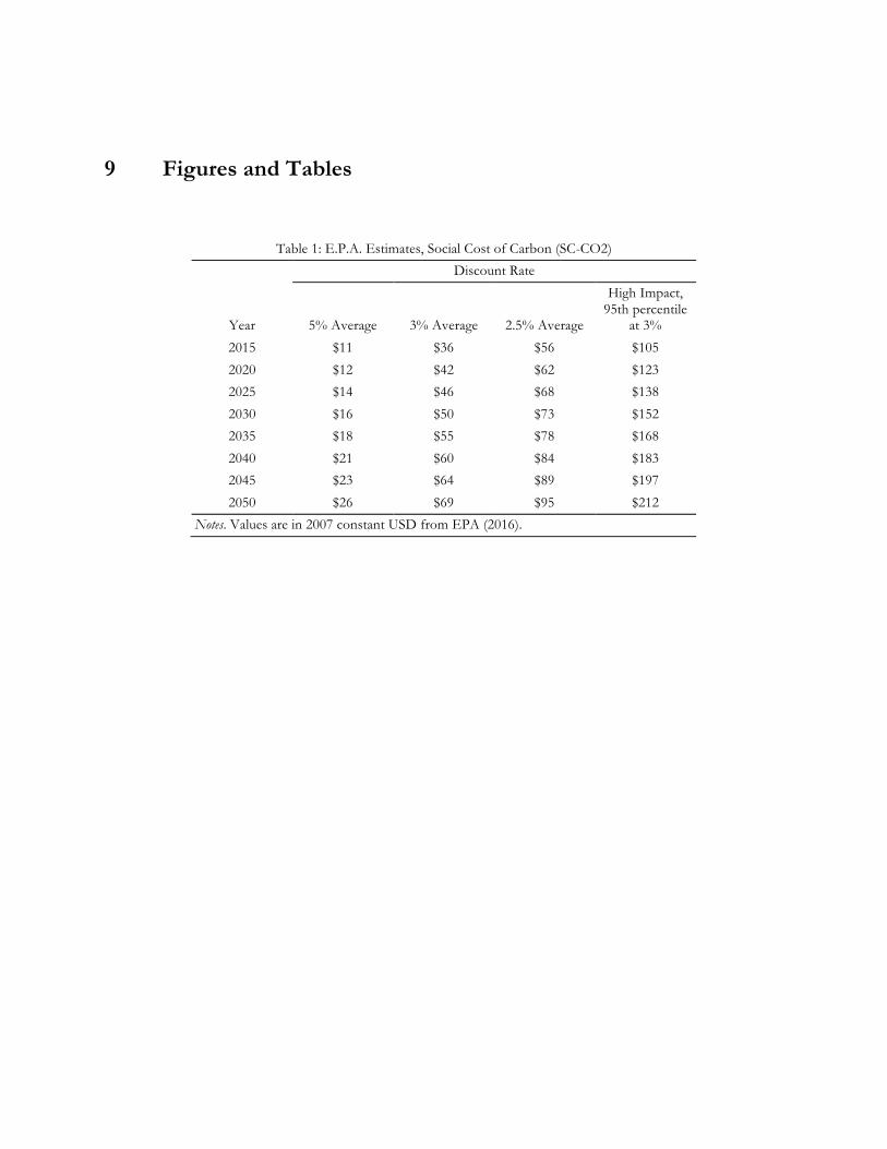
marginal social cost and internalizes the externality. The E.P.A.’s estimates for the social cost of

carbon are presented in Table 1 below. In this paper, we model a $49 carbon tax, which is equal to

the E.P.A.’s estimate of the social cost of carbon for 2020 using a 3 percent average discount rate,

and converted to 2016 dollars.7 This is equivalent to about a $0.49 tax per gallon of gasoline.8

[Insert Table 1 about here SCC]

This study presents new evidence on the distributional effects of a carbon tax when the

revenues are devoted to either a proportional decrease in labor tax rates, a OASDI payroll tax cut, or

equal per capita carbon dividends. Additionally, the paper attempts to clarify differences across

studies addressing the distributional implications of a carbon tax. While there is still no agreed-upon

method for analyzing the distribution of the tax burden, we work to build consensus by providing a

detailed description of our methods, publishing intermediate tables, and testing the robustness of

our conclusions. The following section reviews existing literature on the distributional impacts of

carbon taxes. Section 3 describes the data and methods utilized in this paper and presents carbon

intensities (in kgCO2/$) for 64 industries and 33 categories of consumer goods. Section 4 presents

the key distributional impact of competing carbon tax policies. Section 5 demonstrates that our core

results are similar when we analyze different years, rely on an alternative method to calculate carbon

intensities, and use income rather than consumption to sort households. Section 6 discusses our

results in the context of the equity-efficiency tradeoff and in terms of vertical and horizontal equity.

Section 7 concludes. 6 The case for carbon taxes are frequently made on the grounds of inter-generational equity. Rezai, Foley, and Taylor (2012) show that diverting investments to climate change mitigation can generate a Pareto improvement. Even if there is a tradeoff between the environmental interests current and future generations, there are immediate benefits to abatement. Boyce (2016) explores air quality co-benefits from placing a tax on carbon, and finds that substantial gains for present generations can be achieved through improvements in air quality. 7 The choice of a discount rate is crucial to determining the social cost of carbon, yet there is a lack of consensus on the appropriate discount rate used in climate economics. The lower the discount rate, the more important the outcomes in later years are - thus a discount rate of 3 percent as opposed to 5 percent (the two put forth by the E.P.A.) estimates a higher social cost of carbon. The EPA uses a 3 percent as the benchmark for policy. 8 A rule of thumb is that $1 per ton of CO2 is equivalent to roughly $0.01 per gallon of gasoline. This paper’s central CO2 intensity estimates suggest that a tax of $49/tCO2 would have raised gas prices by $0.56 per gallon of gasoline in 2013.

2 Background

The vast majority of studies find that the incidence of a carbon tax is regressive (Boyce and Riddle

2007; Hassett, Mathur, and Metcalf 2009; Dinan 2012; Mathur, Morris 2014; Williams et al. 2014;

Jorgenson et al. 2015), although two recent studies find that the burden of a carbon tax is fairly

constant across the income distribution (Cronin et al. 2017; Horowitz et al. 2017).9 Although most

studies agree that a carbon tax is a regressive tax, it is unclear how regressive the tax is. There is large

variation in the assumptions built into the various models to assess the incidence of such a tax, and

differences in assumptions explain the conflicting results.

Studies agree that the full distributional impact of a carbon tax depends crucially on what

policymakers do with the carbon tax revenue. Researchers have provided a range of

recommendations on how to best use the revenue. A review of the literature reveals a convergence

toward devoting carbon tax revenue to three schemes: cutting taxes on capital income, cutting taxes

on labor income, and rebating revenues in equal per-capita carbon dividends. Although most studies

find that paying everyone an equal per capita dividend is the most equitable option, many studies

argue for devoting revenue to reducing distortionary taxes on efficiency grounds (Dinan 2000;

Mathur and Morris 2014; Jorgenson 2015). The exact arguments depend largely on the models

employed in the analyses. While a range of models have been employed across the literature, the two

most common are computable general equilibrium (CGE) models and Input-Output models, such

as the one presented in this paper.

There are two main reasons that studies using CGE models tend to support devoting carbon

tax revenues to reducing taxes on capital or labor. First, these studies analyze the distributional

impact of a carbon tax over the very long run. Part of the reason for this is that CGE models allow

for firms and households to change their behavior over time in response to a carbon tax. Moreover,

researchers using CGE models tend to examine the impact of policies on lifetime earnings instead of

analyzing the immediate impact on household budgets (Jorgenson et al. 2015; Williams et al. 2014).

These overlapping generations models assume away a key component of intergenerational equity.

While a carbon tax will increase prices for everyone, Americans who are in or near retirement would

receive little benefit from cuts in labor or capital taxes. Overlapping generation models also provide

little practical guidance to voters, who are less concerned with how a carbon tax scheme may affect

their lifetime earnings, which are clouded by uncertainty, and more interested in how such a policy

9 See table 5 column 6 in Cronin et al. (2017) and Horowitz et al. (2017) table 6.

will affects their purchasing power across the next few years.

The second reason that CGE models tend to support devoting carbon tax revenues to tax

cuts is that they focus on the macroeconomic effects rather than the distributional impacts of tax

changes. CGE models suggest that there is a macroeconomic cost to devoting carbon tax revenues

to a carbon dividend instead of reducing taxes on capital. Jorgenson et al. (2015) estimate that

funding a carbon dividend reduces full consumption by about 0.3 percent, Goulder and Hafstead

(2013) find that it reduces GDP by 0.3 percent, and Williams et. al (2014) find that it reduces mean

welfare by 0.45 percent. As a result, the CGE models always find that the mean household is better

off in the long run when carbon tax revenues are devoted to cutting distortionary taxes instead of

paying for a carbon dividend (Jorgenson et al. 2015; Williams et al. 2014).

However, recent research challenges many of the assumptions underlying CGE models and

calls into question the plausibility of these macroeconomic effects. The argument for cutting

distortionary taxes is that it will increase economic activity, but work by Steinbaum and Bernstein

(2017) dispute this. Lower taxes on capital are supposed to spur economic growth through increased

investment, but Gutierrez and Philippon (2016) find that financial constraints are not the major

obstacle to greater investment. New empirical evidence also suggests that lowering the corporate tax

rate or raising access to cash for firms would likely result in larger payouts to shareholders rather

than increased investment by firms (Mason 2015).

Even if cuts to distortionary taxes would increase economic growth, it is not clear that those

gains would be equally distributed. The optimal tax rate literature argues that the burden of the

corporate income tax is shared between labor and capital (Piketty and Saez 2012), but recent

empirical work suggests the tax falls mostly on capital. For example, the U.S. Treasury Department

assigns 82 percent of the burden to capital income, while the Tax Policy Center assigns 80 percent to

capital. Others, such as the Joint Committee on Taxation, assign the entire burden of the tax to

capital in the short run, though the burden is shared between capital and labor in the long run.

Recent research by Clausing (2012, 2013) finds that the corporate tax is borne by the top of the

income and wealth distribution, observing “no robust link between corporate taxation and wages.”

The carbon tax literature is beginning to consider this new evidence. Horowitz et al. (2017) find that

a carbon dividend would be preferable to a corporate tax rate cut for the poorest nine deciles. In

fact, they demonstrate that most of the benefits of a corporate tax cut are captured by the top 5

percent of the income distribution, and that the majority of those gains accrue to the top 0.1 percent

of income earners in the U.S.

Even if there are macroeconomic gains to cutting taxes on labor and capital, and even if

these gains are broadly shared, devoting carbon tax revenues to tax reductions does little to help the

typical household. As DeCanio (2007) argues, the distributional impact of a carbon tax outweighs

any macroeconomic effect. Even though their models allow for large macroeconomic effects and

analyze the distributional impacts over lifetime earnings, Williams et al. (2014) find that the median

household loses when carbon tax revenues are devoted to tax reductions. While Williams et al.

(2014) find that recycling revenue to reduce capital taxes is the most ‘efficient’ policy, they note that

using the revenue to cut these taxes exacerbates the regressivity of a carbon tax. As a compromise,

they indicate that a labor tax cuts is a reasonable intermediate option for policymakers concerned

with inequality, balancing the supposed trade-off between efficiency and equity.

Instead of building CGE models, much of the research on the distributional impact of a

carbon tax relies on Input-Output models to calculate the carbon intensities of goods. These

intensities are then combined with expenditure data from the CEX to estimate the carbon footprints

of a representative sample of U.S. households. There are limitations to these microsimulation I-O

models. Unlike the CGE models, Input-Output models do not allow for industries or households to

change their behavior in response to increases in the price of carbon intensive commodities. As a

result, these models highlight the short run distributional outcomes rather than the dynamic effects

of a carbon tax on production techniques and consumption bundles (Mathur, Morris 2014). While

other models have been developed to analyze the supplier response to a carbon tax (Stern 2006;

Adkins et al. 2010), these are not well suited to assessing the distributional implications. Input-

Output models also generally assume full pass-through of price increases from producers onto

consumers. Some CGE models have found that consumption taxes are entirely passed forward to

consumers (see Metcalf et al. 2008), as expected under perfect competition. In a recent study of

carbon taxes, Fabra and Reguant (2014) find evidence for full pass-through to consumers in the

form of higher prices. Boyce and Riddle (2007) relax this assumption by allowing some of the cost

to fall on producers and, ultimately, stockowners, which makes a carbon tax less regressive. Despite

the limitations of the Input-Output analyses, this method provides in-depth, household-level

analysis of the impact across the income distribution.

Research that has employed I-O models to assess the distributional incidence of carbon

taxes have arrived at different conclusions on how to best utilize carbon tax revenue. Some I-O

papers find that a carbon tax is not regressive in the short run (Horowitz et al. 2017, Cronin et al.

2017) or that it is not regressive in the long run (Hassett et al. 2007). These results may undermine

the case for a tax-and-dividend approach. Other papers simply ignore the distributional implications

of a carbon dividends (Metcalf 1999; Metcalf 2007; Mathur and Morris 2014). These papers

implicitly accept that there is a trade-off between equity and efficiency in deciding how to recycle the

revenues from a carbon tax. Mathur and Morris (2014) argue that using the revenue to pursue

reductions in distortionary taxes would provide the greatest economic benefit. Surprisingly they find

that cutting the corporate income tax is best for the poorest two deciles if the benefits accrue to

capital rather than labor.

An important exception is Boyce and Riddle (2007, 2011), which use an I-O model, find that

a carbon tax is regressive, and model a cap-and-dividend policy. They find that carbon dividends

increase the purchasing power of the median household in the bottom six deciles, but there are

shortcomings in their work. This paper builds on Boyce and Riddle’s work, and provides three key

contributions. First, we explicitly compare the distributional impact of recycling carbon tax revenues

to fund either a dividend or cuts to labor taxes. Second, we look within deciles and address

redistribution between households of similar means. Finally, we show that our key results are robust

to a variety of assumptions.

3 Data and Methods

An analysis of the distributional consequences of a carbon tax requires detailed data on households’

carbon footprints in the U.S. We estimate carbon footprints using information about household

expenditures on direct energy goods, such as gasoline, and indirect energy goods, such as food.

Consuming gasoline clearly generates CO2 emissions, but so does consuming food, which must be

planted, fertilized, harvested, and transported. We estimate carbon footprints for American

households from 2012 to 2014 in three steps. First, we calculate CO2 intensities for 64 industries

using the EIA’s CO2 emissions data and the BEA’s Input-Output (I-O) tables. Second, we use these

industry-level CO2 intensities to estimate the CO2 intensity of 33 categories of commodities defined

by the BLS. Third, we calculate the carbon footprints of a nationally-representative sample of U.S.

households using spending data in the Consumer Expenditure Survey.

We assume that the tax on carbon would be levied on fossil fuel producers and importers,

but that price increases would ripple throughout the economy.10 In short, coal would be taxed at the

10 Where the tax is actually levied will have little to no effect on the economic or environmental implications. These choices should be made to minimize compliance costs and maximize coverage.

mine mouth, natural gas would be taxed at the wellhead, and oil would be taxed at the refinery (see

Metcalf and Weisbach 2009). This upstream tax minimizes the number of points where the tax

would need to be collected. The CBO estimates that there would be about 2,000 collection points in

the United States, (CBO, 2001), and Metcalf and Weisbach (2009) estimate the number could be as

low as 1,150.11 Although the carbon tax would be levied on fossil fuel producers and importers, we

assume the full burden of the tax would ultimately be passed on to consumers in the form of higher

prices for goods.

This paper highlights the immediate distributional effects of a carbon tax. Since we use I-O

tables to model the carbon tax, our analysis is constrained to the short run. As in other research

(Metcalf 1999; Boyce and Riddle 2007; Perese 2010; Mathur and Morris 2014), our I-O model does

not allow firms to change their technologies or mix of inputs, and we do not consider how

households would adjust their consumption patterns in response to changes in relative prices. Of

course, the main rationale for a carbon tax is to incentivize firms and households to shift away from

goods with high CO2 intensities. However, modelling these behavioral changes has little impact on

the distributional consequences of a carbon tax (Riddle 2012), therefore we do not do so in this

paper.

3.1 Calculating CO2 intensities for BEA industries

We use two Input-Output tables from the US Bureau of Economic Analysis (BEA), which trace the

production and use of commodities by industry. The Make matrix (MIxC) lists the value of the

commodities produced by each industry, and the Use matrix (UCxI) shows the value of each

commodity used by each industry. The BEA’s annual Summary I-O tables describe the connections

between 71 industries, while the most recent decennial Detailed I-O tables describe the connections

between 389 industries. We begin our analysis using the Detailed Tables from 2007, which we then

use to inform our analysis of the more recent Summary Tables. We collapse the 389 industries and

commodities in the Detailed Tables to 64 industries and commodities. Our model uses the same

categories from the annual Summary Tables, with two exceptions. First, we keep electric utilities,

natural gas utilities, and water and sewage utilities separate rather than collapse them into a single

utilities industry; we similarly keep coal mining separate from all other mining industries. This allows

11 According to Metcalf and Weisbach, this would only reach about 80% of U.S. CO2e emissions economy-wide. While some of the remaining emissions, such as those stemming from Chlorofluorocarbons could be taxed easily, reaching the remainder (roughly 18 percent) is substantially more difficult.

us to calculate CO2 intensities for goods with greater precision. Second, following Mathur and

Morris (2014), we collapse the seven distinct transportation industries into a single transportation

industry and the five federal, state, and local government industries into a single government

industry. Doing so simplifies our analysis when we convert carbon intensities for BEA categories,

which are in producer prices, into carbon intensities for Consumer Expenditure Survey categories,

which are in consumer prices and account for aggregate transportation costs.

Next, we divide each column of the Make matrix by total commodity output. This Adjusted

Make matrix states the share of each commodity produced by each industry. We then multiply the

adjusted Make matrix by the Use matrix to generate a Transactions matrix (T). The Transactions

matrix traces transactions between all 64 industries, with Tij stating the value of output from industry

i that serves as an input to industry j. We use the Detailed Transaction matrix for 2007 to break up

utilities and mining industries in the Annual Summary Transactions matrices for 2005 to 2014.

Using each Transactions matrix, we derive a Direct Requirements matrix for 64 industries

(DR) by dividing the input of each industry by its Total Industry Output. DRij shows the input

directly purchased from industry i to produce one dollar of industry j's output. Following Wassily

Leontief (1986), we then generate the Total Requirements matrix (TR) by inverting the difference

between an identity matrix and the Direct Requirements matrix, so that TR = (I-DR)-1. TRij states

the input directly and indirectly required from industry i to produce one dollar of industry j.

We can now calculate carbon intensities for each of the 64 industries in our model using data

on CO2 emissions by fossil fuel type (EIA 2015; EIA 2016). The EIA provides data on the amount

of CO2 generated by burning coal, oil, and natural gas. We attribute the emissions from oil and gas

to the Oil and Gas Extraction industry and the emissions from coal to the Coal Mining industry. To

do so, we first divide the total CO2 attributed to each industry by its Total Intermediate Output to

account for significant net imports by the Oil and Gas Extraction industry. These direct intensities,

measured in kgCO2/$, state how much CO2 is embodied in each dollar of intermediate output of the

Oil and Gas Extraction industry (Do) and the Coal Mining industry (Dc). Then, using the Total

Requirements table, we calculate the intensity of all 64 industries by summing up the CO2 emissions

attributed to their direct and indirect reliance on these two industries. Specifically, the CO2 intensity

of industry j is given by:

Ij = TRoj* Do + TRcj* Dc (Equation 1)

These intensities provide an estimate of the amount of CO2 directly and indirectly generated per

dollar of output for each industry. Our estimates of CO2 intensities for all 64 industries are

presented in Table 2. The carbon intensities vary significantly across industries. Motion Picture and

Sound Recording industries generate about 0.04kg of CO2 per dollar of output, while the Coal

Mining industry generates 63.67kg of CO2 per dollar in 2014. The 2012-2014 intensities provide the

basis for our estimates of household carbon footprints.

[Insert Table 2: Comparison of Carbon Intensities by Industry]

3.2 Calculating CO2 intensities for BLS consumption categories

The next step in calculating the carbon footprints of U.S. households is to translate the CO2

intensities of our 64 industries into the CO2 intensities of 33 consumer expenditure categories. The

Personal Consumption Expenditure (PCE) categories from the National Income and Product

Accounts (NIPA), published by the BEA, do not perfectly match with the consumption categories

in the Consumer Expenditure Survey (CEX) published by the BLS. We map each of our 33 CEX

categories onto one or more NIPA categories using definitions used by Mathur and Morris (2014).

This allows us to use the PCE bridge matrix, published by the BEA, to convert producers’ prices to

purchaser’s prices. The CO2 intensity of each CEX category is, therefore, a weighted average of the

CO2 intensity of its producer industries, the transportation industry, the wholesale industry, and the

retail industry.

[INSERT TABLE 3: Kilograms of Carbon per Dollar, Consumer Goods]

Table 3 lists carbon intensities by CEX category. The first column presents our main

estimates, described in the text above. (The second column presents our carbon intensities using an

alternative method, described in Section 5.2.) There is slightly less variation in the intensities listed in

Table 3 than the industry-level intensities in Table 2, since the CEX intensities are weighted averages

of the industry intensities, and because consumers do not purchase output directly from industries

with the highest intensities. Intensities range across consumer categories, with expenditures of

Tenant-Occupied Dwellings generating the lowest intensity (0.05kg of CO2 per dollar), while

expenditures on gasoline generate the highest (3.22kg of CO2 per dollar).

We compare our intensity estimates to the implied intensities in Metcalf (1999), Mathur and

Morris (2014), and Horowitz et al. (2016). A direct comparison is difficult, because papers calculate

CO2 intensities for different years and somewhat different categories of consumer expenditures.

Across these 33 categories, the unweighted correlation between our intensities (using the extraction

method) and those of the other three studies is 0.85, 0.64, and 0.92, respectively. It is unclear why

studies arrive at such different intensities using the same I-O tables, and these differences in

intensities may account for some of the variation in the distributional results across papers. Our

baseline method generates lower carbon intensities for both electricity and natural gas expenditures

than other studies. However, Section 5.2 shows that our key results are quite similar using our

“utility method”, which generates higher intensities for these categories.

3.3 Calculating CO2 footprints of U.S. households

We are now in a position to estimate the CO2 footprints of U.S. households by combining our

intensity estimates from Table 3 with CEX data on household consumption patterns. The CEX

Public Use Microdata provides detailed information on buying habits of American households. We

use data from the Interview Survey, which describes approximately 85-95 percent of household

expenditures (CEX 2014, 33). While this survey misses 5-15 percent of household expenditures, that

spending is devoted to housekeeping supplies, personal care products, and nonprescription

medication, which are responsible for a negligible share of CO2 emissions.

One shortcoming of our analysis is that it only attributes CO2 emissions to households when

the consumption of carbon-intensive goods is observed in the CEX. Our analysis fails to capture the

emissions associated with most public goods, such as elementary schools and the military, since

spending on these goods is not included in the CEX. We deal with this by only redistributing carbon

taxes paid on consumption goods observed in the CEX, which implicitly maintains the purchasing

power of the government. A more challenging problem is raised by the fact that 29 percent of

renters (or 11 percent of all households) have some form of residential energy included in their rent.

Landlords would presumably pass the carbon tax on to these households in the form of higher rent.

We address this problem by imputing electricity and natural gas expenditures for households that

report that their landlords pay for electricity, gas, or heat. Our imputation estimates what these

renters’ expenditures on electricity or gas would be using data from renters who pay for all their

utilities directly. We use predictive mean matching to match renters with utilities included in their

rent to renters who pay for their own utilities based on total household expenditures, household

size, and region-quarter effects to account for seasonal variation. Our imputation increases the

expenditures on natural gas by about 6 percent and expenditures on electricity by about 3 percent.

We reduce expenditures on rent accordingly to keep total expenditures the same for all households.

We combine our household expenditure data with our estimates of the CO2 intensity of the

33 categories of goods in 2012, 2013, and 2014. A household’s carbon footprint is simply the sum of

the carbon embodied in each of these categories of goods:

Carbon Footprintit = ""#$% CEX intensitiesit* CEX expendituresit (Equation 2)

where it specifies the category-year intensity from Table 3.

Next, we construct a nationally-representative pooled cross-section of American households

from 2012 to 2014. Our analysis begins with carbon footprints for 76,484 household-quarters, but

after dropping 1 percent observations with incomplete geocodes, renter information, negative total

expenditures, or negative incomes we have 75,778 observations. Following other studies (Boyce and

Riddle 2011; Mathur and Morris 2014), we further restrict the sample to those households that we

observe for all four quarters. Although this reduces our sample by about half, it ensures that our

results are not biased by seasonal variation in carbon emissions. We then uniformly increase the

household survey weights by a factor of 1.96. Finally, we collapse the quarterly data to annual data,

which leaves us with 9,617 household-years. Our adjusted household weights indicate that this final

sample represents 302 million Americans, or 96 percent of the U.S. population.

Our sample suggests that U.S. household consumption can account for 2.9 gigatons of CO2

emissions per year. In other words, 55 percent of annual emissions that enter the model in Section

3.1 are ultimately attributed to household expenditures observed in the CEX. It is important to recall

that our method does not capture CO2 emissions generated by federal, state, and local governments.

Multiplying our estimate of the carbon intensity of government in Table 2 times the government’s

Total Final Use reveals that government is responsible for 24 percent of CO2 emissions. Accounting

for government emissions and the fact that our sample fails to capture 4 percent of households, our

methodology attributes 82 percent of CO2 emissions to final users. Assuming no behavioral

response, a tax of $49/tCO2 would therefore raise $262 billion a year. However, to assess the

household level distributional implications, this paper only redistributes carbon tax revenue that is

observable in the dataset, amounting to $144 billion annually. Although a carbon tax should also

change relative prices for government, our method explicitly maintains the purchasing power of the

government.

4 Distributional results

The incidence of the carbon tax falls on households through price increases, which are found by

multiplying the household carbon footprints by the proposed carbon tax. Estimating the

distributional impacts of a carbon tax requires that we make a number of assumptions in ranking

households from rich to poor. First, while many studies sort households by income, the tax

incidence literature has shown that annual income is volatile and may not be the best measure of

household well-being (Porterba 1989). Friedman’s (1957) permanent income hypothesis suggests

that contemporaneous consumption is a better measure of affluence than income, which varies

more over the life cycle. Thus, following Hassett et al. (2007), Boyce and Riddle (2007) and Mathur

and Morris (2014), we sort the population by consumption rather than income.12

Second, this study uses the individual rather than the household as the unit of analysis to

account for varying household size. This sets our work apart from Boyce and Riddle (2007), Mathur

and Morris (2014), and Horowitz et al. (2017), but is consistent with Cronin et al. (2017). Table 4

presents the distribution of CO2 emissions across both households (in the left panel) and individuals

(in the right panel). In the left panel, households are sorted into ten equally sized groups using

annual household expenditures as our measure of socioeconomic status. The first decile represents

the 10 percent of households with the lowest annual expenditures, while the tenth decile represents

the 10 percent of households with the highest annual expenditures. When sorted in this way, we

observe that household size, annual household CO2 emissions, and annual per capita CO2 emissions

rise consistently with decile. However, using the household as the unit of analysis ignores the role of

household size. As Table 4 shows, the average household size of the “richest” households is over

twice that of the “poorest” households. Moreover, while annual household emissions for the top

decile are about seven times that of the bottom decile, per capita emissions are only about three

times higher. Finally, when we use the household as the unit of analysis, only 51 percent of

households emit less CO2 than the mean household. This is difficult to reconcile with the fact that

the distribution of emissions (like the distribution income or consumption) has a long right tail.

While 49 percent of households emit more CO2 than the mean household, many of the high

12 Section 5.3 shows that our key results are similar when we use income rather than consumption to sort households.

emitters have more household members than many of the low emitting households. In fact, research

shows that, controlling for expenditures, per capita emissions consistently decline with household

size (Underwood and Zahran 2015; Fremstad, Underwood, and Zahran 2016).

[Insert Table 4: Distribution of CO2 Emissions Across Households]

We bypass these complications by analyzing the distribution of emissions across individuals

rather than households. The right-hand panel in Table 4 sorts individuals into deciles by equivalent

household expenditures. We do so by multiplying our household survey weights by household size,

to account for the fact that some households have one member, some have two, and so on. Using

these weights, we then sort individuals by equivalent household expenditures, so that each decile has

the same number of people. Our measure of equivalent household expenditures is total household

expenditures divided by the square root of household size, which is a common method for

comparing the income or consumption of households of different sizes. This square root scale

accounts for household economies by assuming, for example, that a four-person household needs

just twice the consumption of a one-person household to attain the same standard of living. When

individuals are sorted in this fashion, we observe much wider variation in per capita CO2 emissions

across deciles. The far right column indicates that 61 percent of individuals emit less than the mean

CO2 per capita. In the bottom row of Table 4 we see that people in the top decile pollute 5.46 times

more than people in the bottom decile. Moreover, we find that 99 percent of individuals in the

poorest decile emit less than the mean and that 95 percent of individuals in the wealthiest decile

pollute above the mean.

[Figure 1: Distribution of Annual Per Capita CO2 Emissions]

Figure 1 illustrates the distribution of emissions across households. We calculate annual per

capita CO2 emissions for each percentile. The horizontal line represents mean per capita emissions.

The figure indicates that 61 percent of individuals emit less than the mean CO2 per capita, and that

the top 1 percent of individuals emit about 4 times the mean CO2 per capita.

[Table 5: Distribution of Burden of $49/Ton Tax]

Table 5 presents our analysis of the distributional implications of a $49 tax per ton of CO2

emissions under various revenue recycling schemes. We observe that people in the bottom decile

will pay $575 on average in the form of higher prices, while people in the top decile will pay $2,576

on average, with a mean burden of $1,372 per household. While wealthier individuals pay more in a

carbon tax, the tax is nevertheless regressive, representing 3.1 percent of expenditures for the

poorest decile but just 2 percent of expenditures for the richest decile.13 Similar to Mathur and

Morris (2014) we find that the poorest decile pays about 50 percent more than the richest decile as a

fraction of consumption. These results are at odds with recent findings reported by Horowitz et al.

(2017) and Cronin et al. (2017) that the carbon tax is flat or even progressive.

Next, we present three revenue-neutral policies to recycle carbon tax revenues. First, we

model the two tax swap scenarios, where the revenue is allocated to reduce current taxes: a

proportional decrease in the effective tax rate on labor income, and an Old-Age, Survivors, and

Disability (OASDI) payroll tax cut.

Our model indicates that this labor tax swap would increase after-tax wages by 2.3 percent

throughout the economy. A labor tax swap would redistribute resources from low-income

individuals to high-income individuals. The bottom half of the distribution would see a mean negative

transfer of $145 while the richest decile would receive a mean net positive transfer of $714.

However, the mean gain or loss in each decile only tells part of the story; the distribution within

decile matters too. On the right side of Table 5 we show the fraction of individuals better off within

each decile under the three policies. While the bottom decile received a mean net loss, 5 percent of

individuals in this decile will still experience a positive net transfer. For deciles in the middle of the

distribution, we see that a labor tax cut has different impacts within groups with similar means. For

example, while the mean person in the fifth decile benefits from the policy, the majority of

individuals in this decile are net losers under a labor tax cut. This is because income sources and

consumption patterns vary within deciles. Table 5 shows that only 41 percent of all individuals and

just 25 percent of people in the bottom half of the distribution would receive more money back

than they pay in under a proportional labor tax cut.

An alternative policy to reduce taxes on labor income without redistributing a large share to

top income earners is to reduce the OASDI payroll tax. OASDI payroll taxes are capped for income

earners, with the 2013 law exempting income in excess of $113,700, so cutting this rate does not

13 Note that the regressivity of the tax would be greater if calculated as a percentage of income instead of expenditures. These differences are analyzed in the Section 5.3.

disproportionately benefit the wealthy. We assume all benefits from this tax cut accrue to employees.

The carbon revenue would be sufficient to reduce the payroll tax rate by 2.5 percentage points.

Results in Table 5 indicate that this tax swap would also be regressive. The bottom decile would

receive a negative transfer of $273. Although the majority of individuals in the top half of the

distribution will be better off, only 39 percent of individuals in the bottom half of the distribution

would benefit. For the middle of the distribution, we see that the payroll tax cut maintains the

purchasing power of more households and that the mean transfer to households is modestly higher

than under the proportional labor tax cut. This payroll tax cut is not as regressive as the proportional

labor tax cut since it does not cut the marginal tax rate on income in excess of $113,700. The policy

benefits more people in the seventh, eighth, and ninth deciles than it does in the top decile.

Nevertheless, under an OASDI payroll tax cut people at the bottom of the distribution continue to

bear the burden of the carbon tax.

Finally, we analyze the net transfer to households when carbon tax revenues are rebated in

equal per capita dividends. We find that a $49 tax per ton of CO2 would fund a dividend of $479 per

person. Under this scenario, the mean household in the bottom decile would end up with a positive

net transfer of $1,193 on average, while the mean household in the top decile would see a negative

net transfer of $1,204. The average net transfer to households in the bottom half of the distribution

amounts to $788. Further, we observe that 99 percent of those in the bottom decile and 89 percent

of those in the bottom half of the distribution would be better off under a tax-and-dividend policy.

For households in the middle of the distribution, we also see that a dividend provides the mean

household with a larger net transfers, and that it maintains the purchasing power a greater share of

middle-class households. Compared to the OASDI payroll tax cut, the carbon dividend maintains or

increases the purchasing power of twice as many households in the bottom half of the distribution.

Compared to the proportional labor tax cut, the tax-and-dividend proposal benefits three times as

many people in the bottom half of the distribution and 20 percent more households overall.

5 Robustness

Given the complexity of calculating the incidence of a carbon tax across the income distribution, we

consider the robustness of our results under alternative sets of assumptions. To ensure that our

method is not driving our results we: (1) examine carbon intensities across ten years; (2) develop an

alternative measure of carbon intensities; and (3) provide distributional results using income rather

than consumption to sort individuals. We find that the carbon intensities we derive for the economy

are remarkably stable over time (Table 6). Employing alternative carbon intensities does not

significantly change our results (Table 7). Likewise, our distributional results are similar when we use

annual income as our measure of household welfare (Table 8).

5.1 Years

Carbon intensities vary with the price of fossil fuels. Since fossil fuel prices are volatile, we want to

ensure our estimates are not overly sensitive to shocks in the fossil fuel market. While most papers

generate intensities for a single year of data, we present intensities from 2005-2014 in Table 6 below.

The data exhibits a steady decline in carbon intensities across time, consistent with the economy

becoming more carbon efficient as it uses less carbon per dollar of final demand (EIA 2015). While

we do see some fluctuations in carbon intensities due to the commodity price collapses in 2008-

2009, our carbon intensities appear to be relatively stable, especially for industries that sell output

directly to consumers. This suggests that our distributional findings are generalizable across time.

[Insert Table 6: Comparison of Carbon Intensities Across Time]

5.2 Alternative carbon intensities

One reason for the wide range in distributional findings across the literature could be that papers

rely on substantially different carbon intensities. While our primary analysis closely follows Mathur

and Morris (2014) by attributing emissions from oil and natural gas to the Oil and Gas Extraction

industry and attributing emissions from coal to the Coal Mining industry, we use a separate method

here that attributes CO2 emissions farther down the production chain to the Electricity Utilities, Gas

Utilities, and Petroleum and Coal Products industries.

Specifically, our utility method assigns all the carbon emissions from coal and approximately

30 percent of emissions from natural gas to the Electricity Utilities,14 the remaining 70 percent of

emissions from natural gas to Natural Gas Utilities (EIA 2016), and all emissions from oil to the

Petroleum and Coal Product industry.15 Our estimates of CO2 intensities for all 64 industries are

14 The share of natural gas used by electrical utilities ranges from 26.6% - 35.7% between 2005 and 2014 according to EIA (2016). In calculating annual intensities, we attribute the portion of natural gas used by electric utilities reported in that year. 15 Although this industry includes both petroleum and coal products, the Detailed 2007 Tables show that at least 97

presented in Table 2 using both the “extraction” and “utility” methods. The utility method produces

fairly similar estimates for some key industries, including Petroleum and Coal Products and Gas

Utilities, and quite different estimates for others, in particular Electricity Utilities, Oil and Gas

Extraction, and Coal Mining.

Table 3 above reports estimates of the CO2 intensity of consumer goods from our two

methods and from three related papers. The largest discrepancies between our two methods are in

electricity, where the utility method attributes over 3 times more carbon to electricity, and in natural

gas, where the utility method attributes nearly 4 times more carbon to natural gas. In fact, the

correlation between our two methods is just 0.68, so the utility method provides a significant

robustness check on our distributional results.

To check the implications of these alternative carbon intensities on our distributional results,

we replicate Table 5 using the utility method. Results are presented in Table 7. These findings

suggest that under alternative assumptions about carbon intensities, the incidence of a carbon tax is

even more regressive. Using our utility method, we find the initial incidence of a $49 carbon tax

would amount to 3.7 percent of income for the bottom half of the distribution, compared to 2.9

percent using our extraction method. Indeed, horizontal and vertical equity concerns are exacerbated

with the utility method, because the carbon tax is more regressive and differences in spending on

electricity and natural gas generate variation in transfers within deciles. However, our core results

hold using the utility method. We still find that a dividend would maintain the purchasing power of

60 percent of individuals, while tax cuts leave most people worse off. More importantly, the OASDI

payroll tax benefits just 34 percent of people in the bottom half of the distribution, while the

dividend protects the income of 81 percent of the lower class. We believe that our original

extraction method provides more reasonable carbon intensities. Since an upstream carbon tax would

be paid by fossil fuel producers and importers, our extraction method best approximates how the

tax would be shared throughout the economy. Nevertheless, our key results are not driven by our

particular carbon intensity estimates.

[Table 7: Distribution of Burden, Utility Method]

percent of the output of this industry is petroleum products.

5.3 Alternative Measures of Income

Up to this point, our analysis has used current consumption as a proxy for lifetime income. In this

section, we use income rather than consumption to sort households. It is well documented that

consumption is more equally distributed than income, and that consumption varies less year-to-year

since households may utilize savings or borrow against future income to smooth income shocks

(Poterba 1989). While many economists prefer to use consumption as a measure of income, we use

income to test the robustness of our key results.

Table 8 replicates Table 5 above using equivalent household income rather than equivalent

household consumption to sort individuals into deciles. Like before, we find that 61 percent of

Americans would gain under a tax-and-dividend scheme, compared with less than half under the tax

cut scenarios. Sorting people by income rather than consumption does not affect which people win

or lose under the policy; it simply changes where they fall in the distribution. The table reports both

measures, and we see that income is much more unequally distributed than consumption. The table

indicates that those at the bottom of the distribution smooth their income, perhaps through

borrowing or drawing down on savings, while the top of the distribution have incomes that

substantially exceed their expenditures. Sorting individuals by current income appears to exacerbate

the regressivity of the carbon tax. The tax burden is 7.2 percent of income for the poorest decile, but

just 1.2 percent of income for the richest decile. Compared to our baseline results, Table 7 suggests

that using carbon tax revenue to fund tax cuts is even more regressive, reducing incomes of

households in the bottom decile by over $500. The reason for this is simply that households in the

bottom decile in Table 7 earn lower incomes than households in the bottom decile of Table 5. If we

focus on the bottom half of the distribution, we see that moving from a payroll tax cut to dividend

increases the fraction of the poor who benefit from the policy from 0.25 to 0.79.

[Table 8: Distribution Using Income]

6 Discussion

Over the past two decades a number of studies have addressed the distributional implications of a

carbon tax, generally finding that the initial incidence of the tax is regressive. While low-income

people spend a significantly larger portion of their income on carbon-intensive goods, they have a

substantially smaller carbon footprint than high-income people. To ameliorate the distributional

effects of a carbon tax, papers model a set of revenue-neutral tax swaps or dividends. Some revenue

recycling policies can improve distributional outcomes or deliver macroeconomic benefits. Our

study presents new detailed results on the distributional implications of a carbon tax under three

revenue recycling schemes. We find that a per capita dividend is the only revenue recycling approach

that would benefit the majority of Americans.

This paper stresses the equity of the tax-and-dividend approach. The argument against equal

per capita rebates is to use the revenue to reduce distortionary taxes, thus yielding a “double

dividend.” A labor tax cut may increase in the supply of labor, while a cut in the capital tax rate may

generate increased investment. Like Mathur and Morris (2014) we ignore these possible effects in

our central analysis, but here we evaluate how these macroeconomic effects would fit with our

distributional results.

Most papers find that reductions in taxes on capital and corporations generate the largest

positive macroeconomic effects. Goulder and Hafstead (2013) and Jorgenson et al. (2015) find that

devoting carbon tax revenues to capital tax cuts would increase total income by 0.3-0.5 percent over

the next several decades relative to the dividend case. However, the benefits to capital tax cuts flow

overwhelmingly to the wealthiest households (Clausing 2012; Horowitz et al. 2017). The CGE

models find smaller macroeconomic benefits from labor tax cuts, suggesting that these would raise

total incomes by about 0.1 percent over the long run. If these gains were to be shared equally across

the income distribution, they would have very little impact on the distributional results we report in

Table 5. We find that devoting carbon tax revenues to labor tax cuts would reduce incomes of the

poorest decile by 3.1 percent, which a 0.1 percent increase in income would do little to ameliorate.

In fact, this macroeconomic effect would do little to help anyone in the bottom half of the

distribution, who are 0.8 percent worse off, on average, under the labor tax cut. Our results show

that the distributional effects of a carbon tax swamp the potential macroeconomic effects from

reductions in distortionary taxes. While we question the proposition that there exists a tradeoff

between equity and efficiency, we contend here that concern for equity clearly supersedes efficiency

considerations.

Although this paper focuses on the distributional impact of a carbon tax across the income

distribution, it is also important to recognize differential impacts among households with similar

means. In other words, while above we highlight vertical equity concerns by examining the effects

across deciles, here we address the issue of horizontal equity – i.e. differences within deciles. Table 9

shows the standard deviation in net transfers to individuals within and between deciles under each

policy. The dividend policy reduces vertical inequality. The variation in net transfers between deciles

shows that the dividend is the most redistributive policy. The tax cuts are less redistributive, but they

tax the poor and benefit the rich. Recall from Table 5 that a tax-and-dividend policy would benefit

the mean household in the bottom seven deciles, while a proportional labor tax cut would benefit

the mean household in the wealthiest four deciles, and a OASDI payroll tax cut would benefit the

mean household in the top six deciles. In a period of increasing economic inequality, the vertical

redistribution from the rich to the poor provides a powerful argument for a carbon dividend.

[Table 9 Vertical and Horizontal Redistribution]

A further argument for rebating carbon tax revenues in equal dividends is that doing so

promotes horizontal equity by minimizing redistribution within groups of similar means. This can be

seen in Table 5, which shows that a carbon dividend has a more even effect on individuals on both

ends of the distribution. For example, we find that 99 percent of the poorest American benefit from

a dividend compared to 5 percent of the richest Americans; a proportional labor tax cut benefits just

68 percent of the richest Americans and 5 percent of the poorest. Table 9 clearly illustrates that tax

cuts generate greater level of horizontal redistribution. The standard deviation in net transfers within

deciles is $389 under the proportional labor tax cut and $189 under the dividend. This reflects the

fact that everyone pays a carbon tax, but only some people earn labor income. Studies that analyze

the impact of a carbon tax on the mean household -- even the mean household in each decile --

overlook the significant horizontal redistribution that occurs when carbon tax revenues are used to

fund tax cuts. Devoting revenues to some combination of tax cuts and benefit increases would

mitigate this horizontal redistribution, but it would be difficult to design a policy that does as well as

a carbon dividend. Cronin et al. (2017) find that 27 percent Americans would neither benefit from a

payroll tax cut nor expanded social security benefits. Future work should analyze how a revenue-

neutral carbon tax would affect people with similar incomes across categories such as age, race, and

region. In the meantime, concern for horizontal equity strengthens the case for a tax and dividend

scheme.

The central results in the paper describe the distributional effect of a modest carbon tax, and

these effects would be amplified by a more substantial tax on carbon. We analyzed a tax of $49 per

ton of CO2 because that is a central estimate of the social cost of carbon published by the E.P.A.,

but this estimate may nevertheless be too low. Tol (2013) conducts a review of 588 studies based on

different integrated assessment models, policy assumptions, and discount rates and finds the mean

social cost of carbon is $196/tCO2. A carbon price of the magnitude we evaluate would fail to bring

about a full transition away from fossil fuels to renewable energy. A recent analysis of observed

behavior responses suggests that a carbon price of $49/tCO2 would only reduce emissions by 7 to 8

percent.

We conclude this section by considering the distributional impact of an aggressive carbon

tax of $200 per ton of CO2, which would put the United States on track to sharply curb greenhouse

gas emissions and lead international effort to address climate change. Since we do not model

changes in behavior, our methodology is less well suited to examine a tax that will promote

substantial behavioral responses, but the results are nevertheless useful. An initial incidence of a

robust carbon tax would reduce the purchasing power of households in the poorest decile by over

12 percent. While a tax of $49/tCO2 leads to relatively small transfers between households, a tax of

$200/tCO2 would represent one of the largest reallocations of property rights in modern U.S.

history. As in our primary findings, we see that a carbon dividend is the only policy that could

maintain the purchasing power of the majority of households, including 79 percent Americans in the

bottom half of the income distribution. In fact, a dividend of nearly $2,000 per person would result

in a net transfer of over $3,000 to lower class households.

[Table 10: Distribution of Burden of $200/Ton Tax on CO2]

7 Conclusion

This paper models the distributional impacts of placing a $49 tax per ton of CO2 in the United

States. We combine carbon emissions data from the Energy Information Agency and the economy-

wide Input-Output tables from the Bureau of Economic Analysis to calculate the carbon intensity of

64 industries. Next, we generate carbon intensities for 33 categories of goods in the Consumer

Expenditure Survey to estimate carbon footprints for a representative sample of US households. We

then analyze incidence of a carbon tax across the income distribution.

Our results show that Americans in the richest decile emit over five times as much CO2 as

Americans in the poorest decile, but that a carbon tax would cost poor households a higher

percentage of their income than the rich. We model the full impact when carbon tax revenues are

used to fund a proportional reduction in all labor taxes, an OASDI payroll tax cut, and equal per

capita dividends. While a carbon tax falls disproportionately on low-income individuals, we find that

the policy can be made progressive if the revenue is rebated to the public though dividends.

Although devoting carbon tax revenues to cut labor taxes makes nearly everyone (95 percent) in the

bottom decile worse off, devoting revenues to a dividend ensures that nearly everyone (99 percent)

in the poorest decile is better off. In fact, the tax-and-dividend policy would maintain or increase the

purchasing power of 61 percent of Americans, including 89 percent of those in the bottom half of

the income distribution. Neither of the tax cuts modeled here would preserve or increase the

purchasing power of most Americans, and both tax cuts would redistribute income from the poor to

the rich. Vulnerable groups such as the unemployed and the elderly would not benefit from cuts to

labor taxes but are protected by a carbon dividend.

We demonstrate that our key results are robust in three ways: our carbon intensities are fairly

stable from 2005 to 2014, our results are similar using alternative carbon intensities, and our

conclusion holds when we use income rather than expenditures to rank households. We also show

that accounting for the macroeconomic effects of tax cuts has little impact on our analysis, and that

the carbon dividend promotes horizontal as well as vertical equity. As the most equitable policy for

redistributing pollution rights, a tax-and-dividend policy may also be the most politically feasible

path towards addressing the causes of climate change.

8 References Ackerman, Frank, and Elizabeth Stanton. 2012. “Climate Risks and Carbon Prices: Revising the Social Cost of Carbon.” Economics: The Open-Access, Open-Assessment E-Journal, 6 (2012-10): 1-25. Ackerman, Frank, and Elizabeth Stanton. 2014. Climate Change and Global Equity. Anthem Press. Adkins, L., Garbaccio, R. F., Ho, M. S., Moore, E. M., and Morgenstern, R. D. 2010. “The Impact on US Industries of Carbon Prices with Output-Based Rebates over Multiple Time Frames.” Washington, DC, Resources For the Future, June Discussion Paper. Armington, Paul. 1969. “A Theory of Demand for Products Distinguished by Place of Production.” International Monetary Fund Staff Paper #16: 159-176. Baker, James, Martin Feldstein, Ted Halstead, Gregory Mankiw, Henry Paulson, George Shultz, Thomas Stephenson, and Rob Walton. 2017. “The Conservative Case for Carbon Dividends. Climate Leadership Council. https://www.clcouncil.org/wp-content/uploads/2017/02/TheConservativeCaseforCarbonDividends.pdf Boyce, James K. 2016. “Distributional Issues in Climate Policy: Air Quality Co-benefits and Carbon Rent.” Amherst, MA, Political Economy Research Institute, Working Paper, 412. Boyce, James K., and Matthew Riddle. 2007. “Cap and dividend: how to curb global warming while protecting the incomes of American families.” Amherst, MA, Political Economy Research Institute, Working Paper, (150). Boyce, James K., and Matthew Riddle. 2009. “Cap and Dividend: A State-by-State Analysis.” Amherst, MA, Political Economy Research Institute University of Massachusetts, Amherst. Boyce, James K., and Matthew Riddle. 2011. “CLEAR Economics: State-level Impacts of the Carbon Limits and Energy for America’s Renewal Act on Family Incomes and Jobs.” Amherst, MA, Political Economy Research Institute University of Massachusetts, Amherst. Clausing, Kimberly. 2011. “In Search of Corporate Tax Incidence.” Tax Law Review, 65(3): 433-472. Clausing, Kimberly. 2013. “The Corporate Tax in a Global Economy.” National Tax Journal, 66(1): 151-184. Congressional Budget Office. 2001. “An Evaluation of Cap-and-Trade Programs for Reducing U.S. Carbon Emissions.” Washington, DC: CBO, June.

Congressional Budget Office. 2013. “Effects of a Carbon Tax on the Economy and the Environment.” Washington, DC: CBO, May. Consumer Expenditure Survey. 2014. “2014 Users’ Documentation, Interview Survey Public Use Microdata.” Washington, DC. Cullen, Joseph, and Mansur, Erin. 2017. “Inferring Carbon Abatement Costs in Electricity Markets: A Revealed Preference Approach Using the Shale Revolution.” American Economic Journal: Economic Policy. (Forthcoming). Decanio, Stephen. 2007. “Distribution of emissions allowances as an opportunity.” Climate Policy, 7(2): 91-103. Dinan, Terry, 2012. “Offsetting a Carbon Tax's costs on Low-income Households.” Working Paper 2012–16. Congressional Budget Office, Washington, D.C. Doney, Scott, Victoria Fabry, Richard Feely, and Joan Kleypas. 2009. “Ocean Acidification: The Other CO2 Problem.” Annual Review of Marine Science, 1: 169-192. Energy Information Administration. 2013. “Further Sensitivity Analysis of Hypothetical Policies to Limit Energy-Related Carbon Dioxide Emissions.” EIA, Washington, DC. Energy Information Administration. 2015. “U.S. Energy-Related Carbon Dioxide Emissions, 2014.” EIA, Washington, DC. Energy Information Administration. 2016. “Natural Gas Consumption by End Use.” EIA, Washington, DC. Accessed February 10 2017. Energy Information Administration. 2017. “Explaining Where Greenhouse Gases Come From.” EIA, Washington, DC. Accessed February 10 2017. Environmental Protection Agency. 2016. “The Social Cost of Carbon. E.P.A.” Washington, DC. Accessed December 20 2016. Fawcett, Allen, Gokul Iyer, Leon Clarke, James Edmonds, Nathan Hultman, Haewon McJeon, Joeri Rogelj, Reed Schuler, Jameel Alsalam, Ghassem Asrar, Jared Creason, Minji Jeong, James McFarland, Anupriya Mundra, and Wenjing Shi. 2015. “Can Paris Pledges Avert Severe Climate Change?” Science, 350(6265), 1168-1169. Fabra, Natalia, and Mar Reguant. 2014. “Pass-through of emissions costs in electricity markets.” The American Economic Review, 104(9): 2872-2899.

Feldstein, Martin. 1999. “Tax Avoidance and the Deadweight Loss of the Income Tax.” Review of Economics and Statistics, 81(4): 674-680. Feldstein, Martin 2006, “The Effect of Taxes on Efficiency and Growth.” Tax Notes, May 2006. Fischer, Carolyn, and Richard Newell. 2008. “Environmental and Technology Policies for Climate Mitigation.” Journal of environmental economics and management, 55(2): 142-162. Foley, Duncan. 2007. “The Economic Fundamentals of Global Warming.” Santa Fe Institute Working Paper 2007-12-044. Fremstad, Anders, Anthony Underwood, and Sammy Zahran. 2016. “The Environmental Impact of Sharing: Household and Urban Economies in CO2 Emissions.” Dickinson College Working Paper No. 2016-01. Friedman, Milton. 1957. A Theory of the Consumption Function. Princeton University Press, Princeton, NJ. Goulder, Lawrence, Marc Hafstead. 2013. “Tax reform and Environmental Policy: Options for Recycling Revenue from a Tax on Carbon Dioxide.” Resources for the Future Discussion, 13–31. Grainger, Corbett, and Charles Kolstad. 2009. Who Pays a Price on Carbon? NBER Working Paper 15239. Hansen, James. 2009. “Carbon Tax & 100% Dividend vs. Tax & Trade.” Testimony submitted to the Committee on Ways and Means, US House of Representative, 25 February. Hassett, Kevin, Aparna Mathur, and Gilbert Metcalf. 2009. “The Incidence of a US Carbon Pollution Tax: A Lifetime and Regional Analysis.” Energy Journal, 30(2): 155–178. Horowitz, John, Julie-Anne Cronin, Hannah Hawkins, Laura Konda, and Alex Yuskavage. 2017. “Methodology for Analyzing a Carbon Tax.” Office of Tax Analysis, Washington, D.C. Working Paper 115. IGM Forum. 2012. Carbon Taxes II. Chicago Booth School. Accessed February 1 2017. Jorgenson, Dale, Richard Goettle, Mun Ho, and Peter Wilcoxen. 2012. “Energy, the Environment, and U.S. Economic Growth.” In Handbook of Computable General Equilibrium Modeling, Amsterdam: Elsevier, 477-552.

Jorgenson, Dale, Richard Goettle, Mun Ho, and Peter Wilcoxen. 2015. “Carbon Taxes and Fiscal Reform in the United States.” National Tax Journal, 68(1): 121-138. Leontief, Wassily. 1986. Input-Output Economics, 2nd Edition. New York: Oxford University Press. Mason, Josh W. 2015. “Disgorge the Cash: The Disconnect Between Corporate Borrowing and Investment.” New York, NY: Roosevelt Institute. http://rooseveltinstitute.org/wp-content/uploads/2015/09/Disgorge-the-Cash.pdf Mathur, Arparna, and Adele Morris. 2014. “Distributional Effects of a Carbon Tax in Broader US Fiscal Reform.” Energy Policy, 66: 326-334. Metcalf, Gilbert. 1999. “A Distributional Analysis of Green Tax Reforms.” National Tax Journal. 52(4): 655–682. Metcalf, Gilbert. 2007. “A Green Employment Tax Swap: Using a carbon tax to finance payroll tax relief.” The Brookings Institution. Metcalf, Gilbert. 2008. “Designing a Carbon Tax to Reduce US Greenhouse Gas Emissions.” Review of Environmental Economics and Policy, 3(1): 63-83 Metcalf, Gilbert. 2013. :Using the Tax System to Address Competition Issues with a Carbon Tax.” Resources For the Future's Center for Climate and Electricity Policy, 13–30. Metcalf, Gilbert, and David Weisbach. 2009. “The Design of a Carbon Tax.” Harvard Environmental Law Review, 33: 499-556. Metcalf, Gilbert, Paltsev Sergey, John Reilly, Henry Jacoby., and Jennifer Holak. 2008. “Analysis of US Greenhouse Gas Tax Proposals.” MIT Joint Program on the Science and Policy of Global Change. Report no. 160. Metcalf, Gilbert, Aparna Mathur, and Kevin Hassett. 2010. “Distributional Impacts in a Comprehensive Climate Policy Package.” NBER Working Paper No. 16101. Ostry, Jonathan, Andrew Berg, Charalambos Tsangarides. 2014. “Redistribution, Inequality, and Growth.” International Monetary Fund. February, 2014. Pachauri, Rajendra, Leo Meyer, 2015. IPCC, 2014: Climate Change 2014: Synthesis Report. Contribution of Working Groups I, II and III to the Fifth Assessment Report of the Intergovernmental Panel on Climate Change. IPCC.

Perese, Kevin. 2010. “Input-Output Model Analysis: Pricing Carbon Dioxide Emissions.” Tax Analysis Division, Congressional Budget Office Working Paper Series, Washington, DC. Philippon, Thomas, and German Gutierrez. 2016. “Investment-less Growth: An Empirical Investigation.” New York University. http://pages.stern.nyu.edu/~tphilipp/papers/QNIK.pdf Piketty, Thomas, and Emmanuel Saez. 2012. “A Theory of Optimal Capital Taxation.” NBER Working Paper No. 17979. Poterba, James. 1989. “Lifetime Incidence of the Distributional Burden of Excise Taxes.” American Economic Review, 79(2): 325-330. Rausch, Sebastian, and John Reilly. 2012. :Caron Tax Revenue and the Budget Deficit: A Win-Win-Win Solution?” MIT Joint Program on the Science and Policy of Global Change, Report No, 228. Rezai, Armon, Duncan Foley, and Lance Taylor. 2012. “Global Warming and Economic Externalities.” Economic Theory, 49(2): 329-351. Riddle, Matt. 2012. Three Essays on Oil Scarcity, Global Warming, and Energy Prices. Doctoral Dissertation, University of Massachusetts Amherst. Shindell, Drew. 2015. “The Social Cost of Atmospheric Release.” Climatic Change, 130(2): 313-326. Stern, Nicholas 2006. “What is the Economics of Climate Change?” World Economics-Henley on Thames, 7(2): 1-10. Tol, Richard. 2013. “Targets for Global Climate Policy: An Overview.” Journal of Economic Dynamics and Control, 37(5): 911-928. Underwood, Anthony, and Sammy Zahran. 2015. The Carbon Implications of Declining Household Scale Economies. Ecological Economics, 116: 182-190. Williams, Roberton. 2016. “Environmental Taxation.” NBER Working Paper 22303. Williams, Roberton, Hal Gordon, Dallas Burtraw, Jared Carbone, and Richard Morgenstern. 2014. “The Initial Incidence of a Carbon Tax Across Income Groups.” Washington, DC: Resources For The Future Discussion Paper No. 14-24. World Bank Group. 2016. Carbon Pricing Watch 2016. Washington, D.C.

World Health Organization. 2014. “7 Million Premature Deaths Annually Linked to Air Pollution.” Accessed 10 January 2017.

9 Figures and Tables

Table 1: E.P.A. Estimates, Social Cost of Carbon (SC-CO2) Discount Rate

Year 5% Average 3% Average 2.5% Average

High Impact, 95th percentile

at 3% 2015 $11 $36 $56 $105 2020 $12 $42 $62 $123 2025 $14 $46 $68 $138 2030 $16 $50 $73 $152 2035 $18 $55 $78 $168 2040 $21 $60 $84 $183 2045 $23 $64 $89 $197 2050 $26 $69 $95 $212

Notes. Values are in 2007 constant USD from EPA (2016).

Table 2: Comparison of Carbon Intensities by Industry (in kgCO2/$)

From 2007 Detailed Tables

Extraction Method, Using Annual Summary Tables to Update 2007 Detailed

Tables

Industry Name Extraction

Method Utility

Method

2012 2013 2014

Farms 0.83 0.54

0.67 0.57 0.58 Forestry, fishing, and related activities 0.34 0.25

0.17 0.18 0.19

Oil and gas extraction 8.90 0.14

6.95 6.96 7.17 Support activities for mining 0.45 0.24

0.28 0.29 0.26

Construction 0.57 0.34

0.70 0.66 0.62 Food and beverage and tobacco products 0.73 0.43

0.56 0.52 0.51

Textile mills and textile product mills 0.71 0.51

0.48 0.47 0.45 Apparel and leather and allied products 0.27 0.23

0.27 0.27 0.27

Wood products 0.49 0.40

0.50 0.49 0.47 Paper products 1.36 0.65

0.80 0.77 0.74

Printing and related support activities 0.50 0.39

0.43 0.41 0.40 Petroleum and coal products 5.89 4.67

4.73 4.67 4.72

Chemical products 0.81 0.60

0.59 0.56 0.55 Plastics and rubber products 0.71 0.52

0.62 0.63 0.61

Nonmetallic mineral products 1.71 0.60

2.78 2.75 2.64 Primary metals 4.72 0.61

10.12 10.19 9.50

Fabricated metal products 1.41 0.36

2.65 2.54 2.42 Machinery 0.93 0.29

1.73 1.57 1.50

Computer and electronic products 0.35 0.17

0.45 0.39 0.38 Electrical equipment, appliances, and components 1.18 0.35

2.19 2.14 1.99

Motor vehicles, bodies and trailers, and parts 0.91 0.30

1.37 1.31 1.26

Other transportation equipment 0.52 0.20

1.03 0.96 0.98 Furniture and related products 0.61 0.31

1.01 0.95 0.93

Miscellaneous manufacturing 0.52 0.25

0.95 1.05 0.99 Wholesale trade 0.17 0.16

0.12 0.12 0.12

Motor vehicle and parts dealers 0.13 0.13

0.15 0.14 0.13 Food and beverage stores 0.22 0.32

0.15 0.15 0.15

General merchandise stores 0.20 0.25

0.13 0.13 0.13 Warehousing and storage 0.33 0.42

0.23 0.24 0.23

Other retail 0.20 0.23

0.14 0.14 0.14 Publishing industries, except internet (includes software) 0.15 0.12

0.10 0.10 0.08

Motion picture and sound recording industries 0.12 0.11

0.04 0.04 0.04

Broadcasting and telecommunications 0.13 0.11

0.18 0.16 0.16

Data processing, internet publishing, and other information services 0.20 0.17

0.25 0.26 0.27

Federal Reserve banks, credit intermediation, and related activities 0.12 0.10

0.05 0.06 0.06

Securities, commodity contracts, and investments 0.16 0.16

0.09 0.10 0.10

Insurance carriers and related activities 0.06 0.06

0.04 0.05 0.04 Funds, trusts, and other financial vehicles 0.13 0.12

0.07 0.08 0.08

Rental and leasing services and lessors of intangible assets 0.16 0.13

0.16 0.18 0.18

Legal services 0.10 0.10

0.06 0.07 0.07 Miscellaneous professional, scientific, and technical services 0.19 0.15

0.16 0.17 0.17

Computer systems design and related services 0.11 0.11

0.07 0.07 0.06

Management of companies and enterprises 0.18 0.20

0.12 0.12 0.12

Administrative and support services 0.17 0.14

0.16 0.17 0.17 Waste management and remediation services 0.43 0.27

0.58 0.55 0.53

Educational services 0.27 0.33

0.22 0.24 0.24 Ambulatory health care services 0.17 0.17

0.14 0.14 0.13

Hospitals 0.24 0.23

0.18 0.21 0.21 Nursing and residential care facilities 0.26 0.29

0.17 0.19 0.18

Social assistance 0.24 0.23

0.20 0.19 0.18 Performing arts, spectator sports, museums, and related activities 0.16 0.17

0.14 0.14 0.13

Amusements, gambling, and recreation industries 0.29 0.31

0.24 0.25 0.23

Accommodation 0.26 0.28

0.19 0.17 0.17 Food services and drinking places 0.35 0.31

0.24 0.24 0.23

Other services, except government 0.23 0.21

0.20 0.21 0.21 Housing 0.05 0.03

0.04 0.05 0.05

Other real estate 0.64 0.84

0.29 0.32 0.31 Coal mining 72.96 0.48

66.52 67.56 63.67

Electricity utilities 2.68 8.33

1.94 2.24 2.18 Natural gas utilities 3.45 5.99

1.53 1.82 2.08

Government* 0.57 0.33

0.44 0.41 0.39 All mining except coal, oil, and gas 0.91 0.63

2.18 2.13 1.97

Transportation* 1.05 0.76

1.01 1.00 0.99 Water utilities 0.32 0.31

0.24 0.26 0.26

Notes. See text for description of author's two methods for calculating carbon intensities. A (*) denotes author-generated industries in Summary Tables. Authors combine multiple industries into Government and Transportation industries. Authors use data from Detailed 2007 Tables to break up Utilities into Electrical, Gas, and Water Utilities in Summary Tables. The results in this paper use the intensities we calculate for 2012, 2013, and 2014.

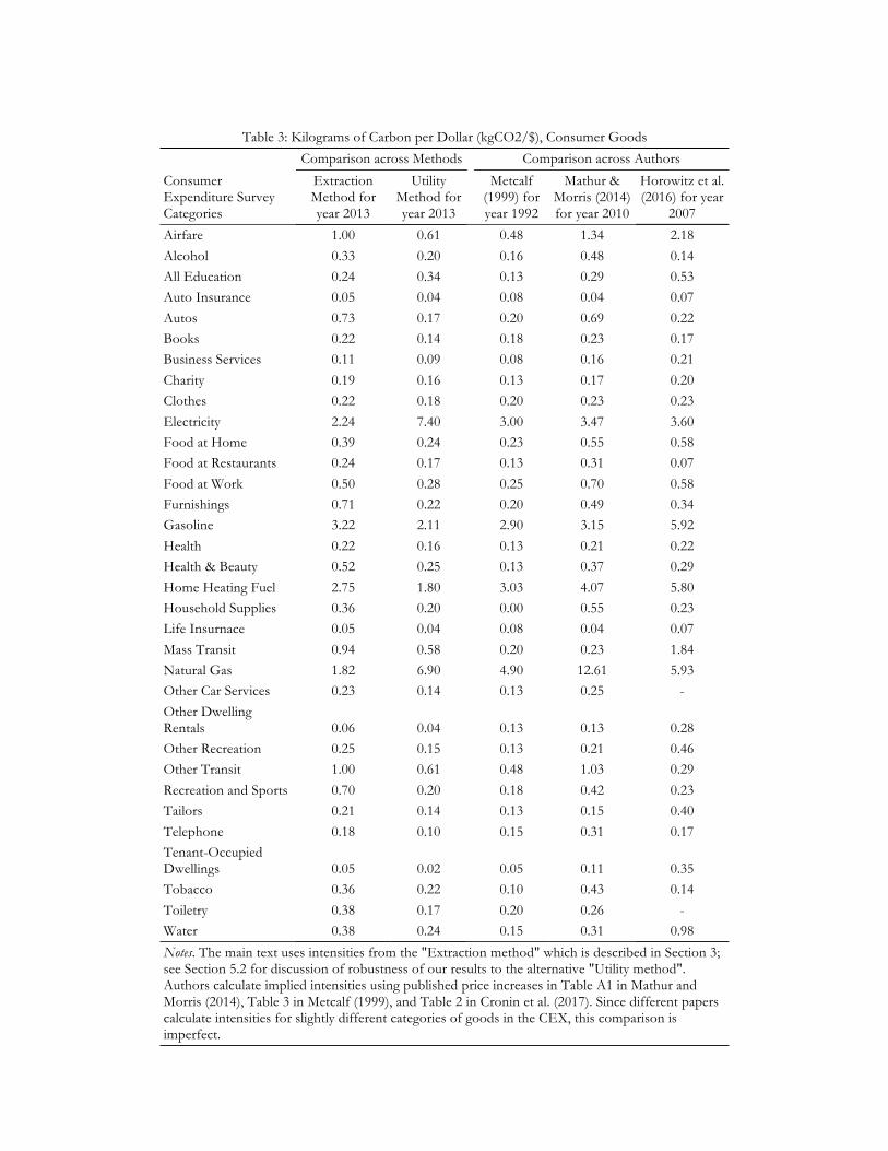
Table 3: Kilograms of Carbon per Dollar (kgCO2/$), Consumer Goods

Comparison across Methods

Comparison across Authors

Consumer Expenditure Survey Categories

Extraction Method for year 2013

Utility Method for year 2013

Metcalf (1999) for year 1992

Mathur & Morris (2014) for year 2010

Horowitz et al. (2016) for year

2007 Airfare 1.00 0.61

0.48 1.34 2.18

Alcohol 0.33 0.20

0.16 0.48 0.14 All Education 0.24 0.34

0.13 0.29 0.53

Auto Insurance 0.05 0.04

0.08 0.04 0.07 Autos 0.73 0.17

0.20 0.69 0.22

Books 0.22 0.14

0.18 0.23 0.17 Business Services 0.11 0.09

0.08 0.16 0.21

Charity 0.19 0.16

0.13 0.17 0.20 Clothes 0.22 0.18

0.20 0.23 0.23

Electricity 2.24 7.40

3.00 3.47 3.60 Food at Home 0.39 0.24

0.23 0.55 0.58

Food at Restaurants 0.24 0.17

0.13 0.31 0.07 Food at Work 0.50 0.28

0.25 0.70 0.58

Furnishings 0.71 0.22

0.20 0.49 0.34 Gasoline 3.22 2.11

2.90 3.15 5.92

Health 0.22 0.16

0.13 0.21 0.22 Health & Beauty 0.52 0.25

0.13 0.37 0.29

Home Heating Fuel 2.75 1.80

3.03 4.07 5.80 Household Supplies 0.36 0.20

0.00 0.55 0.23

Life Insurnace 0.05 0.04

0.08 0.04 0.07 Mass Transit 0.94 0.58

0.20 0.23 1.84

Natural Gas 1.82 6.90

4.90 12.61 5.93 Other Car Services 0.23 0.14

0.13 0.25 -

Other Dwelling Rentals 0.06 0.04

0.13 0.13 0.28

Other Recreation 0.25 0.15

0.13 0.21 0.46 Other Transit 1.00 0.61

0.48 1.03 0.29

Recreation and Sports 0.70 0.20

0.18 0.42 0.23 Tailors 0.21 0.14

0.13 0.15 0.40

Telephone 0.18 0.10

0.15 0.31 0.17 Tenant-Occupied Dwellings 0.05 0.02

0.05 0.11 0.35

Tobacco 0.36 0.22

0.10 0.43 0.14 Toiletry 0.38 0.17

0.20 0.26 -

Water 0.38 0.24

0.15 0.31 0.98 Notes. The main text uses intensities from the "Extraction method" which is described in Section 3; see Section 5.2 for discussion of robustness of our results to the alternative "Utility method". Authors calculate implied intensities using published price increases in Table A1 in Mathur and Morris (2014), Table 3 in Metcalf (1999), and Table 2 in Cronin et al. (2017). Since different papers calculate intensities for slightly different categories of goods in the CEX, this comparison is imperfect.

Table 4: Distribution of CO2 Emissions Across Households and Individuals

Households

Individuals

Decile by Total Household

Expenditures Household

Size

Annual Household

CO2 Emissions (kg/year)

Annual Per Capita CO2 Emissions (kg/year)

Fraction of Households Below Mean

Household CO2 Emissions

Decile by Equivalent Household

Expenditures Household

Size

Annual Household

CO2 Emissions (kg/year)

Annual Per Capita CO2 Emissions (kg/year)

Fraction of Individuals

Below Mean Per Capita CO2

Emissions 1 1.44 7,577 6,101 0.87

1 3.69 11,716 3,801 0.99

2 1.84 11,543 7,833 0.71

2 3.63 16,282 5,296 0.95 3 2.10 14,653 8,968 0.63

3 3.54 18,848 6,197 0.91

4 2.34 17,459 9,611 0.60

4 3.44 21,895 7,317 0.84 5 2.55 19,472 9,982 0.56

5 3.35 23,612 8,222 0.75

6 2.67 23,351 11,062 0.50

6 3.37 28,009 9,492 0.61 7 2.80 26,904 12,031 0.46

7 4.12 32,867 10,222 0.52

8 2.91 31,428 13,453 0.37

8 3.15 34,144 12,108 0.34 9 3.14 37,689 14,573 0.29

9 3.08 39,914 14,516 0.17

10 3.26 53,524 19,835 0.11

10 2.86 52,554 20,734 0.05 Mean 2.50 24,360 11,345 0.51

Mean 3.42 27,984 9,790 0.61

Ratio of Top and Bottom

Deciles 2.26 7.06 3.25

Ratio of Top and Bottom

Deciles 0.78 4.49 5.46

Notes. This table compares the distribution of CO2 emissions using either households or individuals as the unit of analysis. Households are sorted into deciles by household expenditures using household weights. Individuals are sorted into deciles by equivalent household expenditures using the square root scale: equivalent household expenditures = household expenditures/(household size^1/2). In the latter case, we multiply household weights by the number of people in the household to maintain the same number of people in each decile.

Table 5: Distribution of Burden of $49/Ton Tax on CO2 with Revenue Recycling

Net Transfer to Households

Fraction of Individuals Better Off

Decile by Equivalent Household

Expenditures

Equivalent Household

Expenditures

Per Capita CO2

Emissions (kg/year)

Average Cost of CO2 Tax

to Household

Cost of Tax As % of Household

Expenditures

Proportional Labor Tax

Cut

OASDI Payroll Tax Cut Dividend

Proportional Labor Tax

Cut

OASDI Payroll Tax Cut Dividend

1 $9,980 3,801 $575 3.1

-$298 -$273 $1,193

0.05 0.18 0.99 2 $14,670 5,296 $798 3.0

-$252 -$204 $944

0.16 0.29 0.95

3 $18,123 6,196 $923 2.8

-$128 -$61 $775

0.28 0.43 0.91 4 $21,564 7,317 $1,073 2.8

-$73 $0 $576

0.35 0.50 0.84

5 $25,326 8,222 $1,157 2.6

$29 $114 $449

0.42 0.54 0.75 6 $29,411 9,499 $1,373 2.6

-$65 $33 $244

0.42 0.52 0.61

7 $34,301 10,224 $1,611 2.5

$419 $502 $365

0.54 0.59 0.52 8 $40,610 12,110 $1,674 2.4

$183 $268 -$160

0.59 0.61 0.34

9 $50,784 14,516 $1,956 2.3

$504 $395 -$480

0.64 0.62 0.17 10 $79,719 20,740 $2,576 2.0

$714 $238 -$1,204

0.68 0.55 0.05

Mean Total Population $32,449 9,792 $1,372 2.6 $103 $101 $270 0.41 0.48 0.61

Mean bottom half $17,933 6,166 $905 2.9 -$145 -$85 $788 0.25 0.39 0.89

Notes. Households are sorted into deciles by equivalent household expenditures using the square root scale, where equivalent household expenditures = household expenditures/(household size^1/2). Under a $49 tax on carbon the proportional labor tax cut would increase after-tax all wages by 2.3 percent, the OASDI payroll tax cut would reduce the payroll tax rate by 2.5 percentage points, and the equal per capita dividend amounts to $479 per person.

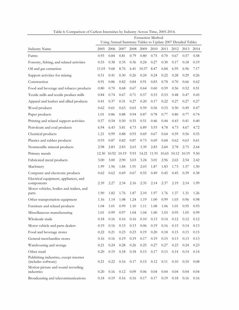
Table 6: Comparison of Carbon Intensities by Industry Across Time, 2005-2014.

Extraction Method Using Annual Summary Tables to Update 2007 Detailed Tables

Industry Name 2005 2006 2007 2008 2009 2010 2011 2012 2013 2014

Farms 0.93 0.84 0.81 0.79 0.80 0.75 0.70 0.67 0.57 0.58

Forestry, fishing, and related activities 0.55 0.38 0.35 0.36 0.24 0.27 0.30 0.17 0.18 0.19

Oil and gas extraction 11.03 9.68 8.76 6.41 10.57 8.47 6.84 6.95 6.96 7.17

Support activities for mining 0.51 0.41 0.30 0.26 0.24 0.24 0.22 0.28 0.29 0.26

Construction 0.91 0.86 0.82 0.84 0.91 0.83 0.78 0.70 0.66 0.62

Food and beverage and tobacco products 0.80 0.70 0.68 0.67 0.64 0.60 0.59 0.56 0.52 0.51

Textile mills and textile product mills 0.84 0.74 0.67 0.71 0.57 0.53 0.53 0.48 0.47 0.45

Apparel and leather and allied products 0.41 0.37 0.31 0.27 0.20 0.17 0.22 0.27 0.27 0.27

Wood products 0.62 0.61 0.63 0.65 0.59 0.56 0.53 0.50 0.49 0.47

Paper products 1.01 0.86 0.88 0.94 0.87 0.78 0.77 0.80 0.77 0.74

Printing and related support activities 0.57 0.54 0.50 0.55 0.51 0.46 0.44 0.43 0.41 0.40

Petroleum and coal products 6.94 6.43 5.81 4.73 6.89 5.93 4.78 4.73 4.67 4.72

Chemical products 1.21 0.99 0.88 0.93 0.69 0.67 0.64 0.59 0.56 0.55

Plastics and rubber products 0.93 0.87 0.82 0.87 0.73 0.69 0.68 0.62 0.63 0.61

Nonmetallic mineral products 2.98 2.83 2.83 2.63 3.39 2.83 2.60 2.78 2.75 2.64

Primary metals 12.30 10.92 10.19 9.93 14.21 11.91 10.65 10.12 10.19 9.50

Fabricated metal products 3.00 3.00 2.90 3.03 3.24 3.01 2.96 2.65 2.54 2.42

Machinery 1.99 1.96 1.84 1.91 2.03 1.87 1.83 1.73 1.57 1.50

Computer and electronic products 0.62 0.62 0.69 0.67 0.55 0.49 0.45 0.45 0.39 0.38 Electrical equipment, appliances, and components 2.39 2.27 2.34 2.16 2.35 2.14 2.37 2.19 2.14 1.99 Motor vehicles, bodies and trailers, and parts 1.90 1.82 1.76 1.87 2.10 1.97 1.76 1.37 1.31 1.26

Other transportation equipment 1.16 1.14 1.08 1.24 1.19 1.00 0.99 1.03 0.96 0.98

Furniture and related products 1.04 1.01 0.99 1.10 1.11 1.08 1.06 1.01 0.95 0.93

Miscellaneous manufacturing 1.01 0.99 0.97 1.04 1.04 1.00 1.03 0.95 1.05 0.99

Wholesale trade 0.18 0.16 0.16 0.16 0.10 0.13 0.14 0.12 0.12 0.12

Motor vehicle and parts dealers 0.19 0.16 0.15 0.13 0.06 0.19 0.16 0.15 0.14 0.13

Food and beverage stores 0.22 0.21 0.23 0.23 0.19 0.20 0.18 0.15 0.15 0.15

General merchandise stores 0.16 0.16 0.19 0.19 0.17 0.19 0.15 0.13 0.13 0.13

Warehousing and storage 0.21 0.24 0.28 0.26 0.25 0.27 0.27 0.23 0.24 0.23

Other retail 0.20 0.19 0.18 0.18 0.15 0.17 0.15 0.14 0.14 0.14 Publishing industries, except internet (includes software) 0.21 0.22 0.16 0.17 0.15 0.12 0.11 0.10 0.10 0.08 Motion picture and sound recording industries 0.20 0.16 0.12 0.09 0.06 0.04 0.04 0.04 0.04 0.04

Broadcasting and telecommunications 0.18 0.19 0.16 0.16 0.17 0.17 0.19 0.18 0.16 0.16

Data processing, internet publishing, and other information services 0.13 0.12 0.23 0.22 0.26 0.27 0.26 0.25 0.26 0.27 Federal Reserve banks, credit intermediation, and related activities 0.12 0.10 0.11 0.12 0.11 0.10 0.07 0.05 0.06 0.06 Securities, commodity contracts, and investments 0.14 0.13 0.15 0.19 0.14 0.13 0.12 0.09 0.10 0.10

Insurance carriers and related activities 0.07 0.06 0.05 0.08 0.05 0.05 0.06 0.04 0.05 0.04

Funds, trusts, and other financial vehicles 0.10 0.09 0.11 0.13 0.11 0.09 0.09 0.07 0.08 0.08 Rental and leasing services and lessors of intangible assets 0.21 0.16 0.15 0.16 0.14 0.17 0.17 0.16 0.18 0.18

Legal services 0.11 0.10 0.09 0.06 0.07 0.08 0.07 0.06 0.07 0.07 Miscellaneous professional, scientific, and technical services 0.20 0.19 0.19 0.18 0.19 0.20 0.18 0.16 0.17 0.17 Computer systems design and related services 0.10 0.09 0.08 0.09 0.08 0.09 0.08 0.07 0.07 0.06

Management of companies and enterprises 0.17 0.16 0.17 0.17 0.15 0.16 0.15 0.12 0.12 0.12

Administrative and support services 0.23 0.21 0.19 0.19 0.19 0.18 0.17 0.16 0.17 0.17 Waste management and remediation services 0.59 0.67 0.60 0.66 0.61 0.48 0.56 0.58 0.55 0.53

Educational services 0.43 0.35 0.30 0.33 0.32 0.32 0.28 0.22 0.24 0.24

Ambulatory health care services 0.23 0.20 0.18 0.19 0.17 0.17 0.15 0.14 0.14 0.13

Hospitals 0.31 0.27 0.25 0.25 0.23 0.22 0.21 0.18 0.21 0.21

Nursing and residential care facilities 0.28 0.26 0.24 0.24 0.23 0.22 0.20 0.17 0.19 0.18

Social assistance 0.27 0.25 0.24 0.26 0.26 0.27 0.25 0.20 0.19 0.18 Performing arts, spectator sports, museums, and related activities 0.18 0.16 0.17 0.17 0.17 0.17 0.16 0.14 0.14 0.13 Amusements, gambling, and recreation industries 0.28 0.28 0.27 0.28 0.31 0.28 0.28 0.24 0.25 0.23

Accommodation 0.32 0.30 0.31 0.27 0.27 0.22 0.18 0.19 0.17 0.17

Food services and drinking places 0.36 0.33 0.32 0.33 0.30 0.30 0.29 0.24 0.24 0.23

Other services, except government 0.24 0.24 0.24 0.27 0.24 0.25 0.23 0.20 0.21 0.21

Housing 0.05 0.05 0.05 0.04 0.05 0.04 0.04 0.04 0.05 0.05

Other real estate 0.58 0.57 0.48 0.50 0.50 0.51 0.38 0.29 0.32 0.31

Coal mining 92.34 80.79 72.96 64.74 86.58 69.86 60.17 66.52 67.56 63.67

Electricity utilities* 3.46 3.04 3.05 2.78 3.62 2.90 2.15 1.94 2.24 2.18

Natural gas utilities 5.14 4.01 3.75 3.24 3.65 3.01 2.08 1.53 1.82 2.08

Government 0.60 0.55 0.52 0.50 0.56 0.50 0.47 0.44 0.41 0.39

All mining except coal, oil, and gas 2.96 2.68 2.52 2.44 2.84 2.62 2.34 2.18 2.13 1.97

Transportation* 1.18 1.13 1.16 1.04 1.05 1.05 1.03 1.01 1.00 0.99

Water utilities 0.45 0.39 0.46 0.43 0.37 0.31 0.25 0.24 0.26 0.26

Notes. A (*) denotes author-generated industries in Summary Tables. Authors combine multiple industries into Government and Transportation industries.

Table 7: Distribution of Burden of $49/Ton Tax on CO2, Utility Method

Net Transfer to Household

Fraction of Individuals Better Off

Decile by Equivalent Household

Expenditures

Average Annual

Expenditure

Annual Per Capita CO2 Emissions (kg/year)

Average Annual Cost of CO2 Tax

to Household

Cost of Tax As % of Household

Expenditures

Proportional Labor Tax

Cut

OASDI Payroll Tax Cut Dividend

Proportional Labor Tax

Cut

OASDI Payroll Tax Cut Dividend

1 9,980 5795 $850 4.6

-$552 -$525 $1,053

0.07 0.09 0.92

2 14,670 7203 $1,048 3.9

-$462 -$410 $825

0.20 0.24 0.86

3 18,123 7887 $1,135 3.5

-$281 -$208 $692

0.33 0.39 0.82

4 21,564 8809 $1,261 3.3

-$187 -$108 $513

0.39 0.45 0.76

5 25,326 9579 $1,321 2.9

-$46 $46 $407

0.45 0.52 0.69

6 29,411 10543 $1,481 2.8

-$75 $31 $259

0.46 0.52 0.60

7 34,301 11020 $1,775 2.8

$408 $497 $351

0.59 0.62 0.55

8 40,610 12217 $1,664 2.4

$331 $423 -$37

0.63 0.66 0.44

9 50,784 13768 $1,847 2.1

$798 $681 -$259

0.68 0.72 0.31

10 79,719 18517 $2,296 1.8

$1,241 $729 -$821

0.70 0.68 0.09

Mean Total Population

32,449 10,534 $1,468 3.0

$118 $115 $298

0.45 0.49 0.60

Mean bottom half

17,933 7,855 $1,123 3.6

-$305 -$241 $698

0.29 0.34 0.81

Notes. Households are sorted into deciles by equivalent household expenditures using the square root scale, where equivalent household expenditures = household expenditures/(household size^1/2). Under a $49 tax on carbon the proportional labor tax cut would increase after-tax all wages by 2.5 percent, the OASDI payroll tax cut would reduce the payroll tax rate by 2.7 percentage points, and the equal per capita dividend amounts to $516 per person.

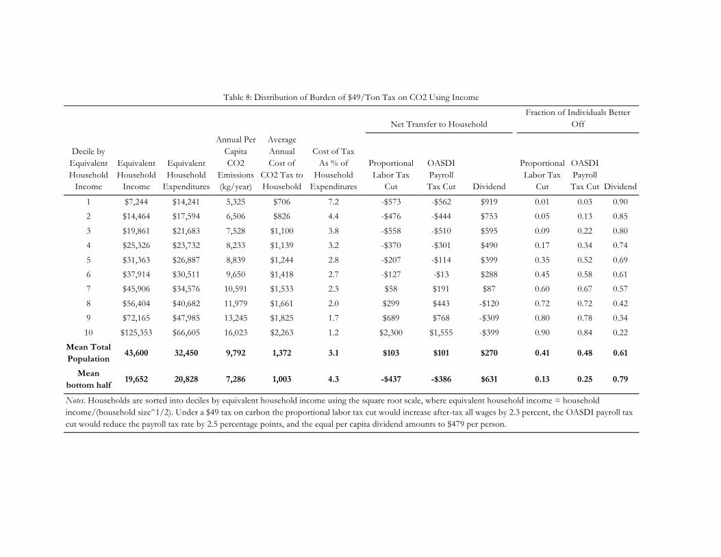
Table 8: Distribution of Burden of $49/Ton Tax on CO2 Using Income

Net Transfer to Household

Fraction of Individuals Better Off

Decile by Equivalent Household

Income

Equivalent Household

Income

Equivalent Household

Expenditures

Annual Per Capita CO2

Emissions (kg/year)

Average Annual Cost of

CO2 Tax to Household

Cost of Tax As % of

Household Expenditures

Proportional Labor Tax

Cut

OASDI Payroll Tax Cut Dividend

Proportional Labor Tax

Cut

OASDI Payroll Tax Cut Dividend

1 $7,244 $14,241 5,325 $706 7.2

-$573 -$562 $919

0.01 0.03 0.90

2 $14,464 $17,594 6,506 $826 4.4

-$476 -$444 $753

0.05 0.13 0.85

3 $19,861 $21,683 7,528 $1,100 3.8

-$558 -$510 $595

0.09 0.22 0.80

4 $25,326 $23,732 8,233 $1,139 3.2

-$370 -$301 $490

0.17 0.34 0.74

5 $31,363 $26,887 8,839 $1,244 2.8

-$207 -$114 $399

0.35 0.52 0.69

6 $37,914 $30,511 9,650 $1,418 2.7

-$127 -$13 $288

0.45 0.58 0.61

7 $45,906 $34,576 10,591 $1,533 2.3

$58 $191 $87

0.60 0.67 0.57

8 $56,404 $40,682 11,979 $1,661 2.0

$299 $443 -$120

0.72 0.72 0.42

9 $72,165 $47,985 13,245 $1,825 1.7

$689 $768 -$309

0.80 0.78 0.34

10 $125,353 $66,605 16,023 $2,263 1.2

$2,300 $1,555 -$399

0.90 0.84 0.22

Mean Total Population

43,600 32,450 9,792 1,372 3.1

$103 $101 $270

0.41 0.48 0.61

Mean bottom half

19,652 20,828 7,286 1,003 4.3

-$437 -$386 $631

0.13 0.25 0.79

Notes. Households are sorted into deciles by equivalent household income using the square root scale, where equivalent household income = household income/(household size^1/2). Under a $49 tax on carbon the proportional labor tax cut would increase after-tax all wages by 2.3 percent, the OASDI payroll tax cut would reduce the payroll tax rate by 2.5 percentage points, and the equal per capita dividend amounts to $479 per person.

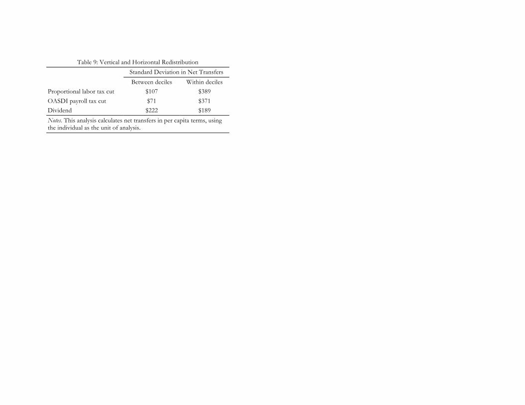
Table 9: Vertical and Horizontal Redistribution

Standard Deviation in Net Transfers

Between deciles Within deciles

Proportional labor tax cut $107 $389 OASDI payroll tax cut $71 $371 Dividend $222 $189 Notes. This analysis calculates net transfers in per capita terms, using the individual as the unit of analysis.

Table 9: Distribution of Burden of $200/Ton Tax on CO2 with Revenue Recycling

Net Transfer to Households

Fraction of Individuals Better Off

Decile by Equivalent Household

Expenditures

Equivalent Household

Expenditures

Per Capita CO2

Emissions (kg/year)

Average Cost of CO2 Tax

to Household

Cost of Tax As % of

Household Expenditures

Proportional Labor Tax

Cut

OASDI Payroll Tax Cut Dividend

Proportional Labor Tax

Cut

OASDI Payroll Tax Cut Dividend

1 $9,980 3801 $2,347 12.8

-$1,217 -$1,116 $4,871

0.01 0.03 0.90 2 $14,670 5296 $3,258 12.1

-$1,031 -$834 $3,852

0.05 0.13 0.85

3 $18,123 6196 $3,769 11.5

-$523 -$249 $3,164

0.09 0.22 0.80 4 $21,564 7317 $4,378 11.3

-$300 $0 $2,353

0.17 0.34 0.74

5 $25,326 8222 $4,723 10.5

$119 $467 $1,833

0.35 0.52 0.69 6 $29,411 9499 $5,605 10.7

-$266 $135 $998

0.45 0.58 0.61

7 $34,301 10224 $6,575 10.2

$1,712 $2,049 $1,489

0.60 0.67 0.57 8 $40,610 12110 $6,831 9.7

$746 $1,094 -$655

0.72 0.72 0.42

9 $50,784 14516 $7,983 9.2

$2,058 $1,614 -$1,960

0.80 0.78 0.34 10 $79,719 20740 $10,512 8.1

$2,914 $970 -$4,916

0.90 0.84 0.22

Mean Total Population $32,449 9,792 $5,598 10.6

$421 $413 $1,103

0.41 0.48 0.61

Mean Bottom Half $17,933 6,166 $3,695 11.6

-$590 -$346 $3,215

0.13 0.25 0.79

Notes. Households are sorted into deciles by equivalent household expenditures using the square root scale, where equivalent household expenditures = household expenditures/(household size^1/2). Under a $200 tax on carbon the proportional labor tax cut would increase after-tax all wages by 9.4 percent, the OASDI payroll tax cut would reduce the payroll tax rate by 10.2 percentage points, and the equal per capita dividend amounts to $1,958 per person.