A Discrete Theory and Efficient Algorithms for

Forward-and-Backward Diffusion Filtering

Martin WelkPrivate University for Health Sciences, Medical Informatics and Technology (UMIT)

Eduard-Wallnofer-Zentrum 16060 Hall/Tyrol, AustriaTel.: +43-50-86483974martin.welk@umit.at

Joachim WeickertMathematical Image Analysis Group

Faculty of Mathematics and Computer Science, Campus E1.7Saarland University

66041 Saarbrucken, GermanyTel.: +49-681-30257340

weickert@mia.uni-saarland.de

Guy GilboaElectrical Engineering Department

Technion – IITTechnion City, Haifa 32000, Israel

Tel.: +972-4-8294653guy.gilboa@ee.technion.ac.il

September 20, 2017

Abstract

Image enhancement with forward-and-backward (FAB) diffusion lacks a sound theoryand is numerically very challenging due to its diffusivities that are negative within acertain gradient range. In our paper we address both problems. First we establish acomprehensive theory for space-discrete and time-continuous FAB diffusion processes. Itrequires to approximate the gradient magnitude with a nonstandard discretisation. Thenwe show that this theory carries over to the fully discrete case, when an explicit timediscretisation with a fairly restrictive step size limit is applied. To come up with moreefficient algorithms we propose three accelerated schemes: (i) an explicit scheme withglobal time step size adaptation that is also well-suited for parallel implementations onGPUs, (ii) a randomised two-pixel scheme that offers optimal adaptivity of the time stepsize, (iii) a deterministic two-pixel scheme which benefits from less restrictive consistencybounds. Our experiments demonstrate that these algorithms allow speed-ups by up tothree orders of magnitude without compromising stability or introducing visual artifacts.

Keywords: image enhancement • diffusion filtering • backward parabolic PDEs • dy-namical systems • nonstandard finite differences • ill-posed problems

1

1 Introduction

Partial differential equations (PDEs) and variational approaches for enhancing digital imageshave been investigated intensively in the last thirty years. An overview can be found e.g. in[1, 33]. As continuous frameworks, these approaches excel by their concise and transparentformulation and their natural representation of rotational invariance.

However, some highly interesting models are affected by well-posedness problems, makingtheir analysis in a continuous setting difficult. Well-posedness properties of space-discreteand fully-discrete formulations therefore receive increasing attention.

Regarding the Perona–Malik filter, a space-discrete and fully discrete theory for smoothnonnegative diffusivities was established by Weickert [33]. The corresponding explicit schemewas proven in [34] to preserve monotonicity in 1D. This explains that staircasing is theworst phenomenon that can happen. An extension of this analysis to singular nonnegativediffusivities was accomplished by Pollak et al. [25] who verified the well-posedness of dynamicalsystems with discontinuous right hand sides arising from a space-discrete Perona-Malik model.

Using backward diffusion to enhance image features has a long tradition, going backalready to a 1955 publication by Kovasznay and Joseph [12] and a 1965 paper by Gabor[8, 15]. Since backward diffusion is a classical example of an ill-posed problem [29], designingappropriate numerical schemes for these processes continues to be a difficult research topic;see e.g. the recent papers [5, 6, 40] and the references therein. For the stabilised inverselinear diffusion process introduced by Osher and Rudin, a continuous well-posedness theoryis lacking, but a stable minmod discretisation could be devised [21]. Breuß and Welk [3]showed that staircasing cannot be avoided by suitable space discretisations.

For shock filtering [13, 22] which, too, is difficult to analyse in the continuous setting,discrete well-posedness results are found in [38], including an analytic solution of the corre-sponding dynamical system.

On the variational side, Nikolova has published a number of impressive papers that providedeep insights into the behaviour of minimisers of space-discrete energies, even if they are highlynonconvex or nondifferentiable; see e.g. [19, 20]. It would have been extremely difficult if notimpossible to obtain similar results in the continuous setting.

The forward-and-backward (FAB) diffusion model of Gilboa et al. [10] is another examplefor such difficulties. Designed for the sharpening of images, it is basically a Perona–Maliktype PDE filter. However, its diffusivities take positive values in some regions and negativevalues in others. Thus, it is not surprising that no well-posedness results are available in thecontinuous setting and experiments with standard explicit discretisations show violations ofa maximum–minimum principle. On the other hand, FAB diffusion has been modified andgeneralised in a number of ways [9, 26, 27, 30, 31, 32]. Thus, it would clearly be desirableto have some theoretical underpinnings and reliable and efficient algorithms for this class ofmethods. However, in view of the difficulties described above, it is most promising to establisha sound theory if one focuses on discrete FAB models.

Our Contribution. The goal of our paper is to address these two problems. In a first step,we establish a space-discrete diffusion theory that generalises the results from Weickert [33]which are only applicable for positive diffusivities. By relaxing some of its requirements weend up with a framework that can also be applied to space-discrete FAB diffusion: In partic-ular, we can establish well-posedness, a preservation of the average grey value, a maximum–

2

minimum principle, an interesting Lyapunov function and convergence to a discrete steadystate. However, these results hold only if we replace the standard discretisation of the gradientmagnitude by a nonstandard one that vanishes at discrete extrema. We show that this theoryalso carries over to the fully discrete setting with an explicit time discretisation, if the timestep size stays below a very severe bound that results from worst case a priori estimates. Byreplacing them with more realistic a posteriori estimates we end up with much more efficientschemes. They may either adapt the time step size for all locations simultaneously, or theycan be based on estimates with maximal locality / adaptivity by splitting the diffusion intopairs of neighbouring pixels. Our experiments show that these acceleration strategies canlead to speed-ups of up to three orders of magnitude.

The present paper is based on two conference publications [35, 37]: The first one haspresented early results on a space-discrete theory and one-dimensional experiments, whereasthe second one focuses on a fully discrete theory and an efficient randomised two-pixel schemefor 2D images. Our present manuscript extends these preliminary findings in several ways:

• In the space-discrete and time-continuous setting, we establish Lyapunov functions andcome up with convergence results.

• In the fully discrete framework, we propose two novel schemes:(i) An explicit scheme with global time step size adaptation and its parallelisation on aGPU.(ii) A deterministic two-pixel scheme that outperforms its randomised predecessor from[37] w.r.t. its consistency properties and its efficiency.

• Our experiments are more comprehensive and include e.g. also comparisons betweendifferent types of FAB diffusivities.

Structure of the Paper. Sections 2 and 3 provide concepts that are essential for un-derstanding the remainder of our paper by reviewing FAB diffusion [10] and the classicalspace-discrete diffusion framework from [33], respectively. In Section 4 we introduce ournovel space-discrete theory that is also applicable to FAB diffusion. A corresponding fullydiscrete theory for explicit schemes is established in Section 5. Section 6 discusses severalalgorithmic variants which are substantially more efficient by exploiting local adaptivity orparallelism, and Section 7 confirms this by experiments. The paper is concluded with asummary and an outlook in Section 8.

2 Forward-and-Backward Diffusion Filtering

Forward-and-backward (FAB) diffusion filtering has been proposed by Gilboa, Sochen andZeevi in 2002 [10]. We recall the basic definitions for the 2-D case (generalisation to arbitrarydimensions is straightforward).

The starting point is the well-known nonlinear diffusion model of Perona and Malik [24].Let a greyscale image f : Ω → R on a rectangular image domain Ω ⊂ R2 be given. To enhancethis image, filtered versions u(x, t) of f(x) are created by solving an initial–boundary valueproblem for the PDE

∂tu = div(g(|∇u|2)∇u

)(1)

3

with the input image f as initial condition,

u(x, 0) = f(x) , (2)

and homogeneous Neumann boundary conditions,

∂nu = 0 , (3)

where n denotes a vector normal to the image boundary ∂Ω . Here x stands for (x, y)>.Writing partial derivatives by subscripts, we denote by ∇ := (∂x, ∂y)> the spatial gradientand by div its corresponding divergence operator.

The specificity of FAB diffusion is the choice of the diffusivity function. The Perona–Malikframework [24] requires g to take positive values. In contrast, a FAB diffusivity is positive forsmall image gradients, while it becomes negative for larger ones. Different models for suchdiffusivities g have been proposed, see for example [9, 26]. In [9] the diffusivity

g(s2) =1√

1 + (s/kf )2− α

1 + (s/kb)2, (4)

is proposed, where kf and kb control the gradient magnitudes for forward and backwarddiffusion, respectively, and α is the weight between these terms. Note that for small imagegradients, this diffusivity is positive, while it becomes negative for larger ones, and finallybecomes positive again. Another example, adapted from [26], is

g(s2) = 2 exp

(−κ

2 ln 2

κ2 − 1· s

2

λ2

)− exp

(− ln 2

κ2 − 1· s

2

λ2

)(5)

with admissible parameters λ > 0 and κ > 1. In contrast to (4), this diffusivity does notbecome positive again for large gradient magnitudes: Asymptotically it approaches 0 frombelow when the gradient magnitude grows to infinity. We will discuss different types of FABdiffusivities in more detail in Subsection 7.4.

The main motivation for FAB was to introduce a general-purpose stable image sharpeningprocess for which dominant gradients, above the noise level, are strongly enhanced.

Like some other types of nonlinear diffusion processes, FAB diffusion can be related tovariational approaches. In [9] FAB diffusion with the diffusivity (4) has been interpreted asan energy minimisation process of a nonmonotone potential in the shape of a triple-well. FABdiffusion has also been put into relation with wavelet methods for image enhancement [18]. Aschematic form of the FAB diffusivity is shown in Figure 1. Several examples of diffusivitiesand their corresponding potentials (penalisers) are plotted within the experimental section inFigure 5.

Beyond these works, there is not much theoretical analysis of the fully continuous FABprocess documented in the literature. In particular, no existence, uniqueness and stabilityresults have been proven. In [10] it was conjectured that FAB diffusion violates a maximum–minimum principle due to the effect of negative diffusivities.

Indeed, such violations can be observed in numerical experiments, where FAB diffusion isdiscretised using standard numerical methods. However, this is no longer true if more sophis-ticated space discretisations are used: As [35] brought out, one can discretise FAB diffusionin a way such that the space-discrete process obeys the maximum–minimum principle, and

4

further useful theoretical results on the space-discrete process could be established. Stabilityproperties of fully discrete FAB diffusion were considered in [35], too, but limited to the 1Dcase. This analysis was extended to the 2D case in [37]. In Sections 4 and 5, we will alsodetail the analytical results from [35] and [37], focusing on the 2D case.

3 A Space-Discrete Diffusion Framework

Let us now review the space-discrete diffusion framework of Weickert [33], since parts of itcan be extended to the FAB setting.

To study diffusion in the space-discrete 2D case, we consider the discrete image domain

Γ := 1, 2, . . . ,m × 1, 2, . . . , n . (6)

Each pixel (i, j) ∈ Γ is assumed to be centred in the location((i− 1

2)h1, (j− 12)h2

), where h1

and h2 denote the grid size (pixel width) in x- and y-direction, respectively.

Denoting by ui,j an approximation to u in pixel (i, j) ∈ Γ , a standard discretisation of aPerona-Malik type diffusion equation

∂tu = ∂x

(g(|∇u|2) ∂xu

)+ ∂y

(g(|∇u|2) ∂yu

)(7)

in some inner pixel (i, j) yields the ordinary differential equation

dui,jdt

=1

h1

(gi+1,j + gi,j

2

ui+1,j − ui,jh1

− gi,j + gi−1,j2

ui,j − ui−1,jh1

)

+1

h2

(gi,j+1 + gi,j

2

ui,j+1 − ui,jh2

− gi,j + gi,j−12

ui,j − ui,j−1h2

). (8)

This formula even holds for boundary pixels, provided that the homogeneous Neumann bound-ary conditions (3) are implemented by mirroring boundary pixels into dummy pixels:

uk0,j := uk1,j , ukm+1,j := ukm,j , uki,0 := uki,1 , uki,n+1 := uki,n (9)

for all indices i and j. A suitable discretisation for the diffusivity g will be discussed later.

In a more compact notation, one can represent a pixel (i, j) ∈ Γ by a single index k(i, j).This leads to

dukdt

=

2∑n=1

∑l∈Nn(k)

gl + gk2h2n

(ul − uk) , (10)

where Nn(k) are the neighbours of pixel k in n-direction (boundary pixels may have lessneighbours). This can be written as a system of ordinary differential equations (ODEs):

du

dt= A(u)u , (11)

where u = (u1, . . . , uN )>, and the N ×N matrix A(u) =(ak,l(u)

)satisfies

ak,l =

gk+gl2h2

nif l ∈ Nn(k) ,

−2∑

n=1

∑l∈Nn(k)

gk+gl2h2

nif l = k ,

0 else .

(12)

5

Denoting the index set 1, ..., N by J , a space-discrete problem class (Ps) is defined inthe following way.

Let f ∈ RN . Find a function u ∈ C1([0,∞),RN ) that satisfies the initial valueproblem

du

dt= A(u)u ,

u(0) = f ,

where A = (ai,j) has the following properties:

(S1) Lipschitz-continuity of A ∈ C(RN ,RN×N ) for every bounded subset ofRN ,

(S2) symmetry: ai,j(u) = aj,i(u) ∀ i, j ∈ J, ∀u ∈ RN ,

(S3) vanishing row sums:∑

j∈J ai,j(u) = 0 ∀ i ∈ J, ∀u ∈ RN ,

(S4) nonnegative off-diagonals: ai,j(u) ≥ 0 ∀ i 6= j, ∀u ∈ RN ,

(S5) irreducibility for all u ∈ RN .

(Ps)

One should remember that a matrix A ∈ RN×N is called irreducible if for any i, j ∈ J thereexist k0,. . . ,kr ∈ J with k0 = i and kr = j such that akpkp+1 6= 0 for p = 0, . . . , r− 1. In otherwords: There is a path from pixel i to pixel j along which the diffusivities do not vanish.

Under these requirements the subsequent result is proven in [33]:

Proposition 1 (Properties of Space-Discrete Diffusion Filtering). For the space-discrete filterclass (Ps) the following statements are valid:

(a) (Well-Posedness)For every T > 0 the problem (Ps) has a unique solution u(t) ∈ C1([0, T ],RN ). Thissolution depends continuously on the initial value and the right-hand side of the ODEsystem.

(b) (Maximum–Minimum Principle)Let a := minj∈J fj and b := maxj∈J fj. Then, a ≤ ui(t) ≤ b for all i ∈ J and t ∈ [0, T ].

(c) (Average Grey Level Invariance)The average grey level µ := 1

N

∑j∈J fj is not affected by the space-discrete diffusion filter:

1N

∑j∈J uj(t) = µ for all t > 0.

(d) (Lyapunov Functions)V (t) := Φ(u(t)) :=

∑i∈J r(ui(t)) is a Lyapunov function for all r ∈ C1[a, b] with in-

creasing r′ on [a, b]: V (t) is decreasing and bounded from below by Φ(c), where c :=(µ, ..., µ)> ∈ RN .

(e) (Convergence to a Constant Steady State)limt→∞

u(t) = c.

6

The proof shows that not all of the requirements (S1)–(S5) are necessary for each ofthe theoretical results above: Requirement (S1) is needed for local well-posedness, whileproving a maximum–minimum principle requires (S3) and (S4). Local well-posedness togetherwith the maximum–minimum principle implies global well-posedness. The average grey valueinvariance is based on (S2) and (S3). The existence of Lyapunov functionals can be establishedby means of (S2)–(S4), and convergence to a constant steady state requires (S5) in additionto (S2)–(S4).

4 Analysis of Space-Discrete FAB Diffusion

We turn now to apply the results from the previous section to space-discrete FAB diffusion.Herein we follow mostly [35], adding in Subsection 4.2 new findings on Lyapunov functionsand convergence to a constant steady state.

Whereas we write down our theory focused on the 2D regular grid Γ as introduced in(6), the analysis in the previous as well as in most of this section can be generalised straight-forwardly to diffusion in arbitrary dimensions, and even to diffusion on graphs, where theimage domain J is the node set of a graph, edges connecting neighbouring nodes are weightedby distances, and intensities propagate in the diffusion process via these edges, see [7]. Forexample, by rewriting (10) as

dukdt

=∑

l∈N (k)

gl + gk2h2k,l

(ul − uk) , (13)

(and (12) accordingly) where N (k) are all neighbours of pixel k, and hk,l := h1 for horizontaland hk,l := h2 for vertical neighbours, it becomes obvious that (13) can be used verbatim alsofor diffusion on graphs, by just redefining hk,l based on the edge weights (distances).

Specific to regular grids is Subsection 4.3 where discretisations of the diffusivity are dis-cussed.

4.1 Direct Consequences from the Space-Discrete Framework

It is straightforward to verify the prerequisites (S1)–(S5) for the popular positive diffusivityfunctions, such that Proposition 1 is applicable. However, for FAB diffusion negative diffu-sivities are possible and the situation becomes much more complicated. One immediatelysees that space-discrete FAB diffusion satisfies (S1: smoothness), (S2: symmetry), and (S3:vanishing row sums). However, this just implies local well-posedness and average grey levelinvariance.

By inspecting (12) it becomes clear that (S4: nonnegative off-diagonals) and (S5: irre-ducibility) cannot be satisfied for typical FAB diffusivities: These diffusivities may vanish(which violates (S5)) and they may even become negative (violating (S4)). As a consequence,global well-posedness, a maximum–minimum principle, Lyapunov functions and convergenceto a constant steady state cannot be proven in this way.

4.2 Scale-Space Theory under Weaker Prerequisites

For the practical applicability of FAB diffusion it would be highly desirable to have at leastglobal well-posedness and a maximum–minimum principle. Is there a remedy for these prop-

7

erties? Fortunately the answer is affirmative, since (S4: nonnegative off-diagonals) can bereplaced by a less restrictive condition that only holds at extrema:

Proposition 2 (Maximum–Minimum Principle for Space-Discrete Diffusion Filtering underWeaker Conditions). Assume that a space-discrete filter satisfies only the properties (S1)–(S3)of the framework (Ps), and

(S4a) nonnegative off-diagonals at extrema:

ai,j(u) ≥ 0 for all j ∈ J with j 6= i if u has an extremum in i.

Then the well-posedness result (a), the maximum–minimum principle (b), and the averagegrey level invariance (c) of Proposition 1 are still satisfied.

Proof. Following [33], one observes that in some pixel k that is a discrete global maximum(i.e. uk ≥ uj for all j ∈ J), condition (S4a) implies that

dukdt

=∑j∈J

akj(u)uj = akk(u)uk +∑

j∈J\k

akj(u)︸ ︷︷ ︸≥0

uj︸︷︷︸≤uk

≤ uk ·∑j∈J

akj(u)(S3)= 0 . (14)

In the same way one can prove that if k is a minimum, one has duk/dt ≥ 0.

This nonenhancement behaviour in extrema is the only place where nonnegativity is re-quired in the entire proof of the maximum–minimum principle in [33]. As a consequence, themaximum–minimum principle still holds if (S4) is replaced by the weaker condition (S4a).Moreover, together with local well-posedness, global well-posedness is obtained. This com-pletes the proof.

Further adapting the conditions of the general theory in Section 3 to FAB diffusivities,we can also devise Lyapunov functions.

Proposition 3 (Lyapunov Condition for Space-Discrete Diffusion Filtering under WeakerConditions). Assume that a space-discrete filter satisfies only the properties (S1)–(S3) of theframework (Ps) and (S4a) from Proposition 2. Assume further that there is a symmetricneighbourhood relation ∼ on J such that the following two conditions are satisfied:

(S4b) positive off-diagonals in neighbourhood of extrema:

If u has an extremum in i, ai,j(u) > 0 holds for all j ∈ J \ i with i ∼ j.(S5a) irreducibility of neighbourhood relation:

The neighbourhood graph in J based on the neighbourhood relation ∼ is con-nected.

Using umax := maxjuj, umin := min

juj and

Φ(u) := umax − umin , (15)

define then the function V : [0,∞)→ R+0 by V := Φ u, i.e.

V (t) := umax(t)− umin(t) . (16)

8

Then the Lyapunov property (d) and steady state property (e) of Proposition 1 are satisfiedwith the Lyapunov function V (t).

The proof of this proposition relies on the following statement.

Lemma 1. Under the assumptions of Proposition 3, the functions Φ and V satisfy the fol-lowing three conditions:

(i) Φ is continuous on [a, b]N , where a and b are the minimum and maximum of u0, respec-tively.

(ii) V is continuous, bounded and piecewise differentiable.

(iii) Let V ′+(t) denote the right-sided derivative of V . Then V (t) > 0 and V ′+(t) ≤ 0 hold forall t ≥ 0, with V ′+(t) = 0 only for discrete times t, unless the image f is flat.

Proof of the Lemma. Continuity of Φ w.r.t. u, and of u w.r.t. t, is straightforward, as (Ps)with the modified condition set (S1)–(S3), (S4a), (S4b), (S5a) is a dynamical system withbounded right-hand side. By concatenation, V (t) is continuous, too. By the Lipschitz-continuity of A the right-hand side of the dynamical system is even continuous, ensuringcontinuous differentiability of u(t). Therefore V is also differentiable, except at those timest when the global maximum, or minimum, of u(t) is attained by two equal-valued pixelsui(t) and uj(t) with ui(t) 6= uj(t), such that the global maximum or minimum property istransferred from one to the other pixel at time t. As the number N of pixels is finite, this canhappen only at discrete times t, and at each of these times the pixels representing the globalmaximum and minimum in the subsequent time interval establish a well-defined right-sidedderivative of V . This completes the proof of (i).

Next we prove that for a non-trivial image V ′+(t) = 0 cannot stay true throughout a timeinterval [t1, t2], t1 < t2.

For any pixel ui(t) representing the global maximum or minimum at time t, the weightsai,j(t) for all neighbours j of i are positive by hypothesis (S4b), while ai,i(t) is positive by(S4a) and (S3). Thus, ui,j = 0 can hold only if all neighbours of ui,j have the same grey valueas ui,j at time t.

Assume ui(t) is a global maximum with ui(t) = 0 throughout [t1, t2]. Then all neighbourpixels uj with j ∼ i satisfy uj = ui throughout [t1, t2], thus also uj = 0. As the image domainJ is irreducible (connected by the neighbourhood relation) by (S5), this implies by recursiveapplication that the image is a steady state. By reversibility of the dynamical system underconsideration, this is possible only if f is trivial.

Thus, V ′+(t) can vanish only at discrete time points. For all other times, V ′+(t) is negativebecause of the negative matrix entries ai,i and nonnegative ai,j for j 6= i at extrema i ∈ J .

Finally, the reversibility of the aforementioned dynamical system also ensures V (t) > 0for all times if f is nontrivial.

Proof of Proposition 3. Since the quantity Φ(u) is nonnegative, and vanishes exactly for thesteady states u(t) = c, Lemma 1 characterises V as a Lyapunov function for semidiscreteFAB diffusion on each interval [t0,∞) with t0 > 0.

The convergence result (e) will follow now by slight adaptation of a standard proof fromthe theory of dynamical systems. Note that properties (ii) and (iii) from Lemma 1 but with

9

the stronger inequality V ′(t) < 0 for all t, are a standard argument about global asymptoticstability of dynamical systems; see e.g. [23, p. 127, Theorem 3]. However, the sole purpose ofV ′ < 0 in the proof of the result is to ensure that V (t) is strictly decreasing. The latter canequally be inferred from the slightly weaker property in Lemma 1(iii). With this modification,the proof from [23] carries over.

4.3 A Nonstandard Space Discretisation for FAB Diffusion

While the preceding results are encouraging, and the standard pixel grid obviously induces aneighbourhood relation ∼ that satisfies condition (S5a), we have not yet shown that a suitablespace-discretisation satisfies the modified requirements (S4a) and (S4b) at extrema. Unfor-tunately, this issue is a bit more delicate than one might assume: A standard discretisationof the diffusivity g

(|∇u|2) in some pixel (i, j) of a regular grid Γ is given by the central

difference approximation

gi,j := g

((ui+1,j − ui−1,j

2h1

)2

+

(ui,j+1 − ui,j−1

2h2

)2). (17)

However, even if u has an extremum in (i, j), the approximation (17) of |∇u|2 may becomepositive – and not 0 as one would expect from the continuous theory. Since the FAB diffu-sivities only guarantee that g(0) > 0, it can happen that this finite difference approximationcreates negative diffusivities in extrema and (S4a) is violated.

Fortunately there is an interesting alternative to the standard discretisation of the diffu-sivity on a regular grid that solves these problems immediately. As a prerequisite, let us firstprecise our requirements for FAB diffusivities.

Definition 1 (Admissible FAB diffusivity). Let g : R+0 → R be a Lipschitz-continuous

function. Assume that there are two constants c1 > c2 > 0 such that g(0) = c1, andg(z) > −c2 for all z > 0, compare Figure 1. Then g is called admissible FAB diffusivity.

Proposition 4 (Properties of Space-Discrete FAB Diffusion). Let an admissible FAB diffu-sivity g according to Definition 1 be given. Then the space discretisation (8) of FAB diffusionis well-posed, satisfies a maximum–minimum principle and average grey level invariance, ifthe diffusivity is evaluated by the nonstandard finite difference approximation

gi,j := g

(max

(ui+1,j − ui,j

h1· ui,j − ui−1,j

h1, 0

)

+ max

(ui,j+1 − ui,j

h2· ui,j − ui,j−1

h2, 0

)). (18)

Under these conditions, the FAB evolution also satisfies the Lyapunov property with the Lya-punov function V (t) = umax(t) − umin(t), and converges to the trivial steady state u = c fort→∞.

It should be noted that this approximation has the same quadratic order of consistencyas the previous one. However, it guarantees a vanishing discrete gradient approximation inextrema. Since according to the conditions of Definition 1 the diffusivity g(0) = c1 at an

10

extremum yields a positive average with any other value of the diffusivity g, (S4a) and (S4b)are guaranteed. Interestingly, the Lipschitz continuity of g and the property g(0) > − inf

z>0g(z)

are the only requirements that are necessary to establish well-posedness, maximum–minimumprinciple, Lyapunov property and convergence to the trivial steady state for space-discreteFAB diffusion.

Nonstandard finite difference approximations that approximate nonlinear expressions bya combination of forward and backward differences have been advocated by Mickens [17] asan appropriate tool to design algorithms which capture essential physical properties of theirunderlying differential equations. Our paper confirms this.

Last but not least, our results are not restricted to the two-dimensional case: With asimilar nonstandard approximation, it is straightforward to verify that space-discrete FABdiffusion is well-posed and satisfies an extremum principle on regular grids in any dimension.

5 Analysis of Fully Discrete FAB Diffusion in 2D

Combining the spatial discretisation from Section 4 with a forward difference discretisationin time, we obtain a simple explicit scheme for (1) with time step size τ and grid sizes h1 andh2 in x- and y-direction:

uk+1i,j = uki,j + τ ·

(gki+1,j + gki,j

2·uki+1,j − uki,j

h21−gki,j + gki−1,j

2·uki,j − uki−1,j

h21

+gki,j+1 + gki,j

2·uki,j+1 − uki,j

h22−gki,j + gki,j−1

2·uki,j − uki,j−1

h22

). (19)

Here, uki,j approximates u at the grid location of (i, j) ∈ Γ and time kτ . Furthermore,we use the nonstandard approximation (18) for the admissible FAB diffusivity, computingdiffusivities gki,j in all pixels in time step k from the values uki,j in the same time step.

Our requirements to the discrete FAB diffusion problem and the diffusivity function aresummarised in the following definition.

Definition 2 (Discrete FAB evolution). Let an initial 2D image f = (fi,j) on Γ =1, 2, . . . ,m × 1, 2, . . . , n be given. Let the grey values fi,j be restricted to a finite in-terval [a, b] of length R := b− a.

The discrete FAB evolution is the sequence of images uk = (uki,j) that evolves according to

(19), (18) with the initial condition u0 = f , mirroring boundary conditions, and an admissibleFAB diffusivity function g as specified in Definition 1.

The stabilisation range constant of g is the largest constant ω = ω(g) > 0 such thatg(s2) > c2 holds for all s with 0 < s < ωR (such an ω exists due to the continuity of g;compare Figure 1).

5.1 Maximum–Minimum Principle

Our first result is a 2D analogue for the first statement of [35, Prop. 4], i.e. the maximum–minimum principle. Our bound for τ is adapted to the 2D grid geometry.

11

g(s2)

s

c1

c2

0

−c2

ωR

Figure 1: Schematic view of an admissible FAB diffusivity satisfying the conditions of Propo-sition 5.

Proposition 5 (Maximum–Minimum Principle for Discrete FAB Diffusion). Consider thediscrete FAB evolution as specified in Definition 2. Let the time step τ satisfy the inequality

τ ≤ ϑ :=ω2h41h

42

2c1(h21 + h22)(ω2h21h

22 + h21 + h22)

. (20)

Then u obeys the following maximum–minimum principle: If the initial signal is boundedby fi,j ∈ [a, b] for all (i, j) ∈ Γ , then uki,j ∈ [a, b] for all (i, j) ∈ Γ , k ≥ 0.

The proof of this statement relies on two local properties.

Lemma 2. Under the assumptions of Proposition 5, local maxima do not increase.

Proof. Let uki,j be a local maximum of uk. Then gki,j = c1, and we have that gki+1,j + gki,j etc.

are positive while uki+1,j − uki,j etc. are negative such that all summands in the bracket on ther.h.s. of (19) are negative. This holds independent of τ .

The r.h.s. of (19) is a convex combination of uki,j , uki±1,j , u

ki,j±1 if

1− τ

2h21

(gki+1,j + 2gki,j + gki−1,j

)− τ

2h22

(gki,j+1 + 2gki,j + gki,j−1

)≥ 0 , (21)

which is certainly the case if

τ ≤ 1

2 c1

(1h21

+ 1h22

) . (22)

Note that this is the well-known time step limit for the standard explicit scheme in the caseof nonnegative diffusivity. As the bound in (22) is greater than ϑ in Proposition 5, thiscompletes the proof.

Nonenhancement of local extrema is a frequently used scale-space property for linear andnonlinear diffusion processes; see e.g. [2, 14, 33]. However, in the case of FAB diffusion, weneed one more property to prove a maximum–minimum principle:

Lemma 3. Under the assumptions of Proposition 5, a non-maximal pixel does not grow inexcess of its greatest adjacent pixel within one time step.

12

Proof. Let uki,j be the non-maximal pixel under consideration. Assume first that the largest

grey value among its neighbours is attained by a horizontal neighbour, say uki−1,j . So uki−1,jis greater than uki,j and not less than each other neighbour of uki,j .

To outline the proof first, notice that basically two situations can happen: If uki,j is only

slightly smaller than uki−1,j , it turns out that uki,j is “not far from maximality”. In this case,

its diffusivity gki,j will be positive and large enough to ensure forward diffusion (Case 1 in thefollowing), such that again the time step limit of explicit forward diffusion applies. Otherwise,negative diffusivity may occur, but at the same time there is quite some way to go beforeuk+1i,j could exceed uki−1,j . The overall bounds on the image contrast limit the diffusion flow

and thereby the “speed” of the pixel. So one can state also in this case a time step size limitthat ensures the desired inequality (Case 2). In the following, these two cases are treatedexactly.

Case 1: Assume that one has

1

h21(uki,j − uki−1,j)(uki+1,j − uki,j) +

1

h22(uki,j − uki,j−1)(uki,j+1 − uki,j) ≤ ω2R2 . (23)

Then gki,j ≥ c2, and thus gki,j + gki+1,j , gki,j + gki,j±1 ≥ 0. As a consequence, uk+1

i,j is a convex

combination of uki,j , uki±1,j , u

ki,j±1 if

1− τ

2h21(gki+1,j + 2gki,j + gki−1,j)−

τ

2h22(gki,j+1 + 2gki,j + gki,j−1) ≥ 0 , (24)

which is certainly fulfilled if

1− 4τc12h21

− 4τc12h22

≥ 0 , (25)

i.e. (22).

Case 2: Let

1

h21(uki,j − uki−1,j)(uki+1,j − uki,j) +

1

h22(uki,j − uki,j−1)(uki,j+1 − uki,j) > ω2R2 . (26)

The difference between pixel uki,j and its greatest neighbour fulfils the inequality

uki−1,j − uki,j >ω2R

1h21

+ 1h22

, (27)

because the contrary would imply the hypothesis of Case 1. Further, we have by the hypothesisof Case 2 that −c2 ≤ gki,j ≤ c2. Together with the hypotheses from Proposition 5 on the rangeof g and the image range, one has

−c2 ≤gki+1,j + gki,j

2≤ c1 + c2

2, − R

h21≤uki+1,j − uki,j

h21≤ R

h21,

−c2 ≤gki−1,j + gki,j

2≤ c1 + c2

2, 0 ≤

uki−1,j − uki,jh21

≤ R

h21, (28)

13

−c2 <gki,j±1 + gki,j

2≤ c1 + c2

2, − R

h22≤uki,j±1 − uki,j

h22≤uki−1,j − uki,j

h22.

Inserting these into (19) gives

uk+1i,j ≤ u

ki,j + τ

(c1 + c2

2h21R+

c1 + c22h21

(uki−1,j − uki,j) + 2c1 + c2

2h22R

), (29)

uki−1,j − uk+1i,j ≥ (uki−1,j − uki,j)

(1− τ(c1 + c2)

2h21

)− τ(c1 + c2)R

2

(1

h21+

2

h22

). (30)

The r.h.s. of (30) is certainly nonnegative if

τ ≤ 2h21c1 + c2

·uki−1,j − uki,j

uki−1,j − uki,j +R(1 + 2h21/h

22

) , (31)

for which by our initial estimate for uki−1,j − uki,j and monotonicity it suffices that

τ ≤ 2ω2h41h42

(c1 + c2)(ω2h21h

42 + (h22 + 2h21)(h

21 + h22)

) . (32)

This limit on τ ensures that the pixel under consideration cannot grow in excess of itsgreatest neighbour if this neighbour is a horizontal neighbour. If uki,j has its greatest neighbourin vertical direction, analogous considerations lead to a similar constraint, with h1 and h2exchanged. Both bounds on τ are larger than the bound (20) of Proposition 5.

Proof of Proposition 5. The maximum–minimum principle follows immediately from Lemmas2 and 3 and analogous statements for local minima.

Remark 1. Unlike in the 1D case [35, Prop. 4], the statement that an extremum may not splitinto two does not hold. Similar to ordinary homogeneous diffusion, a “dumbbell” configurationwith a narrow ridge between two more extended plateaus can serve as a counterexample; seee.g. [14]. Note that for sufficiently small grey value differences between the ridge and theadjacent plateaus all diffusivities in this region are positive.

5.2 Strict Lyapunov Condition

The maximum–minimum principle from Proposition 5 suggests the use of the difference be-tween global maximum and global minimum of the image as a Lyapunov function to in-vestigate the possible convergence of discrete FAB diffusion. Our proofs from the previoussubsection, however, still leave the possibility that the global maximum and minimum of theimage stay constant, and different from each other, forever.

To rule out this possibility, we will refine our analysis and construct a strictly decreas-ing Lyapunov function by incorporating multiplicities of maxima and minima as additionalinformation. From now on, we require that τ is strictly smaller than the bound (20) fromProposition 5. We introduce notations for the global extremal grey values of images withtheir multiplicities, and an ordering for pairs of values with multiplicities.

Definition 3. For any image u = (ui,j)(i,j)∈Γ , let umax := maxi,j

ui,j , umin := mini,j

ui,j denote

its maximal and minimal grey value, respectively, and nmax := #(i, j) | ui,j = umax,nmin := #(i, j) | ui,j = umin their multiplicities.

14

Definition 4. Let the relation ≺ on R× N be given by

(u1, n1) ≺ (u2, n2) :⇐⇒ (u1 < u2) or (u1 = u2 and n1 < n2) . (33)

Clearly, ≺ is a strict total order. We can now establish the maximum–minimum differencewith multiplicities as Lyapunov function for discrete FAB diffusion.

Proposition 6 (Lyapunov Function for Discrete FAB Diffusion). Consider the fully discreteFAB evolution from Definition 2. If the time step size is chosen as τ < ϑ with ϑ as inProposition 5, then

(uk+1max − uk+1

min , nk+1max + nk+1

min ) ≺ (ukmax − ukmin, nkmax + nkmin) (34)

holds, unless ukmax = ukmin.

Proof. Let uki,j be a local maximum of uk. As in the proof of Lemma 2, we have gki,j = c1.

Thus, the new value uk+1i,j of that pixel will be a convex combination of the old grey values

of pixel (i, j) and its neighbours, with all neighbours having positive weights. Therefore,uk+1i,j = uki,j can happen only if all neighbours have the same value as ui,j in time step k.

As long as not all pixels of the image have the same value, there will be at least one pixeluki,j = ukmax with a neighbour of smaller grey value.

Following the proof of Lemma 3 we see that for τ < ϑ the new pixel value uk+1i,j remains

strictly below the old value of its largest neighbour uki−1,j . Thus, uk+1i,j = ukmax cannot hold

for a pixel with uki,j < ukmax.

Combining both arguments, we see that the number of pixels attaining the value ukmax

decreases in time step k + 1. As a consequence, one has uk+1max < ukmax (if no pixel with that

value remains), or nk+1max < nkmax (if the maximal value remains equal).

Analogous reasoning for minima completes the proof.

5.3 Convergence to a Flat Steady State

An immediate consequence of Proposition 6 is the following statement.

Corollary 1 (Steady States of Discrete FAB Diffusion). The only fixed points of the discreteFAB diffusion process (19), (18) are the flat images given for each µ ∈ R by

ui,j = µ for all (i, j) ∈ Γ . (35)

By average grey value invariance, the only steady state that could be reached from a giveninitial image f is that for which

µ =1

N

∑(i,j)∈Γ

fi,j , N := mn (36)

is the average grey value of f . We will now prove convergence to this steady state.

Proposition 7 (Convergence of Discrete FAB Diffusion). Fully discrete FAB diffusion (19),(18) with u0 = f and time step size τ < ϑ converges to the fixed point (35) where µ is theaverage grey value of f .

15

Proof. Consider the strictly decreasing (w.r.t. ≺) sequences((ukmax, n

kmax)

)k∈N and(

(−ukmin, nkmin)

)k∈N from Proposition 6. These sequences are bounded from below by (fmin, N)

and (−fmax, N), respectively. By an easy adaptation of the standard argument for sequencesin R to sequences in R× N it follows that the sequences (ukmax), (ukmin) converge. Denote byu, u their respective limits.

Assume u < u. By the maximum–minimum principle, uk ∈ [a, b]N holds for all k. Since[a, b]N is compact, the sequence (uk) has a cumulation point. Because of the monotonicity of(ukmax), (ukmin) each cumulation point satisfies u∗max = u, u∗min = u.

We choose one cumulation point u∗ and consider the FAB evolution (uk)k∈N0 with initialcondition u0 = u∗. By Proposition 6, there exists a natural number K such that uKmax =max u < u. Let therefore δ := u− uKmax > 0.

Moreover, the evolution (19), (18) satisfies a Lipschitz condition on [a, b]N with respectto the maximum norm ‖ · ‖, i.e.

‖uk − uk‖ < B ⇒ ‖uk+1 − uk+1‖ < LB (37)

with some Lipschitz constant L > 0. Since u∗ is a cumulation point of (uk), we can choose ksuch that ‖uk−u∗‖ < δ/LK . Consequently, ‖uk+K− uK‖ < δ, and by the triangle inequalityit follows that

uk+Kmax ≤ uKmax + ‖uk+K − uK‖ < u− δ + δ = u , (38)

contradicting the convergence of (ukmax) to u. Thus, our assumption u < u must be wrong,and we have u = u, i.e. convergence to a flat steady state.

6 Efficient Numerics for FAB Diffusion

Based on the stability result from Proposition 5 it is possible to compute FAB diffusion by astable explicit scheme. The limit (20) on the time step size, however, leads to time step sizesthat are much too small for most practical application.

In fact, (20) is an a priori estimate for the time step size which is obtained by thecombination of several worst-case estimates in the proofs in Subsection 5.1. It is very commonfor this kind of estimates that the worst-case estimates involved will in general be reachedonly at a few pixel locations within a larger image, and also rarely apply simultaneously.Indeed, in practical computation one notices that even with drastically larger time step sizes,violations of the maximum–minimum principle occur only in some time steps, affect only afew pixels, and the bounds are exceeded only by small amounts.

This motivates us to devise explicit schemes for FAB diffusion with adaptive step-sizecontrol based on a posteriori estimates of the time step size.

6.1 A Stable Explicit Scheme with Global Step Size Adaptation

We start by equipping the explicit scheme (19), (18) with a step-size control that provides ineach iteration for a global time step τ which prevents violations of stability. Our theory fromSection 5 already contains the blueprint for such a step-size control, as the criteria formulatedin Lemma 2 and Lemma 3 can immediately be used to obtain the desired a posteriori estimate.

16

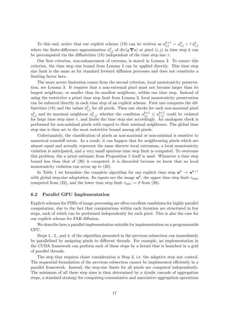
To this end, notice that our explicit scheme (19) can be written as uk+1i,j = uki,j + τ uki,j

where the finite-difference approximation uki,j of div(g∇u) at pixel (i, j) in time step k canbe precomputed via the diffusivities (18) independent of the time step size τ .

Our first criterion, non-enhancement of extrema, is stated in Lemma 2. To ensure thiscriterion, the time step size bound from Lemma 2 can be applied directly. This time stepsize limit is the same as for standard forward diffusion processes and does not constitute alimiting factor here.

The more severe limitation comes from the second criterion, local monotonicity preserva-tion, see Lemma 3. It requires that a non-extremal pixel must not become larger than itslargest neighbour, or smaller than its smallest neighbour, within one time step. Instead ofusing the restrictive a priori time step limit from Lemma 3, local monotonicity preservationcan be enforced directly in each time step of an explicit scheme. First one computes the dif-fusivities (18) and the values uki,j for all pixels. Then one checks for each non-maximal pixel

uki,j and its maximal neighbour uki′,j′ whether the condition uk+1i,j ≤ uk+1

i′,j′ could be violatedfor large time step sizes τ , and limits the time step size accordingly. An analogous check isperformed for non-minimal pixels with regard to their minimal neighbours. The global timestep size is then set to the most restrictive bound among all pixels.

Unfortunately, the classification of pixels as non-maximal or non-minimal is sensitive tonumerical roundoff errors. As a result, it can happen that for neighbouring pixels which arealmost equal and actually represent the same discrete local extremum, a local monotonicityviolation is anticipated, and a very small spurious time step limit is computed. To overcomethis problem, the a priori estimate from Proposition 5 itself is used: Whenever a time stepbound less than that of (20) is computed, it is discarded because we know that no localmonotonicity violation can occur up to (20).

In Table 1 we formulate the complete algorithm for one explicit time step uk → uk+1

with global step-size adaptation. Its inputs are the image uk, the upper time step limit τmax

computed from (22), and the lower time step limit τmin := ϑ from (20).

6.2 Parallel GPU Implementation

Explicit schemes for PDEs of image processing are often excellent candidates for highly parallelcomputation, due to the fact that computations within each iteration are structured in fewsteps, each of which can be performed independently for each pixel. This is also the case forour explicit scheme for FAB diffusion.

We describe here a parallel implementation suitable for implementation on a programmableGPU.

Steps 1., 2., and 4. of the algorithm presented in the previous subsection can immediatelybe parallelised by assigning pixels to different threads. For example, an implementation inthe CUDA framework can perform each of these steps by a kernel that is launched in a gridof parallel threads.

The step that requires closer consideration is Step 3, i.e. the adaptive step size control.The sequential formulation of the previous subsection cannot be implemented efficiently in aparallel framework. Instead, the step-size limits for all pixels are computed independently.The minimum of all these step sizes is then determined by a dyadic cascade of aggregationsteps, a standard strategy for computing commutative and associative aggregation operations

17

Table 1: Time step of explicit scheme for FAB diffusion with global adaptive step size control

Input: uk, τmax, τmin

1. Diffusivity computation: For each pixel (i, j), compute the diffusivity gi,jaccording to (18):

gki,j := g

(max

(uki+1,j − uki,j

h1·uki,j − uki−1,j

h1, 0

)

+ max

(uki,j+1 − uki,j

h2·uki,j − uki,j−1

h2, 0

)).

2. Flow computation: For each pixel (i, j), compute the right-hand side uki,j via(19):

uki,j =gki+1,j + gki,j

2·uki+1,j − uki,j

h21−gki,j + gki−1,j

2·uki,j − uki−1,j

h21

+gki,j+1 + gki,j

2·uki,j+1 − uki,j

h22−gki,j + gki,j−1

2·uki,j − uki,j−1

h22.

3. Step-size determination: Let τ := τmax.

For each pixel (i, j),

• If (i, j) is not a discrete local maximum, let (i′, j′) be its maximal neighbour.

If uki,j + τ uki,j > uki′,j′ + τ uki′,j′ , set τ∗ := −uki′,j′ − uki,juki′,j′ − uki,j

.

If τ∗ ≥ τmin, let τ = τ∗.

• If (i, j) is not a discrete local minimum, let (i′, j′) be its minimal neighbour.

If uki,j + τ uki,j < uki′,j′ + τ uki′,j′ , set τ∗ := −uki′,j′ − uki,juki′,j′ − uki,j

.

If τ∗ ≥ τmin, let τ = τ∗.

4. Global update: For each pixel (i, j), compute uk+1i,j := uki,j + τ uki,j .

18

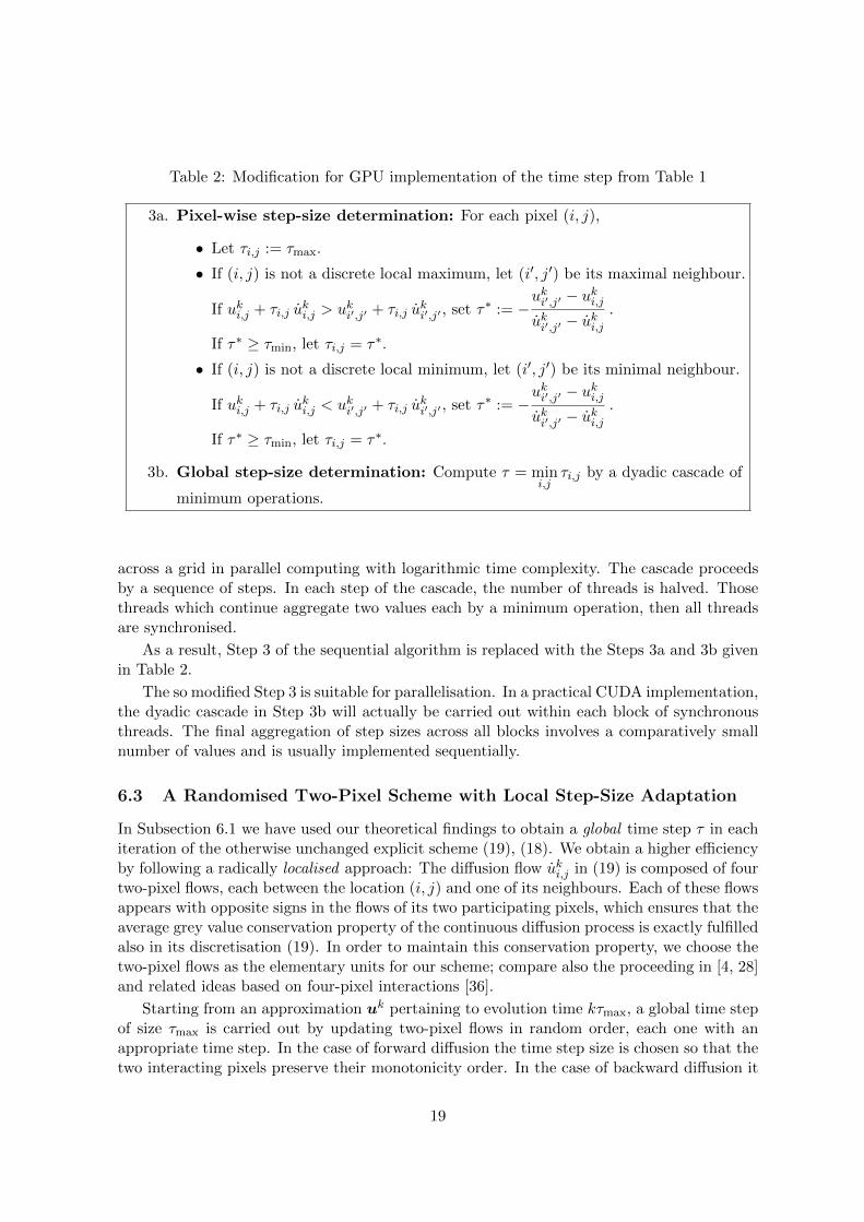
Table 2: Modification for GPU implementation of the time step from Table 1

3a. Pixel-wise step-size determination: For each pixel (i, j),

• Let τi,j := τmax.

• If (i, j) is not a discrete local maximum, let (i′, j′) be its maximal neighbour.

If uki,j + τi,j uki,j > uki′,j′ + τi,j u

ki′,j′ , set τ∗ := −

uki′,j′ − uki,juki′,j′ − uki,j

.

If τ∗ ≥ τmin, let τi,j = τ∗.

• If (i, j) is not a discrete local minimum, let (i′, j′) be its minimal neighbour.

If uki,j + τi,j uki,j < uki′,j′ + τi,j u

ki′,j′ , set τ∗ := −

uki′,j′ − uki,juki′,j′ − uki,j

.

If τ∗ ≥ τmin, let τi,j = τ∗.

3b. Global step-size determination: Compute τ = mini,j

τi,j by a dyadic cascade of

minimum operations.

across a grid in parallel computing with logarithmic time complexity. The cascade proceedsby a sequence of steps. In each step of the cascade, the number of threads is halved. Thosethreads which continue aggregate two values each by a minimum operation, then all threadsare synchronised.

As a result, Step 3 of the sequential algorithm is replaced with the Steps 3a and 3b givenin Table 2.

The so modified Step 3 is suitable for parallelisation. In a practical CUDA implementation,the dyadic cascade in Step 3b will actually be carried out within each block of synchronousthreads. The final aggregation of step sizes across all blocks involves a comparatively smallnumber of values and is usually implemented sequentially.

6.3 A Randomised Two-Pixel Scheme with Local Step-Size Adaptation

In Subsection 6.1 we have used our theoretical findings to obtain a global time step τ in eachiteration of the otherwise unchanged explicit scheme (19), (18). We obtain a higher efficiencyby following a radically localised approach: The diffusion flow uki,j in (19) is composed of fourtwo-pixel flows, each between the location (i, j) and one of its neighbours. Each of these flowsappears with opposite signs in the flows of its two participating pixels, which ensures that theaverage grey value conservation property of the continuous diffusion process is exactly fulfilledalso in its discretisation (19). In order to maintain this conservation property, we choose thetwo-pixel flows as the elementary units for our scheme; compare also the proceeding in [4, 28]and related ideas based on four-pixel interactions [36].

Starting from an approximation uk pertaining to evolution time kτmax, a global time stepof size τmax is carried out by updating two-pixel flows in random order, each one with anappropriate time step. In the case of forward diffusion the time step size is chosen so that thetwo interacting pixels preserve their monotonicity order. In the case of backward diffusion it

19

is chosen such that they are prevented from growing above the maximum, or decreasing belowthe minimum of their respective neighbourhoods. Updated values ui,j enter immediately thecomputation of other pixels. This is repeated until all flows have reached the new time level,yielding the new approximation uk+1.

The time step k 7→ k + 1 is summarised in Table 3. It starts by initialising an evolutiontime account for each pair of neighbouring pixels with τmax. Then pixel pairs are randomlyselected and updated until all time accounts reach zero, indicating that we have progressedfrom sync time kτmax to (k + 1)τmax.

This process terminates, since τ∗ cannot fall below the global positive limit ϑ from (20).

6.3.1 Consistency of the Scheme

Our scheme is conditionally consistent. To understand this, let us assume for simplicityh1 = h2 = h. The forward difference approximation in t and central difference approxima-tions in the spatial domain generate approximation errors of O(τ+h2) as for conventional ex-plicit schemes. Additional approximation errors result from the asynchronous update process.When computing a two-pixel flow u = g ·(ui′,j′−ui,j)/h2, the value ui,j is the sum of uki,j fromthe previous synchronisation time and several independent updates of the flows between (i, j)and its neighbours. Thus, ui,j carries an approximation error of O(ux ·τ/h+uy ·τ/h); similarlyfor ui′,j′ . Each two-pixel flow therefore incurs an approximation error due to asynchronicityof O(τ/h3), making the overall approximation error of our scheme O(τ + h2 + τ/h3). Thisyields a conditionally consistent approximation to the FAB diffusion PDE if τ/h4 is boundedby a constant when τ, h→ 0.

On the other hand, sending the grid size h to 0 is not necessarily what one does in typicalimage processing applications. If one keeps the grid size constant and is only interested inthe limit τ → 0, our randomised two-pixel scheme gives an O(τ) approximation to the space-discrete FAB process. In that respect, it has the same consistency quality as the explicitscheme.

6.3.2 Efficient Random Selection and Time Accounting

For an efficient implementation of the algorithm, the performance of the selection in Step 1is crucial. To this end, the bookkeeping of time step accounts Ti,j;i′,j′ is done within a binarytree structure as follows.

Data Structure. Let M = (m − 1)n + m(n − 1) be the number of pairs (i, j), (i′, j′) ofneighbouring pixels. Let P = 2p be the smallest power of two greater than M . We index pixelpairs by indices ` ∈ 0, . . . ,M − 1 from which the corresponding i, j, i′, j′ can be computedin constant computation time as follows:

• If ` < (m− 1)n, create a horizontal neighbour pair by

i :=

⌊`

n

⌋+ 1 ∈ 1, . . . ,m− 1 ,

j := `− n(i− 1) + 1 ∈ 1, . . . , n ,i′ := i+ 1 , j′ := j .

(39)

20

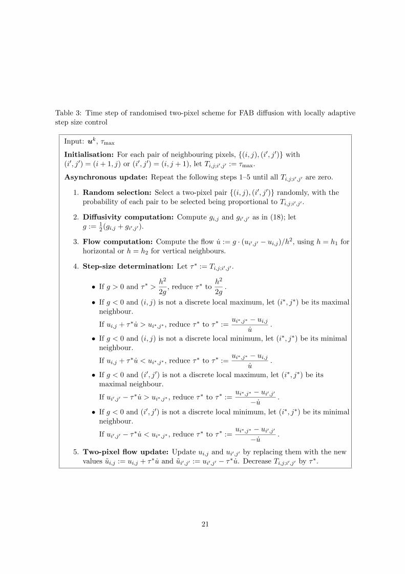
Table 3: Time step of randomised two-pixel scheme for FAB diffusion with locally adaptivestep size control

Input: uk, τmax

Initialisation: For each pair of neighbouring pixels, (i, j), (i′, j′) with(i′, j′) = (i+ 1, j) or (i′, j′) = (i, j + 1), let Ti,j;i′,j′ := τmax.

Asynchronous update: Repeat the following steps 1–5 until all Ti,j;i′,j′ are zero.

1. Random selection: Select a two-pixel pair (i, j), (i′, j′) randomly, with theprobability of each pair to be selected being proportional to Ti,j;i′,j′ .

2. Diffusivity computation: Compute gi,j and gi′,j′ as in (18); letg := 1

2(gi,j + gi′,j′).

3. Flow computation: Compute the flow u := g · (ui′,j′ − ui,j)/h2, using h = h1 forhorizontal or h = h2 for vertical neighbours.

4. Step-size determination: Let τ∗ := Ti,j;i′,j′ .

• If g > 0 and τ∗ >h2

2g, reduce τ∗ to

h2

2g.

• If g < 0 and (i, j) is not a discrete local maximum, let (i∗, j∗) be its maximalneighbour.

If ui,j + τ∗u > ui∗,j∗ , reduce τ∗ to τ∗ :=ui∗,j∗ − ui,j

u.

• If g < 0 and (i, j) is not a discrete local minimum, let (i∗, j∗) be its minimalneighbour.

If ui,j + τ∗u < ui∗,j∗ , reduce τ∗ to τ∗ :=ui∗,j∗ − ui,j

u.

• If g < 0 and (i′, j′) is not a discrete local maximum, let (i∗, j∗) be itsmaximal neighbour.

If ui′,j′ − τ∗u > ui∗,j∗ , reduce τ∗ to τ∗ :=ui∗,j∗ − ui′,j′

−u.

• If g < 0 and (i′, j′) is not a discrete local minimum, let (i∗, j∗) be its minimalneighbour.

If ui′,j′ − τ∗u < ui∗,j∗ , reduce τ∗ to τ∗ :=ui∗,j∗ − ui′,j′

−u.

5. Two-pixel flow update: Update ui,j and ui′,j′ by replacing them with the newvalues ui,j := ui,j + τ∗u and ui′,j′ := ui′,j′ − τ∗u. Decrease Ti,j;i′,j′ by τ∗.

21

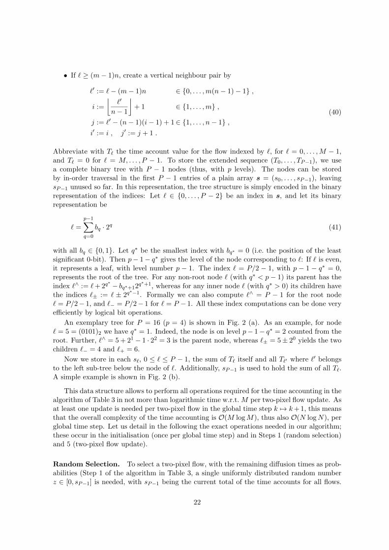
• If ` ≥ (m− 1)n, create a vertical neighbour pair by

`′ := `− (m− 1)n ∈ 0, . . . ,m(n− 1)− 1 ,

i :=

⌊`′

n− 1

⌋+ 1 ∈ 1, . . . ,m ,

j := `′ − (n− 1)(i− 1) + 1∈ 1, . . . , n− 1 ,i′ := i , j′ := j + 1 .

(40)

Abbreviate with T` the time account value for the flow indexed by `, for ` = 0, . . . ,M − 1,and T` = 0 for ` = M, . . . , P − 1. To store the extended sequence (T0, . . . , TP−1), we usea complete binary tree with P − 1 nodes (thus, with p levels). The nodes can be storedby in-order traversal in the first P − 1 entries of a plain array s = (s0, . . . , sP−1), leavingsP−1 unused so far. In this representation, the tree structure is simply encoded in the binaryrepresentation of the indices: Let ` ∈ 0, . . . , P − 2 be an index in s, and let its binaryrepresentation be

` =

p−1∑q=0

bq · 2q (41)

with all bq ∈ 0, 1. Let q∗ be the smallest index with bq∗ = 0 (i.e. the position of the leastsignificant 0-bit). Then p− 1− q∗ gives the level of the node corresponding to `: If ` is even,it represents a leaf, with level number p − 1. The index ` = P/2 − 1, with p − 1 − q∗ = 0,represents the root of the tree. For any non-root node ` (with q∗ < p− 1) its parent has theindex `∧ := `+ 2q

∗ − bq∗+12q∗+1, whereas for any inner node ` (with q∗ > 0) its children have

the indices `± := ` ± 2q∗−1. Formally we can also compute `∧ = P − 1 for the root node

` = P/2− 1, and `− = P/2− 1 for ` = P − 1. All these index computations can be done veryefficiently by logical bit operations.

An exemplary tree for P = 16 (p = 4) is shown in Fig. 2 (a). As an example, for node` = 5 = (0101)2 we have q∗ = 1. Indeed, the node is on level p− 1− q∗ = 2 counted from theroot. Further, `∧ = 5 + 21 − 1 · 22 = 3 is the parent node, whereas `± = 5± 20 yields the twochildren `− = 4 and `+ = 6.

Now we store in each s`, 0 ≤ ` ≤ P − 1, the sum of T` itself and all T`′ where `′ belongsto the left sub-tree below the node of `. Additionally, sP−1 is used to hold the sum of all T`.A simple example is shown in Fig. 2 (b).

This data structure allows to perform all operations required for the time accounting in thealgorithm of Table 3 in not more than logarithmic time w.r.t. M per two-pixel flow update. Asat least one update is needed per two-pixel flow in the global time step k 7→ k+ 1, this meansthat the overall complexity of the time accounting is O(M logM), thus also O(N logN), perglobal time step. Let us detail in the following the exact operations needed in our algorithm;these occur in the initialisation (once per global time step) and in Steps 1 (random selection)and 5 (two-pixel flow update).

Random Selection. To select a two-pixel flow, with the remaining diffusion times as prob-abilities (Step 1 of the algorithm in Table 3, a single uniformly distributed random numberz ∈ [0, sP−1] is needed, with sP−1 being the current total of the time accounts for all flows.

22

s0

s1

s2

s3

s4

s5

s6

s7

s8

s9

s10

s11

s12

s13

s14

s15(a)

0.1

0.2

0.1

0.4

0.1

0.2

0.1

0.8

0.1

0.2

0.1

0.4

0.1

0.1

0.0

1.3(b)

Figure 2: (a) Binary tree used for the time accounting of two-pixel flows in the randomisedscheme, schematic for P = 16, and its representation in an array s with additional entrys15. (b) Same binary tree with entries corresponding to M = 13 (e.g. for a 2× 5-image) andT` = 0.1 for ` = 0, . . . , 12.

By binary subdivision of the interval using the threshold values stored in the search tree, theflow index ` with

`−1∑`′=0

T`′ < z ≤∑`′=0

T`′ (42)

is determined. In detail, this is done by the following algorithm:

1. Compute a (pseudo-) random number r with uniform distribution in [0, 1].Let z = r · sP−1, and ` = P/2− 1.

2. If z ≤ s`, let β := 0, otherwise β := 1.

3. If ` is even, select the flow with index `+ β, stop.

4. If β = 0, replace ` with its left child index `−.if β = 1, decrease z by s`, then replace ` with its right child index `+.

5. Repeat from Step 2.

As an example, let the tree from Fig. 2 be given. With the pseudo-random number r = 0.45we get z = r · s15 = 0.585. Starting from ` = 7 we compare z = 0.585 ≤ s7 = 0.8, so descendto the left sub-tree, setting `− = 3 as the new `. The next comparison z = 0.585 > s3 = 0.4sends us down the right sub-tree, setting `+ = 5 as new `, and z − s3 = 0.185 as new z.Due to z = 0.185 ≤ s5 = 0.2 we replace ` with `− = 4 to descend to the left again. Now,z = 0.185 > s4 = 0.1 implies that β = 1, and ` + β = 5 is returned as index of the selectedpixel pair. Indeed, in the example

∑4`′=0 T`′ = 0.5 < 0.585 ≤

∑5`′=0 T`′ = 0.6 holds. Assuming

m = 2, n = 5, the index ` = 5 would be translated via (40) into the pixel pair (1, 1), (1, 2).

Updating of the Time Accounts. After updating the flow with index ` by the diffusiontime chunk τ∗, its time account must be updated (in Step 5 of the algorithm in Table 3).This means that all partial sums of time accounts stored in s which include T` as summandmust be decreased by τ∗. This is done as follows.

1. Decrease s` by τ∗.

23

2. If ` = P − 1, Stop.

3. Determine `∧.

If ` is the left child of `∧, i.e., (`∧)− = `, replace ` with `∧ and go to Step 1.

Otherwise replace ` with `∧ and go to Step 2.

Alternatively, one can generate a set of indices `0, . . . , `p−1 where `0 := `, and each `q+1

is obtained by flipping the bq bit of `q to 1. For each index `′ in the set, the correspondings`′ is decreased by τ∗. Note that whenever `q+1 = `q, these count as a single set element, andthe decrement is done only once.

Continuing the previous example, an update of the pixel pair belonging to ` = 5 wouldtrigger updates of the entries s5, s7 and s15.

Initialisation of the Data Structure. In the initialisation step of Table 3 that is per-formed once per global time step, the initial entries s` must be computed. In the simplestcase this is done by filling s with zeros, and performing one update with −τmax per flow.The cost of these operations is O(M logM). Further algorithmic optimisations allow to re-duce the effort to O(M). We do not pursue this optimisation here because of the marginalcontribution of the initialisation to the total computational expense, and the fact that therandom selection and two-pixel updates do not allow to reduce the overall complexity of timeaccounting below O(M logM) anyway.

6.4 Deterministic Two-Pixel Scheme with Local Step-Size Adaptation

The O(τ/h3) contribution to the approximation error that limits the conditional consistencyof the scheme from Table 3 results from the asynchronicity in the flow updates entering thevalues ui,j , ui′,j′ in the computation of each next upcoming two-pixel flow u. The order of thisapproximation error can be improved by one factor h if it is ensured that all flows contributingto each of the pixels ui,j , ui′,j′ are updated to a synchronous time level, and by another factorh if the time levels of both pixels are synchronous when the new two-pixel flow is computed.To this end, we devise another variant of an explicit two-pixel scheme with local time stepadaptation.

Pixel Updating by Total Velocities. From the randomised two-pixel scheme of Subsec-tion 6.3, we retain the principle of asynchronous updates for two-pixel flows between neigh-bouring pixels, where the maximal evolution time updates are determined such that stabilityconditions are warranted. However, whereas in Section 6.3 the isolated flows ϕi,j;i′,j′ :=g · (ui,j − ui′,j′)/h2 were used for updating pixels (i, j), (i′, j′), we use now total velocities:Each update to a pixel ui,j is made using the total velocity ui,j that incorporates the contri-butions ϕi,j;i′′,j′′ from all neighbours (i′′, j′′) of (i, j). The same goes for pixel (i′, j′).

The use of total velocities for pixel updates ensures that at each intermediate step, each ui,jis an approximation of u at location (i, j) and time kτmax + ti,j , where kτmax ≤ kτmax + ti,j ≤(k + 1)τmax, and improves the approximation error by a factor h from O(τ/h3) to O(τ/h2).Time levels ti,j for individual pixels are tracked in the algorithm.

Two-Pixel Expiry Times. The maximal evolution time Ti,j;i′,j′ up to which the pair(i, j), (i′, j′) can be updated without violating a stability condition is determined depending

24

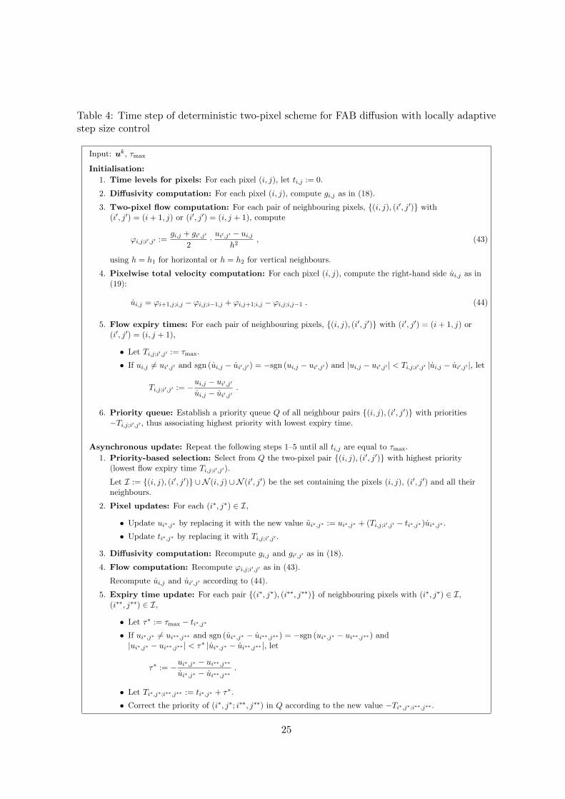
Table 4: Time step of deterministic two-pixel scheme for FAB diffusion with locally adaptivestep size control

Input: uk, τmax

Initialisation:

1. Time levels for pixels: For each pixel (i, j), let ti,j := 0.

2. Diffusivity computation: For each pixel (i, j), compute gi,j as in (18).

3. Two-pixel flow computation: For each pair of neighbouring pixels, (i, j), (i′, j′) with(i′, j′) = (i+ 1, j) or (i′, j′) = (i, j + 1), compute

ϕi,j;i′,j′ :=gi,j + gi′,j′

2·ui′,j′ − ui,j

h2, (43)

using h = h1 for horizontal or h = h2 for vertical neighbours.

4. Pixelwise total velocity computation: For each pixel (i, j), compute the right-hand side ui,j as in(19):

ui,j = ϕi+1,j;i,j − ϕi,j;i−1,j + ϕi,j+1;i,j − ϕi,j;i,j−1 . (44)

5. Flow expiry times: For each pair of neighbouring pixels, (i, j), (i′, j′) with (i′, j′) = (i+ 1, j) or(i′, j′) = (i, j + 1),

• Let Ti,j;i′,j′ := τmax.

• If ui,j 6= ui′,j′ and sgn (ui,j − ui′,j′) = −sgn (ui,j − ui′,j′) and |ui,j − ui′,j′ | < Ti,j;i′,j′ |ui,j − ui′,j′ |, let

Ti,j;i′,j′ := −ui,j − ui′,j′ui,j − ui′,j′

.

6. Priority queue: Establish a priority queue Q of all neighbour pairs (i, j), (i′, j′) with priorities−Ti,j;i′,j′ , thus associating highest priority with lowest expiry time.

Asynchronous update: Repeat the following steps 1–5 until all ti,j are equal to τmax.

1. Priority-based selection: Select from Q the two-pixel pair (i, j), (i′, j′) with highest priority(lowest flow expiry time Ti,j;i′,j′).

Let I := (i, j), (i′, j′) ∪ N (i, j) ∪N (i′, j′) be the set containing the pixels (i, j), (i′, j′) and all theirneighbours.

2. Pixel updates: For each (i∗, j∗) ∈ I,

• Update ui∗,j∗ by replacing it with the new value ui∗,j∗ := ui∗,j∗ + (Ti,j;i′,j′ − ti∗,j∗)ui∗,j∗ .• Update ti∗,j∗ by replacing it with Ti,j;i′,j′ .

3. Diffusivity computation: Recompute gi,j and gi′,j′ as in (18).

4. Flow computation: Recompute ϕi,j;i′,j′ as in (43).

Recompute ui,j and ui′,j′ according to (44).

5. Expiry time update: For each pair (i∗, j∗), (i∗∗, j∗∗) of neighbouring pixels with (i∗, j∗) ∈ I,(i∗∗, j∗∗) ∈ I,

• Let τ∗ := τmax − ti∗,j∗• If ui∗,j∗ 6= ui∗∗,j∗∗ and sgn (ui∗,j∗ − ui∗∗,j∗∗) = −sgn (ui∗,j∗ − ui∗∗,j∗∗) and|ui∗,j∗ − ui∗∗,j∗∗ | < τ∗ |ui∗,j∗ − ui∗∗,j∗∗ |, let

τ∗ := −ui∗,j∗ − ui∗∗,j∗∗

ui∗,j∗ − ui∗∗,j∗∗.

• Let Ti∗,j∗;i∗∗,j∗∗ := ti∗,j∗ + τ∗.

• Correct the priority of (i∗, j∗; i∗∗, j∗∗) in Q according to the new value −Ti∗,j∗;i∗∗,j∗∗ .

25

on the current values ui,j , ui′,j′ and velocities ui,j , ui′,j′ . We will call Ti,j;i′,j′ expiry time.In each two-pixel update step, we select the pair of neighbouring pixels with earliest expirytime.

All critical events regarding the L∞-stability of the discrete FAB diffusion process consistin pairs of neighbouring pixels reaching the same value. Therefore, each pair of neighbouringpixels (i, j), (i′, j′) is assigned an expiry time Ti,j;i′,j′ which is either the maximal diffusiontime until the next global synchronisation step, i.e. τmax − ti,j , or the time to the collision ofthe two intensities if this occurs earlier. Once a flow ϕi,j;i′,j′ is computed, it is used until itexpires, i.e. it enters all possible recomputations of ui,j and ui′,j′ as long as ti,j , ti′,j′ < Ti,j;i′,j′ .Recomputation of a neighbouring flow ϕi,j;i′′,j′′ or ϕi′,j′;i′′,j′′ with (i′′, j′′) 6= (i, j), (i′, j′) doesnot trigger a recomputation of ϕi,j;i′,j′ . However, the expiry time Ti,j;i′,j′ is adjusted in thiscase.

Updating Two-Pixel Flows and Total Velocities. After updating the flow between twoneighbouring pixels (i, j), (i′, j′) to its expiry time, it is necessary to recompute the isolatedflow ϕi,j;i′,j′ between these two pixels, and the total velocities ui,j , ui′,j′ . With regard to theabove discussion of the approximation error, we should ensure that for the computation ofϕi,j;i′,j′ all participating pixels share the same time level. This means that we cannot restrictthe pixel updates for the flow (i, j); (i′, j′) to the two pixels (i, j), (i′, j′) but must evenupdate all their neighbours (i′′, j′′) to the same time level, ti′′,j′′ = ti,j = ti′,j′ . Note that wehave selected (i, j), (i′, j′) as the two-pixel pair with earliest expiry time. Therefore, theupdates to both pixels and all their neighbours can safely be done within the expiry times ofall adjacent flows.

After synchronising in this way all participating pixels, we compute new values gi,j , gi′,j′

and a new ϕi,j;i′,j′ . The synchronisation of all pixels entering the computation of ϕi,j;i′,j′

warrants a further improvement of the approximation error by a factor h from O(τ/h2) toO(τ/h).

Adjusting Expiry Times. It is worth noticing that despite the update of all neighbouringpixels (i′′, j′′) of (i, j) and (i′, j′), the flow ϕi,j;i′,j′ is the only one that is updated. The flowsϕi,j;i′′,j′′ and ϕi′,j′;i′′,j′′ to neighbours (i′′, j′′) 6= (i, j), (i′, j′) are left unchanged, despite the factthat they depend on gi,j , gi′,j′ , too. However, their recomputation would require updates tofurther neighbour pixels, and entail total velocity updates for further pixels, and by recursionfinally lead to a synchronous time step for the entire image. By updating only ϕi,j;i′,j′ , totalvelocity updates are limited to the two pixels (i, j), (i′, j′).

We must, however, adjust the expiry times Ti,j;i′′,j′′ , Ti′,j′;i′′,j′′ for all neighbour pairs(i, j), (i′′, j′′) and (i′, j′), (i′′, j′′), because these depend on the total velocities ui,j , ui′,j′

that have changed.

Summary of the New Scheme. Plugging the aforementioned steps together, we obtainour new scheme one synchronisation step of which is summarised in Table 4. In this scheme,each pixel (i, j) is assigned a time account ti,j that starts from zero, and must reach τmax atthe end of the asynchronous update loop.

Whenever a two-pixel flow (i, j), (i′, j′) is selected for update,

26

• both pixels and all their neighbours are updated to a common time level with theirrespective total velocities; the common time level is determined by the expiry time ofthe two-pixel flow;

• the diffusivities gi,j and gi′,j′ are recomputed;

• with these new diffusivities, the flow ϕi,j;i′,j′ between the two pixels is recomputed, andthe total velocities ui,j and ui′,j′ are updated;

• the expiry times for the two-pixel flow between (i, j) and (i′, j′) as well as all two-pixelflows between (i, j), (i′, j′) and their neighbours are updated.

Comparison with Randomised Two-Pixel Scheme. As mentioned above, we have toselect two-pixel flows for update in a priority order given by their expiry times. Thereby,the selected flow always has an expiry time less or equal the expiry times of all neighbouringpairs.

The necessity to update flows in priority order implies that our new scheme is deter-ministic. The randomisation of the update order that served to avoid directional bias inSubsection 6.3 is not feasible here. However, there is also no need for such a measure here:Since each two-pixel diffusivity is recomputed if and only if it has expired, the order of updatesamong flows with equal expiry times does not change the intensities computed.

A final point to consider is that the conservation property of discretised diffusion wasensured in the randomised two-pixel scheme by always applying a two-pixel flow to bothparticipating pixels at the same time. In our new scheme, these updates may be distributedto different iterations of the asynchronous update. However, each particular value of thetwo-pixel flow ϕi,j;i′,j′ lives for a well-defined time interval [t1, t2]. It is computed when bothpixels (i, j), (i′, j′) are synchronised at time level ti,j = ti′,j′ = t1, and expires finally at a timelevel t2. All updates of ui,j and ui′,j′ until they are both synchronised at ti,j = ti′,j′ = t2 usethe same value of ϕi,j;i′,j′ , which again guarantees the conservation property.

6.4.1 Consistency of the Scheme

Adapting our argument from Section 6.3.1, we see that in the computation of ui,j , asyn-chronicity takes place only between the time levels of the approximations of flows ϕi,j;i′,j′

between (i, j) and its neighbours (i′, j′). As these flows approximate g · ux/h for horizon-tal or g · uy/h for vertical neighbours, the resulting approximation error of ui,j due to theasynchronicity is O((ux + uy)τ/h) = O(τ/h). As a result, the scheme from Table 4 has anapproximation error of O(τ + h2 + τ/h). This ensures a conditionally consistent approxima-tion to the FAB diffusion PDE if τ/h2 is bounded by a constant when τ, h → 0. However,this is always satisfied by the stability conditions of our automatic time step size adaptation.

6.4.2 Efficient Time Accounting and Flow Selection

Time accounting occurs in this algorithm in two forms: on one hand the evolution timesreached by the individual pixels have to be tracked; on the other hand two-pixel flows areequipped with expiry times. Each of the two sets of time variables can be stored in an array.

27

However, it is crucial for the algorithm that the selection of the next two-pixel flow to beupdated, namely the one with earliest expiry time, is performed efficiently. This requires anefficient implementation of the priority queue Q that stores two-pixel pairs with their expirytimes. For this purpose, a binary heap can be used, see e.g. [16, Ch. 6]. Each heap elementstores the index of the flow pair by which its expiry time can be accessed by O(1) array access.The initialisation of Q can be performed in O(M) where M is the number of two-pixel pairsas before. In the asynchronous update cycle, the highest-priority entry can be determined inO(1).

As it is necessary to adjust priorities during the operation of the algorithm, the implemen-tation must be extended into an addressable priority queue. As heap elements already storethe indices of their flow pairs, this is easily achieved by establishing an array addressed by theflow pairs, which stores for each pair a pointer to the corresponding heap element. Duringheap operations, these pointers must be kept current. This does not change the asymptoticcomplexities stated before. The heap order corrections needed to adjust the priority of anelement require not more than O(logM) operations.

Data Structure. For convenience, we shortly describe how the priority queue Q is realisedin our algorithm, adapting the binary heap construction from [16, Ch. 6]. First, the expirytimes Ti,j;i′,j′ are stored in an array T of size M , where each flow is identified by a uniqueflow-index l = li,j;i′,j′ ∈ 1, . . . ,M, and T [l] stores the expiry time of that flow. The heaparray H of size M , addressed by heap indices k running from 1 to M , stores a permutationof the flow indices 1, . . . ,M . A third array P , addressed by flow-indices, stores for each l thecorresponding heap index P [l] = k that addresses l in the heap array, such that H[P [l]] = land P [H[k]] = k for all k, l. Whenever entries of H are permuted, P must be updatedaccordingly.

For two flow indices l, l′ we define l l′ if and only if T [l] ≤ T [l′], i.e. flow l expires notlater than flow l′. The array H is in heap order (w.r.t. the expiry times T ) if and only ifH[bk/2c] H[k] for all k ∈ 2, . . . ,M. By requiring the relation between entries bk/2cand k, the array H is implicitly equipped with a binary tree structure where H[1] is the root,and each H[k] has the children H[2k] and H[2k+ 1] as long as these are inside H. Each nodeis required to be less or equal each of its children w.r.t. . As a consequence, the root H[1] isthe minimal element w.r.t. . The binary tree has the minimal possible depth, with dlog2Meas the maximal distance of a node from the root.

Priority Queue Operations. As mentioned before, the flow l with minimal expiry timeis given by H[1], and can therefore be selected in O(1) time. This is exactly what is neededin the priority-based selection step of our algorithm (asynchronous update, Step 1).

In the course of the algorithm, we need furthermore to establish the heap order (in theinitialisation Step 6), and to correct the priority of an individual flow l after a change of T [l](end of asynchronous update, Step 5).

The latter task is accomplished by two recursive procedures called sift-up and sift-down.The procedure sift-up takes a heap index k as argument. Its pre-condition is that the heaporder in H holds with the possible exception that element H[k] may violate this order bybeing placed “too low” in the tree. Then, sift-up acts by swapping H[k] up the tree untilcomplete heap order of H is restored:

28

sift-up(k) :

1. If k = 1, stop.

2. Let k′ = bk/2c.Check if H[k′] H[k]. If this is the case, stop.

3. Swap H[k] and H[k′].Update P [H[k]] = k and P [H[k′]] = k′.Call sift-up(k′).

The other procedure, sift-down, too, takes a heap index k as argument. Contrary to sift-up, it has the pre-condition that the heap order in H holds in the sub-trees below k (i.e. theroots of which are the children of k) but H[k] may violate the heap order by being placed“too high” in the tree. Then, sift-down extends the heap order to the complete tree rootedat k by swapping H[k] down the tree as far as necessary:

sift-down(k) :

1. If 2k > M , stop.

2. If 2k+ 1 ≤M and H[2k+ 1] H[2k], let k′ = 2k+ 1; otherwise, let k′ = 2k.

3. Check if H[k] H[k′]. If this is the case, stop.

4. Swap H[k] and H[k′].Update P [H[k]] = k and P [H[k′]] = k′.Call sift-down(k′).

As the recursion in both sift-up and sift-down visits each depth-plane of the binary tree atmost once, the complexity of each is O(logM). The correction of the priority of a two-pixelflow (asynchronous update, Step 5 of Table 4) is done by calling either sift-down or sift-up,depending on whether the expiry time has been increased or decreased.

The remaining task is to establish the heap order to initialise the priority queue. To thisend, H is filled by an arbitrary permutation of 1, . . . ,M (initially just (1, . . . ,M), in latertime steps just the left-over from the previous iteration). Then one calls sift-down(k) fork = bM/2c, . . . , 1 in descending order. As the heap order condition is trivially satisfied ineach single-node subtree, the heap order in H holds right of k before the call to sift-down(k),and holds from k on to the right after this call. Analysis of the run time, see [16, Ch. 6],shows that the complexity of establishing the heap order on H is O(M).

Final Remark. For our algorithm, the binary heap structure as described offers a fair bal-ance of simplicity and efficiency. Further (slight) performance gains can possibly be achievedby using more sophisticated implementations of addressable priority queues; see [16, Ch. 6].

7 Experiments

For our experiments below, we use test images with quadratic pixels, where we assume unitgrid size h1 = h2 = 1. The greyscale range lies in the interval [0, 255]. We have implementedour methods in ANSI C and compiled the code with a GNU gcc compiler (version 5.4.0). The

29

parallel algorithm from Section 6.2 was implemented in CUDA C, and compiled using theNvidia R© CUDA compilation tools (version 8.0.44). Compiler optimisation was set to -O2 inall cases, CUDA architecture was set to 6.1. No advanced code optimisations took place.

For CPU algorithms, we report run times on a single core of a workstation with an Intel R©

CoreTM i7-6800K CPU running at 3.40 GHz. CUDA computations were performed on thesame machine, using a Zotac GeForce GTX 1080 graphics card with 8 GB RAM and 2560compute units.

7.1 Standard vs. Nonstandard Discretisation

In our first experiment we compare two implementation of our explicit scheme (19): one withthe standard discretisation (17), the other one with the nonstandard discretisation (18). Weuse the diffusivity function (5). Fig. 3 shows the results for a standard test image that isprocessed with FAB diffusion with λ = 4, κ = 2.5, and stopping time t = 10. We observethat an explicit scheme with standard discretisation is unstable, even for very small time stepsizes (Fig. 3(b)). Thus, it is not considered any further.

Equipping the explicit scheme with the nonstandard discretisation allows to come upwith a stable result, provided that the time step size limit (20) is obeyed (Fig. 3(c)). Forthe diffusivity (5) with λ = 4 and κ = 2.5, the constant ω in (20) is given by ω = 0.009568.Together with the grid sizes h1 = h2 = 1 this yields a time step size restriction of τ ≤1.14 ·10−5. Choosing τ := 1 ·10−5 requires as many as 1 million iterations to reach a stoppingtime of t = 10. The corresponding CPU time was approx. 50 minutes. Since this is too slowfor most applications, let us have a look at our various acceleration strategies.

7.2 Faster Algorithms

The remaining images (d)–(f) in Fig. 3 show the results for three accelerations of the ex-plicit scheme with nonstandard discretisation: global step size adaptation (Subsection 6.1),the randomised two-pixel scheme (Subsection 6.3), and its deterministic variant (Subsection

Table 5: Run times (in seconds) for the computation of the results in Fig. 3 by CPU and CUDAimplementations. CUDA-d refers to a version with double precision, whereas in CUDA-df thediffusivities g are computed in single precision. For CUDA, upright numbers show the grossrun time of the program, whereas numbers in italics show the net computation time withoutsystem overheads.

Algorithm CPU CUDA-d CUDA-df

explicit/standard discr. 2784explicit/nonstandard discr. 3004 42.5 26.3

36.3 19.9global time step adaptation 24.1 0.84 0.79

0.30 0.23randomised two-pixel 8.6 — —deterministic two-pixel 3.5 — —

30

6.4). We observe that all approaches are visually of the same quality than its nonacceleratedcounterpart. However, as evident from Table 5, they offer substantial speed-ups:

• The scheme with global time step adaptation and a maximal time step size of 0.24requires only 4710 iterations to reach the stopping time of t = 10. Thus, its averagetime step size is about 210 times larger than the baseline scheme. This shows that ourtime step size restriction (20) based on a priori estimates is indeed very pessimistic.

With 24 seconds, the computation time has reduced by a factor of about 120. Comparingthis to the factor 210 for the time step size, the additional expense of the time stepadaptation is visible.

• For the randomised two-pixel variant of the explicit scheme with nonstandard discreti-sation we use a sync step size of τmax = 0.1. Thus, only 100 sync steps are necessaryto reach a stopping time of t = 10. This requires a CPU time of 8.6 seconds, i.e. aspeed-up of 2.8 compared to the scheme with global time step adaptation, or about 350compared to the explicit scheme with constant time step size.

The fact that the average time step size of 0.0991 is very close to the sync step sizeof = 0.1 demonstrates that time step size reductions for stability reasons are very rareevents.

• The deterministic two-pixel scheme with a sync step size of τmax = 0.1 is even fasterthan its probabilistic counterpart: Its run time comes down to 3.5 seconds, amountingto a speed-up of 2.4 over the scheme from Section 6.3, of 6.8 over the scheme with globaltime step adaptation, and of 850 over the scheme with fixed time steps.

CUDA implementations were done for the explicit scheme with nonstandard discretisation,and for the scheme with global time step adaptation. Asynchronous schemes with local timestep adaptation do not lend themselves to a straightforward parallelisation. The explicitscheme with standard discretisation could easily be parallelised but is not worth the effortdue to its instability. A word of care should be said about numerical precision. Unlike inmany diffusion-based algorithms in image processing,, where single-precision float numbersare accurate enough, double precision is necessary in all of our algorithms due to the extremelysmall time steps that occur. Whereas on modern CPUs there is no noticeable difference in runtimes between single and double precision, precision still matters for performance on graphicscards. Our comparison therefore includes two variants of the CUDA implementation: one inwhich all numerical computations are performed in double precision (CUDA-d in Table 5),and one in which double precision is used for u, u and time steps, whereas the diffusivitiesg are computed only in single precision, as a closer analysis reveals that the higher precisionis not necessary for g (CUDA-df in Table 5). Numerical deviations between the CPU andboth CUDA implementations for each algorithms were negligible (note that differences in theorder of machine precision occur regularly between CPU and CUDA).

For the CUDA implementations, we report in Table 5 the gross run times of the programrun and (in italics) the net computation times. The latter exclude some system overheadsthat occur due to the management of the graphics card, and contribute considerably to theoverall program run time. For CPU computations, such system overheads are not observed.

As expected, the CUDA implementations allow further accelerations of the two first algo-rithms. With 42 (36 ) seconds for the explicit scheme with fixed time steps, and 0.84 (0.30)

31

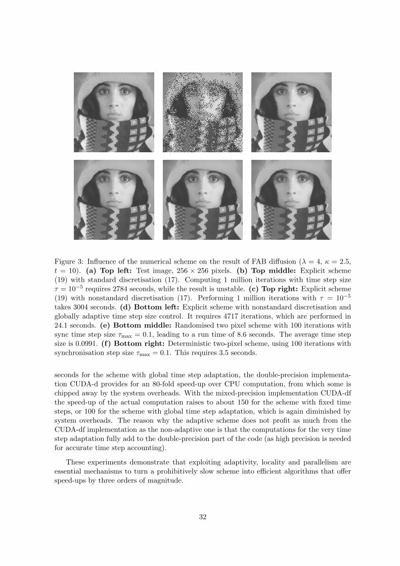
Figure 3: Influence of the numerical scheme on the result of FAB diffusion (λ = 4, κ = 2.5,t = 10). (a) Top left: Test image, 256 × 256 pixels. (b) Top middle: Explicit scheme(19) with standard discretisation (17). Computing 1 million iterations with time step sizeτ = 10−5 requires 2784 seconds, while the result is unstable. (c) Top right: Explicit scheme(19) with nonstandard discretisation (17). Performing 1 million iterations with τ = 10−5

takes 3004 seconds. (d) Bottom left: Explicit scheme with nonstandard discretisation andglobally adaptive time step size control. It requires 4717 iterations, which are performed in24.1 seconds. (e) Bottom middle: Randomised two pixel scheme with 100 iterations withsync time step size τmax = 0.1, leading to a run time of 8.6 seconds. The average time stepsize is 0.0991. (f) Bottom right: Deterministic two-pixel scheme, using 100 iterations withsynchronisation step size τmax = 0.1. This requires 3.5 seconds.

seconds for the scheme with global time step adaptation, the double-precision implementa-tion CUDA-d provides for an 80-fold speed-up over CPU computation, from which some ischipped away by the system overheads. With the mixed-precision implementation CUDA-dfthe speed-up of the actual computation raises to about 150 for the scheme with fixed timesteps, or 100 for the scheme with global time step adaptation, which is again diminished bysystem overheads. The reason why the adaptive scheme does not profit as much from theCUDA-df implementation as the non-adaptive one is that the computations for the very timestep adaptation fully add to the double-precision part of the code (as high precision is neededfor accurate time step accounting).

These experiments demonstrate that exploiting adaptivity, locality and parallelism areessential mechanisms to turn a prohibitively slow scheme into efficient algorithms that offerspeed-ups by three orders of magnitude.

32

t = 0 t = 6 t = 80

t = 200 t = 800 t = 3000

Figure 4: Temporal evolution of FAB diffusion (λ = 2, κ = 2.5), applied to a noisy test imagewith 256 × 256 pixels. The computations have been done with the deterministic two-pixelscheme with sync step size τmax = 0.1.

7.3 Scale-Space Behaviour

Since our accelerated algorithms are highly efficient, they can also be used for long termcomputations, arising e.g. in scale-space analysis [11, 39]. Fig. 4 depicts the temporal evolutionof a noisy test image when the scale-space is governed by FAB diffusion with diffusivity (5),and the deterministic two-pixel scheme is employed. We observe the high robustness of theFAB scale-space in spite of the fact that its diffusities may become negative. Moreover, theexperiment confirms convergence to a flat steady state for t→∞. This is in full accordancewith our theoretical results.

7.4 Different Types of FAB Diffusivities

The crucial assumption for our theory is that g(0) > 0, which ensures that extrema undergoforward diffusion.

Thus, we do not only not require the diffusivity to take positive values for large gradients.Our framework can handle even diffusivities tending to negative limits for infinite gradients.An example is shown in Figure 5(g). For gradients going to infinity, the corresponding pe-naliser functions always decrease unboundedly; see the example in Figure 5(h).

To summarise, we focus on three main classes of diffusivities:

33

-1

-0.5

0

0.5

1

0 2 4 6 8 10 12 14

-6

-4

-2

0

2

4

6

0 2 4 6 8 10 12 14

(a) Diffusivity, Type I (b) Penaliser corresponding to (a)

-1

-0.5

0

0.5

1

0 2 4 6 8 10 12 14

-4

-2

0

2

4

0 2 4 6 8 10 12 14

(c) Diffusivity, Type II (d) Penaliser corresponding to (c)

-1

-0.5

0

0.5

1

0 2 4 6 8 10 12 14

-30

-20

-10

0

10

20

30

0 2 4 6 8 10 12 14

(e) Diffusivity, Type II (f) Penaliser corresponding to (e)

-1

-0.5

0

0.5

1

0 2 4 6 8 10 12 14

-20

-15

-10

-5

0

5

10

15

20

0 2 4 6 8 10 12 14

(g) Diffusivity, Type III (h) Penaliser corresponding to (g)

Figure 5: Forward-and-backward diffusivity functions g(s2) of Type I, Type II (two cases)and Type III, and corresponding penaliser functions Ψ(s2). The horizontal axis shows s, thevertical axis function values.

34

Type I. Diffusivities similar to that from [9] that take positive values for large gradientmagnitudes and tend to zero in the limit of infinite gradient magnitudes; see Figure 5(a).

Diffusivities of this kind can be associated to triple-well potentials, as shown in Fig-ure 5(b). Some of these potentials are bounded from below by convex functions, whichadmits the application of some theoretical results in the space-continuous case.

Type II. Diffusivities similar to those from [26] that take negative values for large gradientmagnitudes and tend to zero in the limit of infinite gradient magnitudes; see Figure 5(c)and (e).

The penaliser functions

Ψ(s2) :=

s2∫0

g(t) dt (45)

corresponding to these diffusivities may have positive or negative horizontal asymptotes,as shown in Figure 5(d) and (f), or even decrease unboundedly in other cases.

Type III. Diffusivities that tend to a negative limit for gradient magnitudes going to infinity;see Figure 5(g).

For gradient magnitudes going to infinity, the corresponding penaliser functions alwaysdecrease unboundedly, see the example in Figure 5(h).

Specific representatives for these three types of diffusivities are presented in Table 6. We usethem for our experiments in Fig. 6. We observe that our deterministic two-pixel scheme canindeed handle all three scenarios. As expected, the Type I diffusivity reveals the strongestsmoothing behaviour. The Type III diffusivity leads to the most extreme enhancement: Itspronounced backward diffusion along the edge contour produces fairly jagged edges.

8 Summary and Conclusions

Backward diffusion suffers from an extremely bad reputation of being a highly ill-posed pro-cess. We have seen in our paper that it can be turned into a highly stable evolution, providedthat some essential requirements are met:

First of all, it must be stabilised at extrema in order to avoid under- and overshoots. TheFAB diffusion paradigm does take care of this. Our discrete analysis is based on a smoothFAB diffusivity that attains a positive diffusivity in zero which is larger than the moduliof all negative diffusivities. Under these mild model assumptions we were able to establishwell-posedness, a maximum–minimum principle, and convergence to a flat steady state forspace-discrete FAB diffusions with a nonstandard discretisation of the gradient magnitude.These properties carry over to the fully discrete case with an explicit scheme, if one adheresto a very restrictive time step size limit.

In order to make this concept practically viable, we came up with a number of novelschemes that exploit adaptivity or parallelism. In the simplest case, this adaptivity wasapplied globally by varying the time step size during the evolution. Allowing even space-variant time step sizes by splitting the diffusion process into two-pixel interactions is the

35

most consequent and the most powerful implementation of the concept of adaptivity. To ourknowledge this is the first time in PDE-based image analysis where the idea of space-varianttime step sizes is used. We showed that this allows to accelerate FAB diffusion by up to threeorders of magnitude.

We hope that our results may help to improve the reputation of backward parabolicprocesses, since they can offer some very attractive image enhancement properties that havehardly been explored so far, mainly because of the lack of stable numerical schemes. In ourongoing work we are looking into other PDE-based image enhancement methods that sufferfrom ill-posed continuous formulations.

Acknowledgements

J.W. and G.G. would like to thank the Isaac Newton Institute for Mathematical Sciences forsupport and hospitality during the programme Variational Methods and Effective Algorithmsfor Imaging and Vision, when final work on this paper was undertaken. This work was sup-ported by EPSRC Grant Number EP/K032208/1 and by a Rothschild Distinguished VisitingFellowship for J.W.

References

[1] Aubert, G., Kornprobst, P.: Mathematical Problems in Image Processing: Partial Dif-ferential Equations and the Calculus of Variations, Applied Mathematical Sciences, vol.147, second edn. Springer, New York (2006)

[2] Babaud, J., Witkin, A.P., Baudin, M., Duda, R.O.: Uniqueness of the Gaussian kernelfor scale space filtering. IEEE Transactions on Pattern Analysis and Machine Intelligence8, 26–33 (1986)

Table 6: Specific representatives for our three types of FAB diffusivities.

DiffusivityType

Explicit Formula Parameters

Type I g(s2) =cos(π y(s))

1 + (y(s))2, λ1 > 0,

y(s) =5

2

((λ22 − 6λ21) s− (λ2 − 6λ1) s

2

4λ1λ2(λ2 − λ1) + (λ22 − 6λ21) s− (λ2 − 6λ1) s2

)λ2 >

√6λ1

Type II g(s2) = 2 exp

(−κ

2 ln 2

κ2 − 1· s

2

λ2

)− exp

(− ln 2

κ2 − 1· s

2

λ2

)λ > 0, κ > 1

Type III g(s2) =3

2exp

(− ln 3

λ2s2)− 1

2λ > 0

36

Type I (λ1=4, λ2=10) Type II (λ=4, κ=2.5) Type III (λ=4)

Zoom into Type I Zoom into Type II Zoom into Type III

Figure 6: Comparison of the influence of the diffusivity functions. We use the diffusivities fromTable 6. All computations are performed with the deterministic two-pixel scheme applied tothe test image from Fig. 3(a) with sync step size τmax = 0.1 and stopping time t = 10.

[3] Breuß, M., Welk, M.: Staircasing in semidiscrete stabilised inverse diffusion algorithms.Journal of Computational and Applied Mathematics 206(1), 520–533 (2007)

[4] Burgeth, B., Weickert, J., Tari, S.: Minimally stochastic schemes for singular diffusionequations. In: X.C. Tai, K.A. Lie, T.F. Chan, S. Osher (eds.) Image Processing Basedon Partial Differential Equations, pp. 325–339. Springer, Berlin (2007)

[5] Carasso, A.S.: Stable explicit time marching in well-posed or ill-posed nonlinear parabolicequations. Inverse Problems in Science and Engineering 24(8), 1364–1384 (2016)

[6] Carasso, A.S.: Stabilized Richardson leapfrog scheme in explicit stepwise computationof forward or backward nonlinear parabolic equations. Inverse Problems in Science andEngineering 25(12), 1719–1742 (2017)

[7] Elmoataz, A., Lezoray, O., Ta, V.T., Bougleux, S.: Partial difference equations on graphsfor local and nonlocal image processing. In: O. Lezoray, L. Grady (eds.) Image Processingand Analysis with Graphs: Theory and Practice, chap. 7, pp. 174–206. CRC Press, BocaRaton (2012)

[8] Gabor, D.: Information theory in electron microscopy. Laboratory Investigation 14,801–807 (1965)

37

[9] Gilboa, G., Sochen, N., Zeevi, Y.Y.: Image sharpening by flows based on triple wellpotentials. Journal of Mathematical Imaging and Vision 20, 121–131 (2004)

[10] Gilboa, G., Sochen, N.A., Zeevi, Y.Y.: Forward-and-backward diffusion processes foradaptive image enhancement and denoising. IEEE Transactions on Image Processing11(7), 689–703 (2002)

[11] Iijima, T.: Basic theory on normalization of pattern (in case of typical one-dimensionalpattern). Bulletin of the Electrotechnical Laboratory 26, 368–388 (1962). In Japanese

[12] Kovasznay, L.S.G., Joseph, H.M.: Image processing. Proceedings of the IRE 43(5),560–570 (1955)

[13] Kramer, H.P., Bruckner, J.B.: Iterations of a non-linear transformation for enhancementof digital images. Pattern Recognition 7, 53–58 (1975)

[14] Lindeberg, T.: Scale-Space Theory in Computer Vision. Kluwer, Boston (1994)

[15] Lindenbaum, M., Fischer, M., Bruckstein, A.: On Gabor’s contribution to image en-hancement. Pattern Recognition 27, 1–8 (1994)

[16] Mehlhorn, K., Sanders, P.: Algorithms and Data Structures – The Basic Toolbox.Springer, Berlin (2008)

[17] Mickens, R.E.: Nonstandard Finite Difference Models of Differential Equations. WorldScientific, Singapore (1994)

[18] Mrazek, P., Weickert, J., Steidl, G.: Diffusion-inspired shrinkage functions and stabilityresults for wavelet denoising. International Journal of Computer Vision 64(2/3), 171–186(2005)

[19] Nikolova, M.: Local strong homogeneity of a regularized estimator. SIAM Journal onApplied Mathematics 61(2), 633–658 (2000)

[20] Nikolova, M.: Minimizers of cost-functions involving nonsmooth data fidelity terms.application to the processing of outliers. SIAM Journal on Numerical Analysis 40(3),965–994 (2002)

[21] Osher, S., Rudin, L.: Shocks and other nonlinear filtering applied to image processing.In: A.G. Tescher (ed.) Applications of Digital Image Processing XIV, Proceedings ofSPIE, vol. 1567, pp. 414–431. SPIE Press, Bellingham (1991)

[22] Osher, S., Rudin, L.I.: Feature-oriented image enhancement using shock filters. SIAMJournal on Numerical Analysis 27, 919–940 (1990)

[23] Perko, L.: Differential Equations and Dynamical Systems, third edition edn. Springer,New York (2001)

[24] Perona, P., Malik, J.: Scale space and edge detection using anisotropic diffusion. IEEETransactions on Pattern Analysis and Machine Intelligence 12, 629–639 (1990)

38

[25] Pollak, I., Willsky, A.S., Krim, H.: Image segmentation and edge enhancement withstabilized inverse diffusion equations. IEEE Transactions on Image Processing 9(2),256–266 (2000)

[26] Smolka, B.: Combined forward and backward anisotropic diffusion filtering of color im-ages. In: L. Van Gool (ed.) Pattern Recognition, Lecture Notes in Computer Science,vol. 2449, pp. 314–320. Springer, Berlin (2002)

[27] Smolka, B., Plataniotis, K.N.: On the coupled forward and backward anistropic diffusionscheme for color image enhancement. In: M.S. Lew, N. Sebe, J.P. Eakins (eds.) Imageand Video Retrieval, Lecture Notes in Computer Science, vol. 2383, pp. 70–80. Springer,Berlin (2002)

[28] Steidl, G., Weickert, J., Brox, T., Mrazek, P., Welk, M.: On the equivalence of softwavelet shrinkage, total variation diffusion, total variation regularization, and SIDEs.SIAM Journal on Numerical Analysis 42(2), 686–713 (2004)

[29] Tikhonov, A.N., Arsenin, V.Y.: Solutions of Ill–Posed Problems. Wiley, Washington,DC (1977)

[30] Wang, Y., Niu, R., Shen, H., Yu, X.: Forward-and-backward diffusion for hyperspectralremote sensing image smoothing and enhancement. In: D. Li, J. Gong, H. Wu (eds.) In-ternational Conference on Earth Observation Data Processing and Analysis (ICEODPA),Proceedings of SPIE, vol. 7285. SPIE Press, Bellingham (2008)

[31] Wang, Y., Niu, R., Zhang, L., Wu, K., Sahli, H.: A scale-based forward-and-backwarddiffusion process for adaptive image enhancement and denoising. EURASIP Journal onAdvances in Signal Processing 2011(22) (2011)

[32] Wang, Y., Zhang, L., Li, P.: Local variance-controlled forward-and-backward diffusionfor image enhancement and noise reduction. IEEE Transactions on Image Processing16(7), 1854–1864 (2007)

[33] Weickert, J.: Anisotropic Diffusion in Image Processing. Teubner, Stuttgart (1998)

[34] Weickert, J., Benhamouda, B.: A semidiscrete nonlinear scale-space theory and its rela-tion to the Perona–Malik paradox. In: F. Solina, W.G. Kropatsch, R. Klette, R. Bajcsy(eds.) Advances in Computer Vision, pp. 1–10. Springer, Wien (1997)

[35] Welk, M., Gilboa, G., Weickert, J.: Theoretical foundations for discrete forward-and-backward diffusion filtering. In: X.C. Tai, K. Mørken, M. Lysaker, K.A. Lie (eds.) ScaleSpace and Variational Methods in Computer Vision, Lecture Notes in Computer Science,vol. 5567, pp. 527–538. Springer, Berlin (2009)

[36] Welk, M., Steidl, G., Weickert, J.: Locally analytic schemes: A link between diffusionfiltering and wavelet shrinkage. Applied and Computational Harmonic Analysis 24, 195–224 (2008)

[37] Welk, M., Weickert, J.: An efficient and stable two-pixel scheme for 2D forward-and-backward diffusion. In: F. Lauze, Y. Dong, A.B. Dahl (eds.) Scale Space and VariationalMethods in Computer Vision, Lecture Notes in Computer Science, vol. 10302, pp. 94–106.Springer, Cham (2017)

39

[38] Welk, M., Weickert, J., Galic, I.: Theoretical foundations for spatially discrete 1-D shockfiltering. Image and Vision Computing 25(4), 455–463 (2007)

[39] Witkin, A.P.: Scale-space filtering. In: Proc. Eighth International Joint Conference onArtificial Intelligence, vol. 2, pp. 945–951. Karlsruhe, West Germany (1983)

[40] Zakeri, A., Jannati, Q., Amiri, A.: A numerical scheme for solving nonlinear backwardparabolic problems. Bulletin of the Iranian Mathematical Society 41(6), 1453–1464(2015)

40