a d3 plug-in for automatic label placement using simulated...
TRANSCRIPT

A D3 plug-in for automatic label placement using simulatedannealing
Evan Wang
Abstract—Although labeling graphical features can help viewers quickly grasp complex nuances of the data, it is a very time-consuming process. For the majority of point-feature label placement problems, the rules are relatively straightforward. Therefore,this is a problem very much suited for automated labeling algorithms. Automatic label placement is widely used by map generators,but surprisingly, there is little evidence that individuals use it. One reason might be that for many advanced plotting tools favoredby scientists and engineers, there is often no sophisticated built-in labeling function. A possible solution is to create a plug-in (alsocalled extension or add-on) for an existing program that performs label placement. Such plug-ins do exist for some plotting programs,with varying sophistication and ease of use. In this work, I plan to write build an automatic labeling plug-in for the popular JavaScriptvisualization library D3 that implements simulated annealing and easily incorporates into existing D3 code, with syntax mirroring otherD3 layouts.
Index Terms—automatic label placement, simulated annealing, D3, plug-in
1 INTRODUCTION
Labeling features or data points, more commonly known as point-feature label placement, is an integral part of a visualization becauseit helps viewers quickly see what the data represents and points outnuances that could otherwise be overlooked. However, manually la-beling features is a very time-consuming task. According to Cook andJones, cartographers place approximately 20-30 labels per hour [1].
Given the time required to manually place labels, automatic labelplacement is used widely by map generators such as LineDrive [2].However, there is little published or empirical evidence that indicatesindividuals frequently use automatic labeling. This presents a conun-drum. Why would so many individuals manually label graphs andcharts even though doing so requires a substantial time commitment?Not only that, an optimization problem such as this is perfectly suitedfor one of many standard search/optimization algorithms available.One reason is that for advanced plotting tools (R, D3, Matlab, Math-ematica, and Matplotlib) favored by scientists and engineers, there isoften no sophisticated built-in automatic label placement function. Inorder to label a scatter plot, one often has to resort to tweaking labelsmanually. A possible solution to the problem is to create a plug-in(sometimes called extension or add-on) for an existing program thatperforms the label placement. Plug-ins do exist for some of the afore-mentioned plotting tools.
In particular for D3, an increasingly popular Javascript visualiza-tion library, there are presently label placement implementations avail-able that make use of the D3 force layout [16, 17]. However, the forcelayout (based on force-directed algorithms) is an algorithm for draw-ing graphs, specifically undirected graphs [3]. And although it canbe effectively adapted for labeling, it is not built for such a task andtherefore many of the nuances of good labeling practices cannot beimplemented. For my project I have implemented a D3 plug-in forautomatic label placement using simulated annealing that incorporatesgood label placement practices and is easy-to-use.
2 RELATED WORK
2.1 Label placement rules
The layout of a labeling problem is shown in Fig. 1. Each label cor-responds to an anchor point. A leader line may be used to help withthe correspondence between the label and anchor point [14]. Noneof the elements may cross the graph boundary. The general rules
• Author email: [email protected]
North BeachRussian Hill
Label
Leader line
Anchor pointGraph boundary
Fig. 1. Anatomy of a label problem. Each label corresponds to ananchor point. A leader line may be used to help with the correspondencebetween the label and anchor point. None of the elements may crossthe graph boundary.
for label placement have been carefully studied by many, most no-tably described by Imhof [4, 5] and more quantitatively formulated byYeoli [6]. The basic rules are:
• Spatial overlap: Labels should not overlap with each other orother point features.
• Unambiguity: Labels should be clearly and unambiguously iden-tified with its corresponding graphical feature(s).
• Legibility: Labels should be easily readable.
Comparisons of good and bad labeling practices are showin inFig. 2. Fig. 2 (a) is an example of a bad label configuration because itdoes not follow Imhof and Yeolis rules. There are several label-labeloverlaps, label-anchor overlaps, and in general a sense of randomnessin how the labels are placed. This results in ambiguity in label-pointcorrespondence and for the viewers, a longer time or even inabilityto process the data. In contrast, Fig. 2 (b) shows a much better labelconfiguration because there are no overlaps of any kind and there ex-ists a much greater readability due to the ordered nature of the labelplacements.
In addition to these rules, Imhof described a set of more specificstylistic rules pertaining to specific label positions [4]:
• Label position on the right is preferred over left.
• Label position on top is preferred over below.
• Label position closer to the corresponding point feature is pre-ferred.
A visual representation of Imhof’s stylistic rules are shown in Fig. 3.

(a)Golden Gate Park
Mission
Nob Hill
North BeachPacific Heights
Russian Hill
Western Addition
Noe Valley
Union SquareTenderloin
Golden Gate ParkMission
Nob Hill
North BeachPacific Heights Russian Hill
Western Addition
Noe Valley
Union Square Tenderloin
(b)
Fig. 2. Good and bad label placements. (a) Bad label placement :Some labels overlap with each other and/or with anchor points. In ad-dition, there are no conventions for preferred placement positions. Thiscreates ambiguity in terms of which label corresponds to which datapoint. (b) Good label placement : There are no overlaps, labels tend tobe situated in a corner of the data point, and consequently, no ambiguityfor label-data correspondence.
2.2 Search spaceSo far, our description of the problem has been qualitative (i.e. de-
scription based rules such as avoid overlaps, place labels in more pre-ferred positions). For an optimization problem such as this, we haveto first define the search space [7]. In a labeling problem, the searchspace consists of the collection of label positions. Each configurationof label positions, or state (ν), can be written as
ν = {r1,r2,r3, . . .rN}, (1)
where r = (rx,ry) is used as a shorthand to denote the position of eachlabel. Additionally, each individual component of every label positionr must satisfy the constraints of the graph boundaries,
rx > Lminx
rx < Lmaxx
ry > Lminy
ry < Lmaxy .
(2)
All label configurations that satisfy the boundary conditions are per-missible. The search space contains 2N degrees of freedom, whereN is the total number of labels. It is important to note that we haveallowed neither the fontsize of the labels nor the orientation (tilt) tobe a free parameter. Adding these elements as free parameters wouldincrease the dimensionality of the problem (an additional N degrees offreedom for each added parameter), but is otherwise entirely possibleand straightforward. However, size and orientation are mostly used incartographic applications were the various geographical features ne-cessitates their usage and utility. For label point features in graphs,features such as size and orientation are usually fixed and is the reasonfor their exclusion.
2.3 Energy functionOf course, not all points in the search space are equally preferable.
Label configurations that result in less overlap and in general adhereto label placement rules are more preferred. In Fig. 2, both (a) and (b)
Nob HillNob Hill
Nob Hill Nob Hill Nob Hill
Nob HillNob Hill Nob Hill
Fig. 3. Preferred label positions. The relative preference of the posi-tions (according to Imhof [4]) are indicated according to the color satu-ration of the label. Darker labels represent more desirable positions.
are permissible states or configurations in the search space. However,Fig. 2 (a) is the more preferred label configuration because there areless overlaps and greater readability. In order to distinguish betweenthe quality of different configurations in our search space, we needconstruct a function which takes as input a label configuration andoutputs a score indicating the quality of the placements. In a labelingproblem, the inputs are themselves functions of various parameterssuch as the amount of overlaps, distances between labels and theircorresponding anchor points, and various stylistic preferences. Thisfunction, often an energy (also called cost or objective) function, iswhat we need to optimize. Based on Imhof and Yeoli’s rules [4, 5, 6],our energy function for each individual label i depends on
Ei = f (All ,Al p,Ll p,θ), (3)
where All is the area of label-label overlaps, Al p is the area of label-point overlaps, Ll p is the distance between the label and the point, andθ is the orientation of the label relative to the point. The form of ourenergy function for label i for a system with N total labels is then
Ei =N
∑j 6=i
AllWll +N
∑j 6=i
Al pWl p +Ll pWl p +θWθ , (4)
where the W terms are weight constants signifying the relative im-portance of each rule. For each label i, we sum over all other labelsand points in order to compute the total area overlap. The greater theoverlap, the higher the resulting energy. To obtain the total energy, wesimply sum over each label, or index i
Etot =N
∑i
Ei. (5)
These are only an example of an energy function for a labeling prob-lem. Different terms can be inserted or removed based on individualpreferences.
2.4 Overview of algorithmsThe labeling problem is essentially an optimization problem on
a complex and high-dimensional energy landscape. Therefore, manypossible classes of algorithms can be applied. A shortlist of the morewell-known algorithms include random placement, exhaustive searchalgorithms, greedy algorithms, local search algorithms, stochasticsearch algorithms, genetic algorithms, and mathematical program-ming [7]. In general, these algorithms may be categorized into lo-cal search methods and global optimization methods. For the sake ofbrevity, I will give a more detailed overview for the more widely usedalgorithms.
2.4.1 Greedy algorithmIn general, a greedy algorithm makes a locally optimal choice at
every step without backtracking. As applied to label placement, thealgorithm is the following. With respect to labeling, this means thatlabels are placed serially, and each label is placed to minimize thecurrent energy, given the positions of the other labels. Algorithmically,
it is implemented as follows.while all points are not labeled do
select an unlabeled point;place label according to preset rules;if no free position then
leave out the label;orlabel point even with overlap;orask for feedback from human;
endend
Algorithm 1: Greedy algorithmGreedy algorithms are best suited for problem in which “thinking
ahead has little benefit. Physically, since we are freezing the con-figuration of all other labels, the energy landscape is always two-dimensional. With each label, we are finding the global minima of thattwo-dimensional and changing landscape. We never consider the en-tire 2N-dimensional landscape. This is the so-called myopic behaviorassociated with greedy algorithms [15]. However, the labeling prob-lem is best solved by finding a minimum on the full energy landscape,and not simply minima on two-dimensional slices of the landscape.Thus while generally very fast, the greedy algorithm frequently gener-ates label configurations that could be vastly improved [7].
2.4.2 Gradient descentAn gradient descent implementation of automatic label placement
is generally considered better than using a greedy algorithm becausewe now can fine tune a particular configuration by local label move-ments. The algorithm is as follows [8].
while convergence not reached dorandomly make several perturbations to the configuration;calculate decrease in cost function ∆E;accept the perturbation with the most negative ∆E;
endAlgorithm 2: Gradient descent
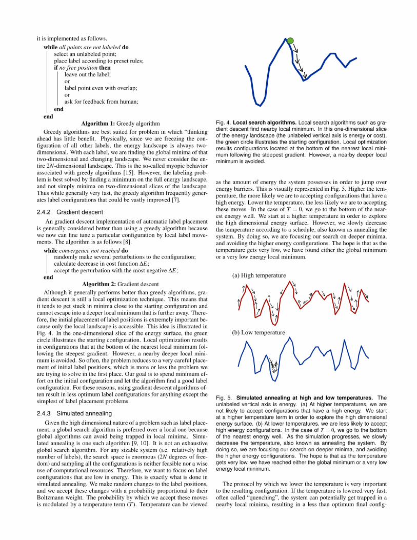
Although it generally performs better than greedy algorithms, gra-dient descent is still a local optimization technique. This means thatit tends to get stuck in minima close to the starting configuration andcannot escape into a deeper local minimum that is further away. There-fore, the initial placement of label positions is extremely important be-cause only the local landscape is accessible. This idea is illustrated inFig. 4. In the one-dimensional slice of the energy surface, the greencircle illustrates the starting configuration. Local optimization resultsin configurations that at the bottom of the nearest local minimum fol-lowing the steepest gradient. However, a nearby deeper local mini-mum is avoided. So often, the problem reduces to a very careful place-ment of initial label positions, which is more or less the problem weare trying to solve in the first place. Our goal is to spend minimum ef-fort on the initial configuration and let the algorithm find a good labelconfiguration. For these reasons, using gradient descent algorithms of-ten result in less optimum label configurations for anything except thesimplest of label placement problems.
2.4.3 Simulated annealingGiven the high dimensional nature of a problem such as label place-
ment, a global search algorithm is preferred over a local one becauseglobal algorithms can avoid being trapped in local minima. Simu-lated annealing is one such algorithm [9, 10]. It is not an exhaustiveglobal search algorithm. For any sizable system (i.e. relatively highnumber of labels), the search space is enormous (2N degrees of free-dom) and sampling all the configurations is neither feasible nor a wiseuse of computational resources. Therefore, we want to focus on labelconfigurations that are low in energy. This is exactly what is done insimulated annealing. We make random changes to the label positions,and we accept these changes with a probability proportional to theirBoltzmann weight. The probability by which we accept these movesis modulated by a temperature term (T ). Temperature can be viewed
Fig. 4. Local search algorithms. Local search algorithms such as gra-dient descent find nearby local minimum. In this one-dimensional sliceof the energy landscape (the unlabeled vertical axis is energy or cost),the green circle illustrates the starting configuration. Local optimizationresults configurations located at the bottom of the nearest local mini-mum following the steepest gradient. However, a nearby deeper localminimum is avoided.
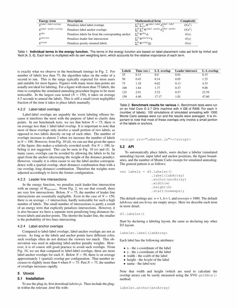
as the amount of energy the system possesses in order to jump overenergy barriers. This is visually represented in Fig. 5. Higher the tem-perature, the more likely we are to accepting configurations that have ahigh energy. Lower the temperature, the less likely we are to acceptingthese moves. In the case of T = 0, we go to the bottom of the near-est energy well. We start at a higher temperature in order to explorethe high dimensional energy surface. However, we slowly decreasethe temperature according to a schedule, also known as annealing thesystem. By doing so, we are focusing our search on deeper minima,and avoiding the higher energy configurations. The hope is that as thetemperature gets very low, we have found either the global minimumor a very low energy local minimum.
(a) High temperature
(b) Low temperature
Fig. 5. Simulated annealing at high and low temperatures. Theunlabeled vertical axis is energy. (a) At higher temperatures, we arenot likely to accept configurations that have a high energy. We startat a higher temperature term in order to explore the high dimensionalenergy surface. (b) At lower temperatures, we are less likely to accepthigh energy configurations. In the case of T = 0, we go to the bottomof the nearest energy well. As the simulation progresses, we slowlydecrease the temperature, also known as annealing the system. Bydoing so, we are focusing our search on deeper minima, and avoidingthe higher energy configurations. The hope is that as the temperaturegets very low, we have reached either the global minimum or a very lowenergy local minimum.
The protocol by which we lower the temperature is very importantto the resulting configuration. If the temperature is lowered very fast,often called “quenching”, the system can potentially get trapped in anearby local minima, resulting in a less than optimum final config-

uration. It is recommended that the system cools slowly rather thanrapidly [12], the reason being that we always want to keep the at orclose to the equilibrium at all temperatures. The most often used cool-ing schedules have been either linear
T (n) = T0αn, (6)
or exponential
T (n) = T0−βn, (7)
where T0 is the initial temperature, α , β are constants, and n is thenumber of steps taken [13].
Simulated annealing is often used with the Metropolis acceptancecriteria [11],
Pacc =
{e−∆E/kBT if ∆E > 0
1 if ∆E ≤ 0(8)
where Pacc is the probability of accepting a new label configuration,∆E is the change in energy of the system going from one configurationto another, kB is Boltzmann’s constant, and T is the system tempera-ture. In our case, we will denote temperature in reduced units of kB forsimplicity. The algorithm for simulated annealing is as follows.
while convergence not reached doattempt a move ν →ν ′ by translating or rotating labels;evaluate change in energy ∆E = Eν ′ −Eν ;if ∆E < 0 then
accept new configuration;else
generate random number ξ between 0 and 1;if ξ < e−∆E/T then
accept new configuration;else
reject configuration;end
enddecrease T according to schedule;
endAlgorithm 3: Simulated annealing
3 METHODS
3.1 Choice of algorithm
For any nontrivial labeling problem, the energy landscape will bevery high-dimensional (2N degrees of freedom) and rough. In orderto find a good label placement configuration, we have to avoid gettingtrapped in local minima. Therefore, global search algorithms are moresuited than local search algorithms. Out of the many global searchalgorithms available, simulated annealing is one of the more favoredalgorithms because of its simplicity, flexibility, and intuitive physicalbasis. It is also important for me to choose an algorithm that manypeople are familiar with, so that they can build on my work and addadditional functionality to suit their specific labeling preferences. Forthese reasons I have implemented the automatic label placement plu-gin using simulated annealing.
3.2 Incorporation within D3
My implementation is more generally a D3 simulated annealinggraphical layout, adapted for the problem of label placement. The en-ergy function in the layout corresponds to a particular set of graphicalrules that are described in the sections below. However, the users havethe option to define custom energy functions in order to suit individ-ual labeling preferences (details in Sec. 5.2). Furthermore, with ad-ditional changes, the simulated annealing tools within the plug-in canbe adapted for any optimization problem, such as drawing a node-linkdiagram.
3.3 Energy functionThe specific form of the energy function dictate the landscape of the
search space. Therefore, a carefully constructed energy function thatincorporates good labeling practices is crucial to the resulting labelingconfiguration. The energy function in the current implementation in-cludes terms for rules that I believe will appeal to a wide audience ofstudents, academics, and scientists in the industry setting. A tabularsummary of all the energy terms is shown in Table 1. In the follow-ing subsections I will describe in more detail the various terms in theenergy function and their corresponding labeling rules.
3.3.1 Label-label and label-feature overlapPerhaps the most important rule in label placement is to avoid label-
label and label-anchor overlaps. Overlaps not only hinder our abilityto decipher text but also compromise the overall aesthetics of the plot,giving it an unprofessional look. We use the following energy terms toaccount for overlaps
Eoverlap =N
∑i
N
∑j 6=i
W lab−labAlab−labi j +
N
∑i
N
∑j
W lab−ancAlab−anci j , (9)
where the first double sum represents the label-label overlaps and thesecond double sum represents the label-anchor overlaps. Ai j is thearea of the overlap between label i and label or anchor j, and W is theweight of the overlap energy penalties. In order to calculate overlaps,the labels as well as the anchor points have been approximated as rect-angles. The overlap term in the energy function is simply the area ofoverlap between the rectangles. This is illustrated in Fig. 6.
North BeachRussian Hill
Tenderloin
Russian Hill
(a) Label-label overlap (b) Label-anchor overlap
Fig. 6. Label-label and label-feature overlap. In order to calculateoverlaps, the labels and anchor points have been approximated as rect-angles. The overlap term in the energy function is simply the area ofoverlap between the rectangles. Overlap areas for (a) label-label and(b) label-anchor are colored in red.
3.3.2 Distance between feature and corresponding labelLabel positions closer to the corresponding point feature are pre-
ferred [4]. The further a label is positioned from its anchor point, themore difficult it is to detect correspondence. To account for this, weuse an energy penalty that is linear in the distance. The contribution toenergy corresponding to the label-feature distance is
Edist =N
∑i
W distdi, (10)
where di is the Euclidean distance between the label i and its corre-sponding anchor point, and W dist is the weight of the energy penalty.
3.3.3 Intersection of leader linesThe intersection of leader lines can hinder our ability to following aline to the end point, delaying our comprehension of the data. Theenergy penalty is simply a linear function of the number of leader lineintersections
E intersect =N
∑i
W intersect Ii, (11)
where I is a count of the total number of leader line intersections andW intersect is the weight of the energy penalty.

3.3.4 Label orientationIn addition to the more obvious rules of avoiding overlaps and lineintersections, Imhof also described a set of stylistic rules, includingthe relative desirability of label positions. This is shown in Fig. 3. Anenergy term was constructed in order to mimic these stylistic rules
Eorient =N
∑i
W orientQi, (12)
where Q = 1,2,3,or 4 is the quadrant preference index in Fig. 7 andW orient is the weight of the energy penalty. A pictorial representationof this energy function is shown in Fig. 7.
(0)(1)
(3)(2)
Fig. 7. Orientation bias. In Imhof’s seminal work on label rules, he setforth the relative desirability of label positions. This is shown in Fig. 3.An energy term was constructed in order to mimic these stylistic rules.Red is used to indicate presence of an energy penalty. Darker color andhigher number (quadrant preference index Q) represents higher energypenalty.
3.4 Monte Carlo movesIf we only use label translation moves, in theory, we are able to
sample the entire configuration space of label positions. However, thiswill not ensure the most efficient sampling protocol, as measured bythe time needed to find a sufficiently low energy minimum. This isbecause in general, it is more preferential for a label to be close to thecorresponding data point. If a label is at an optimum distance awayfrom its data point but in the wrong orientation, it would likely takemany translation moves for the label to shift to the right orientation,because in general translation a label changes its distance from thedata point. In this case, rotation moves will on average shift the labelto the right orientation faster. Therefore, to ensure both an ergodic andefficient sampling of the conformational space, we use a combinationof label translation and label rotation moves. These moves are shownin Fig. 8.
(a) Label translation
Union Square
(b) Label rotation
Union Square
Union Square
Union Square
Fig. 8. Monte Carlo moves. To ensure both an ergodic and efficientsampling of the conformational space, we use a combination of (a) labeltranslation and (b) label rotation moves.
3.5 Annealing scheduleAs mentioned before, the choice of good annealing schedule is veryimportant to the quality of the final configuration. For this problem Ichoose the popular linear cooling protocol [13]
T (n) = T0−T0
ntotn, (13)
where T0 is the initial temperature, n is the current number of MonteCarlo sweeps that have been implemented, and ntot is the total numberof Monte Carlo sweeps.
4 RESULTS
4.1 Sample label configurationsSample label configurations using the plugin are shown in Fig. 9.
In test runs, labels are initialized (Fig. 9a) such that the bottom leftcorner of the label is placed at the center of the anchor point. The re-sulting configurations are relatively insensitive to any reasonable labelinitialization schemes (i.e. labels are close to the anchor point). Forwell-separated labels, the most preferred position is the upper rightcorner, without any overlaps. This minimum can be easily found us-ing the implemented simulated annealing scheme (Fig. 9b). When twoanchor points are close together, most likely the two corresponding la-bels cannot be both in their most preferred position (Fig. 9c). In thiscase, one of the labels (Node 43) is in the preferred position while theother label (Node 16) is rotated and translated slightly in the verticaldirection. In a slightly different example (Fig. 9d), the algorithm findsa minima where the label for Node 7 is in its preferred position andthe label for Node 5 is rotated to the bottom with respect its anchor.
11/29/13 index.html
file://localhost/Users/evan/Dropbox/d3_layout/index.html 1/1
Start annealing
Node 0
Node 1
Node 2 Node 3
Node 4
Node 5
Node 6
Node 7
Node 8
Node 9
Node 10Node 11
Node 12
Node 13
Node 14Node 15
Node 16
Node 17
Node 18
Node 19
Node 20
Node 21
Node 22
Node 23
Node 24
11/29/13 index.html
file://localhost/Users/evan/Dropbox/d3_layout/index.html 1/1
Start annealing
Node 0
Node 1
Node 2
Node 3
Node 4
Node 5
Node 6
Node 7
Node 8
Node 9
Node 10
Node 11
Node 12
Node 13
Node 14 Node 15
Node 16
Node 17
Node 18
Node 19
Node 20
Node 21
Node 22
Node 23
Node 24
Node 25
Node 26
Node 27Node 28 Node 29
Node 30
Node 31
Node 32
Node 33
Node 34
Node 35
Node 36
Node 37
Node 38
Node 39
Node 40
Node 41
Node 42
Node 43Node 44
Node 45
Node 46
Node 47
Node 48
Node 49
11/29/13 index.html
file://localhost/Users/evan/Dropbox/d3_layout/index.html 1/1
Start annealing
Node 0
Node 1
Node 2
Node 3
Node 4
Node 5
Node 6
Node 7
Node 8
Node 9
Node 10
Node 11
Node 12
Node 13
Node 14
Node 15
Node 16
Node 17
Node 18
Node 19
Node 20
Node 21
Node 22
Node 23
Node 24
Node 25
Node 26
Node 27
Node 28
Node 29
Node 30
Node 31
Node 32
Node 33
Node 34
Node 35
Node 36
Node 37
Node 38
Node 39
Node 40
Node 41Node 42 Node 43
Node 44
Node 45
Node 46
Node 47
Node 48
Node 49
(a) (b)
(c) (d)
Fig. 9. Sample configurations. (a) Initialization: Labels are initializedsuch that the bottom left corner of the label is placed at the center ofthe anchor point. The final resulting configurations are relatively insen-sitive to reasonable label initialization schemes (i.e. labels are close tothe anchor point). (b) Global minima for individual, well-separated la-bels: For well-separated labels, the most preferred position is the upperright corner, without any overlaps. This minimum can be easily foundusing the implemented simulated annealing scheme. (c) Labels closetogether: When two anchor points are close together, most likely the twocorresponding labels cannot be both in their most preferred position. Inthis case, one of the labels (Node 43) is in the preferred position whilethe other label (Node 16) is rotated and translated slightly in the verticaldirection. (d) Labels close together: In this case, the algorithm finds aminima where label for Node 7 is in its preferred position and the labelfor Node 5 is rotated to the bottom with respect its anchor.
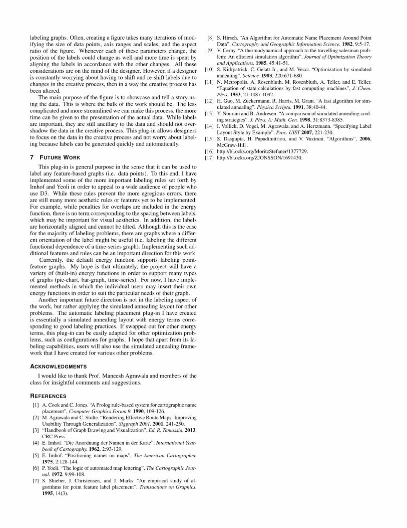
4.2 Benchmark resultsTo further evaluate the effectiveness of the plugin, benchmark sim-
ulations have been performed for different number of labels (N = 25,50,, 75, 100, 125, 150). They are summarized in Fig. 2. Results areevaluated based on run times, number of label-label overlaps, num-ber of label-anchor overlaps, and number of leader line intersections.These tests were run on an Intel Core i5 2.7 GHz machine with 4 GBof RAM. For each N (number of labels), 100 independent trials wereperformed, each for 1000 Monte Carlo sweeps1 The results shown inFig. 2 are averaged from the 100 trials. For each N, the final labelconfiguration of one run was saved and the snapshots are shown inFig. 10.
4.2.1 TimingOverall, the energy function is dominated by O(n2) terms, and so
we expect to see a quadratic dependence on the number of labels. This1One Monte Carlo sweep means that on average, each label is translated or
rotated once. To obtain the actual number of Monte Carlo steps taken, multiplythe number of sweeps by the number of labels N.
Energy term Description Mathematical form ComplexityE label−label overlap Penalizes label-label overlaps ∑
Ni ∑
Nj 6=i W
label−labelAlabel−labeli j O(n2)
E label−anchor overlap Penalizes label-anchor overlaps ∑Ni ∑
Nj W label−anchorAlabel−anchor
i j O(n2)
Edist Penalizes labels far from the corresponding anchor ∑Ni W dist di O(n)
E intersect Penalizes leader line intersection ∑Ni W intersect Ii O(n)
Eorient Penalizes poorly oriented labels ∑Ni W orient Qi O(n)
Table 1. Individual terms in the energy function. The terms in the energy function are based on label placement rules set forth by Imhof andYeoli [4, 5, 6]. Each term is multiplied with its own weighting term, which accounts for the relative importance of each term.
is exactly what we observe in the benchmark timings in Fig. 2. Fornumber of labels less than 75, the algorithm takes on the order of asecond to run. This is the range typically expected for most usersand suitable for most figures. Figures with many more data points areusually not ideal for labeling. For a figure with more than 75 labels, thetime to complete the simulated annealing procedure begins to be morenoticeable. In the largest case tested (N = 150), it takes on average4.5 seconds to anneal the labels. This is still a small (even negligible)fraction of the time it takes to place labels manually.
4.2.2 Label-label overlapsLabel-label overlaps are arguably the worst labeling offense be-
cause it interferes the most with the purpose of label to clarify datapoints. In our benchmark tests, we see that below N = 75, there ison average less than 1 label-label overlap. It is important to note thatmost of these overlaps only involve a small portion of two labels, asopposed to two labels directly on top of each other. The number ofoverlaps increase to almost 2 when we increase the number of labelsto N = 100. However, from Fig. 10 (d), we can see that given the spaceof the figure, this makes a relatively crowded result. For N > 100, la-beling is not suggested. This can be seen in Fig. 10 (e) and (f). Inmany cases, overlaps can be avoided by allowing the labels to be farapart from the anchor (decreasing the weight of the distance penalty).However, visually it is often easier to see the label anchor correspon-dence with a (partial overlap, short distance) combination than with a(no overlap, long distance) combination. Therefore the weights wereadjusted accordingly to favor the former configuration.
4.2.3 Leader line intersectionsIn the energy function, we penalize each leader-line intersection
with an energy of Wintersect . From Fig. 2, we see that overall, thereare very few intersections. Below, N = 75, the number of leader lineintersections are essentially negligible. Even in the case of N = 150,there is on average ∼1 intersection, hardly noticeable for such a highnumber of labels. The small number of intersections is partly a resultof an energy term that explicitly penalizes intersections. However, itis also because we have a separate term penalizing long distances be-tween labels and anchor points. The shorter the leader line, the smalleris the probability of two lines intersecting.
4.2.4 Label-anchor overlapsCompared to label-label overlaps, label-anchor overlaps are not as
severe. As long as the labels and anchor points have different color,such overlaps often do not distract the viewers too much. This ob-servation was used in adjusting label-anchor penalty weights. How-ever, it is of course still good practice to avoid such overlaps. FromFig. 10, we see that compared to label-label overlaps, there are morelabel-anchor overlaps for each N. Below N = 50, there is on averageapproximately 1 (partial) overlap per configuration. That number in-creases to slightly more than 4 when N = 75. Past N = 75, the numberof overlaps increases rapidly.
5 USAGE
5.1 InstallationTo use the plug-in, first download labeler.js. Then include the plug-
in within the relevant .html file with:
Labels Time (sec.) L-L overlap Leader intersect. L-A overlap25 0.13 0.0 0.01 0.1550 0.45 0.14 0.05 1.2575 1.10 0.62 0.13 4.35100 1.84 1.77 0.37 9.88125 2.91 5.52 0.57 23.59150 4.40 17.17 1.01 47.60
Table 2. Benchmark results for various N. Benchmark tests were runon an Intel Core i5 2.7 GHz machine with 4 GB of RAM. For each N(number of labels), 100 simulations of simulated annealing with 1000Monte Carlo sweeps were run and the results were averaged. It is im-portant to note that most of these overlaps only involve a small portionof the labels or anchors.
<script src="labeler.js"></script>
5.2 APITo automatically place labels, users declare a labeler (simulated
annealing) layout, input label and anchor positions, the figure bound-aries, and the number of Monte Carlo sweeps for simulated annealing.The general pattern is as follows:
var labels = d3.labeler().label(labArray).anchor(ancArray).width(w).height(h).start(nsweeps);
The default settings are: w = 1, h = 1, and nsweeps = 1000. The defaultlabArray and ancArray are empty arrays. Here we describe each termin more detail.
d3.labeler()
Start by declaring a labeling layout, the same as declaring any otherD3 layout.
labeler.label(labArray)
Each label has the following attributes:
• x - the x-coordinate of the label• y - the y-coordinate of the label• width - the width of the label• height - the height of the label• name - the label text
Note that width and height (which are used to calculate theoverlap areas) can be easily measured using the SVG getBBox()method.
labeler.anchor(ancArray)

11/29/13 index.html
file://localhost/Users/evan/Dropbox/d3_layout/index.html 1/1
Start annealing
Node 0
Node 1
Node 2
Node 3
Node 4
Node 5
Node 6
Node 7
Node 8
Node 9
Node 10
Node 11
Node 12
Node 13
Node 14
Node 15
Node 16
Node 17
Node 18
Node 19
Node 20
Node 21
Node 22
Node 23
Node 24
11/29/13 index.html
file://localhost/Users/evan/Dropbox/d3_layout/index.html 1/1
Start annealing
Node 0Node 1
Node 2
Node 3
Node 4
Node 5
Node 6
Node 7
Node 8
Node 9Node 10
Node 11
Node 12
Node 13
Node 14
Node 15
Node 16
Node 17
Node 18
Node 19
Node 20
Node 21
Node 22
Node 23
Node 24
Node 25
Node 26
Node 27
Node 28
Node 29
Node 30
Node 31
Node 32
Node 33
Node 34
Node 35 Node 36
Node 37
Node 38
Node 39
Node 40
Node 41
Node 42
Node 43
Node 44
Node 45Node 46
Node 47
Node 48
Node 49
11/29/13 index.html
file://localhost/Users/evan/Dropbox/d3_layout/index.html 1/1
Start annealing
Node 0
Node 1
Node 2
Node 3
Node 4
Node 5
Node 6
Node 7Node 8
Node 9Node 10
Node 11
Node 12
Node 13
Node 14
Node 15 Node 16
Node 17
Node 18
Node 19
Node 20Node 21
Node 22
Node 23
Node 24
Node 25
Node 26
Node 27
Node 28
Node 29
Node 30
Node 31
Node 32
Node 33
Node 34
Node 35
Node 36
Node 37
Node 38
Node 39
Node 40
Node 41
Node 42
Node 43
Node 44
Node 45
Node 46
Node 47
Node 48
Node 49
Node 50
Node 51
Node 52
Node 53
Node 54Node 55
Node 56
Node 57
Node 58
Node 59
Node 60
Node 61
Node 62Node 63
Node 64
Node 65
Node 66
Node 67
Node 68
Node 69
Node 70
Node 71
Node 72
Node 73
Node 74
(a) (b) (c)11/29/13 index.html
file://localhost/Users/evan/Dropbox/d3_layout/index.html 1/1
Start annealing
Node 0Node 1
Node 2
Node 3
Node 4
Node 5
Node 6
Node 7
Node 8
Node 9
Node 10
Node 11Node 12
Node 13
Node 14
Node 15
Node 16
Node 17
Node 18
Node 19Node 20
Node 21
Node 22
Node 23
Node 24
Node 25
Node 26
Node 27
Node 28Node 29
Node 30
Node 31
Node 32
Node 33
Node 34Node 35
Node 36
Node 37
Node 38
Node 39
Node 40
Node 41
Node 42
Node 43
Node 44
Node 45
Node 46Node 47
Node 48
Node 49
Node 50
Node 51
Node 52
Node 53
Node 54
Node 55
Node 56
Node 57
Node 58
Node 59
Node 60
Node 61
Node 62
Node 63
Node 64
Node 65
Node 66Node 67
Node 68
Node 69
Node 70
Node 71
Node 72
Node 73Node 74
Node 75
Node 76
Node 77
Node 78
Node 79
Node 80
Node 81Node 82
Node 83
Node 84
Node 85
Node 86
Node 87
Node 88
Node 89
Node 90
Node 91
Node 92
Node 93
Node 94
Node 95
Node 96Node 97
Node 98
Node 99
11/29/13 index.html
file://localhost/Users/evan/Dropbox/d3_layout/index.html 1/1
Start annealing
Node 0
Node 1
Node 2
Node 3
Node 4
Node 5
Node 6
Node 7
Node 8
Node 9Node 10
Node 11
Node 12
Node 13
Node 14
Node 15
Node 16
Node 17
Node 18
Node 19
Node 20
Node 21
Node 22
Node 23
Node 24
Node 25
Node 26
Node 27
Node 28
Node 29
Node 30
Node 31
Node 32
Node 33
Node 34Node 35
Node 36
Node 37
Node 38
Node 39
Node 40
Node 41
Node 42
Node 43Node 44
Node 45
Node 46
Node 47
Node 48
Node 49
Node 50
Node 51
Node 52
Node 53
Node 54
Node 55
Node 56
Node 57
Node 58
Node 59
Node 60
Node 61
Node 62Node 63
Node 64
Node 65
Node 66
Node 67
Node 68
Node 69
Node 70
Node 71
Node 72Node 73Node 74
Node 75Node 76
Node 77
Node 78 Node 79
Node 80
Node 81Node 82
Node 83
Node 84
Node 85 Node 86
Node 87
Node 88
Node 89
Node 90
Node 91
Node 92
Node 93
Node 94
Node 95
Node 96
Node 97
Node 98
Node 99
Node 100
Node 101
Node 102Node 103
Node 104
Node 105
Node 106
Node 107
Node 108
Node 109
Node 110Node 111
Node 112
Node 113
Node 114
Node 115
Node 116
Node 117
Node 118
Node 119
Node 120
Node 121
Node 122
Node 123
Node 124
11/29/13 index.html
file://localhost/Users/evan/Dropbox/d3_layout/index.html 1/1
Start annealing
Node 0
Node 1
Node 2
Node 3
Node 4
Node 5
Node 6 Node 7
Node 8
Node 9
Node 10
Node 11
Node 12
Node 13
Node 14
Node 15
Node 16
Node 17Node 18
Node 19
Node 20
Node 21
Node 22
Node 23
Node 24Node 25
Node 26
Node 27
Node 28
Node 29
Node 30
Node 31
Node 32
Node 33
Node 34Node 35
Node 36
Node 37
Node 38
Node 39
Node 40
Node 41
Node 42
Node 43
Node 44
Node 45
Node 46
Node 47
Node 48
Node 49
Node 50 Node 51Node 52
Node 53
Node 54Node 55
Node 56
Node 57
Node 58
Node 59
Node 60
Node 61
Node 62
Node 63
Node 64
Node 65
Node 66
Node 67
Node 68
Node 69
Node 70
Node 71
Node 72
Node 73
Node 74
Node 75
Node 76
Node 77
Node 78
Node 79
Node 80
Node 81
Node 82
Node 83
Node 84
Node 85
Node 86
Node 87
Node 88Node 89
Node 90
Node 91
Node 92
Node 93Node 94
Node 95
Node 96
Node 97
Node 98
Node 99
Node 100
Node 101
Node 102
Node 103
Node 104
Node 105
Node 106
Node 107
Node 108
Node 109
Node 110
Node 111
Node 112
Node 113
Node 114
Node 115Node 116
Node 117
Node 118Node 119
Node 120
Node 121
Node 122
Node 123
Node 124
Node 125
Node 126Node 127
Node 128
Node 129
Node 130
Node 131
Node 132Node 133
Node 134
Node 135
Node 136
Node 137
Node 138
Node 139
Node 140
Node 141
Node 142
Node 143
Node 144
Node 145
Node 146
Node 147
Node 148
Node 149
(d) (e) (f)
FIG. 1: Renormalization of the material properties of a flat membrane due to volume excluding spherical proteins adhered to its surface.(a) h|hq |2i spectrum of the membrane height fluctuations around its flat state versus the corresponding mode q without adhered proteins(upper) and including adhered proteins (lower). The e↵ective bending rigidity and surface tension are determined by fitting the smalland long wavelength fluctuation regime respectively (solid line). The dashed line for comparison corresponds to a case without adheredproteins and vanishing surface tension. (b) Renormalization of the bending rigidity and surface tension (inset) as a function of packingfraction of adhered proteins for = 10kBT (triangles) and 20kBT (circles). Dashed and solid lines are the theoretical expectations. (c)Wavelength dependent instability regimes versus packing fraction of adhered proteins. For low packing fractions of adhered proteins, themembrane fluctuations around the flat state are stable. At intermediate packing fractions, the large wavelength modes become unstable.At fixed projected area and fluctuating but finite membrane area, these fluctuations are still constraint around the flat state. However, foreven higher packing fractions, the membrane fluctuations around the flat state become unstable at all wavelengths. As a consequence asmall and highly curved membrane protrusion is observed.
(a) (b) (c)
(d) (e) (f)
Fig. 10. Snapshots of the final label configuration for various number of labels (N). (a) N = 25 (b) N = 50 (c) N = 75 (d) N = 100 (e) N = 125(f) N = 150.
Each anchor has the following attributes:
• x - the x-coordinate of the anchor• y - the y-coordinate of the anchor• r - the anchor radius
labeler.width(w)labeler.height(h)
The width and height are used to set the boundary conditions so that la-bels do not go outside the width and height of the figure. More specifi-cally, Monte Carlo moves in which the labels cross the boundaries arerejected. If they are not specified, both the width and height default to1.
labeler.start(nsweeps)
Finally, we specify the number of Monte Carlo sweeps for the opti-mization and run the simulated annealing procedure. The default fortextitnsweeps is 1000. Note that one Monte Carlo sweep means that onaverage, each label is translated or rotated once. To obtain the actualnumber of Monte Carlo steps taken, multiply the number of sweeps bythe number of labels.
labeler.alt_energy(user_defined_energy)
This function is constructed for expert users. The quality of the con-figuration is closely related to the energy function. The default en-ergy function includes general labeling preferences and is suggestedfor most users. However, a user may wish to define his or her ownenergy function to suit individual preferences.
energy = function(idx, labArray, ancArray) {var ener = 0;// insert interaction energies herereturn ener;
}
The newly constructed function must take as input an integer idx, anarray of labels labArray, and an array of anchors ancArray. This func-tion must also return an energy term that should correspond to theenergy of a particular label, namely labArray[idx]. One may wish cal-culate an energy of interaction for labArray[idx] with all other labelsand anchors.
labeler.alt_schedule(user_defined_schedule)
Similarly, an expert user may wish to include a custom cooling sched-ule used in the simulated annealing procedure. The default coolingschedule is linear.
schedule = function(currT, initT, nsweeps) {// insert user-defined schedule herereturn updatedT;
}
This function takes as input the current simulation temperature currT,the initial temperature initT, and the total number of sweeps nsweepsand returns the updated temperature updatedT. The user defined func-tions can be included as follows:
var labels = d3.labeler().label(label_array).anchor(anchor_array).width(w).height(h).alt_energy(ener).alt_schedule(schedule).start(nsweeps);
6 DISCUSSION AND CONCLUSION
The intent of this work is to implement a good algorithm for au-tomatic label placement in D3 and save designers time from manually
labeling graphs. Often, creating a figure takes many iterations of mod-ifying the size of data points, axis ranges and scales, and the aspectratio of the figure. Whenever each of these parameters change, theposition of the labels could change as well and more time is spent byaligning the labels in accordance with the other changes. All theseconsiderations are on the mind of the designer. However, if a designeris constantly worrying about having to shift and re-shift labels due tochanges in the creative process, then in a way the creative process hasbeen altered.
The main purpose of the figure is to showcase and tell a story us-ing the data. This is where the bulk of the work should be. The lesscomplicated and more streamlined we can make this process, the moretime can be given to the presentation of the actual data. While labelsare important, they are still ancillary to the data and should not over-shadow the data in the creative process. This plug-in allows designersto focus on the data in the creative process and not worry about label-ing because labels can be generated quickly and automatically.
7 FUTURE WORK
This plug-in is general purpose in the sense that it can be used tolabel any feature-based graphs (i.e. data points). To this end, I haveimplemented some of the more important labeling rules set forth byImhof and Yeoli in order to appeal to a wide audience of people whouse D3. While these rules prevent the more egregious errors, thereare still many more aesthetic rules or features yet to be implemented.For example, while penalties for overlaps are included in the energyfunction, there is no term corresponding to the spacing between labels,which may be important for visual aesthetics. In addition, the labelsare horizontally aligned and cannot be tilted. Although this is the casefor the majority of labeling problems, there are graphs where a differ-ent orientation of the label might be useful (i.e. labeling the differentfunctional dependence of a time-series graph). Implementing such ad-ditional features and rules can be an important direction for this work.
Currently, the default energy function supports labeling point-feature graphs. My hope is that ultimately, the project will have avariety of (built-in) energy functions in order to support many typesof graphs (pie-chart, bar-graph, time-series). For now, I have imple-mented methods in which the individual users may insert their ownenergy functions in order to suit the particular needs of their graph.
Another important future direction is not in the labeling aspect ofthe work, but rather applying the simulated annealing layout for otherproblems. The automatic labeling placement plug-in I have createdis essentially a simulated annealing layout with energy terms corre-sponding to good labeling practices. If swapped out for other energyterms, this plug-in can be easily adapted for other optimization prob-lems, such as configurations for graphs. I hope that apart from its la-beling capabilities, users will also use the simulated annealing frame-work that I have created for various other problems.
ACKNOWLEDGMENTS
I would like to thank Prof. Maneesh Agrawala and members of theclass for insightful comments and suggestions.
REFERENCES
[1] A. Cook and C. Jones. “A Prolog rule-based system for cartographic nameplacement”, Computer Graphics Forum 9. 1990, 109-126.
[2] M. Agrawala and C. Stolte. “Rendering Effective Route Maps: ImprovingUsability Through Generalization”, Siggraph 2001. 2001, 241-250.
[3] “Handbook of Graph Drawing and Visualization”, Ed. R. Tamassia. 2013,CRC Press.
[4] E. Imhof. “Die Anordnung der Namen in der Karte”, International Year-book of Cartography. 1962, 2:93-129.
[5] E. Imhof. “Positioning names on maps”, The American Cartographer.1975, 2:128-144.
[6] P. Yoeli. “The logic of automated map lettering”, The Cartographic Jour-nal. 1972, 9:99-108.
[7] S. Shieber, J. Christensen, and J. Marks. “An empirical study of al-gorithms for point feature label placement”, Transactions on Graphics.1995, 14(3).
[8] S. Hirsch. “An Algorithm for Automatic Name Placement Around PointData”, Cartography and Geographic Information Science. 1982, 9:5-17.
[9] V. Cerny. “A thermodynamical approach to the travelling salesman prob-lem: An efficient simulation algorithm”, Journal of Optimization Theoryand Applications. 1985, 45:41-51.
[10] S. Kirkpatrick, C. Gelatt Jr., and M. Vecci. “Optimization by simulatedannealing”, Science. 1983, 220:671-680.
[11] N. Metropolis, A. Rosenbluth, M. Rosenbluth, A. Teller, and E. Teller.“Equation of state calculations by fast computing machines”, J. Chem.Phys. 1953, 21:1087-1092.
[12] H. Guo, M. Zuckermann, R. Harris, M. Grant. “A fast algorithm for sim-ulated annealing”, Physica Scripta. 1991, 38:40-44.
[13] Y. Nourani and B. Andresen. “A comparison of simulated annealing cool-ing strategies”, J. Phys. A: Math. Gen. 1998, 31:8373-8385.
[14] I. Vollick, D. Vogel, M. Agrawala, and A. Hertzmann. “Specifying LabelLayout Style by Example”, Proc. UIST 2007, 221-230.
[15] S. Dasgupta, H. Papadimitriou, and V. Vazirani. “Algorithms”, 2006,McGraw-Hill .
[16] http://bl.ocks.org/MoritzStefaner/1377729.[17] http://bl.ocks.org/ZJONSSON/1691430.