A D-optimal design for estimation of

parameters of an exponential-linear growth

curve of nanostructures

Li Zhu†, Tirthankar Dasgupta†, Qiang Huang‡

†Department of Statistics,

Harvard University, Cambridge, MA 02138

‡Department of Industrial and Systems Engineering

University of Southern California, Los Angeles, CA 90089

Abstract

We consider the problem of determining an optimal experimental design for esti-

mation of parameters of a class of complex curves characterizing nanowire growth that

is partially exponential and partially linear. Locally D-optimal designs for some of

the models belonging to this class are obtained by using a geometric approach. Fur-

ther, a Bayesian sequential algorithm is proposed for obtaining D-optimal designs for

models with a closed-form solution, and for obtaining efficient designs in situations

where theoretical results cannot be obtained. The advantages of the proposed algo-

rithm over traditional approaches adopted in recently reported nano-experiments are

demonstrated using Monte-Carlo simulations. The computer code implementing the

sequential algorithm is available as supplementary material.

KEY WORDS: Non-linear model, Bayesian design, Sequential algorithm.

1

1 Introduction

Nanostructured materials and processes have been estimated to increase their market impact

to about $340 billion per year in the next 10 years. However, high cost of processing has

been a major barrier in transferring the fast-developing nanotechnology from laboratories to

industry applications. The process yield of current nano devices being very poor (typically

10% or less), there is a need for process improvement methodologies in nanomanufacturing.

For this purpose, it is important to understand the growth mechanisms of nanostructures

better through controlled experimentation. Statistical design of experiments are therefore

expected to play an important role in this area (Dasgupta et al. 2008, Lu et al. 2009).

Let Y (t) denote the value of a quality characteristic (e.g., weight of nanostructures grown,

see Huang et al. 2011) of a nanostructure synthesized using the vapor-liquid-solid (VLS)

process at time t at a specific location. Huang et al. (2011) experimentally investigated six

weight kinetics models to study weight change of nanostructures over time. In this paper we

shall consider three of these models, that are of the form

Y (t) = gθ(t) + ϵ, t > 0, (1)

where gθ(·) is a parametric function of time t, θ represents a parameter vector, and the error

terms (ϵ) are independently and identically distributed (iid) as N(0, σ2). The iid assumption

is justified by the fact that an experimental unit (a substrate on which nanostructures are

grown) can generate only a single data point at the time it is taken out of the furnace and

examined under the microscope. The three models differ with respect to the specification

for gθ(·). The first model has a pure exponential growth function where

gθ(t) = α1e−α2/t. t > 0. (2)

In all future discussions, we shall refer to model (1) with gθ(·) defined by (2) as model M1.

The other two models, henceforth referred to as models M3 and M4 respectively (model

M2 will be introduced later), are characterized by a exponential-linear change-point growth

function:

gθ(t) =

α1e−α2

t , tmin ≤ t < t0

a+ bt, t0 ≤ t ≤ tmax,, (3)

2

where α1 > 0, α2 > 0, b > 0; tmin and tmax denote respectively the (known) earliest and

latest time points at which it is feasible to conduct a trial; and t0 is an unknown time such

that the length L(t0) of a nanostructure at time t0 is the diffusion length defined in growth

kinetics. The model, without any constraints on the function gθ(t), contains five parameters

α1, α2, a, b and t0, other than the variance parameter σ2. Models M3 and M4 differ by the

fact that the former has a strong assumption of continuity of gθ(t) and also its first derivative

g′θ(t) at t0, whereas the latter relaxes the assumption of continuity of g′θ(t), and only assumes

continuity of gθ(t) at t0. It can easily be seen (Section 2) that models M3 and M4 can be

reduced to three and four parameter models respectively.

Based on their experimental results, Huang et al. (2011) identified model M4 as the most

appropriate model among the three. They used an experimental strategy (i.e., selection of

the time points t ∈ [tmin, tmax] at which the growth was observed) which utilized the prior

knowledge that the change-point t0 was more likely to occur early in the growth process.

Thus, instead of selecting equispaced points within tmin = 0.5 minutes and tmax = 210

minutes, they chose 19 time points that were more or less equally-spaced on a log-scale.

Three replicates of the basic experiment were conducted.

However, this experimental strategy of conducting 57 experimental runs to estimate the

parameters of the model was considered too expensive (gold is usually used as a catalyst)

and time consuming (terminating the process at a certain time t, taking out the substrate

from the furnace, and measuring the weight using a high-precision microbalance). Naturally,

scientists are interested in coming up with an efficient experimentation strategy that would:

(i) allow available scientific knowledge to be incorporated into the experimental design, (ii)

involve as few trials as possible, and yet (iii) allow precise estimation of model parameters.

In this article, we derive a locally D-optimal experimental design for the above estimation

problem using a geometric approach and also propose a sequential Bayesian strategy that

converges to the locally D-optimal design at the true parameter values.

A locally D-optimal design for model M1 (in a slightly different form) was derived by

Mukhopadhyay and Haynes (1995). In this paper we shall derive locally D-optimal designs

for models M3 and M4. To do this, we will introduce another model M2, which has the same

functional form of gθ(·) as M3 and M4 given by (3), but assumes that the change point t0 is

known and hence does not need to be estimated. Note that model M2 is not of any practical

3

interest; we introduce it merely to explain the geometrical argument with a better logical

flow that starts with a two-dimensional problem.

There has been some recent work on Bayesian D-optimal design with change points

(Atherton et al 2009). However, our problem does not have the typical “on-line” nature

associated with the problem considered by Atherton et al. (2009), and most change-point

problems. Typically, in such problems the experimenter continues to observe the process

over time and has to decide when a change has occurred in the generative parameters of the

data sequence. As explained earlier, this is not the case in our experimental setting, which

can be considered “off-line” in the sense that an experimental unit can generate only a single

data point at the time. Consequently, the assumptions used in Atherton et al. (2009) (pre-

specified distance d between any two design points and no replicated observation) do not

hold in the current problem. There has also been some recent work on D-optimal designs

for spline models (Biedermann et al. 2011).

The paper is organized as follows. In the following section, we give an overview of locally

D-optimal designs and state the work done for model M1. In Section 3, we describe the

geometric approach for obtaining D-optimal designs, and use it to derive locally D-optimal

designs for models M2 and M3. Since a D-optimal design for a non-linear model like (3)

will involve the true values of the parameters, in Section 4 we suggest a sequential Bayesian

strategy to obtain designs that are expected to converge to the true D-optimal design and

use it to derive a design for model M4. In Section 5, we re-visit the experimental strategy

adopted by Huang et al. (2011) for estimation of parameters of model M4 and demonstrate

how the proposed strategy can help reduce the number of experimental runs. Section 6

presents some concluding remarks and opportunities for future work.

2 Information matrix and locally D-optimal designs

As mentioned in Section 1, the objective is to design an experiment which will help us

estimate the parameter vector θ with a reasonably high degree of precision. We need to

determine at which time points t the trials should be conducted. Mathematically speaking,

the design space X is the closed interval [tmin, tmax]. A design ξ can be defined as a probability

4

measure on X of the form

ξ =

t1 . . . tr

w1 . . . wr

,

with distinct support points t1, . . . , tr in X and weights w1, . . . , wr which satisfy 0 < wi ≤ 1

for all i = 1, . . . , r and∑r

i=1wi = 1, where r is a positive integer. Such a design is typically

referred to as an approximate design. If the number of runs n is pre-specified, and all the

weights wi are integral multipliers of 1/n, then ξ is called an exact design with n observations.

In this paper, we consider the problem of finding approximate optimal designs for models

M2,M3 and M4.

Finding such an optimal design means selecting a measure ξ that will optimize a certain

function associated with the Fisher Information Matrix I(θ, ξ) for the model under consider-

ation. Specifically, here we consider a D-optimal design (Atkinson, Donev and Tobias 2007;

Federov 1972), which is obtained by maximizing the determinant of I(θ, ξ) over the possible

designs ξ. In other words, the optimal design measure ξ∗ will be such that

det

∫I(θ, ξ∗)ξ∗(dt) ≥ det

∫I(θ, ξ)ξ(dt), (4)

for all ξ ∈ Ξ.

We now derive the information matrices for the models M1 through M4.

Information matrix for model M1: For model M1, the Fisher information matrix at a

single design point t is:

I(θ, ξt) =1

σ2e−2α2/t

1 −α1

t

−α1

t

α21

t2

,

where ξt denotes a one-point probability measure with support t. The above matrix can be

expressed in the form 1σ2v1v

′1, where v′

1 = e−α2t (1,−α1

t).

Information matrices for models M2 and M3: For models M2 and M3, using the

continuity and differentiability of gθ(t) at t = t0, it is easy to see that a = α1(1−α2/t0)e−α2/t0

and b = (α1α2)/t20e

−α2/t0 , so that model M2 is essentially a two-parameter model with

θ = (α1, α2), whereas model M3 has three unknown parameters α1, α2 and t0.

5

For model M2, the Fisher information matrix can be expressed in the form 1σ2v2v

′2, where

v′2 =

e−α2t (1,−α1

t), t < t0

e−α2

t0

(1− α2

t0+ α2t

t20,−α1

t0(2− α2

t0− t

t0+ α2t

t20)). t ≥ t0

(5)

Similarly, the information matrix for model M3 can be expressed as 1σ2v3v

′3, where

v′3 =

e−α2t

(1,−α1

t, 0), t < t0

e−α2

t0

(1− α2

t0+ α2t

t20,−α1

t0(2− α2

t0− t

t0+ α2t

t20), α1α2

t20

(2− α2

t0− 2t

t0+ α2t

t20

)). t ≥ t0

(6)

Information matrix for model M4: Since for model M4 the first derivative of the function

gθ(t) is no longer continuous at t0, we have an extra slope parameter b. The intercept a of

the linear part can be obtained from a = α1e−α2

t0 − bt0.

In this model, the information matrix can be expressed in the form 1σ2v4v

′4, where

v′4 =

e−α2t (1,−α1

t, 0, 0), t < t0(

e−α2

t0 ,−α1

t0e−α2

t0 , α1α2

t20e−α2

t0 − b, t− t0

). t ≥ t0

(7)

Note that in this case, v4 is no longer continuous at time t0.

The above representation of the information matrix I in the form vv′ will be seen to

be very useful in derivation of the locally D-optimal design as well as the sequential design.

Note that since models M1 to M4 are intrinsically non-linear, the Fisher information matrix

in all three cases depends on the model parameters. Therefore the optimal design ξ∗ that

maximizes the D-optimality criterion det∫I(θ, ξ)ξ(dt) will actually be a locally D-optimal

design (Chernoff 1953) at θ. Moreover, since dispersion parameter σ2 serves as scalar variable

for information matrices for M1 to M4, it will not affect the optimization to obtain the locally

D-optimal design.

Proceeding in lines with the proof of Theorem 1 in Mukhopadhyay and Haines (1995)

(see Appendix), the following Theorem can be established.

Theorem 1. The locally D-optimal design for model M1 is a balanced two points design with

unique support at the points t∗1, t∗2, where t∗2 = tmax, and t∗1 = max

(α2t∗2α2+t∗2

, tmin

).

6

3 A geometric approach to D-Optimal designs and its

application to models M2 through M4

The geometric interpretation of D-optimal designs has a long history. Silvey (1972), Sibson

(1972), Silvey and Titterington (1973), Ford et al. (1992), Haines (1993) and Vandenberghe

et al. (1998) have studied the geometric properties of D-optimal designs, which actually

follow from the dual of the optimization problem given by (4).

Let θ be a vector of k unknown parameters and suppose the k × k information matrix I

can be expressed in the form vv′, where v is a member of a compact subset V of Rk. Then,

the definition of D-optimality described earlier in Section 2 can be extended as follows (Tit-

terington 1975): the design that maximizes log det∫V vv

′ξ(dv) is D-optimal for estimating θ.

Sibson (1972) showed that the resulting information matrix defines the ellipsoid of smallest

volume, centered at the origin, that contains V . It is also known (Vandenberghe et al. 1998)

that the points that lie on the boundary of the minimum volume ellipsoid are the only ones

that have non-zero mass. In other words, the points on the boundary of the ellipsoid will be

the only support points of the design.

Note that, all the D-optimal designs derived in this Section will actually be locally D-

optimal designs; however, for convenience, we shall drop the word “locally” and simply refer

to them as D-optimal designs.

3.1 D-optimal design for model M2

Consider the growth function gθ(t) given by (3) with α1 = 10, α2 = 1.2, tmin = 5, tmax = 40

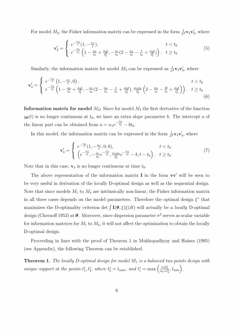
and t0 = 5. The left panel of Figure 1 shows the plot of the function gθ(t) (as a line) and

the response Y (t) (as points scattered around the line) given by (1) with σ = 0.5. For this

model, it follows from (5) that v = v2 = (v12, v22) represents a two dimensional vector in the

compact set V2 = {(v12(t), v22(t)) : tmin ≤ t ≤ tmax}, where

v12(t) =

e−α2t , t < t0

e−α2

t0

(1− α2

t0+ α2t

t20

), t ≥ t0

, v22(t) =

−α1

te−

α2t , t < t0

−α1

t0e−α2

t0

(2− α2

t0− t

t0+ α2t

t20

). t ≥ t0

.

The right panel of Figure 1 shows all the points in the set V2 defined above and the

minimum volume ellipse centered at the origin that contains all these points. The locus of

7

0 10 20 30 40

05

1015

20

t

g(t)

and

y(t

)

t0

−3 −2 −1 0 1 2 3

−5

05

v21

v 22

t0

tmax

Figure 1: Response function (left panel) and Minimum volume ellipse that contains V (right

panel) for Model M2 with α1 = 10, α2 = 1.2, σ = 0.5, tmin = 0.1, tmax = 40 and t0 = 5.

v2 is a straight line for t ≥ t0 with slope (α1/α2)(1 − α2/t0), which is positive for α2 < t0,

parallel to the horizontal axis if α2 = t0, and negative otherwise. It is easy to see that

dv11(t)/dt > 0, which indicates that the line has to move away from the origin. It follows

that for all values of the parameters, the minimum volume ellipse must touch only two points

on the curve; one of them is (x1, y1) = (v12(tmax), v22(tmax)), which lies at one extreme of the

curve. It is obvious that the second point will be of the form (x2, y2) = (v12(t), v22(t)) for

some t ≤ t0. Minimizing the volume of the ellipsoid passing through (x1, y1) and (x2, y2)

with respect to t, we obtain the second support point of the D-optimal design and hence

arrive at the following Theorem (detailed proof in Appendix):

Theorem 2. Define

τ =α2

1− α2(tmax−2t0)t0−α2(tmax−t0)

t0(t20+α2(tmax−t0))

. (8)

The D-optimal design for model M2 is a balanced two-point design with unique support at

t∗1, t∗2, where

t∗2 = tmax and t∗1 = max (τ, tmin) .

Remark: Clearly, as tmax → t0, model M2 tends to model M1 with maximum feasible time

8

t0. Note that

limtmax→t0

t∗1 = max

(α2t0

α2 + t0, tmin

),

which shows that the limiting value of t∗1 as tmax → t0 is the same as t∗1 for model M1. Thus,

Theorem 1 can be deduced as a special case of Theorem 2.

3.2 D-optimal design for model M3

0.0 0.5 1.0 1.5 2.0 2.5

−6

−5

−4

−3

−2

−1

0

−4

−2

0

2

4

6

8

v31

v 32v 33 tmax

t0

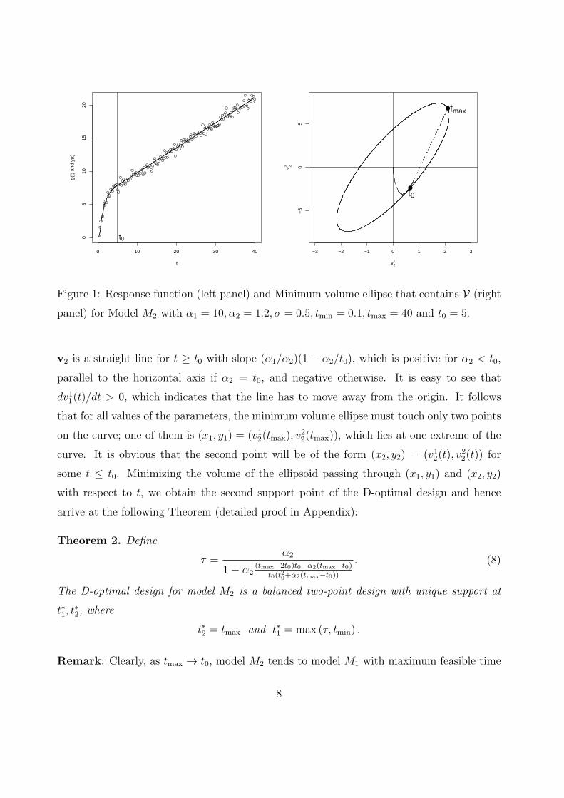
Figure 2: Plot of candidate points in V3 for Model M3 with α1 = 10, α2 = 1.2, tmin =

0.1, tmax = 40.

Now we consider the case when the change-point t0 is unknown. For this model, v = v3 =

(v13, v23, v

33) represents a three-dimensional vector in the compact set V3 = {(v13(t), v23(t), v33(t)) :

tmin ≤ t ≤ tmax}, where vj3(t), j = 1, 2, 3 represent the components of v3 given by (6). Note

that they are different for t < t0 and t ≥ t0. Figure 2 shows all the points in the set V3 defined

above. The points lie on a curve in the X − Y plane for t < t0, and then fall on a straight

line in the 3-D space till t = tmax. In this case, the minimum volume ellipsoid must touch

three of the points in V3, one of which has to be (v13(tmax), v23(tmax), v

33(tmax)), i.e., the point

corresponding to t = tmax. It is not difficult to see that if the minimum volume ellipsoid is

made to pass through this point, then the maximization problem reduces to maximization of

9

the projection of the ellipsoid on the X − Y plane. Consequently, we arrive at the following

Theorem (detailed proof in Appendix):

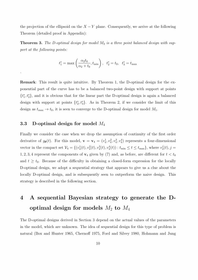
Theorem 3. The D-optimal design for model M3 is a three point balanced design with sup-

port at the following points:

t∗1 = max

(α2t0

α2 + t0, tmin

), t∗2 = t0, t∗3 = tmax

.

Remark: This result is quite intuitive. By Theorem 1, the D-optimal design for the ex-

ponential part of the curve has to be a balanced two-point design with support at points

{t∗1, t∗2}, and it is obvious that for the linear part the D-optimal design is again a balanced

design with support at points {t∗2, t∗3}. As in Theorem 2, if we consider the limit of this

design as tmax → t0, it is seen to converge to the D-optimal design for model M1.

3.3 D-optimal design for model M4

Finally we consider the case when we drop the assumption of continuity of the first order

derivative of gθ(t). For this model, v = v4 = (v14, v24, v

34, v

44) represents a four-dimensional

vector in the compact set V4 = {(v14(t), v24(t), v34(t), v44(t)) : tmin ≤ t ≤ tmax}, where vj4(t), j =

1, 2, 3, 4 represent the components of v4 given by (7) and, as before, are different for t < t0

and t ≥ t0. Because of the difficulty in obtaining a closed-form expression for the locally

D-optimal design, we adopt a sequential strategy that appears to give us a clue about the

locally D-optimal design, and is subsequently seen to outperform the naive design. This

strategy is described in the following section.

4 A sequential Bayesian strategy to generate the D-

optimal design for models M2 to M4

The D-optimal designs derived in Section 3 depend on the actual values of the parameters

in the model, which are unknown. The idea of sequential design for this type of problem is

natural (Box and Hunter 1965, Chernoff 1975, Ford and Silvey 1980, Hohmann and Jung

10

1975, Silvey 1980). Sequential strategies use currently available data to choose the next

design points, and can broadly be divided into two categories: (i) sequential non-Bayesian

strategies (for example, Chaudhuri and Mykland 1993) where at each stage the local optimal

design is computed at the current maximum likelihood estimates of the parameters, and (ii)

sequential Bayesian strategies (for example, Dror and Steinberg 2008, Roy et al. 2009),

where at each stage the optimal design is obtained by optimizing the expected D-optimality

criterion over a suitable prior distribution for the parameters. We prefer to use a sequential

Bayesian strategy for two main reasons. First, the experimenters usually have some prior

information about the parameters of interest (e.g., the change point t0 is likely to occur early

in the growth process) which can be readily incorporated into a Bayesian strategy. Second,

statistical inference of the model parameters for small sample size is typically less reliable in

a frequentist set-up, which relies on asymptotic properties of estimators.

For non-sequential experiments, Chaloner and Larntz (1989) proposed the following

Bayesian D-optimal design criterion∫log det I(θ, t)π(θ)dθ, where π(θ) is the prior distri-

bution of θ. Chaloner and Verdinelli (1995) provided a justification of this criterion, which

was later adopted by Roy et al. (2009) to obtain a Bayesian D-optimal design with a dis-

crete design space. Based on their work, after n iterations of the sequential agorithm, we

can define In(θ) =1n

∑nr=1 I(θ, tr). Roy et al. (2009) pointed out that technically In(θ) is

not the Fisher information because of the dependence structure of the sequential procedure.

However, they showed that if the design points are selected through a sequential Bayesian

D-optimal strategy by maximizing the posterior expectation of the log determinant at each

stage of allocation, i.e., if

tn+1 = arg maxtmin≤t≤tmax

∫Θ

log (det(nIn(θ) + I(θ, t))) π (θ|t1, . . . , tn, y1, . . . , yn) dθ, (9)

then, for their problem, the sequential procedure generates a design that converges to the

locally D-optimal design at the true parameter value. We adopt the aforesaid strategy to

develop a sequential algorithm for our problem.

Let π(θ, σ2) denote a prior distribution for θ and σ2. Then, for model M4, the sequential

Bayesian procedure can be described in the following steps:

1. Assume n experiments have been conducted at points t1, . . . , tn, generating observa-

tions y1, . . . , yn. Compute the posterior distribution π (θ, σ2|y1, . . . , yn) based on these

11

observations.

2. The (n+ 1)th design point tn+1 can be chosen by maximizing the function:∫Θ

log

(det(

n∑r=1

I(θ, tr) + I(θ, tn+1))

)π(θ, σ2|y1, . . . , yn

)dσ2dθ. (10)

where I(θ, t) = v4v′4/σ

2 is the information matrix for model M4. If n = 0, the posterior

distribution will be simplified to the prior distribution.

3. Generate a new observation yn+1 and obtain updated posterior distribution based on

paired observations (t1, y1), . . . , (tn+1, yn+1).

4. Repeat steps 2-3 till convergence (according to some stopping rule) or as long as the

experimenter’s budget permits more runs.

4.1 Prior distributions

For parameters α1, α2 and b, if no prior information is available, one can specify non-

informative priors log(α1) ∝ 1, log(α2) ∝ 1, log(b) ∝ 1, with α1, α2, b independently

distributed. In case the experimenter has some rough idea about the lower and upper

bounds of these parameters, one can specify uniform priors using those bounds or normal

priors having negligible mass outside the bounds. using those bounds. It is usually known

that the change point t0 occurs early on during the growth process. Therefore, we can

assume the change point t0 to have a lognormal prior distribution that is centered around

wtmin+(1−w)tmax, where 1/2 < w < 1. The constant w reflects the belief of the experimenter

regarding how early the change point is likely to occur. The parameters µt0 and σ2t0

of the

distribution can be obtained by solving the equations

eµt0 = wtmin + (1− w)tmax, (11)

(eσ2t0 + 2)

√eσ

2t0 − 1 = γ1, (12)

where γ1(> 0) represents the skewness of the distribution, for which the experimenter can

supply a value. Note that in (11), the left hand side eµt0 represents the median of the

lognormal distribution. This can be replaced by the mean eµt0+σ2t0/2.

12

Note that, to ensure that the prior distribution does not have support outside [tmin, tmax],

one should use a truncated lognormal distribution. Equations (11) and (12) may be refined

using the median and moments of a truncated lognormal distribution. However, in their

current form, they still provide reasonable values of hyperparameters µt0 and σ2t0. Finally, if

skewness is hard to elicit, one can use an upper quantile instead, and modify (12) accordingly.

For example, in the experiment reported by Qiang et al. (2011) where tmin = 0.5 and

tmax = 210, if we choose w = 3/4 and γ1 = 1, then (11) and (12) yield µt0 ≈ 4 and

σ2t0≈ 0.315. We can thus use a lognormal prior that is truncated on [0.5, 210]. However, if

the experimenter is not confident about how early the change point may occur, it may be

pragmatic to use a uniform [tmin, tmax] prior for t0. For the dispersion parameter σ2, one can

specify the noninformative prior log(σ2) ∝ 1.

4.2 Sampling from the posterior distribution, optimization and

stopping rule

After the prior has been specified, one can draw samples from the posterior distribution

π(θ, σ2|y1, ..., yn

)∝ p(θ, σ2)

n∏i=1

f(yi|θ, σ2), (13)

using a Metropolis-Hastings algorithm (Liu 2002). After obtaining k posterior samples

θ(1),θ(2) . . .θ(k) and (σ2)(1)

, (σ2)(2)

. . . (σ2)(k), the criterion function given by (10) is approx-

imated as:

1

k

k∑i=1

log

(det(

n∑r=1

I(θ(i), tr) + I(θ(i), tn+1))

).

The next design point is obtained by maximizing the above expression. In our computation,

a total of 200,000 MCMC samples were obtained, out of which the initial 100,000 were

discarded as burn-in samples. The objective function was maximized using a grid search

algorithm.

A stopping rule for the design is specified in terms of the relative error of parameter

estimates (computed as means of the posterior distributions)∣∣∣(θ̂(n)j − θ̂

(n−1)j

)/θ̂

(n−1)j

∣∣∣ where

13

θ̂(n)j are the components of the point estimator θ̂. The stopping time is then defined as

nδ = min{n : maxj

∣∣∣ θ̂(n)j − θ̂(n−1)j

θ̂(n−1)j

∣∣∣ < δ}, (14)

where δ is a pre-specified threshold. An alternative stopping strategy might be to stop

collecting data when the posterior distribution for parameters (or a prediction of interest) is

sufficiently narrow.

4.3 Verifying convergence for model M3

Here, for the sake of illustration, we assume that the true values of the parameters for model

M3 are: α1 = 10, α2 = 1.2, t0 = 5. From Theorem 3, the D-optimal design for this model will

be a balanced three points design with support at points 0.9677, 5 and 40. We choose a 10-

run initial design and generate the subsequent points using steps 2-4 of the sequential design

algorithm described earlier in Section 4, using a lognormal prior for t0. From Figure 4, the

Bayesian sequential algorithm appears to converge early to the locally D-optimal design for

the true values of the parameters. The algorithm attains a stable state early and essentially

fluctuates within a set of three points – t∗1, t0 and tmax with approximately equal weights.

The fact that the location of the middle points did not change much, even in the initial

few iterations, appears to be a bit surprising, and may be an artifact of the choice of an

“informative” lognormal prior.

5 Comparison to the naive design through simulation

studies

We now investigate whether the proposed Bayesian sequential strategy is able to create a

more efficient design for model M4 compared to the naive experimental strategy adopted by

Huang et al. (2011). As mentioned in Section 1, Huang et al. (2011) chose 19 time points

that were more or less equally-spaced on [log(tmin), log(tmax)], where tmin = 0.5 minute and

tmax = 210 minutes and replicated the basic experiment twice to generate 57 data points.

Model M4 with parameters α̂1 = 32.11, α̂2 = 105.65, b̂ = 0.009, t̂0 = 86.67 and σ̂2 = 0.086

14

0 5 10 15 20 25 30

010

2030

40

Number of runs

Des

ign

poin

ts

Figure 3: Convergence of the Bayesian Sequential design for model M3 (runs 1-10 are the

initial design)

provided a good fit to the data. In the simulation studies to follow, we assume this to

be the true model and utilize it to generate values of the response y(ti) at design points

ti, i = 1, 2, . . . that our sequential design will generate. In our simulation study, we consider

non-informative priors for α1, α2, b, σ2 and different prior distributions for t0 as mentioned

in Section 5.1.

5.1 Simulation results

We consider Bayesian sequential designs with three different sets of prior distributions for

t0 : t0 ∼ unif [0.5, 210], log(t0) ∝ 1, and t0 ∼ TLN(4, σ2t0

= .315), where TLN denotes

truncated lognormal with support [0.5, 210]. These three priors will respectively be referred

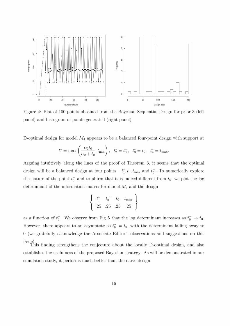
to as Prior 1, Prior 2 and Prior 3 henceforth. The Bayesian sequential algorithm appears to

attain a stable state early, and essentially fluctuates among four points – t∗1, t−0 , t0 and tmax

(where t∗1 is as defined in Theorem 3) – with approximately equal weights. This can be seen

from Figure 4, which plots the selected design points for prior 3 in the sequence they are

generated, including the 10 points of the initial design.

Discussion: From the simulation result described above and shown in Figure 4, the locally

15

0 20 40 60 80 100

050

100

150

200

Number of runs

Des

ign

poin

ts

Design point

Fre

quen

cy

0 50 100 150 200

05

1015

2025

Figure 4: Plot of 100 points obtained from the Bayesian Sequential Design for prior 3 (left

panel) and histogram of points generated (right panel)

D-optimal design for model M4 appears to be a balanced four-point design with support at

t∗1 = max

(α2t0

α2 + t0, tmin

), t∗2 = t−0 , t∗3 = t0, t∗4 = tmax.

Arguing intuitively along the lines of the proof of Theorem 3, it seems that the optimal

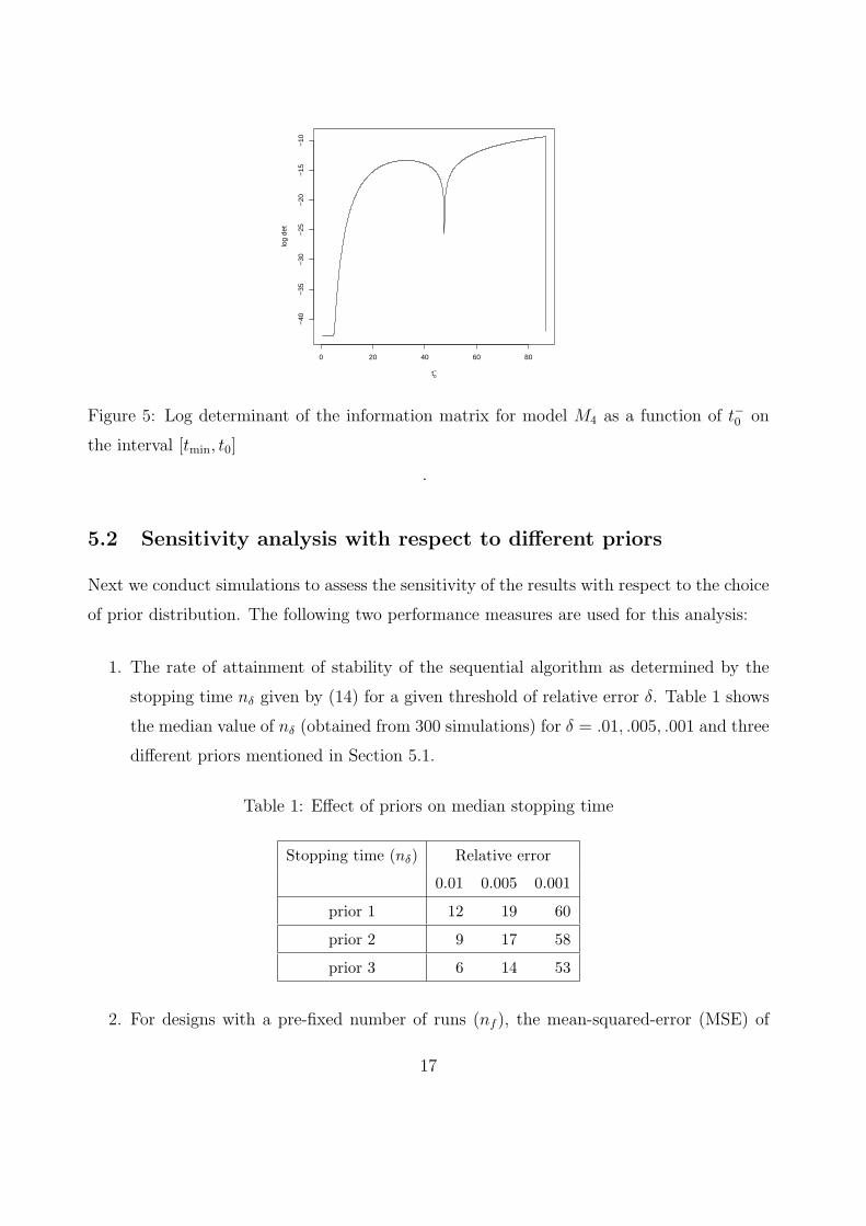
design will be a balanced design at four points – t∗1, t0, tmax and t−0 . To numerically explore

the nature of the point t−0 and to affirm that it is indeed different from t0, we plot the log

determinant of the information matrix for model M4 and the design t∗1 t−0 t0 tmax

.25 .25 .25 .25

as a function of t−0 . We observe from Fig 5 that the log determinant increases as t−0 → t0.

However, there appears to an asymptote as t−0 = t0, with the determinant falling away to

0 (we gratefully acknowledge the Associate Editor’s observations and suggestions on this

issue).This finding strengthens the conjecture about the locally D-optimal design, and also

establishes the usefulness of the proposed Bayesian strategy. As will be demonstrated in our

simulation study, it performs much better than the naive design.

16

0 20 40 60 80

−40

−35

−30

−25

−20

−15

−10

t0−

log

det

Figure 5: Log determinant of the information matrix for model M4 as a function of t−0 on

the interval [tmin, t0]

.

5.2 Sensitivity analysis with respect to different priors

Next we conduct simulations to assess the sensitivity of the results with respect to the choice

of prior distribution. The following two performance measures are used for this analysis:

1. The rate of attainment of stability of the sequential algorithm as determined by the

stopping time nδ given by (14) for a given threshold of relative error δ. Table 1 shows

the median value of nδ (obtained from 300 simulations) for δ = .01, .005, .001 and three

different priors mentioned in Section 5.1.

Table 1: Effect of priors on median stopping time

Stopping time (nδ) Relative error

0.01 0.005 0.001

prior 1 12 19 60

prior 2 9 17 58

prior 3 6 14 53

2. For designs with a pre-fixed number of runs (nf ), the mean-squared-error (MSE) of

17

parameter estimates over repeated simulations. Figure 6 shows the median MSE (ob-

tained from 300 simulations) of estimates of t0 for nf = 10, 20, 30, 40, 50, 60 and three

different priors. The plots of median MSE of estimates of α1, α2, b and σ2 are included

as supplementary material.

10 20 30 40 50 60

02

46

810

12

nf

Med

ian

MS

E fo

r t 0

Prior 1 Prior 2 Prior 3

Figure 6: Effect of priors on the median MSE of estimated t0

From Table 1 and Figure 6, we find that the prior knowledge on t0 improves the stability

and efficiency of the design with respect to estimation of t0. As expected, the MSE of

estimated t0 is smallest when a log-normal prior is used and largest when a uniform prior

is used. The effect of prior distribution on estimation efficiency of t0 is more pronounced

for small number of runs (≤ 20). The stopping time also seems to be somewhat affected by

the choice of prior distribution, although these effects are not as pronounced as the effect of

prior on the MSE of t0.

5.3 Comparison of the Bayesian Sequential Design and Naive De-

sign used by Huang et al.(2011)

Finally, we compare the performance of our design with the naive design strategy adopted

by Huang et al. (2011) to examine whether the proposed strategy really has the potential

to meet the experimenters’ requirements as stated in the introductory section.

We first compare the two designs with respect to their efficiencies of estimation of pa-

rameters for a fixed sample size. Using the same number of design points as in Huang et

18

al. (2011) (19 for no replication, 38 and 57 for one and two replications respectively), the

median root-mean-squared-error (RMSE) of each parameter, obtained from 300 simulations,

is computed for both designs. The results are summarized in Figure 7.

20 30 40 50 60

12

34

5

nf

Med

ian

RM

SE

for

α1

Naive designProposed design

20 30 40 50 60

02

46

810

nf

Med

ian

RM

SE

for

α2

Naive designProposed design

20 30 40 50 60

0.00

070

0.00

075

0.00

080

0.00

085

0.00

090

0.00

095

0.00

100

nf

Med

ian

RM

SE

for

b

Naive designProposed design

20 30 40 50 60

01

23

45

6

nf

Med

ian

RM

SE

for

t 0

Naive designProposed design

20 30 40 50 60

0.01

00.

015

0.02

00.

025

0.03

00.

035

0.04

0

nf

Med

ian

RM

SE

for

σ2

Naive designProposed design

Figure 7: Comparison of the two designs with respect to median RMSE of parameters

Next we conduct simulations to compute the number of runs taken by the proposed

Bayesian sequential strategy to attain the same RMSE of the parameter estimate of the

change point t0 as in 19, 38 and 57-run designs adopted by Huang et al. (2011). The

empirical distribution of the number of such runs obtained from 300 simulations is shown in

Table 2.

From Figure 7 and Table 2, the benefits of the proposed design over the naive strategy

adopted by Huang et al. (2011) are evident. Other than the dispersion parameter σ2 (for

which the results are similar), the RMSEs of the estimated parameters for the proposed

design are much smaller than that of the naive design. Also, the proposed design can help

19

Table 2: Number of runs taken to attain the same efficiency of estimation of the change

point as Huang’s (2011) 19, 38 and 57-run designs

Quantile of number of runs

Number of design points used by Huang(2011)

2.5% 25% median 75% 97.5%

19 2 3 5 7 14

38 3 6 8 11 23

57 3 14 21 29 58

us achieve the same efficiency of the estimate of the change point with far fewer number of

runs (the median number of runs for the proposed design is about one-third of the number

of runs for the naive design). Thus the proposed strategy is expected to be much more cost

effective and efficient compared to the design adopted by Huang et al. (2011) for fitting of

model 4.

6 Concluding remarks

In this paper we have derived a locally D-optimal design for the exponential-linear change

point model that explains the growth of nanostructures. A Bayesian sequential strategy that

converges to the locally D-optimal design corresponding to the true parameter values has

been proposed. Guidelines are proposed for incorporating the experimenters’ perception or

knowledge about the change point into the Bayesian framework through appropriate prior

distributions. The effectiveness of the strategy in comparison to the existing methods has

been demonstrated through a simulation study.

The theoretical framework presented in this paper can be extended to situations with

multivariate inputs. However, establishing closed-form results will be considerably harder as

the dimensions of the geometric problems would increase, based on the number of parameters

in the model. In such cases, one may have to rely on the sequential version, where also

the computational complexity may increase substantially. For such problems, it may be

worthwhile to explore algorithms similar to those proposed by Dror and Steinberg (2008).

20

Although in our problem, prior analysis of data from similar experiments had already

established model M4 as the most appropriate model, there can be situations where the

exact model is unknown. In such situations, it may be possible to use designs for model

discrimination, e.g., the D1 criterion proposed by Dette (1993). Extending such criteria to

the class of non-linear change-point models can be an interesting line of research.

It is worthwhile to note that a batch-sequential approach may sometimes be more effective

than a fully sequential approach, as proposed and studied in our work. It appears that

extending the proposed algorithm to a batch-sequential version will not be very difficult,

and such an extension can be practically useful in many scenarios.

Appendix

Proof of Theorem 2.

Since the volume of the ellipse is given by 1/(AC − B2), to find the minimum volume

ellipse we need to find A,B and C that maximizes AC−B2 subject to Ax21+2Bx1y1+Cy21 = 1

and Ax22 + 2Bx2y2 +Cy22 = 1. Point (x1, y1) is v2(tmax) and (x2, y2) is v2(t

∗1). The objective

function can be written as

S = (AC −B2) + L1(Ax21 + 2Bx1y1 + Cy21 − 1) + L2(Ax

22 + 2Bx2y2 + Cy22 − 1),

where L1 and L2 are Lagrangian multipliers. Differentiating S with respect to A,B and C

and equating them to zero, we obtain

A = −(L1y21 + L2y

22); B = L1x1y1 + L2x2y2; C = −(L1x

21 + L2x

22). (15)

Substituting the values of A,B and C in the two constraints, we obtain

L1 = L2 = −1/(x1y2 − x2y1)2. (16)

The result follows by re-substituting (16) into (15). It is easy to check that the determinant

of the Hessian matrix is -2, which means the objective function is maximized. Substituting

the final expressions of A,B and C into 1/(AC − B2), the volume of the ellipse is obtained

as (x1y2 − x2y1)2.

21

Here we have x1 = v12(tmax) = P ×R and y1 = v22(tmax) = (−α1/t0)P ×Q, where

P = e−α2/t0 , R = 1− α2

t0+

α2tmax

t20, and Q = 2− α2

t0− tmax

t0+

α2tmax

t20.

Since t0 < tmax, it follows that Q < R. Also, we have x2 = e−α2/t∗1 and y2 = (−α1/t∗1)e

−α2/t∗1

where t∗1 ≤ t0.

In order for the ellipsoid to contain v2(t), t ∈ [tmin, tmax], the ellipsoid should be tangent

with v2(t) at t∗1, unless t

∗1 = tmin. Then we have:

(Ax2 +By2) + (Bx2 + Cy2)dy

dx(x2) = 0. (17)

By substituting A,B, x2, y2 and dydx(x2) =

(α1

α2− α1

t∗1

)into (17), we have:(

−α1

t0PQ− PR

(α1

α2

− α1

t∗1

))= 0. (18)

Equation (18) has only one zero point: τ = α2/(1 + α2

t0

QR

). Thus, if tmin < τ , then

t∗1 = τ , otherwise t∗1 = tmin.

It remains to prove that the ellipsoid above contains all points of v2(t), t ∈ [tmin, tmax].

Consider the function:

f(t) = Ax(t)2 + 2Bx(t)y(t) + Cy2(t)− 1, t ∈ [tmin, t0]

The derivative of f(t) is given by:

f ′(t) = −Rα2

t−R− Q

t0α2

t2(

Qt0− R

t

) .

The function f ′(t) only has one zero point, which is τ . It is easy to show that f ′(t) < 0, t > τ

and f ′(t) > 0, t < τ . Thus, f(t) attains its maximum at t∗1 = τ ∨ tmin for t ∈ [tmin, t0].

Consequently, the above ellipsoid contains all points on v2(t), t ∈ [tmin, t0]. The function

v2(t), t0 < t ≤ tmax is a straight line. The ellipsoid contains both v2(t0) and v2(tmax), and

therefore all the points between t0 and tmax.

Proof of Theorem 3.

In this case, we have a ellipsoid in three dimensions, which can be expressed as:

Ax2 +By2 + Cz2 + 2Dxy + 2Exz + 2Fyz = 1. (19)

22

Let the matrix A D E

D B F

E F C

be denoted by S. Then the volume of the ellipsoid is proportional to

√det[S−1] (Sun and

Freund, 2004), which means, to obtain the minimum volume ellipsoid, we need to maximize

det[S] = (AB −D2)C −BE2 + 2DEF − AF 2.

Now we know that the ellipsoid must pass through the point that corresponds to t = tmax.

Denoting this point by(xM , yM , zM), we have from (19)

C =1− Ax2

M −By2M − 2DxMyM − 2ExMzM − 2FyMzMz2M

. (20)

Substituting the above expression of C into det[S], we have

det[S] = (AB −D2)(1− Ax2

M −By2M − 2DxMyMz2M

)− 2E

xM

zM(AB −D2)− 2F

yMzM

(AB −D2)−BE2 + 2DEF − AF 2

= (AB −D2)(1− Ax2

M −By2M − 2DxMyMz2M

)− 2Eβ1 − 2Fβ2 −BE2 + 2DEF − AF 2,

(21)

where β1 = xM

zM(AB −D2), and β2 = yM

zM(AB −D2). Taking the derivative of det[S] with

respect to E,F , we have:

∂ det[S]

∂E= −2EB + 2DF − 2β1,

∂ det[S]

∂F= −2FA+ 2DE − 2β2.

Equating the above partial derivatives to zero, we have: −B D

D −A

E

F

=

β1

β2

. (22)

Substituting E and F from (22) into (21), we have:

det[S] =AB −D2

z2M. (23)

23

Since zM is a constant, the optimization problem in three dimension reduces to maximization

of AB−D2, which is the projection of the ellipsoid on the X −Y plane. Thus, applying the

result of Theorem 1 with tmax = t0, the proof immediately follows. Also, since the projection

of the S on X − Y plane contains v3(t0), then the ellipsoid S will contain points on straight

line v3(t), t ∈ [t0, tmax]. In conclusion, the ellipsoid S contains v3(t), t ∈ [tmin, tmax].

SUPPLEMENTARY MATERIAL

Proof: A detailed proof of Theorem 1. (theorem1proof, pdf file)

R-code: R code implementing the sequential Bayesian algorithm. (zipped file)

Additional figures: Figure on the effect of priors on the median MSE of estimated α1, α2, b

and σ2. (Figure 6.1, pdf file)

ACKNOWLEDGEMENT

We are thankful to the editor, the associate editor and two reviewers whose constructive

suggestions lead to significant improvement in the contents and the presentation of this

paper. The work of Zhu and Dasgupta is supported by the National Science Foundation

under grant number CMMI-1000720. Huang’s work is supported by supported by National

Science Foundation with grant number CMMI-1002580.

REFERENCES

Atkinson, A. C., Donev A. N. and Tobias, R. (2007), Optimum Experimental Designs, With SAS,

Oxford: SAS Oxford University Press.

Atherton, J., Charbonneau, B., Wolfson, D. B., Joseph, L., Zhou, X., and Vandal, A. C. (2009).

“Bayesian Optimal Design for Changepoint Problems,” Canadian Journal of Statistics, 37,

495-513.

Biedermann, S., Dette, H., and Woods, D. C. (2011), “Optimal Designs for additive partially

nonlinear models,” Biometerika, 98, 449-458.

24

Box, G. E. P. and Hunter, W. G. (1965), “Sequential Design of Experiments for Nonlinear Models,”

in Proceedings of the IBM Scientific Computing Symposium on Statistics, October 21-23,

1963, pp. 113-137.

Chaloner, K. and Larntz, K. (1989), “Optimal Bayesian Design Applied to Logistic Regression

Experiments,” Journal of Statistical Planning and Inference, 21, 191208.

Chaloner, K. and Verdinelli, I. (1995), “Bayesian Experimental Design: A Review,” Statistical

Science, 10, 273304.

Chaudhuri, P. and Mykland, P. A. (1993), “Nonlinear Experiments: Optimal design and Inference

Based on Likelihood,” Journal of the American Statistical Association, 88, 538-546.

Chernoff, H. (1953), “Locally Optimal Designs for Estimating Parameters,” Annals of Mathemat-

ical Statistics, 30, 586-602.

Chernoff, H. (1975), “Approaches in Sequential Design of Experiments,” in A Survey of Statistical

design and Linear Models, ed. J. N. Srivastava, New York: North-Holland, pp. 67-90.

Dasgupta, T., Ma, C., Joseph, R., Wang, Z. L. and Wu, C. F. J. (2008), “Statistical Modeling

and Analysis for Robust Synthesis of Nanostructures,” Journal of the American Statistical

Association, 103 (482), 594-603.

Dette, H. (1993), “On a mixture of the D− and D1−optimality Criterion in Polynomial Regres-

sion,” Journal of Statistical Planning and Inference, 35, 233-249.

Dror, H.A. and Steinberg, D. M. (2008), “Sequential Experimental Designs for generalized Linear

Models,” Journal of the American Statistical Association, 103, 288-298.

Dubrovskii, V. G., Sibirev, N. V., Cirlin, G. E., Harmand, J. C., Ustinov, V. M. (2006). “Theo-

retical Analysis of the Vapor-Liquid-Solid Mechanism of Nanowire Growth During Molecular

Beam Epitaxy,” Physical review, E Vol. 73, 021603.

Federov, V. V. (1972), Theory of Optimal Experiments, New York: Academic Press.

Ford, I. and Silvey, S. D. (1980), “A Sequentially Constructed Design for Estimating a Nonlinear

Parametric Function,” Biometrika 67, 381-388.

Ford, I., Torsney, B., and Wu, C. F. J. (1992), “The Use of a Canonical Form in the Construction of

Locally Optimal Designs for Non-Linear problems,” Journal of the Royal Statistical Society,

Ser. B, 54, 569-583.

25

Haines, L. M. (1993), “Optimal Designs for Nonlinear regression Models,” Communications in

Statistics, Part A - Theory and Methods, 22, 1613-1627.

Hohmann, G. and Jung, W. (1975), “On Sequential and Nonsequential D-Optimal Experiment

Design,” Biometrisch Zeitschrift, 17, 329-226.

Huang, Q. (2011), “Physics-Driven Bayesian Hierarchical Modeling of Nanowire Growth Process

At Each Scale,” IIE Transactions, 43, 1-11.

Huang, Q., Wang, L., Dasgupta, T., Zhu, L., Sekhar, P. K., Bhansali, S., and An, Y. (2011),

“Statistical Weight Kinetics Modeling and Estimation for Silica Nanowire Growth Catalyzed

by Pd Thin Film,” IEEE Transactions on Automation Sciences and Engineering, 8, 303-310.

Kikkawa, J., Ohno, Y., Takeda, S. (2005), “Growth Rate of Silicon Nanowires,” Applied Physics

Letters, 4, 123109.

Liu. J. (2002), “Monte Carlo Strategies in Scientific Computing,” New York: Springer.

Lu, J.C., Jeng, S. L. and Wang, K. (2009), “A Review of Statistical Methods for Quality Improve-

ment and Control in Nanotechnology,” Journal of Quality Technology, 41, 148-164.

Mukhopadhyay, S. and Haines, L. M. (1995), “Bayesian D-optimal Designs for the Exponential

Growth Model ,” Journal of Statistical Planning and Inference, 44, 385-397.

Roy, A., Ghosal, S. and Rosenberger, W. F. (2009), “Convergence properties of sequential Bayesian

D-optimal designs,” Journal of Statistical Planning and Inference, 139, 425-440.

Ruth, V., and Hirth, J. P. (1964), “Kinetics of Diffusion-Controlled Whisker Growth,” Journal of

Chemical Physics, 41, 3139-3149.

Sibson, R. (1972), “Contribution to Discussion of papers by H. P. Wynn and P. J. Laycock”,

Journal of the Royal Statistical Society, Ser. B, 34, 181-183.

Silvey, S. D. (1972), “Contribution to Discussion of papers by H. P. Wynn and P. J. Laycock”,

Journal of the Royal Statistical Society, Ser. B, 34, 174-175.

Silvey, S. D. (1980), Optimal Design, London: Chapman and Hall.

Silvey, S. D. and Titterington, D. M. (1973), “A Geometric Approach to Optimal Design Theory”,

Biometrika, 60, 21-32.

26

Sun, P. and Freund, R. M. (2004), “Computation of Minimum-Volume Covering Ellipsoids,”

Operations Research, 52, 690-706.

Titterington, D. M. (1975), “Optimal Design: Some Geometrical Aspects of D-Optimality”,

Biometrika, 62, 313-320.

Vandenberghe, L., Boyd, S. and Wu, S. (1998), “Determinant Maximization with Linear Matrix

Inequality Constraints”, Siam Journal of Matrix Analysis and Applications, 19, 499-533.

27