a critical assessment of the truly meshless local petrov-galerkin (mlpg),
TRANSCRIPT

8/6/2019 A Critical Assessment of the Truly Meshless Local Petrov-Galerkin (MLPG),
http://slidepdf.com/reader/full/a-critical-assessment-of-the-truly-meshless-local-petrov-galerkin-mlpg 1/25
A critical assessment of the truly Meshless Local Petrov-Galerkin (Mand Local Boundary Integral Equation (LBIE) methods
S. N. Atluri, H.-G. Kim, J. Y. Cho
Abstract The essential features of the Meshless LocalPetrov-Galerkin (MLPG) method, and of the Local Boun-dary Integral Equation (LBIE) method, are critically ex-amined from the points of view of a non-elementinterpolation of the ®eld variables, and of the meshlessnumerical integration of the weak form to generate thestiffness matrix. As truly meshless methods, the MLPG andthe LBIE methods hold a great promise in computationalmechanics, because these methods do not require a mesh,either to construct the shape functions, or to integrate thePetrov-Galerkin weak form. The characteristics of variousmeshless interpolations, such as the moving least square,Shepard function, and partition of unity, as candidates fortrial and test functions are investigated, and the advan-tages and disadvantages are pointed out. Emphasis isplaced on the characteristics of the global forms of thenodal trial and test functions, which are non-zero only over local sub-domains X J
tr and X I te , respectively. These
nodal trial and test functions are centered at the nodes J and I (which are the centers of the domains X J
tr and X I te),
respectively, and, in general, vanish at the boundaries o X J tr
and o X I te of X J
tr and X I te , respectively. The local domains
X J tr and X
I te can be of arbitrary shapes, such as spheres,
rectangular parallelopipeds, and ellipsoids, in 3-Dimen-sional geometries. The sizes of X J
tr and X I te can be arbi-
trary, different from each other, and different for each J ,and I , in general. It is shown that the LBIE is but a specialform of the MLPG, if the nodal test functions are speci®-cally chosen so as to be the modi®ed fundamental solu-tions to the differential equations in X I
te , and to vanish atthe boundary o X I
te . The dif®culty in the numerical inte-gration of the weak form, to generate the stiffness matrix,is discussed, and a new integration method is proposed. Inthis new method, the I th row in the stiffness matrix isgenerated by integrating over the ®xed sub-domain X I
te(which is the support for the test function centered at nodeI ); or, alternatively the entry KIJ in the global stiffnessmatrix is generated by integrating over the intersections of the sub-domain X J
tr (which is the sub-domain, with node J
as its center, and over which the trial function is non-zero), with X I
te (which is the sub-domain centered at nodeI over which the test function is non-zero). The generality of the MLPG method is emphasized, and it is pointed thatthe MLPG can also be the basis of a Galerkin method thatleads to a symmetric stiffness matrix. This paper alsopoints out a new but elementary method, to satisfy theessential boundary conditions exactly, in the MLPGmethod, while using meshless interpolations of the MLStype. This paper presents a critical appraisal of the basicframeworks of the truly meshless MLPG/LBIE methods,and the numerical examples show that the MLPG approachgives good results. It now apears that the MLPG methodmay replace the well-known Galerkin ®nite elementmethod (GFEM) as a general tool for numerical modeling,in the not too distant a future.
1IntroductionThe development of approximate methods for the nu-merical solutions of partial differential equations has at-tracted the attention of engineers, physicists andmathematicians for a long time. In recent years, meshlessmethods, as alternative numerical approaches to eliminatethe known drawbacks in the well-known ®nite elementmethod, have been developed to solve problems, withoutthe human-labor intensive process of constructing geo-metric meshes in a domain. Meshless methods may alsoalleviate some other problems associated with the ®niteelement method, such as locking, element distortion, re-meshing during large deformations, and others. Moreover,nodes can be easily added or removed, as the deformationprogresses, and more accurate solutions for the solutionvariables, as well as their spatial gradients, can, in general,be obtained using meshless methods. Several meshlessmethods (Smooth Particle Hydrodynamics (SPH) by Gin-
gold and Monaghan 1977; Element Free Galerkin (EFG) by Belytschko et al. 1994; Reproducing Kernel ParticleMethod (RKPM) by Liu et al. 1995; the Partition of Unity Finite Element Method (PUFEM) by Babuska and Melenk1997; hp-cloud method by Duarte and Oden 1996; NaturalElement Method (NEM) by Sukumar et al. 1998) have beendeveloped to solve boundary value problems. The majordifferences in these meshless methods come only from theinterpolation techniques used. In particular, the abovecited meshless methods are ``meshless'' only from thepoint of view of the interpolation of the ®eld variables, ascompared to the usual ®nite element method. Althoughspecial approaches to interpolate a function, using ran-domly scattered data have been investigated for a long
Computational Mechanics 24 (1999) 348±372 Ó Springer-Verlag 1999
348
Received 15 January 1999
S.N. Atluri (8 ), H.-G. Kim, J.Y. ChoCenter for Aerospace Research & Education, 7704 Boelter Hall,University of California, Los Angeles, CA 90095-1600, USA
This work was supported by the of®ce of Naval Research, withDr. Y.D.S. Rajapakse as the cognizant program of®cial, and by NASA Langley Research Center, with Dr. I.S. Raju as thecognizant program of®cial.

8/6/2019 A Critical Assessment of the Truly Meshless Local Petrov-Galerkin (MLPG),
http://slidepdf.com/reader/full/a-critical-assessment-of-the-truly-meshless-local-petrov-galerkin-mlpg 2/25
time, a proper meshless interpolation technique is stillneeded to make meshless methods stable and robust, withsimple computations. Popular interpolation schemes usedin the meshless methods are the Moving Least Square(MLS) proposed by Lancaster and Salkauskas (1981), andthe Partition of Unity (PU) proposed by Babuska andMelenk (1997). In this paper, these meshless interpolationschemes, including the Shepard functions, are studiedfrom the points of view of the intrinsic characteristics of nodal shape functions (i.e. the non-zero functions overeach X I
tr ) generated by these schemes, and of the dif®-culties in the numerical integration of the weak formsassociated with these nodal shape functions. We assess thereasons also why it is not adequate to integrate the weakform, using only small numbers of Gaussian-quadratureintegration points in the domain of integration. Mostmeshless methods in prior literature have used back-ground cells, to integrate a global Galerkin weak form.These kinds of background cells for integration of theglobal weak form do not make for a truly meshless
method. On the other hand, the Meshless Local Petrov-Galerkin (MLPG) method by Atluri and Zhu (1998a, b,1999) proposed a new integration method in a local do-main, based on a Local Symmetric Weak Form (LSWF).Consequently, the MLPG method introduced a new con-cept in the ®eld of meshless methods. It should be em-phasized that the MLPG method is based on a local weakformulation; and any non-element interpolation schemesuch as the MLS, the PU, or Shepard functions can be usedas trial and test functions. Integrating the weak form in alocal domain may be a natural choice, considering that thelocal sub-domains in the MLPG method can be chosen tobe circles, ellipses, or rectangles in 2-D; and spheres,rectangular parallelopipeds, and ellipsoids in 3-D. There-fore, the MLPG method is a truly meshless method, and allother meshless methods can be derived from it, as specialcases, if the trial and test functions and the integrationmethods are selected appropriately. Furthermore, theMLPG method with different spaces for test and trialfunctions has a generality and an advantage over othermeshless methods, especially for ¯uid mechanics prob-lems. In addition, the MLPG method does not require an``assembly'' process in the course of forming the ``stiffnessmatrix''. Another promising meshless method, for solvingboundary-value problems, is the Local Boundary IntegralEquation (LBIE) method (Zhu et al. 1998a, b). Thismethod requires no domain and/or boundary ``elements''
to implement the formulation. However, singular integralsappear in the local boundary integral equation, to whichspecial attention should be paid. It is shown in the presentpaper that the LBIE approach can be treated simply as aspecial case of the MLPG approach.
In summary, the MLPG is a truly meshless method thatinvolves not only non-element interpolation (such as MLS,PU, or Shepard function), but also non-element integra-tion (i.e. all integrations are always performed over regu-larly shaped sub-domains such as spheres, parallelopipeds,and ellipsoids, in 3-D, or their intersections). In general, inMLPG, the nodal shape functions for trial and test func-tions are non-zero only over regular-shaped (such asspheres, parallelopipeds, and ellipsoids) sub-domains,
with the concerned node being the center of the sub-do-main. In the following, we consider X J
tr to be the sub-domain, with the node J as its center, and over which thenodal-trial-shape function is non-zero; and X I
te to be thesub-domain, with the node I as its center, and over whichthe nodal-test-shape function is non-zero. These nodaltrial and test functions can, in general, be different (i.e. thenodal trial function may correspond to any one of MLS,PU, or Shepard interpolations; and the nodal test functionmay be totally different, and corresponding to any one of MLS, PU, Shepard, or a special form of the fundamentalsolution to the differential equation in X I
te). Furthermore,the sizes of the sub-domains over which the nodal trial andtest functions are, respectively, non-zero, i.e. the sizes of X J
tr and X I te may be different. In these general situations,
the MLPG method leads to non-symmetric ``stiffnessequations''. On the other hand, if the nodal trial and testfunctions both correspond to the same non-element-in-terpolation scheme, and if X J
tr and X I te are of the same size
for each I and J , the MLPG method leads to symmetric
stiffness equations. These concepts are clearly illustratedin this paper.In the present work, the various features of the MLPG
approach are illustrated through solving elasto-staticproblems. Essential boundary conditions are enforcedwhile using the meshless approximations, either approxi-mately by using a penalty formulation as in (Zhu et al.1998), or exactly by using a new but elementary methoddeveloped in this paper. It is much easier to employ thepenalty method than using the Lagrange multiplier tech-nique, because additional equations and non-positivede®nite matrices can be avoided. Various non-elementinterpolation schemes, such as MLS, PU and Shepard, arecritically reviewed with an emphasis on the characteristicsof the resulting nodal shape functions. Special attention ispaid to the derivatives of nodal shape functions, in con-nection with the numerical integration of the attendantPetrov-Galerkin weak forms. The interpolation-error-es-timate for meshless interpolations, as a general concept, isstudied, through a numerical approach. Fundamentally,the bound for the interpolation error in meshless inter-polations affects the numerical results in the MLPGmethod, even if the weak form is evaluated exactly. Un-fortunately, however, the nodal shape functions frommeshless interpolations, such as MLS, Shepard, PU, or hp-clouds, are highly complex in nature, which makes anaccurate numerical integration of the weak form highly
dif®cult. We present here new integration methods, forintegrating the local symmetric weak form of MLPG overeach sub-domain X I
te (circle, rectangles, and ellipses in 2-D; and spheres, parallelopipeds, and ellipsoids in 3-D) orover intersections of such sub-domains ( X I
te and X J tr ) to
compute the global stiffness matrix directly, without theusual ``assembly'' as in the Galerkin ®nite element method.To perform the integrations for local sub-domains X I
te thatintersect with global boundary C , a technique to map thedomain of intersection into a unit-circle (in 2-D) is used.We show some numerical results for the rates of conver-gence in problems of a cantilever beam, and of a plate witha hole. Moreover, we show that elliptical shaped sub-do-mains X I
teand X J
tr, for problems with different nodal
3

8/6/2019 A Critical Assessment of the Truly Meshless Local Petrov-Galerkin (MLPG),
http://slidepdf.com/reader/full/a-critical-assessment-of-the-truly-meshless-local-petrov-galerkin-mlpg 3/25
spacing along the x- and y-directions, respectively, givebetter solutions than circular shaped sub-domains. Thenumerical examples in Sect. 6 illustrate the performance of the MLPG method, in two-dimensional elasticity prob-lems. We show that the basic framework of the MLPGmethod is very versatile indeed, and holds a great promiseto replace the ®nite element method, as a method of choice, someday in the not-too distant future.
2The Global Weak Form; Galerkin Finite Element Method;Global Forms of nodal trial & test functions;and the symmetric stiffnessConsider the problem of two-dimensional linear elasticity in a global domain X , bounded by C , where the equationsof equilibrium are given by
r ijY j bi 0 in X 1
where r ij is the stress tensor, bi are the body forces, Y j
denoteso
ao
x j, and a summation over a repeated index isimplied. The boundary conditions are assumed to be:
ui "ui at C u Y 2ar ijn j
"t i at C t X 2b
Assuming linear-elastic behavior, one has:
r ij Eijkl u kYl 3
where
u kYl 12 ukYl ul YkÀ ÁX 4
The Galerkin Finite Element Method (GFEM) is based onthe Global Symmetric Weak Form (GSWF):
XEijkl v iY j u kYl À bivi ÃdX À C t
"t ivi dC 0 5
for all trial functions ui that are continuous in each ele-ment, as well as at the interelement boundaries, and satisfy the essential b.c. at C u a priori; and for all test functions vithat are continuous in each element as well as at the inter-element boundaries, and satisfy the condition vi 0 at C u ,a priori. Under these conditions, Eq. (5) may be written as:
m X m& Eijkl v iY j u kYl À bivi ÃdX À C tm
"t ivi dC ' 0
6
where the sum extends over all ®nite elements X m , andtheir boundaries C tm . In the usual ®nite element method,one assumes the trial and test functions over each element,as:
ui x a
/ a x uai Y 7
vi x a
/ a x vai 8
where the summation in (7) and (8) extends over all theelement nodes a , and where the nodal values of the trialand test functions are va
i and uai . Thus / a x in (7) and (8)
may be called the ``element-nodal shape functions'', and
each has a value of unity of the node a . From (6)±(8) it isimmediately evident that the usual Galerkin Finite ElementMethod (GFEM) introduces elements and element meshes,not only for interpolation purposes (7) and (8), but alsofor integration of weak form (6) purposes. If the elementthat is used, say in a two dimension, is a triangle, in theelasticity problem (6), the element-nodal shape functionsfor trial as well as test functions are linear.
On the other hand, the ``global-nodal-shape functions'',for the elasticity problem in 2-D, are clearly functions suchthat they have a value of unity at the node in question, andgo to zero at all the immediately surrounding nodes, aswell as at the boundary of the star X J
tr surrounding thenode J in question, as shown in Fig. 1. The global weakform (6) may be alternatively written, in terms of theglobal-nodal-shape functions, as:
I Y J X I te
Eijkl / I Y jv
I i /
J Yl u
J k À bi/ I vI
i dX À C I t
"t i/ I vI i dC 0
9
where / J are the global-nodal-trial-shape functions cen-tered at node J (and have values of unity at node J ) and arenon-zero only over X J
tr , and / I are the global-nodal-test-shape functions centered at node I and are non-zero only
a
b
Nodal test function
Nodal trial function
I
J
Fig. 1. a Test function centered at node I , non-zero in X I te and
vanishes at o X I te ; trial function centered at node J , non-zero in X J
trand vanishes at o X J
tr . b The intersection of test function in X I te ,
and the trial function in X J
tr, contributes to the stiffness term KIJ
350
8/6/2019 A Critical Assessment of the Truly Meshless Local Petrov-Galerkin (MLPG),
http://slidepdf.com/reader/full/a-critical-assessment-of-the-truly-meshless-local-petrov-galerkin-mlpg 4/25
over X I te , as shown in Fig. 1. Further, u J
k are the nodalvalues of the trial function uk, and vI
i are the nodal valuesof the test function vi.
It is immediately clear from Eq. (9) and Fig. 1, that theentry KIJ in the global stiffness matrix is such that:
KIJ 0 10
unless the node J is an immediate neighbor of node I , i.e.node J is a vertex of the star X I
te surrounding the node I .This is the reason for the banded-symmetric nature of KIJ in GFEM. It is also important to note, to compare andcontrast the GFEM with the MLPG, later in this paper, thatthe non-zero KIJ is the result of integrating an integrandwhich is non-zero only over the intersection of the do-mains X J
tr and X I te surrounding nodes J and I , respectively,
as shown in Fig. 1. In reality however, in GFEM, the weakform is integrated over all contiguous ®nite elements, andthe respective `nodal contributions' are assembled, to formthe global stiffness matrix.
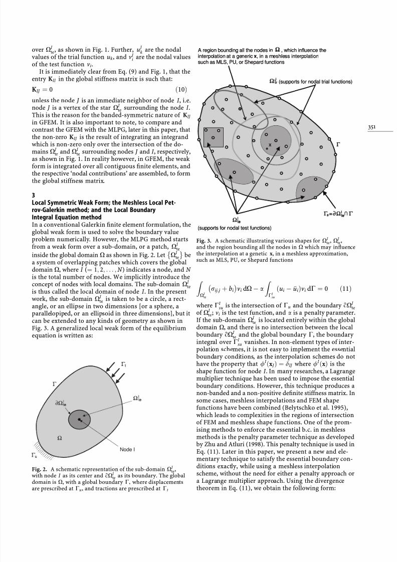
3Local Symmetric Weak Form; the Meshless Local Pet-rov-Galerkin method; and the Local BoundaryIntegral Equation methodIn a conventional Galerkin ®nite element formulation, theglobal weak form is used to solve the boundary valueproblem numerically. However, the MLPG method startsfrom a weak form over a sub-domain, or a patch, X I
teinside the global domain X as shown in Fig. 2. Let X I
teÈ Ébea system of overlapping patches which covers the globaldomain X , where I ( 1Y2YF F FYN ) indicates a node, and N is the total number of nodes. We implicitly introduce theconcept of nodes with local domains. The sub-domain X I
teis thus called the local domain of node I . In the presentwork, the sub-domain X I
te is taken to be a circle, a rect-angle, or an ellipse in two dimensions [or a sphere, aparallelopiped, or an ellipsoid in three dimensions], but itcan be extended to any kinds of geometry as shown inFig. 3. A generalized local weak form of the equilibriumequation is written as:
X I te
r ijY j bi
À Ávi dX À a C I su
ui À "u i vi dC 0 11
where C I su is the intersection of C u and the boundary o X I
teof X I
te ; vi is the test function, and a is a penalty parameter.If the sub-domain X I
te is located entirely within the globaldomain X , and there is no intersection between the localboundary o X I
te and the global boundary C , the boundary integral over C I
su vanishes. In non-element types of inter-polation schemes, it is not easy to implement the essentialboundary conditions, as the interpolation schemes do nothave the property that / I x J dIJ where / I x is theshape function for node I . In many researches, a Lagrangemultiplier technique has been used to impose the essentialboundary conditions. However, this technique produces a
non-banded and a non-positive de®nite stiffness matrix. Insome cases, meshless interpolations and FEM shapefunctions have been combined (Belytschko et al. 1995),which leads to complexities in the regions of intersectionof FEM and meshless shape functions. One of the prom-ising methods to enforce the essential b.c. in meshlessmethods is the penalty parameter technique as developedby Zhu and Atluri (1998). This penalty technique is used inEq. (11). Later in this paper, we present a new and ele-mentary technique to satisfy the essential boundary con-ditions exactly, while using a meshless interpolationscheme, without the need for either a penalty approach ora Lagrange multiplier approach. Using the divergencetheorem in Eq. (11), we obtain the following form:
Node I
Fig. 2. A schematic representation of the sub-domain X I te,
with node I as its center and o X I te as its boundary. The global
domain is X , with a global boundary C , where displacementsare prescribed at C u , and tractions are prescribed at C t
x
(supports for nodal trial functions)
(supports for nodal test functions)
A region bounding all the nodes in , which influence theinterpolation at a generic , in a meshless interpolationsuch as MLS, PU, or Shepard functions
x
x
(supports for nodal trial functions)
(supports for nodal test functions)
A region bounding all the nodes in , which influence theinterpolation at a generic , in a meshless interpolationsuch as MLS, PU, or Shepard functions
x
Fig. 3. A schematic illustrating various shapes for X I te , X J
tr ,and the region bounding all the nodes in X which may in¯uencethe interpolation at a genetic x , in a meshless approximation,such as MLS, PU, or Shepard functions
3

8/6/2019 A Critical Assessment of the Truly Meshless Local Petrov-Galerkin (MLPG),
http://slidepdf.com/reader/full/a-critical-assessment-of-the-truly-meshless-local-petrov-galerkin-mlpg 5/25
o X I te
r ijn jvi dC À X I te
r ijviY j À biviÀ ÁdX
À a C I su
ui À "u i vi dC 0 12
where n j is the outward unit normal to the boundary o X I teX
In the following development, the Petrov-Galerkinmethod is used. Unlike in the conventional Galerkinmethod in which the trial and test functions are chosenfrom the same space, the Petrov-Galerkin method uses thetrial functions and test functions from different spaces. Inparticular, the test functions need not vanish on theboundary where the essential boundary conditions arespeci®ed. Also, in order to simplify the above Eq. (12), wedeliberately select the test functions vi such that they vanishover o X I
te , except when o X I te intersects with the global
boundary C . This can be easily accomplished in the MLPGmethod by using the nodal-test-shape function whose valueat the local boundary o X I
te is zero, as long as o X I te does not
intersect with C . The schematic descriptions for the trialand test functions in the MLPG are shown in Fig. 4. Usingthese test functions in Eq. (12), we obtain the followingLocal Symmetric Weak Form (LSWF) in linear elasticity:
X I te
r ijviY j dX a C I su
uivi dC À C I su
t ivi dC
C I st
"t ivi dC a C I su
"uivi dC X I te
bivi dX 13
where t i r ijn j, and C I st is the intersection of C t and the
boundary o X I te of X I
te . The MLPG method, based on thelocal formulation (11) makes the basic concepts for inte-grating the local weak form (13), and the generation of theglobal stiffness matrix to be quite different from the usedGalerkin FEM. The MLPG formulation enables us to usedifferent interpolations for trial and test functions. Fur-thermore, the sizes and shapes of the sub-domains whichare as supports (i.e. the sub-domains X J
tr and X I te over
which the trial and test functions are, respectively, non-
zero) of trial and test functions do not need to be of thesame size or shape in the MLPG formulation. Therefore,the MLPG method can include all other meshless methodsas special cases. The MLPG method is schematically illus-trated in Fig. 5. X I
te is the sub-domain (in this illustration,a circle) over which the test function, centered at the nodeI in non-zero. X J
tris the sub-domain (in this illustration,
also a circle, but with a radius which is different from thatof X I
te) over which the trial function, centered at node J , isnon-zero. Note, however, that the value the trial functionat each point x inside X I
te is in¯uenced by a set of (perhaps®ctitious, as in MLS) values of the function at an arbitrary number (as determined, for instance, by the radius of theweight function in an MLS interpolation) of nodes in thevicinity of each x . Thus, Eq. (13) leads, for each X I
te , to theI th equation in the system stiffness matrix, involving allthe J nodes, whose sub-domains X J
tr intersect with X I te ,
such that the integrand in Eq. (13) is non-zero. It is seenthat if the radius of X J
tr and X I te are the same for each J and
I , and further, if the trial and test functions centered at
node J and I are the same for each J and I , the globalstiffness matrix will be symmetric; otherwise not.The contrasting features of the MLPG method and the
usual Galerkin Finite Element Method can be understoodby comparing Figs. 1, 6, and 7. In Fig. 1a, in GFEM, there isa mesh; and in the elasticity problem, the test function inX I
te is a pyramid, and each equation in GFEM corre-sponding to each I arises out of the non-zero value of theweak form, in X I
te , as this pyramid test function `intersects'with a piecewise linear trial function (see also Fig. 7a). It iswell known that in the GFEM, that this equation for each I implies a weak form of not only the differential equation of equilibrium in X I
te , but also the weak forms of the tractionreciprocity conditions at all the inter-element boundariesmeeting at the node I (see Fig. 7a). On the other hand, inFigs. 4 and 7b, in MLPG, there is no mesh; the nodal testfunction in a non-element interpolation, such as MLS, is a`smooth tent', and each equation in MLPG correspondingto each node I arises out of the non-zero value of the weakform, in X I
te , as this `smooth tent' intersects with a
I te Test function in Ω
J tr Trial functions in Ω
Fig. 4. Intersections of trial functions inX J
tr J 1Y2YF F FYn with the test functionX I
te . Illustrations is for circular shapes forboth X J
tr and X I te , but with different radii.
How many X J tr intersect with the speci®c
X I te depends on the nodal spacing, and
the radii of X J
trand X I
te
352

8/6/2019 A Critical Assessment of the Truly Meshless Local Petrov-Galerkin (MLPG),
http://slidepdf.com/reader/full/a-critical-assessment-of-the-truly-meshless-local-petrov-galerkin-mlpg 6/25
Fig. 5. Schematics of the MLPG and theLBIE methods
)( xJ φ
J tr Ω
J
I
I te Ω
)( xI ψ
MLPG :
LL
Shepard
PU
MLS
Trial
LL
Shepard
PU
MLS
Test
LL
Ellipse
Rectangle
Circle
Shapes
: Weak form
∫ ∫ ∫ Ω Γ Γ Γ −Γ +ΩI
te I su
I su
d v t d v u d v i i i i j i ij ασ , ∫ ∫ ∫ Γ Γ ΩΩ+Γ +Γ = I
st I su
I te
d v b d v u d v t i i i i i i α
LBIE :
LLShepard
PU
MLS
TrialSolution
FundamentalTest
LLEllipse
Rectangle
Circle
Shapes
: Weak form
∫ ∫ ∫ ∫ Γ Γ ΩΩ∂Γ +Γ +Ω+Γ −= I
st I su
I te
I te
d v t d v t d v b d u t u i i i i i i l l I l ****)(x
Fig. 6. The region of intersection of X I te
and X J tr , wherein the local symmetric
weak form, involving the derivatives of wI x and / J x is non-zero. Only thisnon-zero integrand contributes the entry of KIJ in the global stiffness matrix
3

8/6/2019 A Critical Assessment of the Truly Meshless Local Petrov-Galerkin (MLPG),
http://slidepdf.com/reader/full/a-critical-assessment-of-the-truly-meshless-local-petrov-galerkin-mlpg 7/25
`smooth' trial function. Thus, in MLPG, in general, eachequation for each node I is more likely to imply the weakform of only the differential equation in X I
te . Thus, theperformance of the MLPG method may be expected to besuperior to that of the GFEM.
We again emphasize that, in Eq. (13), test functions inX I
te vanish at o X I te as long as o X I
te does not intersect with C ;
and insideX I
te they can be derived from anyone of: MLS,PU, Shepard or other meshless interpolation strategies.Likewise, the trial function in each X J
tr vanishes at o X J tr ; and
inside X J tr , they can be derived from any one of: MLS, PS, or
Shepard or any other meshless interpolation strategies.We now consider a further novelty when the test
function in X I te not only vanishes at o X I
te as long as o X I te
does not intersect with C ; but inside X I te, it is also a fun-
damental solution to the differential equation inside X I te
(in the elasticity problem, it is a singular solution corre-sponding to a point load at the node I ). In this case also,we consider that the trial functions, however, in each X J
trvanish at o X J
tr as long as o X I te does not intersect with C ;
and inside X J
tr, they can be derived from anyone of: MLS,
PS, or Shepard function or any other meshless interpol-ation strategies. For this purpose, we note that: X I
te
r ijviY j dX X I te
ukYl Eijkl viY j dX
o X I te
Eijkl viY j
À Ánl uk dC
À X I te
Eijkl viY jÀ ÁYl uk dX X 14
Let vÃi be the fundamental solution to the differential
equation:
Eijkl vÃiY j Yk
dl x À x I 0 15
where dl x À x I is a point load along the cartesian di-rection x l at the node I , with the location x I . Further, it isimportant to note that vÃ
i is chosen, such that:
vÃi 0 at o X I
te X 16
Let
t Ãl Eijkl vÃiY j nk at o X I
te X 17
Using Eqs. (15)±(17) in Eq. (14), one obtains: X I te
r ijvÃiY j dX o X I
te
t Ãl u l dC u l x I X 18
Substituting Eq. (18) in Eq. (13), one obtains:
ul x I À o X I te
t Ãl x Yx I ul x dC X I te
bi x vÃi x Yx I dX
a C I su
"u i x À ui x vÃi x Yx I dC
C I st
"t i x vÃi x Yx I dC C I
su
t i x vÃi x Yx I dC X
19
If o X I te intersects with the overall boundary C of the global
domain X , the two last terms in Eq. (19) may be retained.However, since Eq. (19) is valid everywhere in X I
te , and ono X I
te , including at the intersection of o X I te with C su, the
essential b.c. can be directly imposed on ul x I . Thus, thepenalty term, i.e. the 3rd term on the right-hand-side of Eq. (19) is super¯uous, and may be dropped. Thus, theunsymmetric weak form governing the LBIE based mesh-less method can be written as:
ul x I À o X I te
t Ãl x Yx I ul x dC X I te
bi x vÃi x Yx I dX
C I st
"t i x vÃi x Yx I dC C I
su
t i x vÃi x Yx I dC X
20
The kernel t Ãl x Yx I is singular; and regularization proce-dures can be employed, as usual (see Sladek et al. 1999).
The modus operandi of the LBIE method can be un-derstood from Figs. 4±6. Equation (20) relates the values of displacements u
l at the node I , to the values of u
l on o X I
te
Trial function
Trial function
Physical domain
Physical domain
Test function
I
I
a
b
Test function
Fig. 7a,b. Comparison of the basic concepts ( a) in the General®nite element method, and ( b) in the MLPG method
354

8/6/2019 A Critical Assessment of the Truly Meshless Local Petrov-Galerkin (MLPG),
http://slidepdf.com/reader/full/a-critical-assessment-of-the-truly-meshless-local-petrov-galerkin-mlpg 8/25

8/6/2019 A Critical Assessment of the Truly Meshless Local Petrov-Galerkin (MLPG),
http://slidepdf.com/reader/full/a-critical-assessment-of-the-truly-meshless-local-petrov-galerkin-mlpg 9/25
where B ~x is a sphere centered at ~x , pT x p1 x Y p2 x YF F FY pm x is a complete monomial basis of order m;and a ~x is a vector containing the coef®cientsa j ~x Yj 1Y2YF F FYm which are functions of the space
coordinates x xY yYz T
. The commonly used bases in 2-D problems are the linear basis:
pT x 1YxY y 26
or the quadratic basis:
pT x 1YxY yYx2YxyY y2
 ÃX 27
The coef®cient vector a ~x is determined by minimizing aweighted discrete L2-norm with respect to nodal points,de®ned as:
Y ~x N
I 1wI ~x pT x I a ~x À uI
 Ã
2
P Áa ~x À u TÁW ~x Á P Áa ~x À u 28
where wI ~x is a weight function de®ned in a sub-domainX I
tr , with the node I as its center; and with wI ~x b 0 for all~x in the support of wI ~x and wI ~x 0 at the boundary of X I
tr , x I denotes the value of x at node I , and the matrices Pand W are de®ned as:
P
pT x 1pT x 2
F F F
pT x N
PTTRQUUSN Âm
Y 29
W ~x w1 ~x F F F 0
F F F F F F F F F0 F F F wN ~x PR QSN ÂN
30
and
uT u1Yu2YF F FYuN
 ÃX 31
Here it should be noted that uI YI 1Y2YF F FYN are the®ctitious nodal values. In fact, only those neighboringnodes J , whose sub-domains X J
tr intersect with the sub-domain X I
tr of node I , have an in¯uence in constructingthe shape function for node I . For convenience, ~x in theabove relations is replaced by x , because a local point ~x canbe extended to all points in whole domain. This is the basicconcept of ``moving'' procedure, and we can ®nally obtain
a global approximation. The conceptual explanation forMLS is given in Fig. 8.
The stationarity of Y x with respect to the coef®cientsa x leads to the following relation:
A x a x B x u 32
where the matrices A x and B x are given by
A x PTWPN
I 1wI x p x I pT x I Y 33
B x PTW w1 x p x 1 Yw2 x p x 2 YF F FYwN x p x N X 34
The approximation uh x can then be expressed as:
uh x N
I 1/ I x uI 35
where the nodal shape functions are given by
/ T x pT x AÀ1 x B x X 36
In the traditional Galerkin FEM, the `nodal shape func-tions' have a value of unity at the respective node, and anapproximation of the type of Eq. (35) would involve thedirectly the `nodal value' of the ®eld variable. However, inthe present MLS interpolation, uI are ®ctitious, and are notexactly equal to the nodal values of the ®eld variable (seeFig. 8). Inspite of this, it is instructive to call / I x inEq. (35) `a nodal shape function'. The MLS interpolation iswell de®ned only when the matrix A is non-singular. Anecessary condition for a well-de®ned MLS interpolationis that at least m weight functions are non-zero (i.e.
N ! m) for each sample point x PX
. A smaller size of theweight function domain produces a relatively complexshape function due to the almost singular shape of theweight function. The partial derivative of / I x can beobtained as follows:
/ I Yk
m
j 1 p jYkÀA
À1BÁ jI p j AÀ1BYk AÀ1Yk B jI !37
in which AÀ1Yk AÀ1 Yk represents the derivative of the
inverse of A with respect to x , which is given by
AÀ1Yk À AÀ1AYkAÀ1 38
and the index following a comma indicates a spatial de-rivative. Considering that / I x 0 whenever wI x 0,the support sizes for the nodal shape function and theweight function have the same value. The nodal shapefunctions obtained by the MLS interpolation with mthorder basis can reproduce any mth order polynomials g x exactly (Belytschko et al. 1996), i.e.
N
I 1/ I x g x I g x X 39
Equation (24) indicates that the nodal shape function iscomplete up to the order of the basis. The smoothness of the nodal shape function / I x is determined by that of thebasis and of the weight function. The choice of the weight
x x l x ~
u h x ( )u I
^
u x,x x x local T ( ) = ( ) ( )p a~ ~
Fig. 8. Conceptual explanation of the moving least squaresmethod
356

8/6/2019 A Critical Assessment of the Truly Meshless Local Petrov-Galerkin (MLPG),
http://slidepdf.com/reader/full/a-critical-assessment-of-the-truly-meshless-local-petrov-galerkin-mlpg 10/25
function is more or less arbitrary as long as theweight function is positive and continuous. The follo-wing weight function is considered in the present work:
wI x 1 À
p
k 1ak
d I r I
k0 dI r I q I hI
0 d I b r I q I hI VX
40
where d I x À x I j j is the distance from node x I to point x ,hI is the nodal distance, q I is the scaling parameter for thesize of the sub-domain X I
tr , and p is the order of splinefunction. The coef®cients ak are obtained by taking the
following boundary conditions:wI d I ar I 0 1Y m0 0o m0 wI d I ar I 0
o xm0 0Y m0 ! 1@ and
wI d I ar I 1 0Y m1 0o m1 wI d I ar I 1
o xm1 0Y m1 ! 1@41
where p m0 m1 1. The form of the weight functionsmay be changed by the geometry of the sub-domain X I
trover which the weight function is non-zero as shown inFig. 9. Figure 10 illustrates the case when the weight
functions, and hence the nodal trial functions and nodaltest functions, have a rectangular support. In this case, theintersection of X I
te and X J tr , both of which are rectangular
(but with different size), is also rectangular. Again, theintersection of wI x in X I
te , and / J x in X J tr , produces the
stiffness term KIJ . In this paper, we use a circle and anellipse as the shapes for the sub-domains X I
tr (over whichthe weight function, and hence the nodal trial shape
J tr Ω
Fig. 9. Different shapes of the weight functions in X J tr
)( xJ φI te Ω
)( xI ψ
J tr Ω
JI
Fig. 10. Intersection of X I te and X J
tr ,both of which are rectangular, but withdifferent sizes. Again, the intersectionof wI x and / I x produces thestiffness term KIJ
Weight function (1st order) Weight function (2nd order)
Weight function (3rd order) Weight function (4th order)
Weight function (5th order) Weight function (10th order)
Weight function (1st order) Weight function (2nd order)
Weight function (3rd order) Weight function (4th order)
Weight function (5th order) Weight function (10th order)
Fig. 11. Spline-type weight functions, with a circular base, inan MLS approximation
3
8/6/2019 A Critical Assessment of the Truly Meshless Local Petrov-Galerkin (MLPG),
http://slidepdf.com/reader/full/a-critical-assessment-of-the-truly-meshless-local-petrov-galerkin-mlpg 11/25
function are non zero), as well as for the sub-domains X I te
(over which the test functions are not zero), to examine the
MLPG method in two-dimensional problems. In general,the size of X I te need not be equal to the size of X I
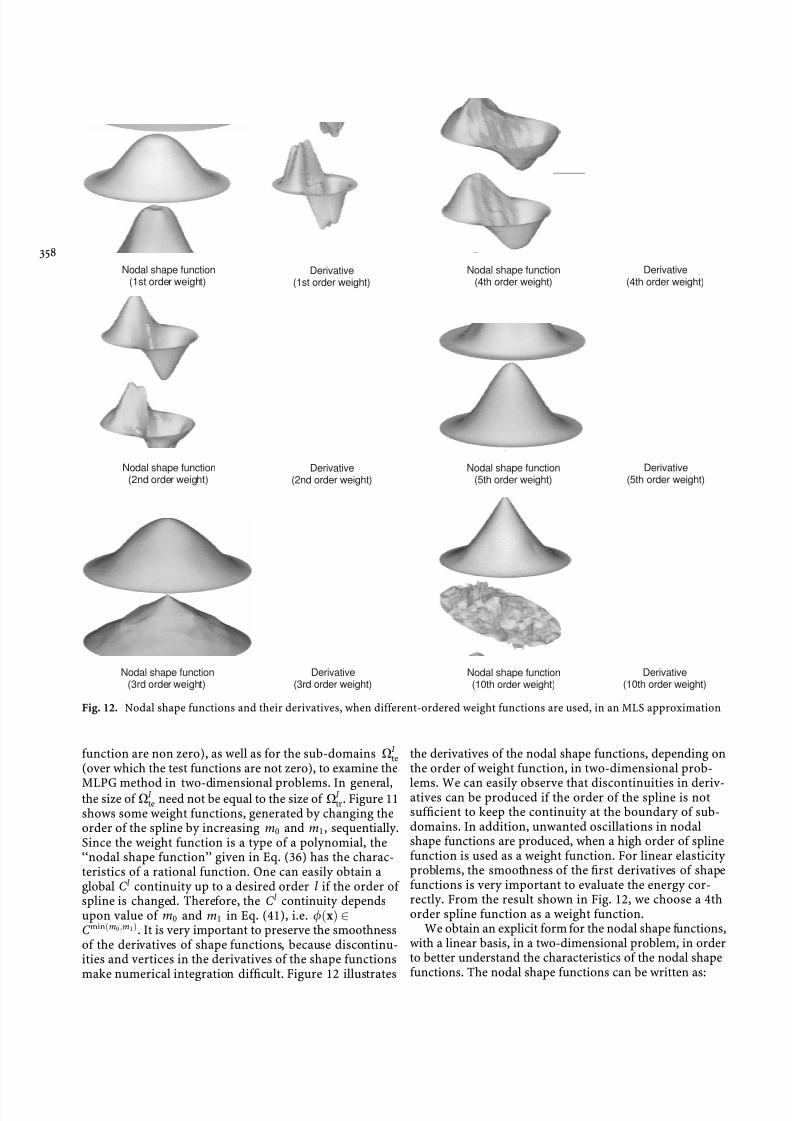
tr . Figure 11shows some weight functions, generated by changing theorder of the spline by increasing m0 and m1, sequentially.Since the weight function is a type of a polynomial, the``nodal shape function'' given in Eq. (36) has the charac-teristics of a rational function. One can easily obtain aglobal C l continuity up to a desired order l if the order of spline is changed. Therefore, the C l continuity dependsupon value of m0 and m1 in Eq. (41), i.e. / x PC min m0Ym1 . It is very important to preserve the smoothnessof the derivatives of shape functions, because discontinu-ities and vertices in the derivatives of the shape functionsmake numerical integration dif®cult. Figure 12 illustrates
the derivatives of the nodal shape functions, depending onthe order of weight function, in two-dimensional prob-
lems. We can easily observe that discontinuities in deriv-atives can be produced if the order of the spline is notsuf®cient to keep the continuity at the boundary of sub-domains. In addition, unwanted oscillations in nodalshape functions are produced, when a high order of splinefunction is used as a weight function. For linear elasticity problems, the smoothness of the ®rst derivatives of shapefunctions is very important to evaluate the energy cor-rectly. From the result shown in Fig. 12, we choose a 4thorder spline function as a weight function.
We obtain an explicit form for the nodal shape functions,with a linear basis, in a two-dimensional problem, in orderto better understand the characteristics of the nodal shapefunctions. The nodal shape functions can be written as:
Nodal shape function(4th order weight)
Nodal shape function(5th order weight)
Nodal shape function(10th order weight)
Derivative(4th order weight)
Derivative(5th order weight)
Derivative(10th order weight)
Nodal shape function(1st order weight)
Nodal shape function(2nd order weight)
Nodal shape function(3rd order weight)
Derivative(1st order weight)
Derivative(2nd order weight)
Derivative(3rd order weight)
Fig. 12. Nodal shape functions and their derivatives, when different-ordered weight functions are used, in an MLS approximation
358

8/6/2019 A Critical Assessment of the Truly Meshless Local Petrov-Galerkin (MLPG),
http://slidepdf.com/reader/full/a-critical-assessment-of-the-truly-meshless-local-petrov-galerkin-mlpg 12/25
/ I xY y wI xY yb xY y
c 0 xY y Yc 1 xY y Yc 2 xY y 1x y
VX
WaY42
where
c 0 xY y a11 xY y a12 xY y xI a13 xY y yI Yc 1 xY y a21 xY y a22 xY y xI a23 xY y yI Yc 2 xY y a31 xY y a32 xY y xI a33 xY y yI Y
a11 xY y N
J 1x2
J w J xY yN
J 1 y2
J w J xY y
ÀN
J 1x J y J w J xY y2 3
2
Y
a12 xY y a21 xY y N
J 1
x J y J w J xY yN
J 1
y J w J xY y
ÀN
J 1x J w J xY y
N
J 1 y2
J w J xY y Y
a13 xY y a31 xY y N
J 1x J w J xY y
N
J 1x J y J w J xY y
ÀN
J 1x2
J w J xY yN
J 1 y J w J xY y Y
a22 xY y N
J 1w J xY y
N
J 1 y2
J w J xY y
ÀN
J 1 y J w J xY y2 3
2
Y
a23 xY y a32 xY y N
J 1x J w J xY y
N
J 1 y J w J xY y
ÀN
J 1w J xY y
N
J 1x J y J w J xY y Y
a33 xY y N
J 1w J xY y
N
J 1x2
J w J xY y
ÀN
J 1x J w J xY y2 3
2Y
b xY y a11 xY yN
J 1w J xY y a12 xY y
N
J 1x J w J xY y
a13 xY yN
J 1 y J w J xY y Y
Equation (42) shows that the shape function has a rationalform. The values of c 0 xY y Yc 1 xY y Yc 2 xY y and b xY ydepend on the location of xY y in the intersection regionsof sub-domains X J
trYJ 1Y2YF F FYN with sub-domains X I
tr
as shown in Fig. 13. This is because of the fact that thevalues of the weight function w J xY y corresponding to thenode J , which control the interpolation at any point xY y ,are different at each xY y in X I Yk
tr , and different numbers of weight functions w J xY y are nonzero at different loca-tions, for example x 1 and x 2 in Fig. 13. In other words, thenodal shape functions / I x consists of a different form of rational function in each small region X I Yk
tr indicated inFig. 13, as:
/ I x k
/ I Yk x Y / I Yk P X I Yktr X 43
Although the smoothness of / I x can be achieved if asuf®cient order of spline function is used as a weightfunction, it is dif®cult to make the shape function / I x tobe a rational polynomial in the sub-domain X I
te . Unfor-tunately, it seems to be impossible to ®nd smooth enoughweight functions possessing the same properties in eachsmall region X I Yk
tr , and this causes a dif®culty in the nu-merical integration of shape functions even if many numbers of Gaussian-quadrature integration points areintroduced.
Requiring that the nodal shape functions be completeonly to represent a globally constant function, i.e. m 1,we obtain the so-called Shepard function (Shepard 1968)given by
/ I 0 x wI x
N J 1 w J x
X 44
The Shepard functions satisfy the zeroth order complete-ness. Although the Shepard shape functions have a simplerstructure than the higher order MLS shape functions, theforms of functions in each small region X I Yk
tr are not thesame. The shape of the Shepard function, which is also arational function, depends on the type of weight function,and the attendant complexity of the nodal shape functionleads to dif®culties in numerical integration. The Shepardfunction in the MLS interpolation is one of the partition of
x 1
x 2
Node I
x 1
x 2
Node I
Fig. 13. The nodal shape function / I x , from MLS interpolation,which is nonzero in X I
tr , has a different form in each small regionX I Yk
tr , which is the intersection of X I tr and X J
tr
3

8/6/2019 A Critical Assessment of the Truly Meshless Local Petrov-Galerkin (MLPG),
http://slidepdf.com/reader/full/a-critical-assessment-of-the-truly-meshless-local-petrov-galerkin-mlpg 13/25
unity functions. The partition of unity (PU) method(Bauska and Melenk 1997) has developed another ap-proximation for meshless methods, by multiplying poly-nomials, such as:
uh x N
I 1
m
j 1
/ I 0 x p j x b jI 45
where p j x are the polynomials, and b jI are the coef®-cients. The consistency in the above shape function de-pends on the order of polynomials. In the MLPGformulation, the above shape function requires an addi-tional degree of freedom, per each node, to be solved for.Duarte and Oden (1996) modify the partition of unity concept, from the MLS shape function of order k, whichthey call the hp-cloud method. The shape function in anhp-cloud method is given by
uh x N
I 1/ I
k x uI m
j 1 p j x b jI 2 3 46
where / I k x is the MLS shape function of order k. The
partition of unity and the hp-cloud methods have alsodifferent characteristics in each small region X I Yk
tr as shownin Fig. 13, because the weight functions in the Shepard andthe MLS shape functions are not the same in each smallregion.
5A simple & elementary method to satisfy essential B.C.exactly; & Interpolation errors in meshless interpolationsIn this section we express the interpolation relation frommeshless approximations such as MLS, Shepard, and PUmethods, in terms of the actual nodal values of the in-terpolant, rather than certain ®ctitious values. As ex-plained before, meshless approximations, in general, donot pass through the nodal data, which are ®ctitious val-ues at nodes. This is the reason why, according to folklorein prior literature (Belytschko et al. 1994; Liu et al. 1995),the essential boundary conditions cannot be imposed di-rectly in meshless methods. However, meshless approxi-mations can be reinterpreted from the point of view of aninterpolation, which passes through the actual nodal val-ues. The schematic description about the interpolation interms of the ®ctitious nodal values uI and the actual nodalvalues ~uI uI is shown in Fig. 14. We now derive the
relation between the ®ctitious nodal values uI
and theactual nodal values ~uI to impose the essential boundary conditions directly. Consider the following meshless ap-proximation:
~u x N
I 1/ I x uI 47
such that
~u J N
I 1/ I x J uI 48
where ~u J are the actual nodal values at nodes J , i.e. ~u J u J ,of the interpolant ~u x . Then we have:
uI N
J 1RIJ ~u J 49
withRIJ / J x I Â Ã
À1 X 50
The transformation matrix RIJ in Eq. (50) can be obtainedexplicitly, because the nodal shape functions / I can besimply evaluated at the nodes in the domain. Therefore, itis possible that a meshless approximation can be reinter-preted by using the nodal values ~uI , as:
~u x N
I 1
N
J 1/ I x RIJ ~u J
N
J 1u J x ~u J 51
where u J x de®ned in Eq. (51) have the property that
u J
x I d JI . The above Eq. (51) only involves a lineartransformation RIJ form the ®ctitious nodal values uI tothe actual nodal values ~uI . Thus, the essential boundary conditions may be easily imposed in meshless methods, by using this linear transformation. If the discretized globalsystem of equations can be written, the ®ctitious nodalvalues u J as:
N
J 1KIJ u J f I X 52
Then, the global system of equation for the actual nodalvalues ~u J may be written as:
N
J 1~KIJ ~u J f I 53
where
~KIJ
N
K 1KIK RKJ 54
In the above equation, RKJ is the transformation matrix inmulti-dimensional space. On the other hand, if the testfunctions are also rewritten as:
~v x N
I 1wI x vI
N
I 1
N
J 1wI x T IJ ~v J 55
Interpolation
Node I
Exact function u(x)
ûI ~u = uI I
Fig. 14. An illustration of `interpolation' in meshless schemes.uI is the ®ctitious nodal data at node I and ~uI is the exactnodal values at node I for interpolation
360
8/6/2019 A Critical Assessment of the Truly Meshless Local Petrov-Galerkin (MLPG),
http://slidepdf.com/reader/full/a-critical-assessment-of-the-truly-meshless-local-petrov-galerkin-mlpg 14/25
where wI x are the nodal test shape functions, and
T IJ w J x I Â ÃÀ1 X 56
Then the global system of equations can be recast by N
J 1
~~KIJ ~u J ~f I 57
where
~~KIJ
N
K 1
N
L 1TÀ1
IK KKL RLJ and ~f I N
J 1TÀ1
IJ f J X
58
In the above equations, TIJ is the transformation matrix inmulti-dimensional space based on the nodal test functionswI x , and KKL and f J are given in Eq. (23). Although thebandwidth of the stiffness matrix ~KIJ or
~~KIJ in either Eq.(54) or Eq. (58) is larger than that of the original stiffnessmatrix KIJ , we can directly impose the essential boundary conditions in the transformed Eq. (53) or Eq. (57).Moreover, the size of stiffness matrix ~KIJ or
~~KIJ in thisapproach may not cause a serious problem, because thereare many re®ned techniques for solving the simultaneouslinear equations. Note that the following properties hold:
N
I 1
N
J 1/ I x RIJ 1 Y 59a
N
I 1
N
J 1/ I x RIJ x J
À Áq x qY q m X
To impose the essential boundary conditions, we do not,
in general, need to transform all ®ctitious nodal values uI
to the actual nodal values ~uI . In order to circumventcomputational burden for dealing with a large size of thestiffness matrix, only a partial transformation involvingdata close to the boundary may be used, as:
~u"I
È ÉuI f g& ' / J x"I dIJ !u J
È É 60
where "I denotes the nodes with prescribed essential boun-dary conditions. The remainders of procedures, using thistransformation (60) are the same for the case of a fulltransformation explained in the above. As a result, we caneasily and exactly impose the essential boundary conditions
using this transformation technique. The numerical results,in Sect. 7, obtained with this method to impose the essentialboundary conditions show very satisfactory results.
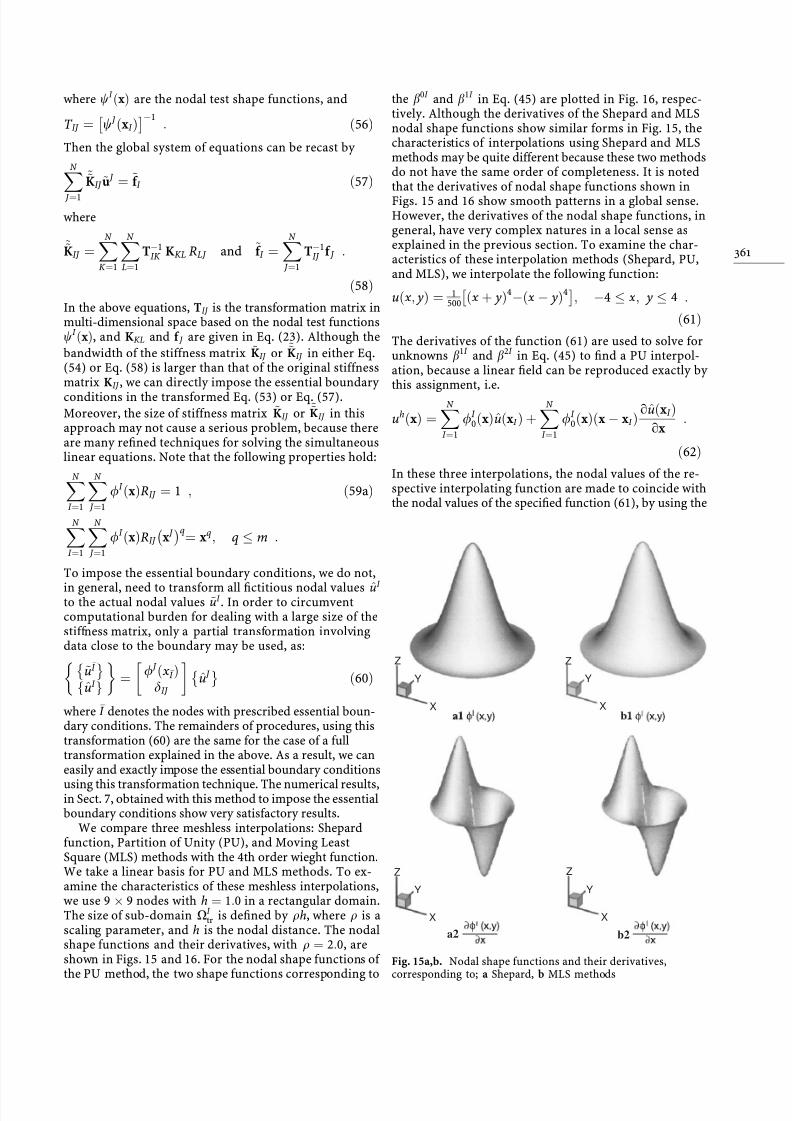
We compare three meshless interpolations: Shepardfunction, Partition of Unity (PU), and Moving LeastSquare (MLS) methods with the 4th order wieght function.We take a linear basis for PU and MLS methods. To ex-amine the characteristics of these meshless interpolations,we use 9 Â 9 nodes with h 1X0 in a rectangular domain.The size of sub-domain X I
tr is de®ned by qh, where q is ascaling parameter, and h is the nodal distance. The nodalshape functions and their derivatives, with q 2X0, areshown in Figs. 15 and 16. For the nodal shape functions of the PU method, the two shape functions corresponding to
the b0I and b1I in Eq. (45) are plotted in Fig. 16, respec-tively. Although the derivatives of the Shepard and MLSnodal shape functions show similar forms in Fig. 15, thecharacteristics of interpolations using Shepard and MLSmethods may be quite different because these two methodsdo not have the same order of completeness. It is notedthat the derivatives of nodal shape functions shown inFigs. 15 and 16 show smooth patterns in a global sense.However, the derivatives of the nodal shape functions, ingeneral, have very complex natures in a local sense asexplained in the previous section. To examine the char-acteristics of these interpolation methods (Shepard, PU,and MLS), we interpolate the following function:
u xY y 1500 x y 4À x À y 4
 ÃY À4 xYy 4 X61
The derivatives of the function (61) are used to solve forunknowns b1I and b2I in Eq. (45) to ®nd a PU interpol-ation, because a linear ®eld can be reproduced exactly by this assignment, i.e.
uh x N
I 1/ I
0 x u x I N
I 1/ I
0 x x À x I o u x I
o x X
62
In these three interpolations, the nodal values of the re-spective interpolating function are made to coincide withthe nodal values of the speci®ed function (61), by using the
a2 b2
Y
X
Z
Y
X
Z
Y
X
Z
Y
X
Z
Fig. 15a,b. Nodal shape functions and their derivatives,corresponding to; a Shepard, b MLS methods
3

8/6/2019 A Critical Assessment of the Truly Meshless Local Petrov-Galerkin (MLPG),
http://slidepdf.com/reader/full/a-critical-assessment-of-the-truly-meshless-local-petrov-galerkin-mlpg 15/25
transformation (49) to rede®ne the undetermined param-eters in these interpolations in terms of the actual nodalvalues. For the PU interpolation, the derivatives of inter-polations also coincide with the derivatives of the givenfunction (61) because the derivatives of the function (61)are assigned to ®nd the relation between b jI and ~b jI inEq. (45).
In these analyses, we use two sizes of sub-domains:q 2X0 and q 3X0. In Fig. 17, the interpolations for u x ,using the three methods (Shepard, PU, and MLS), show good agreements with the exact function, even thoughsmall oscillations or indentations are observed. In fact, thederivatives of interpolations are important to examine thecharacteristics of methods, because derivatives of thenodal shape functions are directly related with the inte-grand for the global stiffness matrix. Figure 18 shows theunwanted waves in the derivatives of interpolations usingthese methods for the cases of q 2X0 and q 3X0.Compared to the interpolations in Fig. 17, the derivativesof interpolations have relatively large oscillations or in-
dentations. It should be noted that a smaller size of thesub-domains may induce larger oscillations or indenta-tions, in the nodal shape functions derived from meshlessinterpolations. Particularly, the derivatives of interpolat-ions using the PU method show larger oscillations or in-dentations than those in the other meshless interpolations.These characteristics of the interpolations are directly re-lated to the dif®culties in the numerical integration for theglobal stiffness matrix.
Next, the interpolation errors in meshless interpolat-ions are studied by numerical approaches. Since themeshless interpolations satisfy the completeness condi-
a2 b2
Y
X
Z
Y
X
Z
Y
X
Z
Y
X
Z
Fig. 16a,b. Nodal shape functions and their derivatives,corresponding to PU; a the ®rst nodal shape function,b the second nodal shape function
a b c
d e f
Y
X
ZY
X
Z
Y
X
Z
Y
X
ZY
X
ZY
X
Z
a b c
d e f
Y
X
ZY
X
Z
Y
X
Z
Y
X
ZY
X
ZY
X
ZFig. 17a±f. Meshless interpol-ations for u xY y using aShepard q 2X0 , b PUq 2X0 , c MLS q 2X0 , d
Shepard q 3X0 , e PUq 3X0 , f MLS q 3X0
362

8/6/2019 A Critical Assessment of the Truly Meshless Local Petrov-Galerkin (MLPG),
http://slidepdf.com/reader/full/a-critical-assessment-of-the-truly-meshless-local-petrov-galerkin-mlpg 16/25
tions, given in Eq. (59), the shape functions based on theseinterpolations give convergent characteristics. In otherwords, the numerical solutions for a partial differentialequation should converge to exact solutions as the nodaldistance tends to zero. Therefore, the errors in numericalresults in the MLPG method will depend on the inter-polation errors. The best approximation theorem may enable us to have an error estimate for elliptic boundary-value problems. In meshless interpolations, the rates of convergence may depend upon the nodal distance h aswell as the size of sub-domain de®ned by qh, where q isthe scaling parameter for the size of sub-domain X I
tr .Supposing that the interpolation-error-estimate may havethe h-convergence as in Galerkin ®nite elements, the fol-lowing interpolation-error-estimate may be assumed to bepreserved:
u À ~uk kk GqYk hm 1Àk uj jm 1 63
where GqYk is a function of q and k, Ák kk is the norm in theSobolev space, and m indicates the order of the completepolynomial in the interpolation function. In our numericalanalyses, we show the tendencies of interpolation errors inmeshless interpolation through a numerical approach.
The function (61) is used to examine the characteristicsof interpolation using meshless interpolations. In ourcomputations, the linear transformation (49) and the MLSinterpolation with 4th order weight functions are used tointerpolate the function (61). We use the relative error r 1for H 1-norm de®ned by
r 1u À ~uk k1
uk k1X 64
We change two parameters; nodal distance h and thescaling parameter q for the size of sub-domain X I
tr . Asshown in Fig. 19, the rates of convergence for the inter-polation errors show linear relationships in a logarithmicscale, which means that Eq. (63) represents a good relationbetween the interpolation errors and the nodal distance. Itshould be noted that the rates of convergence in these
a b c
e
Y
X
Z
Y
X
Z
Y
X
Z
d
Y
X
Z
Y
X
Z
Y
X
Z
f
Fig. 18a±f. The derivatives of meshless interpolations foru xY y using a Shepardq 2X0 , b PU q 2X0 ,
c MLS q 2X0 , d Shepardq 3X0 , e PU q 3X0 ,
f MLS q 3X0
0
-0.5
-1.0
-1.5
-2.0
-2.5
-3.0-0.4 -0.3 -0.2 -0.1 0 0.1 0.2 0.3 0.4
Log (h)10
L o g
( r
)
1 0
1
ρ
ρ
ρ
= 2.0= 2.5
= 3.0
0
-0.5
-1.0
-1.5
-2.0
-2.5
-3.0-0.4 -0.3 -0.2 -0.1 0 0.1 0.2 0.3 0.4
Log (h)10
L o g
( r
)
1 0
1
ρ
ρ
ρ
= 2.0= 2.5
= 3.0
Fig. 19. Convergence of the interpolation error (energy- norm)with nodal distance, for different sizes of the sub-domain X I
tr
3
8/6/2019 A Critical Assessment of the Truly Meshless Local Petrov-Galerkin (MLPG),
http://slidepdf.com/reader/full/a-critical-assessment-of-the-truly-meshless-local-petrov-galerkin-mlpg 17/25
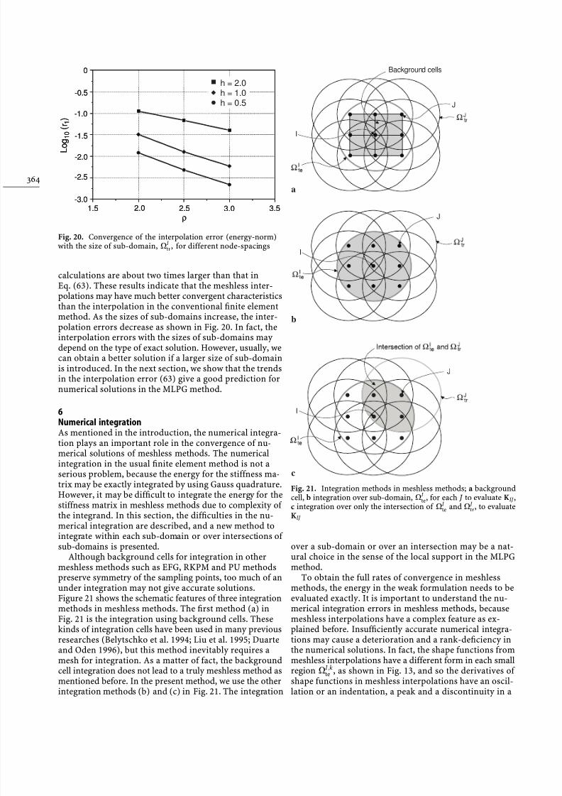
calculations are about two times larger than that inEq. (63). These results indicate that the meshless inter-polations may have much better convergent characteristicsthan the interpolation in the conventional ®nite elementmethod. As the sizes of sub-domains increase, the inter-polation errors decrease as shown in Fig. 20. In fact, theinterpolation errors with the sizes of sub-domains may depend on the type of exact solution. However, usually, wecan obtain a better solution if a larger size of sub-domainis introduced. In the next section, we show that the trendsin the interpolation error (63) give a good prediction fornumerical solutions in the MLPG method.
6Numerical integrationAs mentioned in the introduction, the numerical integra-tion plays an important role in the convergence of nu-merical solutions of meshless methods. The numericalintegration in the usual ®nite element method is not aserious problem, because the energy for the stiffness ma-trix may be exactly integrated by using Gauss quadrature.However, it may be dif®cult to integrate the energy for thestiffness matrix in meshless methods due to complexity of the integrand. In this section, the dif®culties in the nu-merical integration are described, and a new method tointegrate within each sub-domain or over intersections of sub-domains is presented.
Although background cells for integration in othermeshless methods such as EFG, RKPM and PU methodspreserve symmetry of the sampling points, too much of anunder integration may not give accurate solutions.Figure 21 shows the schematic features of three integrationmethods in meshless methods. The ®rst method (a) inFig. 21 is the integration using background cells. Thesekinds of integration cells have been used in many previousresearches (Belytschko et al. 1994; Liu et al. 1995; Duarteand Oden 1996), but this method inevitably requires amesh for integration. As a matter of fact, the backgroundcell integration does not lead to a truly meshless method asmentioned before. In the present method, we use the otherintegration methods (b) and (c) in Fig. 21. The integration
over a sub-domain or over an intersection may be a nat-
ural choice in the sense of the local support in the MLPGmethod.To obtain the full rates of convergence in meshless
methods, the energy in the weak formulation needs to beevaluated exactly. It is important to understand the nu-merical integration errors in meshless methods, becausemeshless interpolations have a complex feature as ex-plained before. Insuf®ciently accurate numerical integra-tions may cause a deterioration and a rank-de®ciency inthe numerical solutions. In fact, the shape functions frommeshless interpolations have a different form in each smallregion X I Yk
te , as shown in Fig. 13, and so the derivatives of shape functions in meshless interpolations have an oscil-lation or an indentation, a peak and a discontinuity in a
L o g
( r
)
1 0
1
0
-0.5
-1.0
-1.5
-2.0
-2.5
-3.01.5 2.0 2.5 3.0 3.5
ρ
h = 2.0h = 1.0h = 0.5
L o g
( r
)
1 0
1
0
-0.5
-1.0
-1.5
-2.0
-2.5
-3.01.5 2.0 2.5 3.0 3.5
ρ
h = 2.0h = 1.0h = 0.5
Fig. 20. Convergence of the interpolation error (energy-norm)with the size of sub-domain, X I
tr , for different node-spacings
a
b
c
Background cells
I
I
I
J
J
J
Fig. 21. Integration methods in meshless methods; a backgroundcell, b integration over sub-domain, X I
te, for each J to evaluate KIJ ,c integration over only the intersection of X I
te and X J tr , to evaluate
KIJ
364

8/6/2019 A Critical Assessment of the Truly Meshless Local Petrov-Galerkin (MLPG),
http://slidepdf.com/reader/full/a-critical-assessment-of-the-truly-meshless-local-petrov-galerkin-mlpg 18/25
local sense. Furthermore, rational polynomials used as abasis, and the chosen weight functions, produce complexforms of nodal shape functions in the sub-domains X I
te.Considering the fact that the shape functions based onmeshless interpolations are not simple polynomials, it may not be desirable to integrate over the whole area of a sub-domain X I
teeach time, using simple Gaussian quadrature,
as shown in Fig. 21b, to obtain each KIJ for each value of J whose X J
tr intersects only partially with X I te . In fact, it may
be necessary to recourse to a numerical quadrature sepa-rately in each small region X I Yk
te , as shown in Fig. 13. Itseems to be impossible to divide domains for integrationwith alignments of the boundaries of the small regionsX I Yk
te , as shown in Fig. 13. Moreover, we found throughnumerical experiments that many small partitions in adomain of integration, such as a sub-domain X I
te , or evenan intersection of X I
te and X J tr , give better solutions, than in
the cases of integrating over a whole domain of integrationwith a large number of integration points. Therefore, weuse small partitions distributed in the domain of integra-
tion. The other dif®culty in the integration for two-di-mensional or three-dimensional problems is to integrateover the region intersecting with the global boundaries,which produces polygonal shapes of intersection, for in-tegration, as shown in Fig. 22. One possible way to inte-grate these kinds of geometry, enclosed by circular arcsand straight lines, is to use a transformation from thedomain of integration into a unit circle, which is a one-to-one and nonsingular transformation. The point n on a unitcircle is de®ned by
nx À x 0x 1 À x 0j j
65
where x 0 is the nodal position or the center of intersection,and x 1 is a position at the boundary of a sub-domain or anintersection to the direction x À x 0, as shown in Fig. 22.The small partitions for integration are divided regularly on a unit-circle. This algorithm can be extended to three-dimensional problems along the same lines. Hence, theintegration in the sub-domain X I
tecan be written as: X I
te
f x dX X c
f à n J dX à 66
where J is the Jacobian corresponding to the coordinatetransformation, and X c indicates a unit circle. Then thenumerical integration becomes:
X I te
f x dX M
k 1
nl
l 1 Al J l f Ãl 2 3
k
R M 67
where M denotes the total number of partitions for inte-gration, Al are the weights for numerical integration, andR M is the error for the numerical integration in the sub-domain X I
te. The integration for an intersection of X I
teand
X J tr can be evaluated by the same procedures. The inte-
gration error R M depends on the number of partitions andintegration points, and on the characteristics of shapefunctions, such as the size of sub-domain X I
te and the typeof weight function wI x . If there is a discontinuity or avertex in the nodal shape functions in X I
te , the integrationerror increases, because a polynomial approximation im-plicit in the Gaussian integration produces mismatchesbetween the nodal shape function in X I
te , and an approx-imation for integration. In this paper, we use circles andellipses as the shapes of sub-domains X I
te ; an investigationof the case of rectangular sub-domains for X I
te will bepresented in our forthcoming papers.
To examine the effect of the types of weight functions,the numerical integration inside a generic intersection of X I
te and X J tr is performed by using Gaussian quadrature.
The following is a generic integrand in the evaluation of the local weak form in X I
te , when the nodal trial functionand nodal test functions are identical:
E1o / I xY y
o xo / J xY y
o xo / I xY y
o yo / J xY y
o yY
68a
E2o / I xY y
o xo / J xY y
o yo / I xY y
o yo / J xY y
o xX
68bFigure 23 shows the shapes of the integrands E1 and E2,arising from the MLS interpolation in a sub-domain, forthe case when I J in Eqs. (68a) and (68b). We change theorder of weight function wI x to observe the shapes of integrands E1 and E2 in the stiffness matrix of MLPGformulation. From these ®gures, it is clear that a numericalintegration may be very dif®cult if a proper order of theweight function is not chosen. As explained in the Sect. 4,we choose a 4th order weight function, in order to givesmoothness to the derivatives of the shape functions.However, small oscillations or indentations in the deriva-tive of the shape functions, due to different forms of
a
b
Unit circle
Unit circle
Mapping
Mapping
Partitions
Partitions
Boundary
Boundary
x1
x1
x0
x0
Node I
Sub-domain
Sub-domains
Intersection
a
b
Unit circle
Unit circle
Mapping
Mapping
Partitions
Partitions
Boundary
Boundary
x1
x1
x0
x0
Node I
Sub-domain
Sub-domains
Intersection
Fig. 22a,b. Mapping onto a unit-circle ( a) from a sub-domain X I te
and ( b) from an intersection of X I te and X J
tr . x 0 is the center of sub-domain or intersection, and x 1 is the point at the boundary
3

8/6/2019 A Critical Assessment of the Truly Meshless Local Petrov-Galerkin (MLPG),
http://slidepdf.com/reader/full/a-critical-assessment-of-the-truly-meshless-local-petrov-galerkin-mlpg 19/25
functions in each small region as shown in Fig. 13, forcethe numerical integration process to require many parti-tions and integration points. We examine the convergenceof integration for a generic intersection region shown inFig. 24. The shapes of the integrands E1 and E2 in theregion of intersection between X I
te and X J tr are shown in
Fig. 25. The exact integration is assumed to be a value
obtained by using a trapzoidal integration with 400 Â 1200points. Figure 26 shows the convergence of integration of E1 and E2 by using Gaussian quadrature, with partitions.In this calculation, we use 3 Â 3 integration points for eachpartition, and the number of partitions along the radialdirection in a unit-circle is varied. The numerical inte-gration does not show uniform convergence, as the num-ber of partitions increases, which may be due to thecomplexity of shape functions. However, we can say thatthe errors in numerical integrations decrease, albeit with a¯uctuation, as the number of partitions increases. There-fore, integration with partitions may be a proper approachto evaluate energy for the stiffness matrix, in the presentPetrov-Galerkin formulation.
7Numerical experimentsThe numerical results of the MLPG method as applied toproblems in two-dimensional elasto-statics, speci®cally acantilever beam and a plate with a hole as shown in Fig. 27,are now discussed. The Young modulus and the Poisson's
E1 (1st order weight)
E1 (2nd order weight)
E1 (3rd order weight) E2 (3rd order weight)
E2 (2nd order weight)
E2 (1st order weight) E1 (4th order weight)
E1 (5th order weight)
E1 (10th order weight) E2 (10th order weight)
E2 (5th order weight)
E2 (4th order weight)E1 (1st order weight)
E1 (2nd order weight)
E1 (3rd order weight) E2 (3rd order weight)
E2 (2nd order weight)
E2 (1st order weight) E1 (4th order weight)
E1 (5th order weight)
E1 (10th order weight) E2 (10th order weight)
E2 (5th order weight)
E2 (4th order weight)
Fig. 23. The shapes of E1 and E2 with changing the order of weight functions. MLS shape functions are used
Node J
Node I
Fig. 24. Intersection for two sub-domains X I te and X J
tr
366

8/6/2019 A Critical Assessment of the Truly Meshless Local Petrov-Galerkin (MLPG),
http://slidepdf.com/reader/full/a-critical-assessment-of-the-truly-meshless-local-petrov-galerkin-mlpg 20/25
ratio are E 1X0 Â 1010 and m 0X25, respectively. Thepenalty parameter chosen in the analyses isa 1X0 Â 105 E, and the new method, using transforma-tion from ®ctitious nodal values to actual nodal values, forimposing the essential boundary conditions is also im-plemented for some examples. We perform numerical in-
tegration either in the entire X I te each time, or only in an
intersection of X I te and X J
tr ; and in each case, partitions areused, as explained before. In our computations, the body forces bi in Eq. (1) are set to be zero. We use the energy norm de®ned as:
ek k 12 X
e TDe dX
12
X 69
The relative error for ek k is de®ned as:
r ee exact À e numk k
e exactk kX 70
7.1Cantilever beamWe ®rst consider a cantilever beam problem as shown inFig. 27a. The exact solution for this problem is given inTimoshenko and Goodier (1970) as:
u1 ÀP
6EI y ÀD2 3x 2LÀ x 2 m y yÀ D Y
71a
u2P
6EI 4x2 3LÀ x 3mLÀ x y ÀD2
2 4 5m4
D2x571b
where
I D3
12X
The stresses corresponding to the above are
0
-0.05
-0.10
E 1
2 3 45 6
23
4Y
X
56
a
b
0
-0.05
-0.10
23
45
6X 2
34
5
6
Y
E 2
Fig. 25a,b. The shapes of E1 and E2 in a sub-domain X I te inter-
secting with another sub-domain X J tr , as shown in Fig. 24
0
-1
-2
-3
-4
-5
-6
-71 2 3 4 5 6 7 8
Number of partitions along radial direction
L o g 1 0
( )
r
EE
1
2
Fig. 26. The relative errors in numerical integrations forE1 and E2
x1
x1
x2
x2
a
a
b
L
PD u-
Fig. 27a,b. Geometric description for numerical experiments;a a cantilever beam, b a plate with a hole
3

8/6/2019 A Critical Assessment of the Truly Meshless Local Petrov-Galerkin (MLPG),
http://slidepdf.com/reader/full/a-critical-assessment-of-the-truly-meshless-local-petrov-galerkin-mlpg 21/25
r 11 ÀP I
L À x y ÀD2 Y 72a
r 22 0 Y 72b
r 12 À Py2I
y À D X 72c
We use regularly distributed 24 (6 Â 4), 77 (11 Â 7), 160(16 Â 10) and 273 (21 Â 13) nodes for a model withL 5X0 and D 3X0. Integration only over the intersec-tions of X I
te and X J tr , along with partitions, is used to solve
this problem; and 3 Â 3 Gaussian quadrature is used tointegrate the energy in each small partition. The nodalshape functions in these examples are taken from the MLSinterpolations with 4th order weight functions. We reporthere results for various values of the number of partitions,various values of the sizes of sub-domain X I
teX J
tr , andvarious values of the nodal distances. As the nodal dis-tance h decreases, for the scaling parameters of radius of X I
te of q 2X0 and q 3X0, the relative errors for the en-
ergy norm decrease as shown in Fig. 28. It is observedfrom this ®gure that a monotonic convergence cannot beobtained if suf®cient numbers of partitions are not intro-duced. Particularly, the numerical solutions deteriorate asthe nodal distance decreases, if the numerical integrationis not accurate enough to evaluate the energy for thestiffness matrix. In other words, the more nodes are addedin the domain, the more partitions or integration pointsare required to achieve the accuracy corresponding to asmaller nodal distance. These kinds of dif®culties arecaused by the complexity of the shape functions inmeshless methods. It should be noted that the rates of convergence in these numerical examples are about 2.0,which is higher than the value in the Galerkin ®nite ele-ment method. The effect of the size of sub-domain isshown in Fig. 29, in which the relative errors for the energy norm decrease as the size of sub-domain X I
teX J
tr in-creases. This trend is similar to the results for the inter-polation-error-estimate in Sect. 6 (see Fig. 20). The
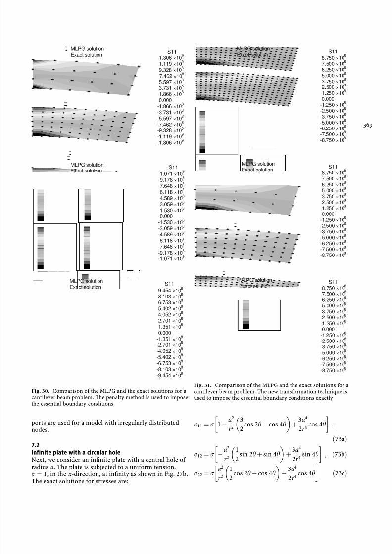
comparison of numerical and exact deformations, as wellas stress distributions r 11, are shown in Fig. 30. In theprevious examples, we used the penalty parameter tech-nique to impose the essential boundary conditions. As asimple and elementary method introduced in Sect. 6 toimpose the essential boundary conditions, the new methodusing linear transformation is applied to these examples.The MLPG solutions with this method of enforcing theessential boundary conditions show very satisfactory re-sults as shown in Fig. 31. We also change the nodal shapefunctions corresponding to the Shepard and partition of unity interpolations. As explained in Sect. 4, the Shepardshape function is the most simple shape function in theMLS interpolation. Therefore, the numerical results with3 Â 12 and 6 Â 24 partitions are similar, as shown inFig. 32, which implies that the numerical integration forShepard function is much easier than for a MLS function.This advantage is due to the simpliticity of the shapefunction, which makes numerical integration easier.However, the relative errors for the energy norm are large,
and the rates of convergence are slow. Figure 33 shows theresults with partition of unity interpolations, in which thenumerical solutions using small number of partitions(3 Â 12 partitions) do not converge as the nodal distancedecreases.
We examine a long beam example, to investigate theeffect of the shape of sub-domain X I
teX J
tr for threemodels having different nodal distances in the x- and y-directions, as shown in Fig. 34. In these analyses, we usesub-domain integration with partitions as shown in Fig.22a. The beam dimensions are L 40X0 and D 4X0. Wechange the shape of the sub-domain to ellipses, by ad- justing the nodal distances in the x- and y-directions. Theresults are shown in Fig. 35, in which the relative errors forthe energy norm for elliptical supports X J
tr are lower thanthe errors in the cases with circular supports X J
tr . In this®gure, h1 indicates nodal distance in the x-direction. It isobserved from these results that the quality of the nu-merical solutions may be improved, when elliptical sup-
0
-0.5
-1.0
-1.5
-2.0
-2.5
-3.0
L o g
( r )
1 0
e
Log (h)10
-0.7 -0.6 -0.5 -0.4 -0.3 -0.2 -0.1 0 0.1
= 2.0, 3x12 partitions= 2.0, 6x24 partitions= 3.0, 3x12 partitions= 3.0, 6x24 partitions
Fig. 28. Rates of convergence of the energy norm in the problemof a cantilever beam, with nodal spacing, for different sizes of X J
te
0
-0.5
-1.0
-1.5
-2.0
-2.5
-3.0
L o g
( r )
1 0
e
1.5 2.0 2.5 3.0 3.5
24 nodes77 nodes
273 nodes
Fig. 29. Rates of convergence of the energy norm in theproblem of a cantilever beam, with the size of X J
te , for differentnodal spacing 6 Â 24 partitions are used for numericalintegration
368
8/6/2019 A Critical Assessment of the Truly Meshless Local Petrov-Galerkin (MLPG),
http://slidepdf.com/reader/full/a-critical-assessment-of-the-truly-meshless-local-petrov-galerkin-mlpg 22/25
ports are used for a model with irregularly distributednodes.
7.2Infinite plate with a circular holeNext, we consider an in®nite plate with a central hole of radius a. The plate is subjected to a uniform tension,r 1, in the x-direction, at in®nity as shown in Fig. 27b.The exact solutions for stresses are:
r 11 r 1 Àa2
r 232
cos 2h cos 4h 3a4
2r 4cos 4h !Y
73a
r 12 r Àa2
r 212
sin 2h sin 4h 3a4
2r 4sin 4h !Y 73b
r 22 ra2
r 212
cos 2h À cos 4h
À
3a4
2r 4cos 4h
!73c
MLPG solutionExact solution
MLPG solutionExact solution
MLPG solutionExact solution S11
1.306 ×10 9
1.119 ×10⁹
9.328 ×10 8
7.462 ×10 8
5.597 ×10 8
3.731 ×10 8
1.866 ×10⁸
0.000-1.866 ×10 8
-3.731 ×10 8
-5.597 ×10 8
-7.462 ×10 8
-9.328 ×10 8
-1.119 ×10 9
-1.306 ×10 9
S111.071 ×10 9
9.178 ×10 8
7.648 ×10 8
6.118 ×10⁸
4.589 ×10 8
3.059 ×10 8
1.530 ×10 8
0.000-1.530 ×10 8
-3.059 ×10 8
-4.589 ×10 8
-6.118 ×10 8
-7.648 ×10 8
-9.178 ×10 8
-1.071 ×10 9
S11
9.454 ×10⁸
8.103 ×10 8
6.753 ×10 8
5.402 ×10 8
4.052 ×10 8
2.701 ×10 8
1.351 ×10 8
0.000-1.351 ×10 8
-2.701 ×10 8
-4.052 ×10 8
-5.402 ×10 8
-6.753 ×10 8
-8.103 ×10 8
-9.454 ×10 8
Fig. 30. Comparison of the MLPG and the exact solutions for acantilever beam problem. The penalty method is used to imposethe essential boundary conditions
MLPG solutionExact solution
MLPG solutionExact solution
MLPG solutionExact solution
S118.750 ×10 8
7.500 ×10 8
6.250 ×10 8
5.000 ×10 8
3.750 ×10 8
2.500 ×10 8
1.250 ×10 8
0.000-1.250 ×10 8
-2.500 ×10 8
-3.750 ×10 8
-5.000 ×10 8
-6.250 ×10 8
-7.500 ×10 8
-8.750 ×10 8
S118.750 ×10 8
7.500 ×10 8
6.250 ×10 8
5.000 ×10 8
3.750 ×10 8
2.500 ×10 8
1.250 ×10 8
0.000-1.250 ×10 8
-2.500 ×10 8
-3.750 ×10 8
-5.000 ×10 8
-6.250 ×10 8
-7.500 ×10 8
-8.750 ×10 8
S118.750 ×10 8
7.500 ×10 8
6.250 ×10 8
5.000 ×10 8
3.750 ×10 8
2.500 ×10 8
1.250 ×10 8
0.000-1.250 ×10 8
-2.500 ×10 8
-3.750 ×10 8
-5.000 ×10 8
-6.250 ×10 8
-7.500 ×10 8
-8.750 ×10 8
Fig. 31. Comparison of the MLPG and the exact solutions for acantilever beam problem. The new transformation technique isused to impose the essential boundary conditions exactly
3

8/6/2019 A Critical Assessment of the Truly Meshless Local Petrov-Galerkin (MLPG),
http://slidepdf.com/reader/full/a-critical-assessment-of-the-truly-meshless-local-petrov-galerkin-mlpg 23/25
where r Yh are the polar coordinates, and h is measuredfrom the positive x-axis in a counterclockwise direction.The corresponding displacements, in the plane strain case,
are given by
u11 m
Er 2 1
1 mr cos h
21 m
a2
r cos h
12
a2
r cos 3h
12
a4
r 3cos 3h3Y 74a
u21 m
Er 2À
m1 m
r sin h À1 À m1 m
a2
r sin h
12
a2
r sin 3h À
12
a4
r 3sin 3h3X 74b
Due to symmetry, only a part, 0 x 4 and 0 y 4,of the upper right quadrant of the plate is modeled asshown in Fig. 27b. Symmetry conditions are imposed on
L o g
( r
)
1 0
e
Log (h)10
-0.7 -0.6 -0.5 -0.4 -0.3 -0.2 -0.1 0 0.1
0.5
0
-0.5
-1.0
-1.5
-2.0
ρ = 2.0, 3x12 partitions
ρ = 2.0, 6x24 partitions
ρ = 3.0, 3x12 partitions
ρ = 3.0, 6x24 partitions
Fig. 32. Rates of convergence of the energy norm, with nodalspacing, using Shepard functions, in a cantilever beam problem
L o g
( r )
1 0
e
Log (h)10
-0.7 -0.6 -0.5 -0.4 -0.3 -0.2 -0.1 0 0.1
3
2
1
0
-1
-2
-3
= 2.0, 3x12 partitions= 2.0, 6x24 partitions= 2.0, 12x48 partitions= 3.0, 3x12 partitions= 3.0, 6x24 partitions= 3.0, 12x48 partitions
+
+
Fig. 33. Rates of convergence of the energy norm, with nodalspacing, using partition of unity shape functions, in a cantileverbeam problem
MLPG solutionExact solution
MLPG solutionExact solution
MLPG solutionExact solution
S115.294 ×10 8
4.538 ×10 8
3.782 ×10 8
3.025 ×10 8
2.269 ×10 8
1.513 ×10 8
7.563 ×10 7
0.000-7.563 ×10 7
-1.513 ×10 8
-2.269 ×10 8
-3.025 ×10 8
-3.782 ×10 8
-4.538 ×10 8
-5.294 ×10 8
S11
5.582 ×10⁸
4.785 ×10 8
3.987 ×10 8
3.190 ×10 8
2.392 ×10 8
1.595 ×10 8
7.975 ×10 7
0.000-7.975 ×10 7
-1.595 ×10 8
-2.392 ×10 8
-3.190 ×10 8
-3.987 ×10 8
-4.785 ×10 8
-5.582 ×10 8
S115.250 ×10 8
4.500 ×10 8
3.750 ×10 8
3.000 ×10 8
2.250 ×10 8
1.500 ×10 8
7.500 ×10 7
0.000-7.500 ×10 7
-1.500 ×10 8
-2.250 ×10 8
-3.000 ×10 8
-3.750 ×10 8
-4.500 ×10 8
-5.250 ×10 8
Fig. 34. A Comparison of the MLPG and the exact solutions for along cantilever beam, using elliptical supports
370

8/6/2019 A Critical Assessment of the Truly Meshless Local Petrov-Galerkin (MLPG),
http://slidepdf.com/reader/full/a-critical-assessment-of-the-truly-meshless-local-petrov-galerkin-mlpg 24/25
the left and bottom edges, i.e. u1 0, t 2 0 is prescribedon the left edge and u2 0, t 1 0 on the bottom edge, andthe inner boundary at a 1 is traction free. The tractionboundary conditions, as given by the exact solutions, areimposed on the right ( x 4) and top ( y 4) edges. Thesub-domain integration with partitions, as shown inFig. 22a is used to evaluate the energy for the stiffnessmatrix. We use three models as shown in Fig. 36 to observethe rates of convergence using circular as well as ellipticalsub-domains X I
tr . Figure 36 compares the MLPG and theexact solutions, for the stress distribution r 11, when el-liptical supports are used. Similar to the cantilever beamproblem, the relative errors for the energy norm are lowerfor elliptical supports than in the solutions with circularsupports, as shown in Fig. 37. In this ®gure, "h indicates theaverage nodal distance.
7 Concluding remarksWe have presented a very critical appraisal of the MLPGand LBIE methods, which are truly meshless methods, forsolving elasto-static problems. We explained that theMLPG method, based on a local formulation, can includeall the other meshless methods based on global formula-tion, as special cases. A standard Galerkin procedure canbe obtained if the trial and test functions in the MLPGmethod are chosen from the same space. In the MLPG
method, absolutely no meshes are needed either for in-terpolation or for integration, while other meshlessmethods require background cells. Integration of the localweak form over a sub-domain X I
te or an intersection of X I te
and X J tr , is a natural choice in the MLPG method, and a
new method for integration in a local domain has beenproposed, which can be extended to three-dimensionalproblems. The dif®culty in the numerical integration dueto complexity of shape functions from meshless approxi-mations was studied in this paper, by changing the orderof weight function wI x in the MLS interpolation. Alongwith the MLS interpolation, the use of Shepard and Par-tition of Unity functions as interpolation functions inconjunction with the MLPG paradigm was studied in this
paper. We proposed a new and simple method to imposethe essential boundary conditions exactly by using a lineartransformation from ®ctitious nodal values to actual nodalvalues. Some numerical experiments for a cantilever beam,
Circular supportsElliptical supports
L o g
( r )
1 0
e
Log (h )10 l
1.0
0.5
0
-0.5
-1.0
-1.50.2 0.3 0.4 0.5 0.6 0.7 0.8 0.9 1.0
h l
Node I
Fig. 35. Rates of convergence of the energy norm, with nodalspacing, using elliptical or circular X J
tr , in a cantilever beamproblem
Exact solutionMLPG solution
Exact solutionMLPG solution
Exact solutionMLPG solution
S112.809 ×10 9
2.618 ×10 9
2.427 ×10 9
2.235 ×10 9
2.044 ×10 9
1.853 ×10 9
1.661 ×10 9
1.470 ×10 9
1.279 ×10 91.087 ×10 9
8.960 ×10 8
7.046 ×10 8
5.133 ×10 8
3.219 ×10 8
1.306 ×10 8
S112.809 ×10 9
2.618 ×10 9
2.427 ×10 9
2.235 ×10⁹
2.044 ×10 9
1.853 ×10 9
1.661 ×10 9
1.470 ×10 9
1.279 ×10 9
1.087 ×10 9
8.960 ×10 8
7.046 ×10 8
5.133 ×10 8
3.219 ×10 8
1.306 ×10 8
S112.809 ×10 9
2.618 ×10 9
2.427 ×10 9
2.235 ×10 9
2.044 ×10 9
1.853 ×10 9
1.661 ×10 9
1.470 ×10 9
1.279 ×10 9
1.087 ×10 9
8.960 ×10 8
7.046 ×10 8
5.133 ×10 8
3.219 ×10 8
1.306 ×10 8
Fig. 36. A Comparison of the MLPG and the exact solutions for aplate with a hole, using elliptical X J
tr
3
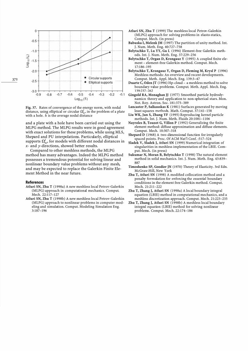
8/6/2019 A Critical Assessment of the Truly Meshless Local Petrov-Galerkin (MLPG),
http://slidepdf.com/reader/full/a-critical-assessment-of-the-truly-meshless-local-petrov-galerkin-mlpg 25/25
and a plate with a hole have been carried out using theMLPG method. The MLPG results were in good agreementwith exact solutions for these problems, while using MLS,Shepard and PU interpolations. Particularly, ellipticalsupports X I
te, for models with different nodal distances inx- and y-directions, showed better results.
Compared to other meshless methods, the MLPGmethod has many advantages. Indeed the MLPG methodpossesses a tremendous potential for solving linear andnonlinear boundary value problems without any mesh,and may be expected to replace the Galerkin Finite Ele-ment Method in the near future.
ReferencesAtluri SN, Zhu T (1998a) A new meshless local Petrov-Galerkin(MLPG) approach in computational mechanics. Comput.Mech. 22:117±127
Atluri SN, Zhu T (1998b) A new meshless local Petrov-Galerkin(MLPG) approach to nonlinear problems in computer mod-eling and simulation. Comput. Modeling Simulation Eng.3:187±196
Atluri SN, Zhu T (1999) The meshless local Petrov-Galerkin(MLPG) approach for solving problems in elasto-statics,Comput. Mech. (in press)
Babuska I, Melenk JM (1997) The partition of unity method. Int.J. Num. Meth. Eng. 40:727±758
Belytschko T, Lu YY, Gu L (1994) Element-free Galerkin meth-ods. Int. J. Num. Meth. Eng. 37:229±256
Belytschko T, Organ D, Krongauz Y (1995) A coupled ®nite ele-ment ± element-free Galerkin method. Comput. Mech.17:186±195
Belytschko T, Krongauz Y, Organ D, Fleming M, Krysl P (1996)Meshless methods: An overview and recent developments.Comput. Meth. Appl. Mech. Eng. 139:3±47
Duarte C, Oden JT (1996) Hp-cloud ± a meshless method to solveboundary-value problems. Comput. Meth. Appl. Mech. Eng.139:237±262
Gingold RA, Monaghan JJ (1977) Smoothed particle hydrody-namics: theory and application to non-spherical stars. Mon.Not. Roy. Astron. Soc. 181:375±389
Lancaster P, Salkauskas K (1981) Surfaces generated by movingleast squares methods. Math. Comput. 37:141±158
Liu WK, Jun S, Zhang YF (1995) Reproducing kernel particlemethods. Int. J. Num. Meth. Fluids 20:1081±1106
Nayroles B, Touzot G, Villon P (1992) Generalizing the ®niteelement method: diffuse approximation and diffuse elements.Comput. Mech. 10:307±318
Shepard D (1968) A two-dimensional function for irregularly spaced points. Proc. Of ACM Nat'l Conf. :517±524
Sladek V, Sladek J, Atluri SN (1999) Numerical integration of singularities in meshless implementation of the LBIE. Com-put. Mech. (in press)
Sukumar N, Moran B, Belytschko T (1998) The natural elementmethod in solid mechanics. Int. J. Num. Meth. Eng. 43:839±887
Timoshenko SP, Goodier JN (1970) Theory of Elasticity. 3rd Edn.McGraw-Hill, New York
Zhu T, Atluri SN (1998) A modi®ed collocation method and apenalty formulation for enforcing the essential boundary
conditions in the element free Galerkin method. Comput.Mech. 21:211±222Zhu T, Zhang J, Atluri SN (1998a) A local boundary integral
equation (LBIE) method in computational mechanics, and ameshless discretization approach. Comput. Mech. 21:223±235
Zhu T, Zhang J, Atluri SN (1998b) A meshless local boundary integral equation (LBIE) method for solving nonlinearproblems. Comput. Mech. 22:174±186
L o g
( r )
1 0
e
0
-0.5
-1.0
-1.5
-2.0
-2.5
-3.0-0.9 -0.8 -0.7 -0.6 -0.5 -0.4 -0.3 -0.2 -0.1
Log ( h _
)10
Circular supportsElliptical supports
Fig. 37. Rates of convergence of the energy norm, with nodaldistance, using elliptical or circular X J
tr , in the problem of a platewith a hole. "h is the average nodal distance
372