a course in quantum information theory

A Course in Quantum Information Theory

Ofer Shayevitz

Spring 2007

Based on lectures given at the Tel Aviv University

Edited by Anatoly Khina

Version compiled January 9, 2010

Contents

1 Preliminaries 3

I A Very Brief Introduction . . . . . . . . . . . . . . . . . . . . . . . . . . . . . . 3

I.1 Quantum Information Theory . . . . . . . . . . . . . . . . . . . . . . . . 3

I.2 Quantum Computing . . . . . . . . . . . . . . . . . . . . . . . . . . . . . 4

II Preliminaries: Linear Algebra . . . . . . . . . . . . . . . . . . . . . . . . . . . . 5

II.1 Notations . . . . . . . . . . . . . . . . . . . . . . . . . . . . . . . . . . . 5

II.2 Definitions and Basic Properties . . . . . . . . . . . . . . . . . . . . . . . 5

II.3 The Trace Operator . . . . . . . . . . . . . . . . . . . . . . . . . . . . . 7

III Postulates of Quantum Theory . . . . . . . . . . . . . . . . . . . . . . . . . . . 8

III.1 The State Space . . . . . . . . . . . . . . . . . . . . . . . . . . . . . . . . 8

III.2 Composite Systems and the Tensor Product . . . . . . . . . . . . . . . . 10

III.3 Unitary Evolution . . . . . . . . . . . . . . . . . . . . . . . . . . . . . . . 12

III.4 Measurements . . . . . . . . . . . . . . . . . . . . . . . . . . . . . . . . . 16

2 Basic Communication Protocols and Mixed States 23

I Superdense Coding . . . . . . . . . . . . . . . . . . . . . . . . . . . . . . . . . . 23

II Quantum Teleportation . . . . . . . . . . . . . . . . . . . . . . . . . . . . . . . . 24

III No Cloning . . . . . . . . . . . . . . . . . . . . . . . . . . . . . . . . . . . . . . 26

IV Mixed States Density Matrix . . . . . . . . . . . . . . . . . . . . . . . . . . . . . 27

V The Reduced Density Matrix . . . . . . . . . . . . . . . . . . . . . . . . . . . . 30

VI Remote State Preparation . . . . . . . . . . . . . . . . . . . . . . . . . . . . . . 33

VII The EPR Paradox and Bell Inequalities . . . . . . . . . . . . . . . . . . . . . . . 34

i

3 Quantum Compression 39

I The Quantum Compression Problem . . . . . . . . . . . . . . . . . . . . . . . . 39

I.1 Fidelity . . . . . . . . . . . . . . . . . . . . . . . . . . . . . . . . . . . . 39

I.2 Quantum Coding Scheme . . . . . . . . . . . . . . . . . . . . . . . . . . 40

I.3 AEP - Asymptotic Equipartition Property . . . . . . . . . . . . . . . . . 43

4 Quantum AEP and Von-Neumann Entropy Properties (Part I) 51

I Quantum Asymptotic Equipartition Property . . . . . . . . . . . . . . . . . . . 51

II Purification and Schmidt Decomposition . . . . . . . . . . . . . . . . . . . . . . 52

II.1 Purification . . . . . . . . . . . . . . . . . . . . . . . . . . . . . . . . . . 52

II.2 Schmidt Decomposition . . . . . . . . . . . . . . . . . . . . . . . . . . . 53

III Fidelity between Mixed States . . . . . . . . . . . . . . . . . . . . . . . . . . . . 55

IV Quantum Source Coding of an Ensemble of Mixed States . . . . . . . . . . . . . 56

V Information Quantities and Properties . . . . . . . . . . . . . . . . . . . . . . . 57

V.1 Von-Neumann Entropy Properties . . . . . . . . . . . . . . . . . . . . . . 59

5 Von-Neumann Entropy Properties

(Part II) 63

I Further Properties of the Von-Neumann Entropy . . . . . . . . . . . . . . . . . 63

II Accessible information . . . . . . . . . . . . . . . . . . . . . . . . . . . . . . . . 67

III The pretty good measurement (PGM) . . . . . . . . . . . . . . . . . . . . . . . 71

6 Quantum Channels and Classical Capacity 73

I Quantum Channels . . . . . . . . . . . . . . . . . . . . . . . . . . . . . . . . . . 73

I.1 Classical Capacity of a Quantum Channel . . . . . . . . . . . . . . . . . 75

7 Entanglement-Assisted Capacity and Entanglement Quantification 83

I Entanglement-Assisted Capacity . . . . . . . . . . . . . . . . . . . . . . . . . . . 83

I.1 Relation between CE and CCQ . . . . . . . . . . . . . . . . . . . . . . . . 89

II Quantifying Entanglement . . . . . . . . . . . . . . . . . . . . . . . . . . . . . . 89

ii

8 Further Notions of Capacity 93

I Operator-Sum Representation . . . . . . . . . . . . . . . . . . . . . . . . . . . . 93

II Entanglement Fidelity . . . . . . . . . . . . . . . . . . . . . . . . . . . . . . . . 95

III Coherent Communication . . . . . . . . . . . . . . . . . . . . . . . . . . . . . . 97

III.1 Replacing Classical Operations by Coherent Opeartions . . . . . . . . . . 98

IV Private / Secret-Key Classical Capacity . . . . . . . . . . . . . . . . . . . . . . . 99

V Entanglement-Generating Capacity . . . . . . . . . . . . . . . . . . . . . . . . . 103

VI The Quantum Channel Capacity . . . . . . . . . . . . . . . . . . . . . . . . . . 105

VI.1 Classically Assisted Quantum Capacity . . . . . . . . . . . . . . . . . . . 108

1

Chapter 1

Preliminaries

Summary by Y uval Regev.

I A Very Brief Introduction

I.1 Quantum Information Theory

Quantum information theory combines two distinct theories – (classical) information theory

and quantum mechanics. One might wonder, what does a theory of information have to do

with a physical theory? In classical information theory we are usually not very concerned with

this relation, as the theory is abstract enough and does not depend on any specific physical

media. However, information is still a physical quantity, as it is stored, measured, transmitted

and received using physical devices. The most basic element of classical information theory is

the (classical) bit. A bit is represented in practice by some classical physical quantity such

as voltage or magnetization, and the statistical laws governing the way it can be processed

are derived from the relevant (classical) physical theory. In the information theoretic regime,

these statistical laws are all that is required in order to determine the fundamental limits of

information processing.

The basic element in quantum information theory is the quantum bit, or qubit. Similarly to a

classical bit, the qubit is a physical quantity. In contrast however, it obeys the laws of quantum

mechanics. As we shall see, information under the laws of quantum mechanics behaves in a

markedly different way than classical information, which cannot be captured using the classical

tools. One example is the renowned no cloning Theorem, which states that (unlike a bit) a qubit

cannot be accurately duplicated. The following example demonstrates an even more peculiar

aspect of that behavior. We will return to this example at the end of the course.

3

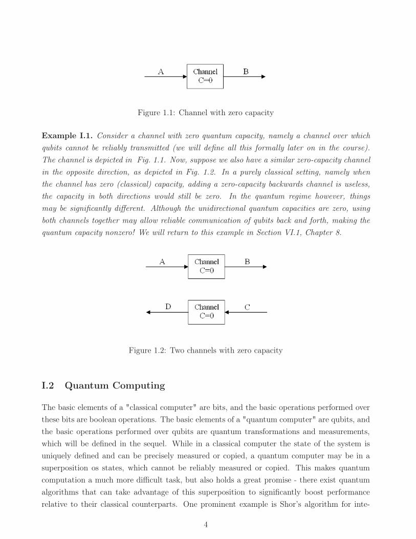
Figure 1.1: Channel with zero capacity

Example I.1. Consider a channel with zero quantum capacity, namely a channel over which

qubits cannot be reliably transmitted (we will define all this formally later on in the course).

The channel is depicted in Fig. 1.1. Now, suppose we also have a similar zero-capacity channel

in the opposite direction, as depicted in Fig. 1.2. In a purely classical setting, namely when

the channel has zero (classical) capacity, adding a zero-capacity backwards channel is useless,

the capacity in both directions would still be zero. In the quantum regime however, things

may be significantly different. Although the unidirectional quantum capacities are zero, using

both channels together may allow reliable communication of qubits back and forth, making the

quantum capacity nonzero! We will return to this example in Section VI.1, Chapter 8.

Figure 1.2: Two channels with zero capacity

I.2 Quantum Computing

The basic elements of a "classical computer" are bits, and the basic operations performed over

these bits are boolean operations. The basic elements of a "quantum computer" are qubits, and

the basic operations performed over qubits are quantum transformations and measurements,

which will be defined in the sequel. While in a classical computer the state of the system is

uniquely defined and can be precisely measured or copied, a quantum computer may be in a

superposition os states, which cannot be reliably measured or copied. This makes quantum

computation a much more difficult task, but also holds a great promise - there exist quantum

algorithms that can take advantage of this superposition to significantly boost performance

relative to their classical counterparts. One prominent example is Shor’s algorithm for inte-

4

ger factorization which runs in polynomial time on a quantum computer, in contrast to the

exponential complexity of the best known classical algorithms.

II Preliminaries: Linear Algebra

II.1 Notations

• Hn - Hilbert space of dimension n (a.k.a “inner product space”).

• |ψ〉 - ket - vector in Hn (column vector when representing Hn w.r.t. an orthonormal

base).

• 〈ψ| - bra - conjugate transpose of |ψ〉.

• 〈ψ|φ〉 - braket - inner product between |ψ〉 and |φ〉.

Property II.1 (Inner Product Properties). 1. Conjugate Symmetry: 〈ψ|φ〉 = 〈φ|ψ〉∗.

2. Linearity in the second vector: 〈φ| (a|ψ1〉 + b|ψ2〉) = a〈ψ|φ1〉 + b〈ψ|φ2〉.

3. Non-negativity: 〈ψ|ψ〉 ≥ 0, 〈ψ|ψ〉 = 0 ⇔ |ψ〉 = 0.

II.2 Definitions and Basic Properties

Definition II.1 (Linear Operator). A linear operator can always be represented by a corre-

sponding matrix with respect to some orthonormal space. We shall use operators and their

corresponding matrices interchangeably.

Definition II.2 (Adjoint Opeartor). The operator A† is the adjoint operator of A, if it satisfies

〈ψ|A†|φ〉 = 〈φ|A|ψ〉∗ for every φ, ψ ∈ H. If we represent the operator A by a matrix according

to some orthonormal base, then the conjugate transpose of this matrix is the representation

matrix of A†.

Definition II.3 (Outer Product). The outer product between |ψ〉 and |φ〉 is the operator:

|ψ〉〈φ|. 〈φ| is an operator from Hn to C(projects onto the state |φ〉), and |ψ〉 is an operator

from C to Hn.

Example II.1. (|w〉〈v|) (|u〉) = |w〉〈v|u〉︸︷︷︸scalar

= 〈v|u〉|w〉.

Lemma II.1. If |i〉ni=1 is an orthonormal basis of Hn then∑n

i=1 |i〉〈i| = I.

5

Proof. Let v be any vector in H. Then, it has a unique representation according to the or-

thonormal basis |i〉ni=1,∑

j αj |j〉. Hence

(∑

i

|i〉〈i|)|v〉 =

(∑

i

|i〉〈i|)(

∑

j

αj|j〉)

=∑

i,j

αj |i〉〈i|j〉︸︷︷︸δij

=∑

j

αj |j〉 = |v〉.

Lemma II.2. If |i〉ki=1 is an orthonormal basis of the sub-space Gk of the Hilbert space Hn

(k ≤ n), then the operator P =∑k

i |i〉〈i| is a projection operator onto Gk. Namely, the following

properties hold:

Property II.2 (Projector).

(i) P = P †.

(ii) P = P 2.

Remark II.1. Note that I − P is a projector onto the orthogonal subspace G⊥k .

Lemma II.3 (Spectral Decomposition). Let A be a Hermitian matrix, namely A = A†. Then A

can be unitarily diagonalized , i.e., there exists an orthonormal basis composed of its eigenvectors

|i〉ni=1 of A, such that

A =

n∑

i=1

λi|i〉〈i|,

where λini=1 are the corresponding (real) eigenvalues.

Thus, a Hermitian operator can always be represented by some linear combination of projection

operators.

Definition II.4 (Positive Opeartor). An operator A is Positive (resp. Positive Definite) if all

of its eigenvalues λi are real and non-negative (resp. positive), or equivalently if 〈ψ|A|ψ〉 ≥ 0

(resp. > 0) for all |ψ〉 (resp. |ψ〉 6= 0).

Note that a Positive operator (matrix) over Hn is necessarily Hermitian (this statement is not

true over Rn, namely not any Positive operator (matrix) is Symmetric).

Lemma II.4. The matrix A†A is positive for every A.

6

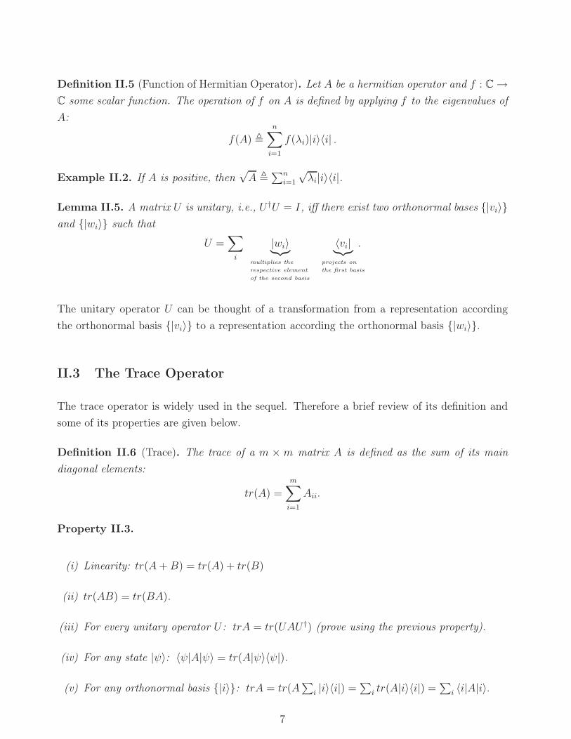
Definition II.5 (Function of Hermitian Operator). Let A be a hermitian operator and f : C →C some scalar function. The operation of f on A is defined by applying f to the eigenvalues of

A:

f(A) ,

n∑

i=1

f(λi)|i〉〈i| .

Example II.2. If A is positive, then√A ,

∑ni=1

√λi|i〉〈i|.

Lemma II.5. A matrix U is unitary, i.e., U †U = I, iff there exist two orthonormal bases |vi〉and |wi〉 such that

U =∑

i

|wi〉︸︷︷︸multiplies the

respective element

of the second basis

〈vi|︸︷︷︸projects on

the first basis

.

The unitary operator U can be thought of a transformation from a representation according

the orthonormal basis |vi〉 to a representation according the orthonormal basis |wi〉.

II.3 The Trace Operator

The trace operator is widely used in the sequel. Therefore a brief review of its definition and

some of its properties are given below.

Definition II.6 (Trace). The trace of a m × m matrix A is defined as the sum of its main

diagonal elements:

tr(A) =

m∑

i=1

Aii.

Property II.3.

(i) Linearity: tr(A+B) = tr(A) + tr(B)

(ii) tr(AB) = tr(BA).

(iii) For every unitary operator U : trA = tr(UAU †) (prove using the previous property).

(iv) For any state |ψ〉: 〈ψ|A|ψ〉 = tr(A|ψ〉〈ψ|).

(v) For any orthonormal basis |i〉: trA = tr(A∑

i |i〉〈i|) =∑

i tr(A|i〉〈i|) =∑

i 〈i|A|i〉.

7

III Postulates of Quantum Theory

III.1 The State Space

Postulate I. A closed physical system is described by a state vector, which is a unit vector

in a Hilbert Space called the state space of the physical system.

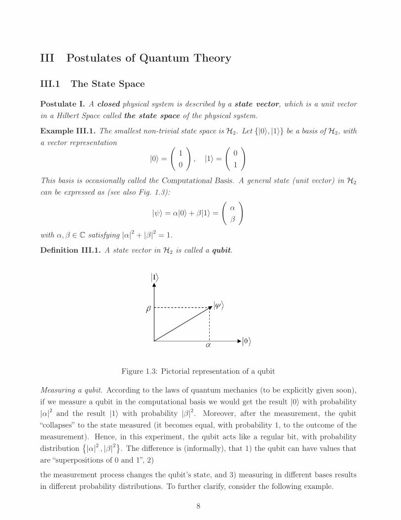
Example III.1. The smallest non-trivial state space is H2. Let |0〉, |1〉 be a basis of H2, with

a vector representation

|0〉 =

(1

0

), |1〉 =

(0

1

)

This basis is occasionally called the Computational Basis. A general state (unit vector) in H2

can be expressed as (see also Fig. 1.3):

|ψ〉 = α|0〉 + β|1〉 =

(α

β

)

with α, β ∈ C satisfying |α|2 + |β|2 = 1.

Definition III.1. A state vector in H2 is called a qubit.

Figure 1.3: Pictorial representation of a qubit

Measuring a qubit. According to the laws of quantum mechanics (to be explicitly given soon),

if we measure a qubit in the computational basis we would get the result |0〉 with probability

|α|2 and the result |1〉 with probability |β|2. Moreover, after the measurement, the qubit

“collapses” to the state measured (it becomes equal, with probability 1, to the outcome of the

measurement). Hence, in this experiment, the qubit acts like a regular bit, with probability

distribution|α|2 , |β|2

. The difference is (informally), that 1) the qubit can have values that

are “superpositions of 0 and 1”, 2)

the measurement process changes the qubit’s state, and 3) measuring in different bases results

in different probability distributions. To further clarify, consider the following example.

8

Example III.2 (Measuring in different bases). Define the two (orthonormal) states in H2:

|+〉 = 1√2(|0〉 + |1〉) ,

|−〉 = 1√2(|0〉 − |1〉) .

These states can be written in a vector notations as (see also Fig. 1.4):

|0〉 =

(1

0

), |1〉 =

(0

1

), |+〉 =

1√2

(1

1

), |−〉 =

1√2

(1

−1

).

Figure 1.4: Pictorial representation of |0〉, |1〉, |+〉 and |−〉

Suppose that the initial state of the system is |+〉, and a measurement is performed. The

measurement can be made is different bases:

1. Measurment in the computational base: We get one of the results 0, 1 with equal

probability. The system collapses to one of the states |0〉, |1〉, depends on the result of

the measurment.

2. Measurment in the basis |+〉, |−〉: We get the result + with probability 1. The state

does not change.

3. Measurment in the basis |+〉, |−〉 after measuring in the computational base:

We get one of the resutls +,− with equal probability. After the first measurement

(in the computational base) the qubit collapsed to either |0〉 or |1〉, and after the second

measurement (the one in |+〉, |−〉 we get +,− with equal probabilities.

Thus the act of measuring itself, effects the state of the system. We will elaborate on the

measurement process when we get to Postulate IV.

9

III.2 Composite Systems and the Tensor Product

Let us continue our informal introduction, and discuss a system of more than one qubit.

Example III.3 (Two qubit system). As we have seen before, one qubit is a normalized vector

in a two-dimensional space (with analogy to the classical bit, which can take one of two possible

values). Following this logic, two qubits are defined as a normalized vector in a four-dimensional

space (two classical bits correspond to four distinct values).

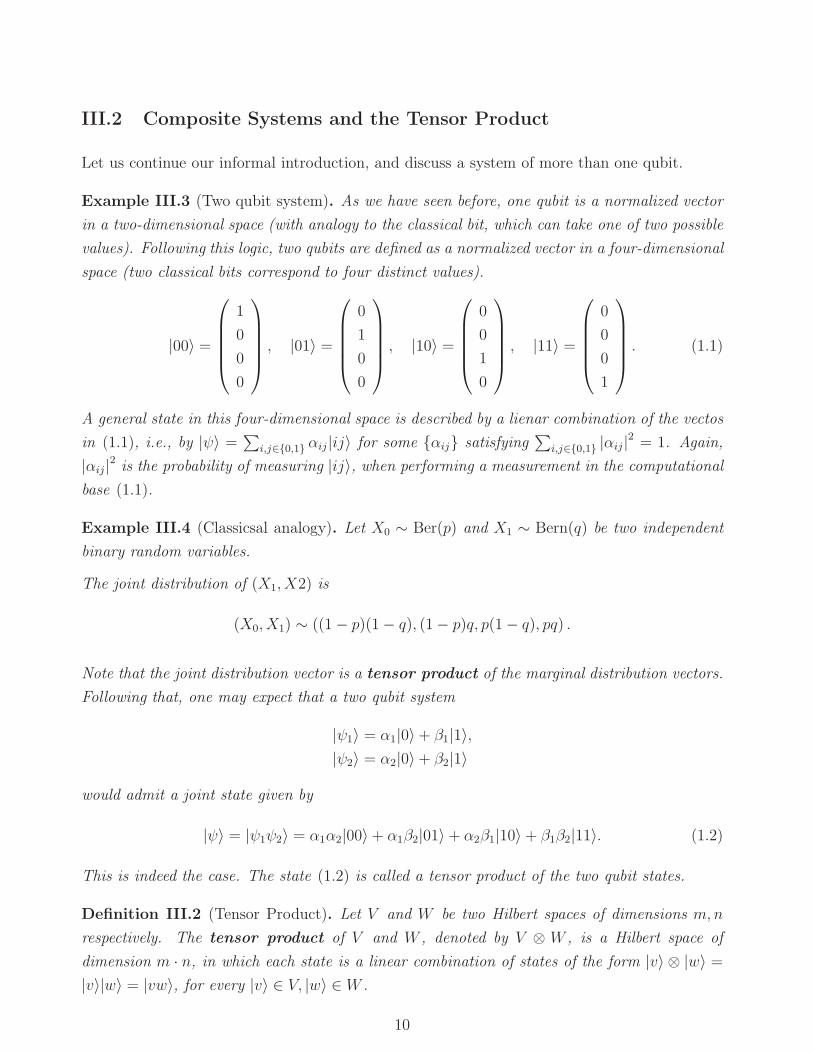
|00〉 =

1

0

0

0

, |01〉 =

0

1

0

0

, |10〉 =

0

0

1

0

, |11〉 =

0

0

0

1

. (1.1)

A general state in this four-dimensional space is described by a lienar combination of the vectos

in (1.1), i.e., by |ψ〉 =∑

i,j∈0,1 αij |ij〉 for some αij satisfying∑

i,j∈0,1 |αij |2 = 1. Again,

|αij|2 is the probability of measuring |ij〉, when performing a measurement in the computational

base (1.1).

Example III.4 (Classicsal analogy). Let X0 ∼ Ber(p) and X1 ∼ Bern(q) be two independent

binary random variables.

The joint distribution of (X1, X2) is

(X0, X1) ∼ ((1 − p)(1 − q), (1 − p)q, p(1 − q), pq) .

Note that the joint distribution vector is a tensor product of the marginal distribution vectors.

Following that, one may expect that a two qubit system

|ψ1〉 = α1|0〉 + β1|1〉,|ψ2〉 = α2|0〉 + β2|1〉

would admit a joint state given by

|ψ〉 = |ψ1ψ2〉 = α1α2|00〉 + α1β2|01〉 + α2β1|10〉 + β1β2|11〉. (1.2)

This is indeed the case. The state (1.2) is called a tensor product of the two qubit states.

Definition III.2 (Tensor Product). Let V and W be two Hilbert spaces of dimensions m,n

respectively. The tensor product of V and W , denoted by V ⊗ W , is a Hilbert space of

dimension m · n, in which each state is a linear combination of states of the form |v〉 ⊗ |w〉 =

|v〉|w〉 = |vw〉, for every |v〉 ∈ V, |w〉 ∈W .

10

The natural inner product in the space V ⊗W (induced by the inner products of the spaces V

and W ) is: (∑

i

ai|viwi〉 ,∑

j

bj |v′

jw′

j〉)

,∑

i,j

a∗i bj〈vi|v′

j〉〈wi|w′

j〉.

Property III.1 (Properties of tensor product).

1. Linearity in both variables.

2. Let |i〉ni=1 and |j〉mj=1 be two orthonormal bases of the space V and W , respectively.

Then |ij〉 is an orthonormal bas of the space V ⊗W .

Example III.5 (Tensor product of H2 spaces). Let V = W = H2 and consider the respective

states|ψv〉 = 1√

2(|0〉 + |1〉)

|ψw〉 = 1√2(|0〉 − |1〉) .

Using Property III.1 we have:

|ψvψw〉 =1

2(|0〉 + |1〉) (|0〉 − |1〉) =

1

2(|00〉 + |10〉 − |01〉 − |11〉) ,

where |ψvψw〉 ∈ V ⊗W . Had we chosen the orthonormal basis |+〉, |−〉 for W , we would

have gotten:

|ψvψw〉 =1√2

(|0−〉 + |1−〉) = | + −〉 .

Example III.6 (Inner product in tensor product space). Continuing the previous example, we

define two states in the tensor product space V ⊗W :

|ψ1〉 = 1√2(|00〉 + |11〉) (EPR state)

|ψ2〉 = 1√2(|0〉 + |1〉) |0〉 = 1√

2(|00〉 + |10〉) .

The inner product of these two states is:

〈ψ1|ψ2〉 =1

2(〈00|00〉+ 〈00|10〉 + 〈11|00〉+ 〈11|10〉) (1.3)

=1

2

〈0|0〉︸︷︷︸

1

〈0|0〉︸︷︷︸1

+ 〈0|1〉︸︷︷︸0

〈0|0〉︸︷︷︸1

+ 〈1|0〉︸︷︷︸0

〈1|0〉︸︷︷︸0

+ 〈1|1〉︸︷︷︸1

〈1|0〉︸︷︷︸0

=1

2.

where first equality follows from Property III.1. An alternative way of deriving the same result,

is recalling that (1.1) forms an orthonormal basis in H4, and therefore only the term 〈00|00〉,in (1.3) differs from 0.

11

We are now ready for the next postulate.

Postulate II. The state space of a “composite” system (a system which is composed of several

sub-systems) is the tensor product of the state spaces of the sub-systems. Furthermore, if the

k-th (1 ≤ k ≤ n) sub-system is in state |ψk〉, then the composite system is in state |ψ〉 =

|ψ1〉 ⊗ |ψ2〉 ⊗ · · · ⊗ |ψn〉.

Remark III.1. The converse is not necessarily true: not every state of the composite system

can be decomposed into a tensor product of states of the sub-systems composing it.

Remark III.1 leads us to the notion of entanglement.

Entanglement

Definition III.3 (Entangled state). A state of a composite system, which cannot be written as

a tensor product of states of the sub-systems composing it, is said to be entangled. The two

sub-systems are also called entangled.

Example III.7 (EPR state). The state |ψ〉 = 1√2(|00〉 + |11〉) (one of the EPR states) cannot

be decomposed into the form |ψ〉 = |a〉|b〉, and thus is entangled.

In an entangled state, it is not possible to define the state of each of the sub-systems. Each sub-

system is found in a state which is a combination of several states, with a certain probability

distribution.

III.3 Unitary Evolution

Postulate III. The evolution of a closed quantum system is described by a unitary operator

(unitary transformation). Namely, if |ψ1〉 and |ψ2〉 are the states of the system in times t1 and

t2, then

|ψ2〉 = U |ψ1〉,

where U is unitary and depends only on t1 and t2.

Remark III.2.

(i) The transformation must be unitary in order to preserve the norm - the resulting state

must be of unit length at all times.

(ii) The evolution of a closed physical system is reversible - it is possible to go from state |ψ2〉to state |ψ1〉 by applying the inverse operator U−1 = U †.

12

Example III.8 (Pauli matrices).

• Quantum NOT (bit flip): |0〉 −→ |1〉, |1〉 −→ |0〉

X =

(0 1

1 0

), XX† = I

X (α|0〉 + β|1〉) = X

(α

β

)=

(β

α

)= β|0〉 + α|1〉

• Phase flip: |0〉 −→ |0〉, |1〉 −→ −|1〉

Z =

(1 0

0 −1

), ZZ† = I

• |0〉 −→ i|1〉, |1〉 −→ −i|0〉

Y =

(0 −ii 0

), Y Y † = I

The matrices I,X, Y, Z are called Pauli Matrices, and they form a basis of the complex

2 × 2 matrix space.

Definition III.4 (Hadamard matrix).

H =1√2

(1 1

1 −1

)

The Hadamard matrix transforms the states |0〉, |1〉 to the states |+〉, |−〉:

H|0〉 =1√2

(|0〉 + |1〉) = |+〉

H|1〉 =1√2

(|0〉 − |1〉) = |−〉 .

Example III.9 (Quantum operations on two qubits).

• Controlled-NOT (CNOT) Gate: The CNOT gate (operator) is described by the fol-

lowing unitary matrix (see Fig. 1.5 for a schematic representation):

1 0

0 10

00 1

1 0

=

(I 0

0 X

)

13

The operation of the CNOT gate in the computational basis is given by

|00〉 −→ |00〉 ,|01〉 −→ |01〉 ,|10〉 −→ |11〉 ,|11〉 −→ |10〉 .

Or using dirac notations, |ij〉 CNOT−→ |i〉|i⊕ j〉. The second qubit is flipped if the first qubit

is 1.

Figure 1.5: Schematic representation of a CNOT gate

• Controlled-U Gate: Similarly to the CNOT gate, the first qubit controls whether the U

operation will be performed on the remaining qubits (see also Fig. 1.6).

(I 0

0 U

)

Figure 1.6: Schematic representation of a controlled-U gate

Definition III.5. Local operations are operation which are applied to only a sub-system,

whereas the remaining sub-systems remain untouched.

Example III.10 (Local operations). Fig. 1.7) schematically depicts an operation X applied to

the first qubit, and H to the second qubit. This has the following meaning:

14

Figure 1.7: X applied to the first qubit and H to the second one

|00〉 X1→ |10〉 H2→ |1+〉 = |1〉 · 1√2(|0〉 + |1〉) = 1√

2(|10〉 + |11〉)

|01〉 X1→ |11〉 H2→ |1−〉 = 1√2(|10〉 − |11〉)

|10〉 X1→ |00〉 H2→ |0+〉 = 1√2(|00〉 + |01〉)

|11〉 X1→ |01〉 H2→ |0−〉 = 1√2(|00〉 − |01〉) ,

where, in general, Gi means applying with the operator G on the ith qubit. The matrix describing

the operation on the whole system is:

1√2

0 0

0 0

1 1

1 −1

1 1

1 −1

0 0

0 0

= X ⊗H ,

where in the last equality we used the following definition.

Definition III.6 (Matrix tensor product). The tensor product between matrix A ∈ Cm×n and

matrix B ∈ Cp×q is a matrix of size pm× qn, which has the form:

A⊗B =

a11B a12B · · · a1nB

a21B. . .

......

. . ....

am1B · · · · · · amnB

.

Assertion III.1. After applying a tensor product of two operators U ⊗V on a composite state

|ψ1ψ2〉, the resulting state is the tensor product of the sub-states after applying the local operators

to them:

|ψ1ψ2〉 U1V2−→ (U ⊗ V ) |ψ1ψ2〉 = (U |ψ1〉) (V |ψ2〉)

15

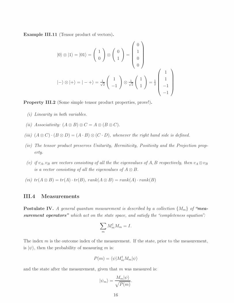
Example III.11 (Tensor product of vectors).

|0〉 ⊗ |1〉 = |01〉 =

(1

0

)⊗(

0

1

)=

0

1

0

0

|−〉 ⊗ |+〉 = | − +〉 = 1√2

(1

−1

)⊗ 1√

2

(1

1

)= 1

2

1

1

−1

−1

Property III.2 (Some simple tensor product properties, prove!).

(i) Linearity in both variables.

(ii) Associativity: (A⊗ B) ⊗ C = A⊗ (B ⊗ C).

(iii) (A⊗ C) · (B ⊗D) = (A ·B) ⊗ (C ·D), whenever the right hand side is defined.

(iv) The tensor product preserves Unitarity, Hermiticity, Positivity and the Projection prop-

erty.

(v) if vA, vB are vectors consisting of all the the eigenvalues of A,B respectively, then vA⊗vBis a vector consisting of all the eigenvalues of A⊗B.

(vi) tr(A⊗ B) = tr(A) · tr(B), rank(A⊗ B) = rank(A) · rank(B)

III.4 Measurements

Postulate IV. A general quantum measurement is described by a collection Mm of “mea-

surement operators” which act on the state space, and satisfy the “completeness equation”:

∑

m

M †mMm = I.

The index m is the outcome index of the measurement. If the state, prior to the measurement,

is |ψ〉, then the probability of measuring m is:

P (m) = 〈ψ|M †mMm|ψ〉

and the state after the measurement, given that m was measured is:

|ψm〉 =Mm|ψ〉√P (m)

.

16

Note that the “completeness equation” is equivalent to the requirement that the sum of all

probabilities is equal to 1:

∑

m

P (m) =∑

m

〈ψ|M †mMm|ψ〉 = 〈ψ|(∑

m

M †mMm

)|ψ〉 = 1, ∀ψ ∈ H

.

Remark III.3. The number of measurement operators can be smaller, larger or equal to the

dimension of the state space.

Example III.12 (Measuring a qubit). To perform a measurement in the computational base,

the projectors on the axes are used:

M0 = |0〉〈0| ,M1 = |1〉〈1| .

Using the property of projection operators P 2 = P , one notes that these projectors satisfy the

completeness equation:

M †0M0 +M †1M1 = M20 +M2

1 = M0 +M1 = |0〉〈0| + |1〉〈1| = I .

Measuring the qubit |ψ〉 = α|0〉 + β|1〉, using the projectors above, we get the result 0 with

probability

P (0) = 〈ψ|M †0M0|ψ〉 = (α∗〈0| + β∗〈1|) |0〉〈0|︸︷︷︸M0

(α|0〉 + β|1〉) = α∗α = |α|2

and the result 1 with probability P (1) = |β|2. Given that the result of the measurement was 0

(for example), the state collapses to the new state

|ψ0〉 =M0|ψ〉√P (0)

=α|0〉|α| = ejθα|0〉 = |0〉 .

The last transition requires an explanation.

Remark III.4. The postulates can be modified such that a state vector is defined up to a global

phase, i.e., up to a multiplication by any ejθ. This does not change anything, since a global

phase has no influence on measurements or their outcomes/probabilities. Therefore, we can

always disregard a global phase.

In a similar manner, to perform a measure in the basis |+〉, |−〉, one needs to use the mea-

surement operators M0 = |+〉〈+|, M1 = |−〉〈−|. We can also perform the measurement by

first “rotating” the state using the operator H, measuring in the computational base, and then

“rotating” the state back using H† = H.

17

Example III.13 (Measuring one of two qubits). Let

|ψ〉 =∑

i,j∈0,1αij |ij〉

be the states of some composite system AB. We want to measure only the first qubit, in the

computational base. The measurement operators which achieve this are:

M0 = (|0〉〈0|) ⊗ I =

(1

0

)(1 0

)⊗(

1 0

0 1

)=

1 0

0 1

0 0

0 0

0 0

0 0

0 0

0 0

=

(I 0

0 0

)

M1 = (|1〉〈1|) ⊗ I = . . . =

(0 0

0 I

).

The probabilty of the possible outcomes are:

P (0) = 〈ψ|M0|ψ〉 = |α00|2 + |α01|2

P (1) = 〈ψ|M1|ψ〉 = |α10|2 + |α11|2.

After measuring the result 0, the state collapses to the state:

|ψ0〉 =α00|00〉 + α01|01〉√

|α00|2 + |α01|2=

1√|α00|2 + |α01|2

|0〉 (α00|0〉 + α01|1〉) .

Definition III.7 (POVM). “Positive Opeartor Valued Measure” (POVM) is a measurement

which is described by a set of positive operators Em which satisfy∑

mEm = I. The

probability of the result m is then P (m) = 〈ψ|Em|ψ〉.

Remark III.5. Definition III.7 is a special case of Postulate IV, taking Em = M †mMm. We

therefore use POVM when we care only about the probabilities of the measurement outcome,

and not about the state after the measurement. It is sometimes more convenient to work with.

The POVM used in Example III.12 is E0 = M †0M0 = M0 and E1 = M †1M1 = M1.

Definition III.8 (Orthogonal Projection Operators). Orthogonal projectors are a set of oper-

ators Pm, which satisfy: Pm = P †mPmPk = Pmδmk

Measurement performed using sets composed of only orthogonal projectors are called Von-

Neumann (VN) measurements.

Remark III.6. Orthogonal measurements are a special case of the general measurement oper-

ation, described in Postulate IV. Furthermore, in this case the POVM and the measurement

operators are exactly the same, as in Example III.12.

18

Definition III.9 (Observable). Von-Neumann measurement can be described by a hermitian

operator termed observable:

M =∑

m

m︸︷︷︸Measurement outcomes

= Eigenvalues of M

Pm︸︷︷︸Orthogonal

projectors

The exepcted value of the outcome of the measurement is:

< M > = E (M) =∑

m

mp(m)

=∑

m

m〈ψ|Pm|ψ〉 = |ψ〉(∑

m

mp(m)

)|ψ〉

= 〈ψ|M |ψ〉 = tr (M |ψ〉〈ψ|) , (1.4)

where tr stands for trace (see Section II.3, Chapter 2).

Example III.14.

• The observable Z =

(1 0

0 −1

)describes a measurement in the computational basis

|0〉, |1〉 with the measurement outcomes (eigenvalues) ±1.

• The observable X =

(0 1

1 0

)describes a measurement in the basis |+〉, |−〉 with

the measurement outcomes (eigenvalues) ±1. If we calculate the expected value of the

outcome, when measuring the state |0〉, we have

tr (X|0〉〈0|) = tr

((0 1

1 0

)(1 0

0 0

))= tr

((0 0

1 0

))= 0.

since we get |+〉 and |−〉 with equal probabilities.

Definition III.10 (Distinguishability). Two states are called seperable or distinguishable if

there exists a measurement that can distinguish between the two states with certainty (w.p. 1).

Example III.15. A qubit is in a state |ϕ〉 or |ψ〉, and 〈ϕ|ψ〉 6= 0. We already know these

states cannot be reliably distinguished. Suppose however we add an “erasure option”, namely

after measuring we can announce the state is |ϕ〉 or |ψ〉, but we can also announce we cannot

decide. Of course, we cannot use an orthogonal measurement to that end, as that will yield only

two results. Can we find another set of measurements that will give us a zero probability for a

wrong detection? Consider the POVM

E0 = a (I − |ϕ〉〈ϕ|)E1 = b (I − |ψ〉〈ψ|)E2 = I − E0 − E1

19

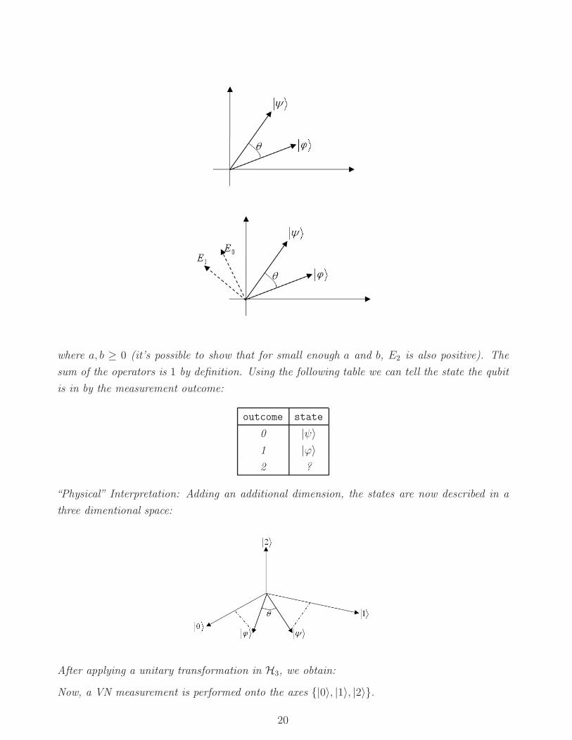
where a, b ≥ 0 (it’s possible to show that for small enough a and b, E2 is also positive). The

sum of the operators is 1 by definition. Using the following table we can tell the state the qubit

is in by the measurement outcome:

outcome state

0 |ψ〉1 |ϕ〉2 ?

“Physical” Interpretation: Adding an additional dimension, the states are now described in a

three dimentional space:

After applying a unitary transformation in H3, we obtain:

Now, a VN measurement is performed onto the axes |0〉, |1〉, |2〉.

20

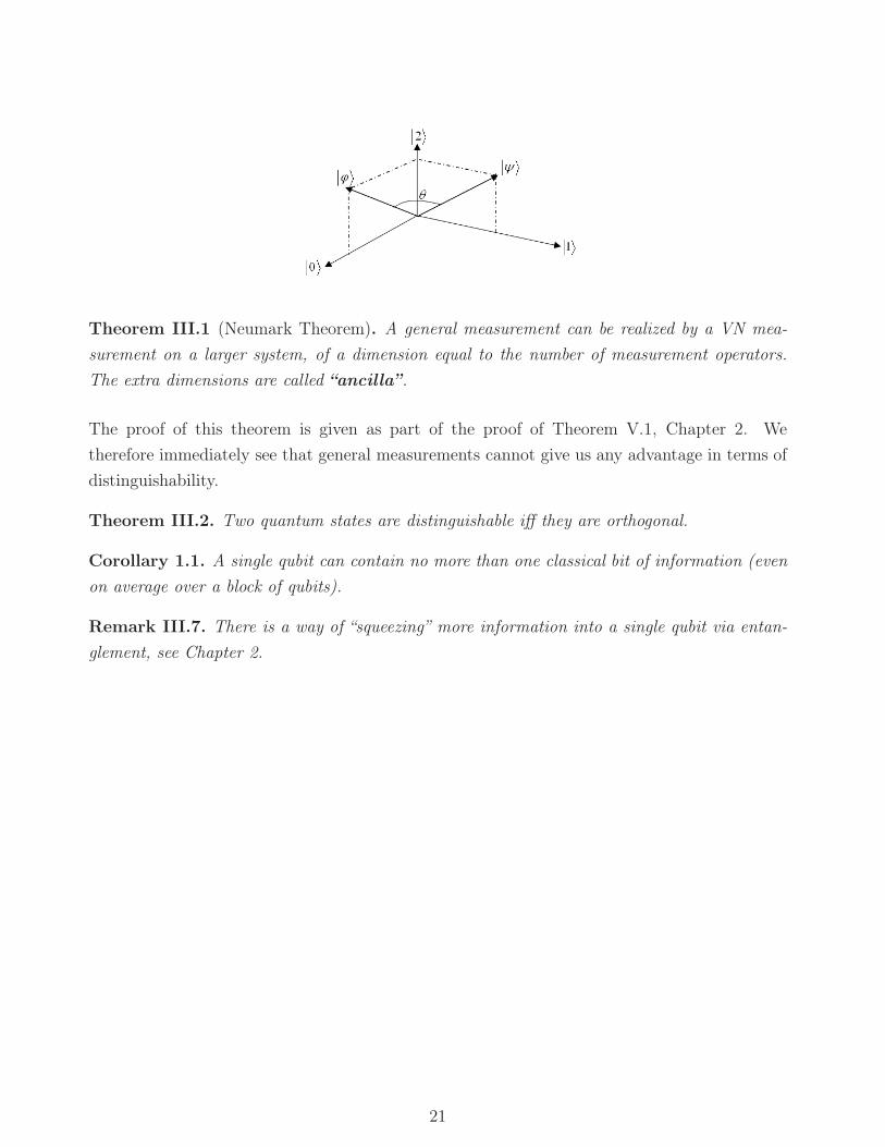
Theorem III.1 (Neumark Theorem). A general measurement can be realized by a VN mea-

surement on a larger system, of a dimension equal to the number of measurement operators.

The extra dimensions are called “ancilla”.

The proof of this theorem is given as part of the proof of Theorem V.1, Chapter 2. We

therefore immediately see that general measurements cannot give us any advantage in terms of

distinguishability.

Theorem III.2. Two quantum states are distinguishable iff they are orthogonal.

Corollary 1.1. A single qubit can contain no more than one classical bit of information (even

on average over a block of qubits).

Remark III.7. There is a way of “squeezing” more information into a single qubit via entan-

glement, see Chapter 2.

21

Chapter 2

Basic Communication Protocols and

Mixed States

Summary by Amir Ingber.

I Superdense Coding

Suppose Alice wished to transmit two (classical) bits to Bob by using only a single qubit. As was

claimed in Corollary 1.1, Chapter 1, this is not possible unless Alice and Bob share entangled

states. In superdense coding (SDC), we assume that Alice and Bob share one of the following

states:

|β00〉 =1√2(|00〉 + |11〉),

|β01〉 =1√2(|00〉 − |11〉),

|β10〉 =1√2(|01〉 + |10〉),

|β11〉 =1√2(|01〉 − |10〉).

commonly known as Bell or EPR states (Einstein, Podolsky and Rosen). One may easily verify

that these states form an orthonormal basis for H4 and that the two qubits, forming each of

these states, are entangled.

An important property of the Bell states is that each state is reachable from any other state

by a local operation (see Definition III.5, Chapter 1), in our case , a local operation in Alice’s

side only. For example, if we start at |β00〉:

23

|β00〉 I1−→ |β00〉,|β00〉 Z1−→ |β01〉,|β00〉 X1−→ |β10〉,|β00〉 X1Z1−→ |β11〉,

where the operations I, Z, and X, are the Pauli matrices defined in Example III.8, Chapter 1.

Algorithm I.1 (SDC). Alice activates one of the four operations on her qubit according to her

two classical bits. She then sends her qubit to Bob. Bob performs a measurement, using the

Bell basis, and reconstructs the bits with probability 1.

Remark I.1.

• We see clearly that entanglement is an information theoretic resource (reminds of classical

common randomness, only “stronger”).

• A Bell state is commonly called an entangled bit, or ebit. The resource relation stemming

from the SDC protocol is:

1qubit + 1ebit≥

=⇒ 2cbits. (2.1)

• It turns out that (2.1) is tight, namely no more than 2 classical bits can be conveyed using

a shared Bell state. If the qubits are not fully entangled, then the information that can be

conveyed (on average) is between 1 and 2 cbits.

• Information security: if the transmitted qubit falls into the hands of eavesdroppers they

can extract no information from it regarding the classical bits that Alice is trying to send:

it can be shown that the result of any measurement applied to this qubit is independent of

the cbits.

II Quantum Teleportation

We saw that entanglement can be used in order to convey more classical information via trans-

mission of qubits. We now show how entanglement allows the conveying of qubits using classical

transmission.

Consider the case where Alice wishes to transmit a qubit |ϕ〉 = α|0〉 + β|1〉, by sending only

classical information (bits) through a classical channel.

24

Hϕ

2mX 1mZ

00β

Alice

Bob

1m

2m

ϕ

0ϕ 1ϕ 2ϕ 3ϕ

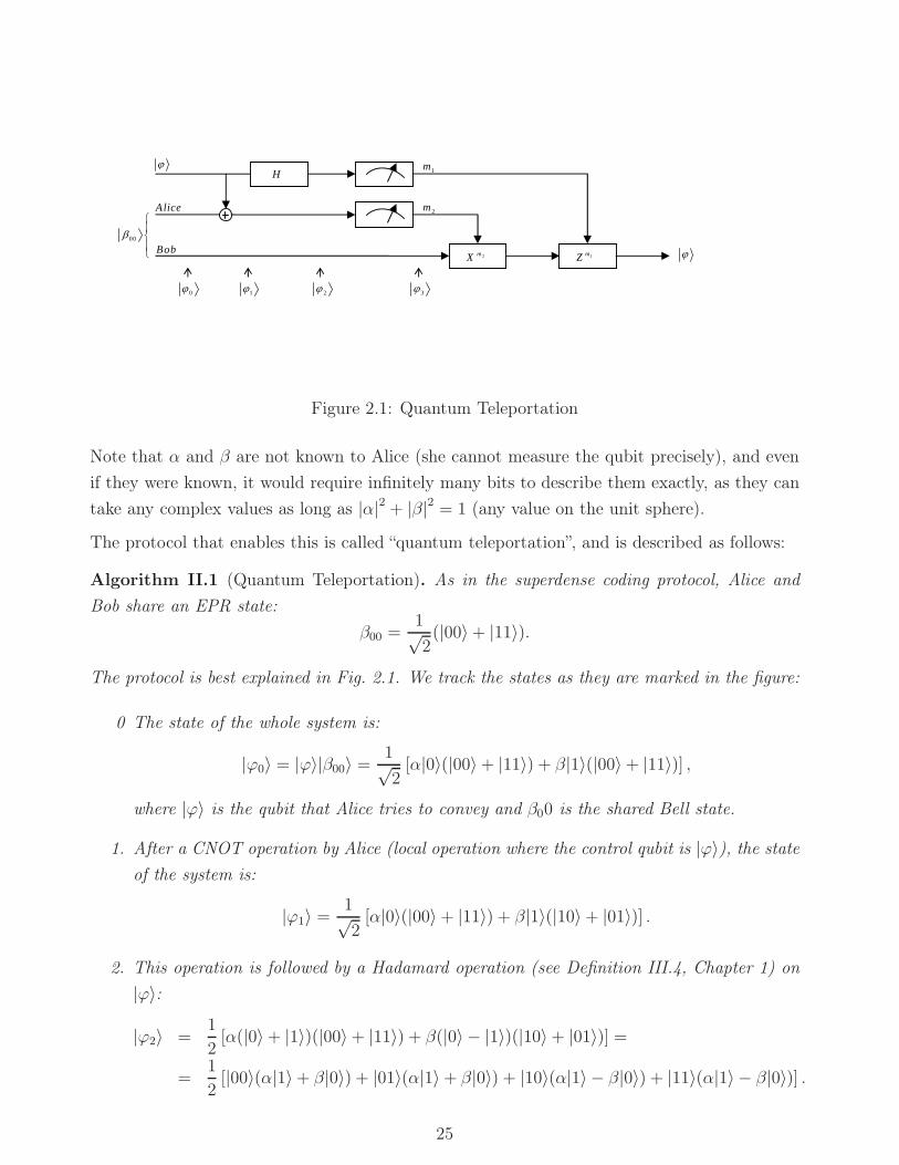
Figure 2.1: Quantum Teleportation

Note that α and β are not known to Alice (she cannot measure the qubit precisely), and even

if they were known, it would require infinitely many bits to describe them exactly, as they can

take any complex values as long as |α|2 + |β|2 = 1 (any value on the unit sphere).

The protocol that enables this is called “quantum teleportation”, and is described as follows:

Algorithm II.1 (Quantum Teleportation). As in the superdense coding protocol, Alice and

Bob share an EPR state:

β00 =1√2(|00〉 + |11〉).

The protocol is best explained in Fig. 2.1. We track the states as they are marked in the figure:

0 The state of the whole system is:

|ϕ0〉 = |ϕ〉|β00〉 =1√2

[α|0〉(|00〉 + |11〉) + β|1〉(|00〉 + |11〉)] ,

where |ϕ〉 is the qubit that Alice tries to convey and β00 is the shared Bell state.

1. After a CNOT operation by Alice (local operation where the control qubit is |ϕ〉), the state

of the system is:

|ϕ1〉 =1√2

[α|0〉(|00〉 + |11〉) + β|1〉(|10〉 + |01〉)] .

2. This operation is followed by a Hadamard operation (see Definition III.4, Chapter 1) on

|ϕ〉:

|ϕ2〉 =1

2[α(|0〉 + |1〉)(|00〉 + |11〉) + β(|0〉 − |1〉)(|10〉 + |01〉)] =

=1

2[|00〉(α|1〉 + β|0〉) + |01〉(α|1〉 + β|0〉) + |10〉(α|1〉 − β|0〉) + |11〉(α|1〉 − β|0〉)] .

25

3. Finally Alice measures both of her qubits in the computational basis, and sends the result

(2 classical bits) to Bob.

4. Bob perform a local operation on his qubit according to the following:

00 : α|0〉 + β|1〉 → this is |ϕ〉,01 : α|1〉 + β|0〉 → use Xand get |ϕ〉,10 : α|0〉 − β|1〉 → use Z and get |ϕ〉,11 : α|1〉 − β|0〉 → use ZX and get |ϕ〉.

Remark II.1.

• Again, we see that entanglement is an information theoretic resource. Here we see that:

2cbits + 1ebit≥⇒ 1qubit. (2.2)

• No information was transmitted at a speed greater than the speed of light, since the classical

information is required. If Bob measured his part of the ebit in the computational basis (or

any other basis), before getting the bits from Alice, he would get a uniform distribution.

• If Alice does not know the value of |ϕ〉, then the protocol is optimal in the sense of the

tradeoff of (2.2) (but not the only one).

In the case where Alice knows the value of |ϕ〉, only one classical bit is required (on

average) for each qubit:

1cbits + 1ebit ⇒ 1qubit (|ϕ〉 known)

This is achieved by the use of large blocks. This case, in which Alice knows the value of

|ϕ〉 is called “remote state preparation”.

- Alice’s state |ϕ〉 is destroyed in the protocol (by the measurement), which is necessary for

the teleportation. Hence no cloning is possible this way, or any other way, as explained

in detail in the following section.

III No Cloning

Theorem III.1. An unknown quantum state cannot be copied (“cloned”) exactly.

26

Unitary Opeartions. We now show that it is impossible to clone a (pure) quantum state by

using a unitary operation (this is also true for general operations and mixed states).

Let us assume that there exists a unitary operator U such that for all |ψ〉:

U(|ψ〉|s〉) = |ψ〉|ψ〉,

where |s〉 is the ‘slot’ to which we wish to copy |ψ〉.

Now let us consider the cloning operation of two qubits, |ψ〉 and |φ〉:

U(|ψ〉|s〉) = |ψ〉|ψ〉,

U(|ϕ〉|s〉) = |ϕ〉|ϕ〉.

By applying the inner product to both equations:

(〈s|〈ϕ|)U †U(|ψ〉|s〉) = (〈s|〈ϕ|)(|ψ〉|s〉) = 〈s|s〉〈ϕ|ψ〉 = 〈ϕ|ψ〉,

(〈s|〈ϕ|)U †U(|ψ〉|s〉) = (〈ϕ|〈ϕ|)(|ψ〉|ψ〉) = 〈ϕ|ψ〉2,

which implies that either 〈ϕ|ψ〉 = 1 or 〈ϕ|ψ〉 = 0 must hold. Thus a cloning device can only

clone states which are orthogonal to one another1, and therefore cloning in general cannot be

performed.

IV Mixed States Density Matrix

The quantum states that we discussed so far are all pure states. A mixed state is an ensemble

of (pure) states with some probability distribution: pi, |ψi〉.

A simple example for a mixed state is when someone performs a measurement on a qubit, and

does not tell us the resulting state. The resulting state in our point of view is an ensemble of

the possible states, with respective probabilities. We shall restrict out attention to ensembles

of countable (and even finite) number of states.

Let us see what happens to a mixed state when it is measured by the set of operators Mm.Since we have an ensemble of states, an expectation with respect to the states composing the

ensemble (ψi, pi) is required (according to the “law of total expectation”)

p(m) =∑

i

pip(m|i) =∑

i

pi〈ψi|M †mMm|ψi〉 =∑

i

pitr(M†mMm|ψi〉〈ψi|) =

1Which is the case in classical physics

27

= tr(M †mMm

∑

i

pi|ψi〉〈ψi|).

By defining ρ ,∑

i pi|ψi〉〈ψi|, we get the mixed state version of the 4th axiom:

p(m) = tr(M †mMmρ) = tr(MmρM†m).

ρ is called the density matrix (d.m.) of the ensemble.

Given the result m, the measured state is now:

|ψmi 〉 =Mm|ψi〉√

〈ψi|M †mMm|ψi〉.

The density matrix is now:

ρm ,∑

i

p(i|m)|ψmi 〉〈ψmi | =∑

i

pip(m|i)p(m)

Mm|ψi〉〈ψi|M †m〈ψi|M †mMm|ψi〉

=

=∑

i

piMm|ψi〉〈ψi|M †mtr(MmρM

†m)

=MmρM

†m

tr(MmρM†m).

A mixed state goes through a unitary transformation, results in:

ρU−→∑

i

piU |ψi〉〈ψi|U †.

This is an analog to the third axiom:

ρU−→ UρU †.

Another analogy to the pure state properties is that for a number of independent systems in

states ρi, the total state of the system is

ρ = ρ1 ⊗ ρ2 ⊗ ...⊗ ρn.

Nevertheless, in the following property, a real difference is observed. Let us define ρ = |ψ〉〈ψ|for a pure state.2 It is known that for a pure state tr(ρ2) = 1, whereas it can be shown that,

for mixed states, tr(ρ2) < 1.

Assertion IV.1. ρ is a d.m. (for some ensemble) iff the following conditions hold:

2This can be thought of as a mixed state with a degenerate randomness.

28

• tr(ρ) = 1.

• ρ is positive.

Proof. Direct: Let ρ be a d.m. for the ensemble pi, |ψi〉. Then:

tr(ρ) =∑

i

pitr(|ψi〉〈ψi|) =∑

i

pi〈ψi|ψi〉 =∑

i

pi = 1,

and

〈ϕ|ρ|ϕ〉 =∑

i

pi〈ϕ|ψi〉〈ψi|ϕ〉 =∑

i

pi|〈ϕ|ψi〉|2 ≥ 0.

Converse: Let ρ be some positive matrix satisfying tr(ρ) = 1. Then ρ can be decomposed

(orthogonal diagonalization) into ρ =∑λi|i〉〈i|, where |i〉 is an orthonormal basis for ρ, and

λi are the eigenvalues of ρ. Since∑

i λi = tr(ρ) = 1, ρ can be viewed as the density matrix of

the ensemble |i〉, λi.

Measuring an Observable

For a pure state (see (1.4), Chapter 1):

< M >= 〈ψ|M |ψ〉 = tr(M |ψ〉〈ψ|).

Thus, for a mixed state, we have:

< M >=∑

i

〈ψi|M |ψi〉 =∑

i

pitr(M |ψi〉〈ψi|) = tr(Mρ).

Remark IV.1.

• There is an infinite number of ensembles with the same density matrix. Therefore it is

impossible to tell what was the exact generating ensemble.

• If we perform a measurement on ρ with the operators Mm, then after the measurement,

the density matrix (without knowing the result) is:

ρ′ =∑

m

p(m)ρm =∑

m

MmρM†m.

29

V The Reduced Density Matrix

Suppose we have an entangled state: |ψ〉 = 1√2(|00〉 + |11〉). This state cannot be decomposed

into a tensor product of two qubits - |a〉 ⊗ |b〉 (a bipartite system). However, there exists a

‘marginal distribution’ for each of the qubits. Thus, our aim is to answer the following question.

Question: Assume a composite system A ⊗ B in a state ρAB. does a d.m. ρA exists, s.t. for

all observable M on the system A, the following holds:

tr(MρA) = tr((M ⊗ IB)ρAB)?

Note that asking the question on observables is sufficient since they give the statistics of each

measurement (generalizations are possible).

Solution: the matrix ρAB is composed of vectors of the form |ij〉〈kl|. Since the trace operator

is linear, it is sufficient to examine the trace operation, when performed on the basis elements

only:

tr((M ⊗ IB)|ij〉〈kl|) = tr((M |i〉)|j〉〈kl|) = 〈kl|(M |i〉)|j〉 = 〈k|M |i〉 · 〈l|j〉= tr(M |i〉〈k|) · tr(|j〉〈l|) = tr(M (tr(|j〉〈l|) · |i〉〈k|)︸︷︷︸

an element of ρA

). (2.3)

This leads to the following definition.

Definition V.1 (Partial Trace). Partial trace, performed on a sub-system B of a composite

system AB, is a linear operator which satisfies:

trB(|ij〉〈kl|) , |i〉〈k| · tr(|j〉〈l|).

This definition, along with (2.3), allows us to fully answer the question.

Definition V.2 (Reduced d.m.). The reduced density matrix (r.d.m.) of a sub-system A of a

composite system AB is defined as:

ρA , trB(ρAB

)

Remark V.1.

• Performing partial trace on B, is punned “tracing out” the system B.

• It can be shown that the matrix ρA is indeed a density matrix.

30

Example V.1. Consider the singlet state |ψ〉 = β11 = 1√2(|01〉 − |10〉). The density matrix of

both qubits is a pure state:

ρ = |ψ〉〈ψ| =1

2(|01〉 − |10〉)(〈01| − 〈10|) =

1

2[|01〉〈01| − |01〉〈10| − |10〉〈01| + |10〉〈10|] .

The r.d.m. of the first qubit is given by:

ρ(1) = tr2(ρ) =1

2[|01〉〈01| − |01〉〈10| − |10〉〈01| + |10〉〈10|] =

=1

2[|0〉〈0|tr(|1〉〈1|) − |0〉〈1|tr(|1〉〈0|) − |1〉〈0|tr(|0〉〈1|) + |1〉〈1|tr(|0〉〈0|)] =

=1

2[|0〉〈0|〈1|1〉 − |0〉〈1|〈0|1〉) − |1〉〈0|〈1|0〉 + |1〉〈1|〈0|0〉] =

=1

2[|0〉〈0| + |1〉〈1|] =

1

2I.

This state is called “completely mixed state”, since for any pure state |ψ〉 we get 〈ψ| I2|ψ〉. Hence,

it is impossible to tell the difference between states.

Corollary 2.1. A sub-system of a system in a pure state will be in a mixed state iff there is

entanglement between the parts of the system.

Example V.1 was an example for the direct part of Corollary 2.1. The next example demon-

strates the opposite direction.

Example V.2 (Product state).

tr2 (|00〉〈00|) = |0〉〈0|.

In general, if a system is in a product state: ρ = ρA⊗ ρB, then after tracing out one part of the

system, we are left with the state of the other sub-system:

trB(ρ) = TB(ρA ⊗ ρB) = ρAtr(ρB) = ρA,

.

Theorem V.1. Any measurement performed on system A can be implemented by a unitary

operation on the system AR, followed by the discarding (tracing out) of system R.

Meaning that a measurement is equivalent to performing a unitary operation on a larger system

and tracing out the complement half of the system.

Proof. Assume some measurement of A using the operators Mm. The state of the system,

after measurement, is (see Remark IV.1): ρA′=∑

mMmρAM †m.

31

We next show that Neumark’s theorem (Theorem III.1, Chapter 1) stems from these arguments.

When performing the measurements using the operators IA′ ⊗ |m〉〈m| (measuring R′ only),

the result is m w.p.:

p(m) = tr(IA′ ⊗ |m〉〈m|ρA′R′

IA′ ⊗ |m〉〈m|) = tr(MmρAM †m ⊗ |m〉〈m|) = tr(Mmρ

AM †m),

and the state, given the result m is

ρA′R′

m = MmρaM †m ⊗ |m〉〈m|/p(m),

which, after tracing out R′, results in,

ρA′

m =Mmρ

aM †mp(m)

,

as required. Note that IA′ ⊗ |m〉〈m| is a Von-Neumann measurement, since both I ′A and

|m〉〈m| are projectors, and thus also their tensor product. Moreover, UIA′ ⊗ |m〉〈m| is

a VN measurement as well, since U is unitary. Thus the proofs of both, Theorem V.1 and

Theorem III.1, Chapter 1, are established.

VI Remote State Preparation

Problem: Alice wishes to convey to Bob a quantum state |ψ〉 that is known only to her, using

classic communication only.

Algorithm VI.1 (Basic algorithm).

• Suppose Alice shares with Bob the EPR state |β00〉 = 1√2(|00〉 + |11〉).

Alice measures her ebit using the basis |ψ〉, |ψ⊥〉. The probability for 0 (|ψ〉) as the

outcome of the measurement is 〈ψ|ρA|ψ〉 = 〈ψ| I2|ψ〉 = 1

2, which means that Bob has a

50% chance of getting |ψ〉, and 50% for 1 (|ψ⊥〉). This is not sufficient for transmitting

the qubit, because even if Alice uses her classical bit to convey the result of the measurement

(0 or 1), in the case where Bob gets |ψ⊥〉, there is no way to tell |ψ〉 from that.

• This issue is circumvented by the working with large blocks, similarly to what is done in

CIT algorithms: Assume Alice wants to convey n qubits to Bob, |ψ1〉, ..., |ψn〉, and that

there is no limit on the number of ebits.

Alice performs for each state |ψi〉 measurements on m = 2n+logn ebits in her side, using

the basis |ψi〉, |ψ⊥i 〉. In total she gets mn results.

33

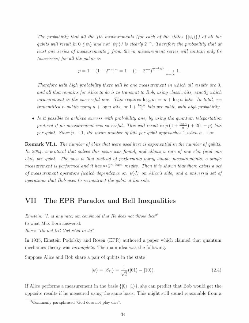
The probability that all the jth measurements (for each of the states |ψi〉) of all the

qubits will result in 0 (|ψi〉 and not |ψ⊥i 〉) is clearly 2−n. Therefore the probability that at

least one series of measurements j from the m measurement series will contain only 0s

(successes) for all the qubits is

p = 1 − (1 − 2−n)m = 1 − (1 − 2−n)2n+log n −→n→∞

1.

Therefore with high probability there will be one measurement in which all results are 0,

and all that remains for Alice to do is to transmit to Bob, using classic bits, exactly which

measurement is the successful one. This requires log2m = n + logn bits. In total, we

transmitted n qubits using n+ log n bits, or 1 + lognn

bits per qubit, with high probability.

• Is it possible to achieve success with probability one, by using the quantum teleportation

protocol if no measurement was sucessful. This will result in p(1 + logn

n

)+ 2(1 − p) bits

per qubit. Since p→ 1, the mean number of bits per qubit approaches 1 when n→ ∞.

Remark VI.1. The number of ebits that were used here is exponential in the number of qubits.

In 2004, a protocol that solves this issue was found, and allows a rate of one ebit (and one

cbit) per qubit. The idea is that instead of performing many simple measurements, a single

measurement is performed and it has ≈ 2n+logn results. Then it is shown that there exists a set

of measurement operators (which dependence on |ψ〉!) on Alice’s side, and a universal set of

operations that Bob uses to reconstruct the qubit at his side.

VII The EPR Paradox and Bell Inequalities

Einstein: “I, at any rate, am convinced that He does not throw dice”3

to what Max Born answered:

Born: “Do not tell God what to do”.

In 1935, Einstein Podolsky and Rosen (EPR) authored a paper which claimed that quantum

mechanics theory was incomplete. The main idea was the following.

Suppose Alice and Bob share a pair of qubits in the state

|ψ〉 = |β11〉 =1√2(|01〉 − |10〉). (2.4)

If Alice performs a measurement in the basis |0〉, |1〉, she can predict that Bob would get the

opposite results if he measured using the same basis. This might still sound reasonable from a

3Commonly paraphrased “God does not play dice”.

34

classic point of view, since you might think that the bits were in opposite direction in advance,

and the measurement only revealed that. However the following property is problematic in this

context.

Property VII.1. For each orthonormal basis of H2, |v〉, |v⊥〉, the following holds:

|β11〉 =1√2(|vv⊥〉 − |v⊥v〉),

up to a global phase.

Therefore, for each basis in which Alice performs the measurement, she knows that afterwards

Bob will measure the opposite, using the same basis!

The members of EPR have found this issue problematic. Why? In their view, a physical theory

must obey the “local realism” paradigm:

Reality every measurable quantity must have a single value that does not depend on perform-

ing the measurement itself.

Locality performing a measurement in some place cannot immediately change the results of

another measurement in another distant location.

Suppose we agree with EPR, and these two properties indeed hold. If Alice and Bob share the

EPR pair (2.4), then Alice can measure her qubit in the basis |0〉, |1〉, and Bob can measure

his qubit in the basis |+〉, |−〉 at the same time. But due to Property VII.1, this means that

Alice and Bob together know the measurement result of (say) Alice’s qubit in two different

bases, which stands in contradiction to the postulates of quantum mechanics! Unless of course,

there is no fixed value to a measurable quantity before a measurement is performed (no reality),

or measurement in one place can instantly effect a measurement result in a remote place (no

locality). Therefore, either that one of the assumptions of the local realism paradigm is wrong,

or the quantum mechanics theory is not complete. Various experiments were designed and

carried out to resolve this issue. The basic idea behind them is to put some constraints (a.k.a.

Bell inequalities; see Section VII) on the statistical result of the experiment under the local

realism paradigm, and then find a way to do better with a quantum protocol using a shared

entangled state (e.g., the EPR state). These experiments were clearly on the side of quantum

mechanics.

Let us first analyze this from an information theoretic perspective: did Alice’s measurement

convey information to Bob?

We saw earlier that Bob’s r.d.m. is given by

ρ(2) = tr1(ρ) = I/2.

35

What is ρ(2) - Bob’s d.m. after Alice’s measurement?

Alice measures |v〉 w.p. p(v) = 1/2, and Bob will be in state |v⊥〉. Therefore Bob’s d.m. after

Alice measures v is

ρ(2)

v⊥= |v⊥〉〈v⊥|,

and after Alice measures v⊥:

ρ(2)v = |v〉〈v|,

and in total:

ρ(2) =1

2ρ

(2)

v⊥+

1

2ρ(2)v =

1

2

[|v⊥〉〈v⊥| + |v〉〈v|

]= I/2 = ρ(2),

exactly as before the measurement! Hence, from an information theoretic perspective nothing

has happened at Bob’s side as a result of Alice’s measurement!

This idea can be generalized further:

Theorem VII.1 (Locality). Let AB be a composite system in state ρAB. Then any quantum

operation (including unitary and measurements), performed on the system A alone, will not

change the r.d.m. ρB = trA(ρAB) of system B.

Remark VII.1.

• For each measurement in system A, we get a different ensemble in system B, but all such

ensembles have the same d.m. - the r.d.m. of B before the measurement.

• It can be deduced from the above that if there is no communication between A and B, we

may always assume that system A was measured in some basis, from system B’s point of

view. This is called the Principle of Implicit Measurements.

• In general an operation in system A does not convey information to system B, and there-

fore does not imply communication at a speed greater than the speed of light.

A Bell Inequality

Consider the following experiment: Alice and Bob get the (classical) bits a and b respectively.

These bits are selected uniformly in an i.i.d. manner. Alice and Bob are each required to

declare a bit, so that the following holds true:

a = b = 1, Alice and Bob declare the same bit value,

o.w. Alice and Bob declare different bit values.

It is not difficult to see that in the classical case they cannot succeed with probability greater

than 75% (even if they use common randomness). This bound is a Bell inequality (one of

36

1u

0u

0v

1v

8π

8π

8π

Figure 2.2: Measuring bases for Alice and Bob

several), and it turns out that it can be violated when using quantum states, as demonstrated

by the following algorithm.

Algorithm VII.1. Assume that Alice and Bob share the singlet state |β11〉 , 1√2(|01〉 − |10〉).

We define two measurement bases for Alice and Bob, depicted in Fig. 2.2.

Alice: |0〉〈u0|, |1〉〈u⊥0 |, |0〉〈u1|, |1〉〈u⊥1 |;

Bob: |0〉〈v0|, |1〉〈v⊥0 |, |0〉〈v1|, |1〉〈v⊥1 |.

Alice and Bob choose what measurement to use and what bit to declare, according to:

• Alice measures her qubit using the basis |0〉〈ua|, |1〉〈u⊥a |, according to the value of her

cbit a.

• Bob measures his qubit using the basis |0〉〈vb|, |1〉〈v⊥b |, according to the value of his cbit

b.

• Alice and Bob declare on their measurement result: 0 if |0〉 was the outcome of the mea-

surement, and 1 otherwise.

Probability of success analysis:

We shall analyze the probability of success for all possible a, b values.

a = b = 0: In this case, success is achieved when Alice and Bob declare different bits. Assume

Alice measured 0 (|u0〉). Bob is now at state |u⊥0 〉. The chances for success is the probability

that Bob measures 1 (|v⊥0 〉). The probability for that is

37

|〈u⊥0 |v⊥0 〉|2 = cos2(π

8) ≈ 0.85.

(The probability of success, in case Alice measures 1 (|u⊥0 〉), is identical)

a = 0, b = 1, a = 1, b = 0: The calculations in these cases are similar and yield the same

result.

a = b = 1: Here, the goal is to output the same bit. If Alice measured 0 (|u1〉), then the chance

for success is again,

|〈v1|u⊥1 〉|2 = cos2(π

8) ≈ 0.85.

(Again, the probability of success, in case Alice measures 1 (|u⊥1 〉), is identical)

We see here that the mentioned Bell inequality is violated, since the described strategy results

in chances of 85% > 75% for success.

Remark VII.2. The measurement of Alice did not convey any information to Bob or vice

versa, but correlation was present between their measurement results, due to their common ebit.

Corollary 2.2. At least one of the principles, reality or locality, does not hold. This is be-

cause the coexistence of both principles brings us back to classical physics, under which Bell’s

inequalities hold. These inequalities can be violated however, in the framework of quantum

mechanics.

38

Chapter 3

Quantum Compression

Summary by Shai Machnes.

I The Quantum Compression Problem

Definition I.1 (Discrete Memoryless Quantum Source). A Discrete Memoryless Quantum

Source is an ensemble |ψi〉 , pimi=1 in a d-dimensional Hilbert spaceHd with d.m. ρ =∑

i pi |ψi〉〈ψi|.

Remark I.1. A source is defined by an ensemble and not by a density matrix. However, as we

discuss later in Theorem I.1, the source can be equivalently defined via the d.m. alone.

In this chapter we address the basic question of quantum compression: How many qubits are

needed (on average) per input state dimension (log2 (d)), to represent the the source “reliably”?

First, we need to define a notion of reliability, or fidelity, in the quantum setting.

I.1 Fidelity

Definition I.2 (Fidelity). The fidelity between two pure quantum states, |ψ〉 and |φ〉, is defined

as

F (|ψ〉 , |φ〉) , |〈φ| ψ〉|2 .

Suppose we compress the state |ψ〉, and get the reconstructed state |φ〉. Then, after preforming a

Von-Neumann measurement with the operators |ψ〉〈ψ| , I − |ψ〉〈ψ|, we reproduce the source

state |ψ〉 with probability 0 ≤ F (|ψ〉 , |φ〉) = |〈φ| ψ〉|2 ≤ 1 .

39

Definition I.3 (Fidelity between pure and mixed states). The fidelity between a pure state |ψ〉and a mixed state ω with orthonormal decomposition ω =

∑i qj |ϕj〉〈ϕj| is defined as

F (|ψ〉, ω) ,∑

j

qj |〈ψ|ϕj〉|2 =∑

j

qj〈ψ|ϕj〉〈ϕj|ψ〉 = 〈ψ|ω|ψ〉 .

This definition suits the case where a single pure qubit |ψ〉 is reconstructed by an ensem-

ble/mixed state ω. We generalize the definition of fidelity further, to match the case of an

ensemble of pure states |ψi〉 that is reconstructed by an ensemble of corresponding mixed

states ωi.

Definition I.4 (Average Fidelity). The average fidelity between the ensemble of pure states

|ψi〉, pi and the corresponding mixed states ωi is

F (avg) ,∑

i

pi 〈ψi|ωi |ψi〉 .

Property I.1 (Fidelity properties). The following properties are true for all the three afore-

mentioned definitions of fidelity (Definition I.2, Definition I.3, Definition I.4):

• 0 ≤ F ≤ 1.

• F is 1 for identical states.

• F is 0 for orthogonal states.

• F → 1 implies that any measurement performed on the reconstructed system will result

in a probability distribution approaching (in total variation) that obtained by performing

the same measurement on the original system, making the two systems “arbitrarily close”

to being indistinguishable.

I.2 Quantum Coding Scheme

A quantum coding scheme of rate R (qubits/state) and block length n for a quantum (memo-

ryless) source over Hd is denoted C (Hd, n, R,E,D).

Where the encoder E is a mapping

E : H⊗nd −→ ∆ (H2nR)

and the decided decoder D is a mapping

D : ∆ (H2nR) −→ ∆(H⊗nd

),

and where ∆(·) is the set of all density matrices over its argument Hilbert space.

40

Remark I.2. E and D must satisfy some conditions we will define in the sequel, in order to

be feasible by the laws of quantum mechanics

Definition I.5 (Fidelity of Coding Scheme). Given an alphabet A and encoding scheme C, the

fidelity of the coding scheme is defined as

F (A, C) ,∑

(ψi,pi)∈A⊗n

piF(ψi, D E (|ψi〉)

)=

∑

(ψi,pi)∈A⊗n

pi〈ψi|D E (|ψi〉) |ψi〉 ,

where A⊗n is an ensemble of tensor products of n identical copies of the source A, with the

associated multiplicative probabilities.

Definition I.6 (Achievable Rate). A rate R is achievable if there exists a sequence of coding

schemes of fixed rate R such that

limn→∞

F (A, Cn) = 1 .

As usual, we will be interested in the infimum over all achievable rates.

Example I.1. Consider an ensemble of |0〉, |+〉 with equal probabilities. From a classically

point of view, it seems no compression is possible. However, note that these states are non-

orthogonal and hence are indistinguishable, according to Theorem III.2, Chapter 1. Intuitively,

this fact can be used for compression, as the decoder is not required to distinguish between the

two.

One can show that the best “guess”, without information being conveyed, is |0〉 = cos(π8

)|0〉 + sin

(π8

)|1〉,

whereas the worst guess is |1〉 = sin(π8

)|0〉 − cos

(π8

)|1〉. see Fig. I.1. Note that a guess of a

constant qubit corresponds to R = 0.

To evaluate an achievable rate for this scheme, when n→ ∞, let us look on the set

B =|0〉, |1〉

⊗n

and express the ensemble states with respect to this basis:

|0〉 = cos(π

8

)|0〉 + sin

(π8

)|1〉

|+〉 = cos(π

8

)|0〉 − sin

(π8

)|1〉 .

Now we can easily express a source block of length n, |ψ〉 ∈ A⊗n (|ψ〉 = |ψi1〉|ψi2〉 . . . |ψin〉), in

this basis:

41

|0〉

|1〉

|+〉

|0〉

|1〉

Figure 3.1: Best and worst compressions of single qubit with R = 0

|ψ〉 =(cos(π

8

)|0〉 ± sin

(π8

)|1〉)⊗ · · · ⊗

(cos(π

8

)|0〉 ± sin

(π8

)|1〉)

=∑

φ∈0,1n± sin

(π8

)n1(φ)

cos(π

8

)n−n1(φ)

|φ〉 ,

where n1(φ) denotes the number of 1s in φ, where φ runs over all sequences of |0〉, |1〉.

Remark I.3. All the source sequences have equal probabilities. If we would have taken non-

equal probabilities for |0〉 and |+〉 we would have seen typical and non-typical sequences here,

unlike this case, in which all sequences are typical.

The fidelity between |ψ〉 and some |φ〉 is

|〈ψ|φ〉|2 =(sin2

(π8

))n1(φ) (cos2

(π8

))n−n1(φ)

= λn1(φ)(1 − λ)n−n1(φ) ,

where λ , sin2(π8

). Hence, the projection over |φ〉 can be viewed as the probability of a clas-

sical binary source A sequence with probabilities A ∼ (λ, 1 − λ), consisting of n1(φ) ones and

(n− n1(φ)) zeros. From the AEP, there are ∼ 2nhb(λ) typical sequences of A with probability

approaching 1, for n→ ∞.

42

Corollary 3.1. There are ∼ 2nhb(λ) vectors in B which span a typical subspace, with the property

that each source sequence has a projection on this subspace with length (arbitrarily) close to 1,

i.e., fidelity close to 1. Hence this scheme give rise to the achievable rate:

R = hb(λ)

Remark I.4. It can be shown that the following equality holds: ρ = |ψ〉〈ψ| = (1 − λ)|0〉〈0| + λ|1〉〈1|,meaning we were able to compress the source to the (classical) entropy of the eigenvalues of its

d.m.. This is true for any quantum source, as we see next in Theorem I.1.

I.3 AEP - Asymptotic Equipartition Property

Definition I.7 (Von-Neumann Entropy). The Von-Neumann (quantum) entropy of a quantum

source with d.m. ρ is

S (ρ) , −∑

i

λi log λi = −tr (ρ log ρ) , (3.1)

where λi are the eigenvectors of ρ.

Proof. The last equality holds since ρ is a positive symmetric matrix, and hence can be rep-

resented as ρ = UDU †, for some diagonal matrix D with a non-negative diagonal and uni-

tary matrix U. Thus, log ρ = U logDU † and tr(ρ log ρ) = tr(UD logDU †) = tr(D logD) =∑

i λi log λi

Remark I.5.

• The eigenvalues λi always constitute a probability vector.

• S(ρ) = H(λi) ≤ H(pi), where pi are the ensemble probabilities; equality holds

iff the ensemble states are orthogonal, since in this case we get a classical source. The

difference between the two flanks may serve as a measure for the amount of separability

between the ensemble states.

• S(ρ) = H(λi) ≤ log d, where d is the dimension of the system.

Theorem I.1 (The Quantum Coding Theorem, Schumacher 1995 [12]). Let A be a quantum

source with density matrix ρ and let ǫ, δ > 0.

1. Direct: For every large enough n, there exists a coding scheme of rate R < S (ρ) + δ,

and fidelity F > 1 − ǫ.

43

2. Converse: For every large enough n, the fidelity of any coding scheme with R < S (ρ)−δsatisfies F < 1 − ǫ.

Proof. 1. Achievability:

ρ is a positive matrix with trace equal to 1 and hence the following orthogonal decomposition

ρ =∑

i

λi |vi〉〈vi| , (3.2)

for some orthonormal basis vi and where all eigenvectors are non-negative and satisfy:∑

i λi = 1. Define a classical source A, such that

A = λi, |vi〉 .

This source has a (classical) entropy of

H(A)

= H (λi) = S (ρ) .

Let us now examine the source

An ≡ A⊗n

with the associated density matrix ρ⊗n.

According to the AEP, for every ǫ, δ > 0 there exists a large enough n such that there is a

subspace of 2n(H(A)+δ) = 2n(S(ρ)+δ) typical sequences with an overall fidelity of at least 1 − ǫ.

Therefore, there are 2n(S+δ) typical orthonormal eigenvectors of ρ⊗n, whose corresponding eigen-

values sum is equal or greater than 1 − ǫ. Denote this typical subspace by T = T (n, ǫ, δ).

Encoding Scheme:

The encoding scheme acts on An.

1. Project the data onto the subspace T , using the POVM PT , I − PT, where PT is the

projector on T .

2. If the result is not in T (i.e., belongs to T⊥ - the “non-typical” case), then encode using

some predefined state |err〉 ∈ T . This way an “error” is declared. Denote the state after

these two stages by |φ〉.

3. Apply the following unitary operator, which maps the typical subspace into n (S + δ)

qubits:

U |φ〉 =

|ψφ〉 |0rem〉 |φ〉 ∈ T

unitary completion of U otherwise

44

where |ψφ〉 is a state composite of n (S + δ) qubits, whereas |0rem〉 = |0 . . . 0〉 makes the

remaining n− n (S + δ) qubits.

Note: This is simply an enumeration of the elements in T .

4. Send the first n (S + δ) qubits of the resulting state.

Decoding Scheme:

1. Pad the state |ψφ〉 with |0rem〉.

2. Apply U † ≡ U−1.

Performance Analysis The encoding rate is clearly R = S (ρ) + δ. We shall now prove that

F → 1.

Assume some state |a〉 ∈ An. This state can be decomposed into a sum of a vector |ta〉belonging to the typical subspace T and a vector |t⊥a 〉 belonging to T⊥:

|a〉 = αa |ta〉 + βa∣∣t⊥a⟩

.

After measuring with the POVM PT , I − PT, and replacing the resulting state with the

predefined state |err〉, in case it belongs to T⊥, we are left with the mixed state

ωa = |αa|2 |ta〉〈ta| + |βa|2 |err〉〈err|

, which is also the state, recovered at the decoder. By calculating the fidelity between the

(original) source state |a〉 and the quantized state ωa, we arrive to the following lower bound:

F (|a〉 , ωa) = 〈a|ωa |a〉= |αa|2 |〈a| ta〉|2 + |βa|2 |〈a| err〉|2

≥ |αa|2 |αa|2 = |αa|4 ≥ 2 |αa|2 − 1

= 2 〈a|PT |a〉 − 1 = 2tr (PT |a〉〈a|) − 1 ,

where the second inequality follows from the fact that |αa|4 − 2|αa|2 + 1 = (|αa|2 − 1)2 ≥ 0.

To evaluate the fidelity of the coding scheme, we average over the ensemble:

45

F ≥∑

(|a〉,pa)∈An

pa (2tr (PT |a〉〈a|) − 1)

= 2∑

(|a〉,pa)∈An

tr (PTpa |a〉〈a|) − 1

= 2tr

PT

∑

(|a〉,pa)∈An

pa |a〉〈a|

− 1

= 2tr(PTρ

⊗n)− 1

≥ 2 (1 − ǫ) − 1

= 1 − 2ǫ ,

where the second inequality holds since ρ⊗n and PT are diagonal w.r.t. the same basis, due

to the definition of T , where PT has 2n(S+δ) ones on its diagonal (and 2n(1−(S+δ)) zeros), which

correspond to a set of (the largest 2n(S+δ)) eigenvectors, on the diagonal of ρ⊗n, which sum up

to (1 − ǫ) or more.

Remark I.6.

• The suggested scheme provides a good fidelity without knowing the exact source state, but

rather only the d.m. of the ensemble. It is optimal for all sources with the same density

matrix. Hence, it is convenient to think of sources as density matrices.

• Nonetheless, high fidelity is maintained w.r.t. the true states emitted by the source, al-

though these are not known and could not be generally determined.

• Suppose that it is given that S(ρi) < S, where ρi are possible sources which satisfy

ρiρj = ρjρi, i.e., simultaneously diagonizable. Then, it is possible to construct a “uni-

versal” scheme, which allows to quantize all the sources with (arbitrarily) good fidelity by

considering a (polynomially) larger space, which consists of the intersection of the typical

sets of all the sources.1

2. Upper Bound:

We shall restrict our attention to unitary decoders only, since the proof for the general case is

much more complicated and lacks intuition. It can be found in [1].

1This is similar to the classical case, in which we consider all sources with bounded entropy, by taking all

types with smaller entropy, whose number is polynomial in n, and thus, does not produce any penalty

46

Remark I.7. |a〉 does not necessarily lay inside Λn.

The fidelity of the coding scheme can be upper bounded by:

F =∑

(pa,|a〉)∈An

pa〈a|ωa|a〉 ≤∑

(pa,|a〉)∈An

patr(PaPΛn) = tr

PΛn

∑

(pa,|a〉)∈An

pa|a〉〈a|

= tr

(PΛnρ

⊗n) .

(3.3)

If we denote by|ei〉d

n

i=1

the basis of the eigenvectors of ρ⊗n, with the corresponding eigenvalues

µi which satisfy, w.l.o.g, we can rewrite the upper bound of (3.3) into:

F ≤ tr(PΛnρ

⊗n) =

dn∑

i=1

µitr (PΛn|ei〉〈ei|) =

dn∑

i=1

µi〈ei|PΛn|ei〉.

Now observe the following two properties:

0 ≤ 〈ei|PΛn|ei〉 ≤ 1

dn∑

i=1

〈ei|PΛn|ei〉 =

dn∑

i=1

tr (PΛn|ei〉〈ei|) = tr(PΛnIn) = tr(PΛn) = 2nR .

Hence, there are at most 2nR non-zero (strictly positive) summands in (3.3), meaning that the

coding scheme fidelity can be further bounded by:

F ≤2nR∑

i=1

µi < ǫ , (3.4)

where the last inequality holds for large enough n and stems from the classical AEP: if we

consider a classical source A with probabilities equal to the eigenvalues of ρ, then one sees that

µi correspond to the probabilities of sequences of A of length n. Since we assumed R <

S(ρ) ≡ H(A), according to the (classical) AEP, the sum in (3.4) goes to zero, as exponentially

less than 2nH(A) sequences are being summed. See [4, ch. 3].

Remark I.8.

• No assumption was made on the encoding process. Hence, in the case that the encoder

is aware of the exact source state (“visible coding”), the optimal achievable rate cannot

improve over the case in which the encoder is ignorant of the exact state to be sent (“blind

coding”). This holds true for general decoders as well.

• While proving Theorem I.1, we proved the quantum AEP, stated in Chapter 4, Section I.

48

• A more general decoder cannot improve the achievable rate. Nevertheless, it may improve

the fidelity, at least for visible coding.

• The proof assumed block coding; however, there exists a converse for variable-length coding

as well.

• Quantum variable-length coding: Much more involved due to the entanglement that

might exist between the lengths of the code word and the information itself.

Example I.2. Given an orthonormal decomposition ρ =∑

i di|ei〉, one might want to

represent |ei〉, using log 1di

qubits. However, a quantum source state is, in general, a

superposition of |ei〉, and hence its length would be a quantum quantity, i.e., a super-

position of values (which is not necessarily integer!). Furthermore, a measurement of the

length may effect the source state. A solution to this problem was given by Schumacher

and Westmoreland.

• Variable-length coding does not proivde F = 1 (“lossless”), unless a classical channel

exists, on which the lengths of the codewords can be conveyed and the source is visible to

the encoder (which is aware of the code word lengths, without measuring). In this case it

is possible to achieve rate beneath S(ρ).

49

Chapter 4

Quantum AEP and Von-Neumann

Entropy Properties (Part I)

Summary by Y uval Kochman and Anatoly Khina.

I Quantum Asymptotic Equipartition Property

Theorem I.1 (Quantum AEP). Let ǫ, δ > 0.

Direct: for any n large enough there exists a typical linear subspace in H⊗nd T = T (n, ǫ, δ) of

dimension 2nS(ρ)+δ, which satisfies:

tr(ρ⊗nPT

)≥ 1 − ǫ. (4.1)

Converse: for every subspace T = T (n, ǫ, δ) in H⊗nd of dimension 2nS(ρ)−δ, there exists n large

enough, such that:

tr(ρ⊗nPT

)< ǫ. (4.2)

Remark I.1. This theorems implies that ρ⊗n contained in a space which is almost entirely

spanned by a subspace of dimension nS(ρ).

51

II Purification and Schmidt Decomposition

II.1 Purification

Proposition II.1. Suppose a state ρA of a quantum system A. It is possible to introduce another

system R and define a pure state |AR〉 for the joint system AR, such that:

ρA = trR (|AR〉〈AR|) . (4.3)

|AR〉 is the “purification” of ρA.

Proof. Suppose ρA has orthonormal decomposition ρA =∑

i pi|iA〉〈iA|. Introduce a system R

with the same state space as system A and with an orthonormal basis|iR〉. Define the state

|AR〉 ,∑

i

√pi|iA〉|iR〉

in composite system AR. Tracing out system B, we obtain:

trR (|AR〉〈AR|) = trR

(∑

i,j

√pipj|iAiR〉〈jAjR|

)=∑

i,j

√pipj|iA〉〈jA|trR

(|iR〉〈jR|

)

=∑

i,j

√pipj|iA〉〈jA| 〈iR|jR〉︸︷︷︸

δi,j

=∑

i

pi|iA〉〈iA| = ρA.

Thus |AR〉 is a purification of ρA.

Remark II.1.

1. According to this proposition one can suggest that only pure states exist, and view mixed

states as pure states where only part of the system is visible to us. This is a valid (and

sometimes useful) point of view.

2. The converse of this proposition was already seen earlier Chapter 2, Section IV: measuring

a pure state gives a mixed state if the result of the measurement is not known.

3. There is an infinite number of possible purifications of some (specific) mixed state, even

when using the same system R. This can be easily seen from the construction used in the

proof, which allows to use any orthonormal basis in R (there is an infinite number of such

bases). See home assignment.

4. Let |AR1〉 and |AR2〉 be two purifications of a state ρA to a composite system AR. Then

there exists a unitary transformation UR acting on system R, such that:

|AR2〉 = (IA ⊗ UR) |AR1〉

, where IA is the identity transformation.

52

5. The dimension of R is greater or equal to rk(ρA). And, as seen from the proof, no higher

dimension than that is needed.

II.2 Schmidt Decomposition

Theorem II.1. Let |ψ〉 be a pure state of a composite system AB. Then there exist two

orthonormal sequences|eAi 〉

,|fBi 〉

of systems A,B respectively, such that:

|ψ〉 =∑

i

λi|eAi 〉|fBi 〉,

where λi are real none-negative numbers satisfying∑

i λ2i = 1, known as “Schmidt coefficients”

and the number of strictly positive such coefficient is known as “Schmidt Number” and is denoted

by Sch(ψ).

Proof. Let|jA〉

,|kB〉

be two orthonormal bases of systems A,B respectively. Hence |ψ〉

can be represented, according to these bases, as∑

j,k αjk|jA〉|kb〉.

For the rest of the proof we shall introduce a new definition, a simple result that applies to it

and use the SVD.

Definition II.1 (Representation Operator). The representation operator (or matrix) of |ψ〉with respect to bases

|jA〉

,|kB〉

, is defined as

[|ψ〉] = [ψ] ,∑

j,k

|jA〉〈kB|.

Remark II.2. Note that [ψ] and |ψ〉 are isomorphic.

Proposition II.2. For every pair of unitary operators U, V acting on systems A,B respect.,

the following is true:

[(U ⊗ V )|ψ〉] = U [|ψ〉]V †. (4.4)

Proof of Prop. II.2.

(U ⊗ V )|ψ〉 =∑

j,k

αjk(U |jA〉

) (V |kB〉

).

Hence, according to Definition II.1, we have

[(U ⊗ V )|ψ〉] =∑

j,k

αjkU |jA〉〈kB|V † = U

(∑

j,k

αjk|jA〉〈kB|)V † = U [ψ]V †,

Which concludes the proof.

53

Theorem II.2 (Singular Value Decomposition). For every matrix A there exist unitary matri-

ces U, V and a diagonal matrix Λ with a none-negative diagonal, satisfying:

A = UΛV †. (4.5)

Using Theorem II.2, we can decompose [ψ] into

[ψ] = UΛV † (4.6)

for some unitary matrices U, V and a diagonal matrix Λ with a none-negative diagonal, the last

elements of whom we denote by λi. This allows us to define the pure state

|ϕ〉 =∑

i

λi|iA〉|iB〉. (4.7)

Using Definition II.1, we have

[ϕ] = Λ (4.8)

and by combining (4.6) and (4.8) we have

[ψ] = U [ϕ]V † = [(U ⊗ V )|ϕ〉] ,

where in the last equality we used Prop. II.2. Now using the isomorphism, mentioned in

Remark II.2 we obtain

|ψ〉 = (U ⊗ V )|ϕ〉 =∑

i

λi U |iA〉︸︷︷︸|eAi 〉

V |iB〉︸︷︷︸|fBi 〉

=∑

i

λi|eAi 〉|fBi 〉.

Finally note that the sequences|eAi 〉

,|fBi 〉

are orthonormal since U, V are unitary.

Corollary 4.1. The following equalities hold true:

ρA = trB (|ψ〉〈ψ|) =∑

i

λ2i |eAi 〉〈eAi |

ρB = trB (|ψ〉〈ψ|) =∑

i

λ2i |fBi 〉〈fBi |.

Hence, ρA and ρB have the same eigenvalues, which differ from zero, λ2i and the same dimension

Sch(ψ) = dim trB (|ψ〉〈ψ|).

Remark II.3.

1. A and B are not necessarily of the same dimension.

54

2. The sequences|eAi 〉

,|fBi 〉

are, in general, state-dependent. That is, they can vary,

depending on the state |ψ〉.1

3. The Schmidt coefficients (λi) (and hence also the Schmidt number) are invariant to local

unitary transformations.

4. Corollary 4.1 implies that if a system AB is in pure state, then both of its subsystems A

and B have the same VN entropy.

5. Purification can be thought of as a “correct” Schmidt basis selection. The state |AR〉 is

chosen such that its Schmidt basis in system A, viz. |eAi 〉, is the diagonalizing basis of ρA.

Moreover, the corresponding Schmidt coefficients are the square-roots of the eigenvalues

of ρA.

6. |AR1〉 and |AR2〉 are purifications of ρA in the system AR if and only if there exists a

Unitary UR acting on the R system such that |AR2〉 = (IA ⊗ UR)|AR1〉.

7. In purification, rank(R) ≥ ρA, and the minimal rank is always sufficient.

III Fidelity between Mixed States

In Definition I.3 we defined the fidelity between a pure state and a mixed state as

F (|ψ〉, ρ) , 〈ψ|ρ|ψ〉.

However a straightforward generalizing this definition to two mixed states would fail. Hence, a

different fidelity definition is needed.

Definition III.1. Let ρ and σ be two mixed states of system A. Then the fidelity between these

states is defined as

F (ρ, σ) , min|ψ〉∈AR

trR(|ψ〉〈ψ|)=ρ

max|ϕ〉∈AR

trR(|ϕ〉〈ϕ|)=σ

|〈ψ|φ〉|2 (4.9)

where ψ and ϕ are some purification of ρ and σ to system AR, respectively.

Remark III.1.

1. One can prove that

F (ρ, σ) = max|ϕ〉

|〈ψ|ϕ〉|2 (4.10)

holds for any fixed purification of ρ, and the maximization is over all purifications of σ.

1This can be seen in the proof of Theorem II.1, since the matrices U, V of the SVD depend on the exact

matrix being decomposed.

55

2. Note that the maximization in (4.10) is essential (unlike the outer minimization of (4.9))

since if we, for instance, were to use min instead of max in (4.10), we would approach 0

by taking dim(R) to infinity.

3. Since the exact purification of ρ ins not important (as long as we fix it and maximize with

respect to |ϕ〉), we can replace (4.9) with

F (ρ, σ) , max|ψ〉,|ϕ〉∈AR

|〈ψ|φ〉|2 , (4.11)

where the maximization is over all purifications |ψ〉, |ϕ〉 of ρ, σ respectively.

4. (4.11) suggests that fidelity is symmetric in its arguments.

Theorem III.1 (Uhlmann’s Theorem). Suppose ρ and σ are two (mixed) states of the same

system A. Then the fidelity between these two states satisfies:

F (ρ, σ) =

[tr

(√ρ

12σρ

12

)]2

. (4.12)

Remark III.2. (4.12) is reduced to the previously defined fidelity between a pure state and a

mixed state (see Definition I.3, Chapter 3)

F (|ψ〉, ρ) =[tr(√

〈ψ|ρ|ψ〉|ψ〉〈ψ|)]2

= 〈ψ|ρ|ψ〉 .

Theorem III.2. Suppose ρ and σ are two (mixed) states of the same system A. Then the

fidelity between these two states satisfies:

F (ρ, σ) = minEm

∑

m

√pmqm ,

where

pm , tr(ρEm)

qm , tr(σEm)

and the minimization is taken over all possible POVMs Em.

The proofs of Theorem III.1 and Theorem III.2 can be found in [11].

IV Quantum Source Coding of an Ensemble of Mixed States

Definition IV.1 (i.i.d. Mixed Source). An ensemble ρi, piMi=1 in a d-dimensional Hilbert

space Hd, whose probabilities pi are drawn in an i.i.d. manner.

56

If we denote by σn a source block of length n, i.e., σn = ρi1 ⊗ ρi2 ⊗ · · ·⊗ ρin , then we can define

the average fidelity between this ensemble and a reconstruction state σn as

F ,

M∑

i1,i2,...,in=1

P (σn)F (σn, σn) . (4.13)

Remark IV.1. This definition reduces to Chapter 3,Definition I.4, if all ρi are pure.

Theorem IV.1. Let ρi, piMi=1 be an i.i.d. mixed source. Then for any ǫ > 0, there exists n0,

such that for every n > n0 there exists a coding scheme with rate

R ≥ S(ρ) −∑

i

piS(ρi) (4.14)

and an average fidelity that satisfies F > 1 − ǫ, where ρ =∑

i piρi.

Remark IV.2.

1. The right-hand side of (4.14) is known as the Holevo quantity and is denoted by χ.

2. Since VN entropy is none-negative (Shannon entropy of the eigenvalues) we have S(ρ) ≥ χ

with equality iff all ρi are pure. Hence, in the case of an ensemble of mixed states, a rate

of S(ρ) is achievable but not optimal, whereas when all ρi are pure, the bound of (4.14)

reduces to Chapter 3, Theorem I.1.

3. The lower bound of (4.14) is not tight.

4. In the case of a pure-state source, S(ρ) was the optimal achievable rate both for visible and

blind coding, i.e., both when the encoder knows or is ignorant of the state he compresses.

In the case of mixed-states, there are cases in which a visible encoder achieves strictly

better rates than a blind one.

Example IV.1 (S(ρ) is not tight). Suppose we want to compress an ensemble composed of only

one mixed state ρ1. Obviously, one can achieve a rate R = 0 with fidelity F = 1. However,

S(ρ) is strictly positive in this case due to the “impurity” of ρ1. On the other hand, χ(ρ) = 0

in this case, implying the bound (4.14) being tight.

V Information Quantities and Properties

Definition V.1 (Quantum Relative Entropy). Let ρ and σ be two density matrices of the same

system A. Then the “quantum relative entropy” between ρ and σ is defined as:

S (ρ‖σ) , tr (ρ log ρ) − tr (ρ log σ) .

57

Theorem V.1 (Klein’s Theorem).

S (ρ‖σ) ≥ 0, (4.15)

with equality iff ρ = σ.

Proof. Decompose rho and σ to their orthonormal decompositions:

ρ =∑

i

pi|i〉〈i| , σ =∑

j

qj |j〉〈j|. (4.16)

Note that |i〉 and |j〉 are not (necessarily) the same basis. Hence we can rewrite the relative

entropy as

S (ρ‖σ) =∑

i

pi log pi −∑

i

〈i|ρ log σ|i〉,

using the identity tr(A) =∑

i 〈i|A|i〉.The decomposition in (4.16) implies 〈i|ρ = pi〈i|. Using this, we further the relative entropy:

S (ρ‖σ) =∑

i

pi log pi −∑

i

pi〈i| log σ|i〉

=∑

i

pi log pi −∑

i

pi〈i|(∑

j

log(qj)|j〉〈j|)|i〉

=∑

i

pi

[log pi −

∑

j

Cij log qj

],

where Cij , 〈i|j〉〈j|i〉 = |〈i|j〉|2 satisfies:

∑

i

Cij =∑

i

〈i|j〉〈j|i〉 = tr

(∑

i

|i〉〈i||j〉〈j|)

= tr (I|j〉〈j|) = 〈j|j〉 = 1,

∑

j

Cij = 1,

thus constituting a doubly-stochastic matrix. This enables us to define the probability vector

ri ,∑

j Cijqj in the sequel

S (ρ‖σ) =∑

i

pi

[log pi −

∑

j

Cij log qj

](a)

≥∑

i

pi

log pi − log

ri︷︸︸︷∑

j

Cijqj

=∑

i

pi[log pi − log ri

]=∑

i

pi logpiri

= D(p‖r) (b)

≥ 0 .

(a) is due to Jensen’s inequality and is held with equality iff C is a permutation matrix, i.e.,

ρ and σ have the same eigenvectors. Equality in (b) holds iff pi = qi for every i, viz. identical

eigenvalues. Thus equality in (4.15) holds iff ρ = σ.

58

Definition V.2. Let system AB be a quantum system in a state with entropy S(AB) ≡ S(A,B).

Then the conditional VN entropy is defiend as

S(A|B) , S(A,B) − S(B), (4.17)

and the quantum mutual information as

S(A;B) , S(A) − S(A|B) = S(A) + S(B) − S(A,B). (4.18)

Remark V.1. The quantum quantities of Definition V.2 are a natural generalization of the

parallel classical quantities. However, in the quantum case, the meaning of these quantities is

less apparent.

Example V.1. Let us look look on a Bell state |ψ〉 = 1√2(|00〉 + |11〉) of a composite system

AB, where the first qubit is of system A whereas the second one - of system B. Since |ψ〉 is a

pure state, its VN entropy is S(A,B) = 0. However its reduced density matrices ρA = ρB = I2

posses an entropy of S(A) = S(B) = 1, giving rise to the following, somewhat strange equalities:

S(A|B) = S(B|A) = −1 < 0 .

At first, it seems as though the conditional VN entropy (and consequently quantum mutual

information) has no operative meaning. Luckily this is not the case. It can be shown that:

1. S(B|A) ≥ 0 : Alice needs to transmit S(B|A) qubits, so that Bob will be able to reproduce

the mutual state (asymptotically with F → ∞) - as in the classical case.

2. S(B|A) : Bob can produce the composite state by himself and in addition |S(B|A)| ebits

for for future communication (assuming there exists a classical channel with unlimited

capacity).

V.1 Von-Neumann Entropy Properties

Property V.1.

0 ≤ S(A) ≤ log (dim(A))

where equality in the left inequality holds for a pure state and in the right one - for a maximally

mixed state.

Proof. Define the dimension of A by d , dim(A). The left inequality and the corresponding

equality condition are obvious. Let us prove the right inequality by looking at the following

59

relative entropy and applying Klein’s Theorem:

0 ≤ S

(ρA∥∥∥∥I

d

)= −S(ρA) − tr

(ρA log

I

d

)

= −S(ρA) − log1

d· tr(ρA) − tr(ρA log I︸︷︷︸

=0

) = −S(ρA) + log d ,

where in the last equality we used the fact that tr(ρA) = 1 for any density matrix.

Hence S(ρA) ≥ log d with equality iff ρA = Id

as indicated by (4.15).

Property V.2. If AB is in a pure state, then S(A) = S(B).2

Property V.3 (Additivity of Product States). S(ρ⊗ σ) = S(ρ) + S(σ).

Property V.4 (Projective Measurements Increase Entropy). Let Pi be some set of orthonor-

mal projectors and ρ some density matrix. Then the entropy of the state after the measurement

ρ′ ,∑

i PiρPi is at least as great as the original entropy, before measuring:

S(ρ′) ≥ S(ρ),

with equality iff ρ′ = ρ

Proof. By considering the relative entropy between ρ′ and ρ and applying Klein’s Theorem to

it, we have

0 ≤ S(ρ′‖ρ) = −S(ρ) − tr (ρ log ρ′) .

Let us now prove that −tr(ρ log ρ′) = S(ρ′). Using the relations of projective operators P 2i = Pi

and the completeness relation∑

i Pi =∑

i P2i = I, we obtain

−tr (ρ log ρ′) = −tr

=I︷︸︸︷∑

i

P 2i ρ log ρ′

= −

∑

i

tr(P 2i ρ log ρ′

)= −

∑

i

tr (Piρ log ρ′Pi)

= −tr(∑

i

Piρ log ρ′Pi

).

Note that Pj commute ρ′ and hence with log ρ′ as well. This is true due to PiPj = Piδi,j :

ρ′Pj =

(∑

i

Piρ′

)Pj = PjρPj = Pjρ

′.

Thus

−tr (ρ log ρ′) = −tr(ρ′ log ρ′) = S(ρ′).

Thus we proved that S(ρ′) ≥ S(ρ), with equality iff ρ = ρ′

2This was already stated and proved in Remark II.3.

60

Remark V.2. A none-projective measurement might decrease entropy.

Property V.5 (Subadditivity). Let A and B be distinct quantum systems in a joint state ρAB.

The the following inequality holds:

S(A,B) ≤ S(A) + S(B) (4.19)

with equality iff ρAB = ρA ⊗ ρB.

Proof. We shall look at the entropy between the joint state ρAB and the tensor state ρA ⊗ ρB

and apply Klein’s Theorem:

0 ≤ S(ρAB

∥∥ρA ⊗ ρB)

= −S(ρAB) − tr(ρAB log(ρA ⊗ ρB)

).

Let us consentrate on the second elemnt on the right-hand side:

tr(ρAB log(ρA ⊗ ρB)

)= tr

(ρAB log

(ρA ⊗ I)(I ⊗ ρB)

)

= tr(ρAB log(ρA ⊗ I)

)+ tr

(ρAB log(I ⊗ ρB)

),

where the last equality is true since the identity operator can be decomposed into an orthonor-

mal decomposition by any orthonormal basis.

Now using the fact that tr(•) = trA(trB(•)

), we come to

tr(ρAB log(ρA ⊗ I)

)+ tr

(ρAB log(I ⊗ ρB)

)= tr

(ρA log ρA

)+ tr

(ρB log ρB

)= −S(A) − S(B).

Combining all results and leads to the desired result.

Remark V.3. Note that in the course of the proof we also proved the following identity:

S(A;B) = S(A) + S(B) − S(A,B) = S(ρAB‖ρA ⊗ ρB).

61

Chapter 5

Von-Neumann Entropy Properties

(Part II)

Summary by Y ael Ben−Haim.

I Further Properties of the Von-Neumann Entropy

The triangle inequality is the quantum analogue of the classical inequality H(X, Y ) ≥ H(X).

It states the following.

Property I.1 (Triangle (Araki-Lieb) inequality). For any pair of systems A and B,

S(AB) ≥ |S(A) − S(B)| .

Proof. Introduce a system R that purifies the system AB. The subadditivity property (Prop-

erty V.5, Chapter 4) implies that

S(R) + S(A) ≥ S(AR) .

Since the system ABR is pure, by Property V.2, Chapter 4,

S(R) = S(AB)

and

S(AR) = S(B) .

Substituting (I) and (I) in (I), we obtain

S(AB) ≥ S(B) − S(A) .

63

Symmetrical arguments show that

S(AB) ≥ S(A) − S(B),

which completes the proof.

Property I.2. Let pi, ρi be an ensemble of states. Classical information theory is obtained

when the states ρi are pure and orthogonal. Otherwise, the incapability to distinguish between

states increases the uncertainty. This is made precise in the following theorem.

Let pi, ρi be an ensemble of states. Then

S(∑

i

piρi) ≤∑

i

piS(ρi)

︸︷︷︸penalty for

indistinguishability

+H(pi),

with equality if and only if the states ρi are orthogonal, i.e., they have supports on orthogonal

spaces.

Proof. We prove here only that orthogonality implies equality. The rest is proved in the home

assignment.

Letλjijand

|eji 〉jbe the eigenvalues and orthogonal eigenvectors of ρi. The orthogonality of

the states ρi implies thatpiλ

ji

i,j

are the eigenvalues of∑

i piρi with orthonormal eigenvectors|eji 〉. Hence

S

(∑

i

piρi

)= −

∑

i,j

(piλ

ji

)log(piλ

ji

).

Since∑

j λji = 1 for all i, we obtain

S

(∑

i

piρi

)= −

∑

i

pi log pi −∑

i

pi∑

j

λji log λji (5.1)

= H(pi) +∑

i

piS(ρi) . (5.2)

Property I.3 (Concavity). Let pi, ρi be an ensemble of states. Then

S(∑

i

piρi) ≥∑

i

piS(ρi) .

64

Proof. Let A be the system of the states ρi. Introduce a system B whose state space has an

orthonormal basis |i〉, with one-to-one correspondence to the states ρi and define the composite

state:

ρAB =∑

i

piρi ⊗ |i〉〈i| .

Then

S(A) = S

(∑

i

piρi

)

and

S(B) = S

(∑

i

pi|i〉〈i|)

= H(pi) .

Remark I.1. The states ρi are not necessarily orthogonal, whereas the |i〉〈i| - are. Hence,

the states ρi ⊗ |i〉〈i| are orthogonal as well.

Since the states ρi ⊗ |i〉〈i| are orthogonal, we have, according to Property I.2

S(AB) = S(ρAB) =∑

i

piS(ρi ⊗ |i〉〈i|) +H(pi) .

By Property V.3, Chapter 4,

S(AB) =∑

i

piS(ρi) +∑

i

piS(|i〉〈i|) +H(pi) .

Since |i〉 is a pure state, we have S(|i〉〈i|) = 0, and

S(AB) =∑

i

piS(ρi) +H(pi)

follows. Applying Property V.5, Chapter 4: S(AB) ≤ S(A) + S(B), we obtain

∑

i

piS(ρi) ≤ S(∑

i

piρi) .

So far we have encountered two properties, Property I.1 and Property I.3, whose proofs involved

the introduction of an auxiliary system. This is a useful method in quantum information theory.

In Property I.3, B allows us to store the knowledge of the index i, which is unknown in A. In

other words, one can regard B as the system of the creator of the state of ρA.

Property I.4 (Strong subadditivity). For any triplet of systems A,B,C:

S(ABC) + S(B) ≤ S(AB) + S(BC) .

65

Remark I.2.

• All the known proofs to Theorem I.4 are very difficult, and none of them will be given

here. See [11, ch. 11.4] for a proof and references. In fact, strong subadditivity was an

open conjecture for five years (from 1968 until 1973).

• The conditions for equality are also involved. See [9].

• Atrong subadditivity is trivial in the classic case and holds with equality iff A→ B → C,

i.e., iff A,B,C form a Markov chain.

Property I.5 (Conditioning reduces entropy). For any triplet of systems A,B,C:

S(A|BC) ≤ S(A|B) .

Proof. By definition,

S(ABC) = S(A|BC) + S(BC)

and

S(B) = S(AB) − S(A|B) .

The claim follows by substituting (I) and (I) in (I.4).

Corollary 5.1. Property I.5 implies that quantum conditional mutual information is non-

negative.

The following property follows easily from Property I.4.

Property I.6 (Discarding a system does not increase mutual information). For any triplet of

systems A,B,C:

S(A;B) ≤ S(A;BC) .

Property I.7 (Unitary operators preserve entropy). For any state ρ and unitary operator U :

S(ρ) = S(UρU †) .

Proof. Since U is unitary, the set of eigenvalues of ρ is equal to the set of eigenvalues of UρU †.

The claim follows from the definition of entropy.

The following property follows immediately from Property I.7 and the definition of mutual

information (Definition V.2, Chapter 4).

66

Property I.8 (Local unitary operators preserve mutual information). Let UA, UB be unitary

operators on systems A and B, respectively. Denote by A′, B′ the systems obtained from applying

UA ⊗ UB to AB. Then

S(A;B) = S(A′;B′) .

Property I.9 (Local measurements do not increase mutual information). Suppose that systems

A,B are measured locally and denote by A′, B′ the systems after these local measurements. Then

S(A′;B′) ≤ S(A;B) ,

if the outcomes of the measurements are not known.

Proof. A measurement is equivalent to an introduction of an auxiliary system, followed by a

unitary operation and the discarding of the auxiliary system, afterwards. By Property I.8,

the unitary operation preserves mutual information; by Property I.6, discarding the auxiliary

system does not increase mutual information, which completes the proof.

The following three properties are difficult to prove and therefore are state without such.

Property I.10 (Quantum relative entropy is jointly convex). Let ρi and σi be some state

sets and pi - a set of numbers. Then,

S

(∑

i

piρi||∑

i

piσi

)≤∑

i

piS(ρi||σi) .

Property I.11 (Monotonicity of relative entropy). Let ρAB, σAB be any two states in a com-

posite system AB. Then

S(ρA||σA) ≤ S(ρAB||σAB) .

Property I.12 (Concavity of conditional entropy). Let ρAB be any state in a composite system

AB. Then the conditional entropy S(A|B) is concave in ρAB.

II Accessible information

We have seen that it is impossible to distinguish between non-orthogonal states (or clone such).

Hence, we would like to quantify how much, two states, are distinguishable.

Consider the following scenario: a classical source X with probability distribution (p0, . . . , pn−1)

is encoded to the quantum mixed states (ρ0, . . . , ρn−1), respectively. Alice chooses an index

x ∈ 0, . . . , n − 1 with probability pi, and sends the corresponding state ρi to Bob. Bob

performs a measurement, resulting in a classical random variable Y , whose possible values are

67

in the range 0, . . . , m−1. The amount of information that Bob acquires about X is I(X;Y ).

Obviously, Bob should choose the POVM that maximizes I(X;Y ), as the (classical) MI is a

good measure for the information acquired by measurement: X can be perfectly reconstructed

iff I(X;Y ) = H(X); according to Fano’s inequality:

hb(pe) + pe log(n− 1) ≥ H(X|Y )︸︷︷︸I(X;Y ) = H(X) −H(X|Y )︸︷︷︸ .

This brings us to the following definition.

Definition II.1 (Accessible information). With the setting described above, the accessible in-

formation is defined as

Iacc , maxEy

I(X;Y ),

where the maximization is over all possible POVMs Ey.

Our task is to estimate the amount of accessible information. We first note that Iacc ≤ H(X),

with strict inequality when the states ρi are not orthogonal. We proceed to the introduction of

a more sophisticated estimate.

Theorem II.1 (The Holevo bound). With the setting described above, we have

Iacc ≤ χ,

where ρ =∑

x pxρx and χ , S(ρ)−∑x pxS(ρx) is the “Holevo quantity”; equality holds iff ρxcommute.

Proof. Let us denote the measurement operators by Mym−1y=0 , i.e., Ey = M †yMy. Recall that

the state after the measurement is

ρ′ =∑

y

MyρM†y .

Define the following three systems:

• P (“preparation system”) - a system with orthonormal basis |x〉n−1x=0, in correspondence

to the values of X.

• Q (“storing system”) - the system that Alice gives to Bob, i.e., the system of the states

ρx.

• R (“results accumulating system”) - a system with orthonormal basis |y〉m−1y=0 , in corre-

spondence to the values of P .

68

Alice and Bob prepare the following state:

ρPQR =∑

x

px|x〉〈x| ⊗ ρx ⊗ |0〉〈0| .

Remark II.1. The part px|x〉〈x| ⊗ ρx represents the choice and encoding of x by Alice, while

|0〉〈0| represents the initialization of R, done by Bob. Tracing-out PR, we receive exactly the

system that is sent by Alice to Bob.

Define unitary operators on the system R:

Ty|i〉 = |i+ y〉, (5.3)

where addition is modulo m; |i〉 orthonormal basis; note that (5.3) implies T †y |i〉 = |i− y〉.

Assertion II.1. The set My ⊗ Ty is a set of measurement operators on QR.

Proof. (Assertion)

Indeed, it is easy to check that My ⊗ Ty ≥ 0, and

∑

y

(My ⊗ Ty)(My ⊗ Ty)† =

∑

y

MyM†y ⊗ TyT

†y (5.4)

(a)=

(∑

y

MyM†y

)⊗ IR (5.5)

(b)= IQ ⊗ IR = IQR, (5.6)

where (a) is true because Ty is unitary for all y, and (b) is because My is a set of measure-

ment operators, and thus∑

yMyM†y = IQ due to the completeness equation (Postulate IV,

Chapter 4).

Thus, we can perform a measurement of ρPQR with the set I ⊗My ⊗ Ty, to obtain the state

ρP′Q′R′

=∑

x

∑

y

px|x〉〈x| ⊗MyρxM†y ⊗ |y〉〈y| .

The rationale behind this measurement is to measure Q with the set My and store the result

in R.

Remark II.2. Note that this measurement is consistent with a direct measurement of ρ:

ρQ′

= trP ′Q′

(ρP

′Q′R′)

= ... =∑

y

< MyρM†y .

69

To complete the proof, we show the following chain:

I(X;Y )(1)= S(P ′;R′)

(2)

≤ S(P ;Q)(3)= S(ρ) −

∑

x

pxS(ρx) .

1. We elaborate on ρP′R′

:

ρP′R′

=∑

x,y

tr(MyρxM†y)px|x〉〈x| ⊗ |y〉〈y|

=∑

x,y

py|xpx|x〉〈x| ⊗ |y〉〈y|

=∑

x,y

px,y|x〉〈x| ⊗ |y〉〈y| .

It follows that P ′R′ is a classical system, and hence:

S(P ′;R′) = I(X;Y ) .

2. We have

S(P ′;R′) ≤ S(P ′;Q′R′) ≤ S(P ;QR) = S(P ;Q),

where the first inequality follows from Property I.6, the second inequality follows from

Property I.9, and the final equality follows from the fact that R is in a product state with

PQ, see the home assignment.

3. We elaborate on ρPQ:

ρPQ = trR(ρPQR) =∑

x

px|x〉〈x| ⊗ ρx .

By Property 7,

S(PQ) = H(X) +∑

x

pxS(ρx)

Now,

S(P ) = H(X),

since

ρP =∑

x

px|x〉〈x|,

and

S(Q) = S(ρ),

since

ρQ =∑

x

pxρx .

70

Hence

S(P ;Q) = S(P ) + S(Q) − S(PQ) = S(ρ) −∑

x

pxS(ρx) . (5.7)

Remark II.3.

1. By Property I.3, χ is always non-negative.

2. As mentioned in the theorem, equality in the Holevo bound holds if and only if the states ρx

commute, i.e., they have the same set of eigenvectors. In this case, the bound is attained

using a Von-Neumann measurement in the joint basis.

3. An optimal measurement that attains the accessible information is generally not known.

Nevertheless, it is known [6] that there exists an optimal measurement of the form

Ey = αy|ψy〉〈ψy|,

where y = 0, . . . , m− 1 and

dimH ≤ m ≤ (dimH)2 .

4. Sometimes the bound can be far from tight. For example, if the states ρx are pure, then

the Holevo quantity is S(ρ), i.e., independent of the ensemble. Nevertheless, tighter (and

more involved) upper and lower bounds exist.

III The pretty good measurement (PGM)

For an ensemble px, ρxn−10 , the PGM is given by the POVM:

Ex = pxρ−1/2ρxρ

−1/2 ,

where ρ ,∑

x pxρx.

Let us now show that this is indeed a POVM. Denote by H the support of ρ. one easily verifies

that Ex ≥ 0 and ∑

x

Ex = ρ−1/2∑

x

pxρxρ−1/2 = ρ−1/2ρρ−1/2 = I ,

in H. if ρ is singular, we shall introduce an additional opeartor En to the POVM: En is nullified

on H and is equal to the identity operator outside it, i.e., En is the completion to I outside H.

Property III.1.

71

• If ρx are pure, then the probability of success, for the optimal measurement possible,

satisfies [5]:

P 2C(opt) ≤ PC(PGM),

which is pretty good!

• If ρx are pure and orthogonal, then the PGM is reduces to the optimal VN measurement.

• There are more scenarios in which the PGM is optimal.

72

Chapter 6

Quantum Channels and Classical

Capacity

Summary by Y uval Kochman and Anatoly Khina.

I Quantum Channels

Definition I.1 (Quantum Channel). A quantum channel is a mapping from ∆ (Hdin) to ∆ (Hdout):

E : ∆ (Hdin) −→ ∆ (Hdout) ,

which satisfies the property:

E(ρAB

)= trBD

(U(ρAB ⊗ |0CD〉〈0CD|

)U †), (6.1)

where ∆ (H) is defined as the set of all possible d.m. in H.

Remark I.1.

1. (6.1) suggests taking the system (AB) with a certain environment (CD), performing some

(unitary) interaction (U) between the two and “throwing” away part of the environment

(D) along with part of the system (B).

2. The ancilla state of the environment (|0CD〉〈0CD|) is assumed to be a pure state, since

otherwise one could convert it into such by applying purification to it, in the process of

which - enlarging the dimensions of the environment.

73

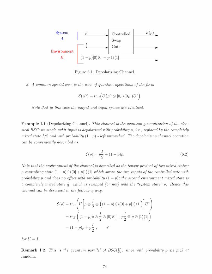
System

A

Environment

E

ρ

I2

(1 − p)|0〉〈0| + p|1〉〈1|

E(ρ)Controlled

Swap

Gate

Figure 6.1: Depolarizing Channel.

3. A common special case is the case of quantum operations of the form

E(ρA) = trE

(U(ρA ⊗ |0E〉〈0E|

)U †).

Note that in this case the output and input spaces are identical.

Example I.1 (Depolarizing Channel). This channel is the quantum generalization of the clas-

sical BSC: its single qubit input is depolarized with probability p, i.e., replaced by the completely

mixed state I/2 and with probability (1−p) - left untouched. The depolarizing channel operation

can be conveniently described as

E(ρ) = pI

2+ (1 − p)ρ. (6.2)

Note that the environment of the channel is described as the tensor product of two mixed states:

a controlling state (1− p)|0〉〈0|+ p|1〉〈1| which swaps the two inputs of the controlled gate with

probability p and does no effect with probability (1 − p); the second environment mixed state is

a completely mixed state I2, which is swapped (or not) with the “system state” ρ. Hence this

channel can be described in the following way:

E(ρ) = trE

(U

[ρ⊗ I

2⊗((1 − p)|0〉〈0| + p|1〉〈1|

)]U †

)

= trE

((1 − p)ρ⊗ I

2⊗ |0〉〈0| + p

I

2⊗ ρ⊗ |1〉〈1|

)

= (1 − p)ρ+ pI

2, X

for U = I.

Remark I.2. This is the quantum parallel of BSC(p2

), since with probability p we pick at

random.

74

I.1 Classical Capacity of a Quantum Channel

The aim of the encoder is to transmit as much classical information as possible to the decoder

over a quantum channel. Hence, this problem is close in mind to the classical (Shannon) channel

coding problem, only now the channel is quantum.

The most general (block-code) coding scheme, with block length n and rate R has the following

form:

Encoder: E :1, . . . , 2nR

−→ ∆

(H⊗ndin

).

Decoder: D : Em2nR

m=1.

This scheme takes the classical message, transforms it into a quantum channel state and mea-

sures it at the output. Our aim is, of course, to maximize the rate R of the scheme, such that

the probability of error would go to zero with the block-length n:

Pe =1

2nR

2nR∑

m=1

P

(D E

(E(m)

)6= m

)−→ ∞ .

Proposition I.1 (Classical-Classical Capacity). The classical capacity of a quantum channel

E is

CCC = maxpi,ρi

Iacc

(pi, E(ρi)

)(6.3)

when restricting the use to a product-state at the encoder:

E :1, . . . , 2nR

−→

n⊗

i=1

∆ (Hdin) (6.4)

and a decoder of the form

D : Em , Em =

n⊗

i=1

Em,i . (6.5)

Remark I.3. Constraints (6.4),(6.5) mean that no entanglement is exploited, not at the input

of the channel, nor in its output. Making this approach to the problem very “classical”.

Proof Sketch. For every channel instance, the maximum that can be achieved is Iacc and there

is no entanglement that can be exploited. Hence the effective channel is a classical channel

whose input can be “shaped” by selecting different ensembles pi, ρi.Remark I.4. From The Holevo bound Theorem II.1, (Chapter 5, the following upper bound on

Ccc holds

CCC ≤ maxpi,ρi

χ

(E ,pi, ρi

)

χ

(E ,pi, ρi

), S

(E(∑

i

piρi

))−∑

i

piS(E(ρi)

). (6.6)

75

Note that in general this bound is not tight Theorem II.1, Chapter 5. Nevertheless, by allowing

a general measurement, we can achieve the Holevo upper bound, as suggested by the following

theorem.

Theorem I.1 (HSW). The classical capacity of a quantum channel E , under a product-state

constraint (6.4) at the encoder, is:

CCQ = maxpi,ρi

χ

(E ,pi, ρi

), (6.7)

when χ is defined in (6.6).

Remark I.5. This capacity can be strictly greater then the capacity of Theorem I.1, since

in general, there are additional degrees of freedom that can be exploited when using a general

measurement and not measuring sequential d-dimensional states as in (6.5). - Resembles the

gain of soft decoding over hard decoding.

Before turning to the formal proof, we shall start with the idea of the achievability proof.

Achievability Proof Idea. Generate 2nR words according to pi, ρi in an i.i.d. manner. Hence

the mth codeword has the form

ρ(m) = ρm1 ⊗ ρm2 ⊗ · · · ⊗ ρmn .

Since the the channel is “memoryless” the corresponding output is of the form

σ(m) = E⊗n(ρ(m)

)= σm1 ⊗ σm2 ⊗ · · · ⊗ σmn .

The average channel entry and channel output of this ensemble are

ρ =∑

i

piρi

σ =∑

i

piE (ρi) =∑

i

piσi .

Denote the average entropy conditioned on the message and the entropy of the average channel

input state by

S ,∑

i

piS(σi)

S , S(σ).

• The average output d.m. is σ⊗n and it has approximately 2nS orthonormal eigenvectors

and eigenvalue 2−nS.

76

• A random codeword induces an output state which has, with high probability, the form

σ(m) =⊗

i

σ⊗npii

(up to permutation)

and using the additivity of product states property (Property V.3), we have

S(σ(m)

)≈∑

i

npiS(σi) = nS .

Hence σ(m) has a typical subspace of dimension ∼ 2nS.

• The probability of an intersection between an output state induced by a random codeword

and the output is, on average

2nS

2nS= 2−nχ .

• Using a measurement which “separates” between typical subspaces, the error probability

is

Pe ≈ 2nR · 2−nχ R<χ−−−→n→∞

0 .

However, finding such a measurement is far from being trivial.

Proof. Achievability: we shall denote by P the projector onto the typical subspace of σ⊗n, and

by Pm - the projector on the typical subspace of σ(m).

Using the quantum AEP (Theorem I.1), for any ǫ, δ > 0, taking a large enough n, we have

tr(σ⊗nP

)> 1 − ǫ (6.8a)

Etr(σ(m)Pm

)> 1 − ǫ (6.8b)

Etr(Pm) ≤ 2n(S+δ) , (6.8c)

where the expectations are over all codebooks. Using the POVM

Em ,

(∑

k

PPkP

)− 12

PPmP

(∑

k

PPkP

)− 12

one may show that the average error probability, averaged over all codewords, satisfies the

following inequality [10]

Pe =1

2nR

∑

m

(1 − tr

(σ(m)Em

) )

≤ 1

2nR

∑

m

[3tr(σ(m)(I − P )

)+∑

k 6=mtr(Pσ(m)PPk

)+ tr

(σ(m)(I − Pm)

)].

77

Now averaging over all codebooks we obtain

EPe(a)

≤

(6.8a)⇓

≤3ǫ︷︸︸︷3tr(σ⊗n(I − P )

)+(2nR − 1

)tr(Pσ⊗nPE(P1)

)+

(6.8b)⇓≤ǫ︷︸︸︷

Etr(σ(1)(I − P1)

)

(b)=(2nR − 1

)tr(σ⊗nPE(P1)

)+ 4ǫ , (6.9)

where in (a) is due to the linearity of the trace and the expectation functional, the equality

Eσ(m) = σ⊗n, the fact that Pk and σ(m) are independent and the symmetry between P1 and Pk

due to the expectation over all codebooks; (b) holds since P is a projector and hence Pσ⊗nP

holds true.

To upper-bound the remaining element of the r.h.s. in (6.9) we shall use the following theorem.

Theorem I.2. Let A,B be two positive Hermitian matrices. Then, the following inequality

holds

tr(AB) ≤∑

i

λi(A)λi(B), (6.10)

where the eigenvalues λi(A) and λi(B) of A and B respect., are ordered in a non-increasing

order.

According to the quantum AEP (Theorem I.1), the number of the non-zero eigenvalues of EP1 is

no greater than 2n(S+δ), whereas the eigenvalues of σ⊗nP are not less than 2−n(S−δ). Combining

these results with the result of Theorem 6.10 and applying them to (6.9) gives rise to

EPe ≤ 2nR · 2n(S+δ) · 2−n(S−δ) R<χ−2δ−−−−−→n→∞

4ǫ .

Finally taking ǫ and δ to zero achieves the desired result.

Converse: denote by d the dimension of the input space. Then the rate cannot exceed R ≤ log d,

since the dimension of the Hilbert space is the maximal number of distinguishable states, as

indicated by Theorem III.2, Chapter 1. Moreover, WLOG, the optimal POVM will contain at

most dn elements [6]. Hence, using the Fano inequality we have

h(Pe) + Pe log (dn − 1) ≥ H(M |Y )

nPe log d ≥ H(M) − I(M ;Y ) − h(Pe) , (6.11)

where M is the information codeword and hence satisfies H(M) = nR. Note that for every

message value w ∈1, . . . , ⌈2nR⌉

, the corresponding output state is σw (since the input state

78

to the channel is ρw in this case). Hence we have the following chain on inequalities:

I(M ;Y )(a)

≤ S

(1

2nR

∑

m

σm1 ⊗ σm2 ⊗ · · · ⊗ σmn

)− 1

2nR

∑

m

S(σm1 ⊗ σm2 ⊗ · · · ⊗ σmn

)(6.12)

(b)

≤n∑

j=1

[S

(1

2nR

∑

m

σmj

)− 1

2nR

∑

m

S(σmj

)](c)=

n∑

j=1

[χ

(ǫ,

1

2nR, σmj

)](s)

≤ nCCQ ,

(6.13)

where in (a) we used the Holevo bound, which can be directly applied here since we can refer

to

12nR

σi

as the ensemble of Theorem II.1, Chapter 5; (b) is true due to Property V.5 and

Property V.3 of Chapter 4; in (c) we use once again the bound of Theorem II.1, Chapter 5,

only now we apply it to the ensemble

12nR

, σmjm

(for every j ∈ 1, . . . , n), and finally in (d)

we use the definition of CCQ. Combining the results of (6.11), (6.13) we obtain

nPe log d ≥ nR− nCCQ − h(Pe)

Pe ≥R − CCQ

log d+ O

(1

n

). (6.14)

Hence, when working at rates greater then R > CCQ, the error probability is bounded from

below.

Remark I.6.

• CCQ can always be achieved by an ensemble of pure states, and no more than d2in such

states are needed.

• There are channels for which CCQ is achieved only by non-orthogonal states ([8]).

Example I.2 (Depolarizing Channel). Consider again the depolarizing channel introduced

in Example I.1. According to Remark I.6 we can restrict our attention to ensembles of pure

states, i.e., of the form pi, |ψ〉i and CCQ is given by

CCQ = maxpi,|psi〉

χ (E , pi, |psi〉) = maxpi,|ψ〉

[S (E (pi|ψ〉〈ψ|)) −

∑

i

piS (E (|ψ〉〈ψ|))].

Note that for any pure state, the channel output is of the form

E (|ψ〉〈ψ|) = (1 − p)|ψi〉〈ψi| + pI

2.

This state has two eigenvectors: |ψi〉 and |ψ⊥i 〉 with eigenvalues(1 − p

2

)and p

2respectively.

Hence, the VN entropy of any pure state is S(E(|ψi〉〈ψi|

))= h

(p2

). Hence our aim is to

79

maximize the entropy of the output state. This is achieved by taking the ensemble |0〉, |1〉with equal probabilities. The corresponding entropy is

(E (|ψi〉〈ψi|)) = h(p

2

).

Hence,

CCQ = 1 − h(p

2

),

which fits with the observation of Remark I.2.

Proposition I.2 (Classical Capacity). The classical capacity of a quantum channel E is given

by

C = limn→∞

1

nCCQ

(E⊗n

)≥ CCQ(E) .

Remark I.7. Prop. I.2 is trivial. The non-trivial part is whether the limit is necessary or

equivalently, whether the inequality holds with equality. This however is an open question.

Another equivalent form of this question is whether the following inequality holds true:

χmax (E1 ⊗ E2)?= χmax (E1) + χmax (E2)

(≤ is obvious but = is not).

Corollary 6.1. For every quantum channel which is not constant (two input states exist for

which the output states are different), the classical capacity is strictly positive.

Proof. Since the channel is not constant thee exist two states the corresponding channel output

of whom differ. Moreover one may prove that if these states are mixed, then there also exist

two pure state which satisfy the property above. Denote these pure states by |ψ〉〈ψ| and |ϕ〉〈ϕ|.Then by using the ensemble that is composed of these channels with equal probabilities, we

can lower-bound the classical capacity as follow:

C ≥ CCQ ≥ S

(1

2E (|ψ〉〈ψ|) +

1

2E (|ϕ〉〈ϕ|)

)− 1

2S(E (|ψ〉〈ψ|)

)− 1

2S(E (|ϕ〉〈ϕ|)

)> 0,

where the last inequality is true due to concavity of VN entropy (Property I.3, Chapter 5).

Example I.3 (Quantum Erasure Channel). This channel is described by

E(ρ) = (1 − p)ρ⊗ |0〉〈0| + pI

2⊗ |1〉〈1|,

whether the second qubit indicates whether an erasure has occurred.

80

Using the ensemble |0〉, |1〉 with equal probabilities and measuring in the corresponding base

(|0〉〈0|, |1〉〈1|) the first qubit (ρ) gives rise to the classical BEC with erasure probability of p

(where the second qubit is measured as well to identifies erasures). The capacity of this classical

channel is (1 − p), hence C ≥ 1 − p. On the other hand, after n uses of the channel, the

decoder has ≈ n(1− p) non-erased qubits. Since every qubit can yield one classical bit at most:

C ≤ 1 − p, and hence

C = 1 − p.

Special Cases for which C = CCQ:

1. Entanglement Breaking Channels: channels consisting of a measurement followed by send-

ing a classical message.

2. Unital Qubit Channels: channels satisfying E(I2

)= I

2, such as the depolarizing channel

[King 2002].

81

Chapter 7

Entanglement-Assisted Capacity and

Entanglement Quantification

Summary by Judy Kupferman.

I Entanglement-Assisted Capacity

Example I.1 (Noiseless Channel). In a noiseless channel, using superdense coding, we managed

to transmit 2 bits using a single qubit, i.e.,

CE︸︷︷︸Capacity assuming

entanglement

avaliable is

= 2C︸︷︷︸Classical capacity

without

entanglement

.

We would like to derive similar results for other (noisy) channels. The operation of the channel

E on a quantum system Q can be thought of as a channel of the form E ⊗ IR, applied to a

composite system QR in a pure state (where R is a purification system). W e will later interpret

the output or the “purification part” as a noiseless channel used to create the entanglement prior

to trnasmission. Thus, the input state |ϕρ〉 is a pure state (see Fig. 7.1):

φρ = |ϕρ〉〈ϕρ| ,trR (φρ) = ρ .

83

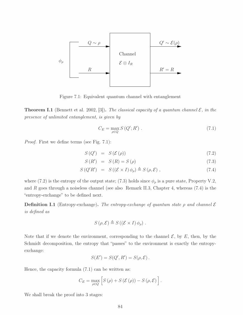
Channel

E ⊗ IR

Q ∼ ρ

R

Q′ ∼ E(ρ)

R′ = R

φρ

Figure 7.1: Equivalent quantum channel with entanglement

Theorem I.1 (Bennett et al. 2002, [3]). The classical capacity of a quantum channel E , in the

presence of unlimited entanglement, is given by

CE = maxρ∈Q

S (Q′;R′) . (7.1)

Proof. First we define terms (see Fig. 7.1):

S (Q′) = S (E (ρ)) (7.2)

S (R′) = S (R) = S (ρ) (7.3)

S (Q′R′) = S ((E × I)φρ) , S (ρ, E) , (7.4)

where (7.2) is the entropy of the output state; (7.3) holds since φρ is a pure state, Property V.2,

and R goes through a noiseless channel (see also Remark II.3, Chapter 4, whereas (7.4) is the

“entropy-exchange” to be defined next.

Definition I.1 (Entropy-exchange). The entropy-exchange of quantum state ρ and channel Eis defined as

S (ρ, E) , S ((E × I)φρ) .

Note that if we denote the environment, corresponding to the channel E , by E, then, by the

Schmidt decomposition, the entropy that “passes” to the environment is exactly the entropy-

exchange:

S(E ′) = S(Q′, R′) = S(ρ, E) .

Hence, the capacity formula (7.1) can be written as:

CE = maxρ∈Q

[S (ρ) + S (E (ρ)) − S (ρ, E)

].

We shall break the proof into 3 stages:

84

1. Acheiving the rate S (ρ) + S (E (ρ)) − S (ρ, E) for ρ = Id, where d = dimQ.

2. Generalization for ρ = Ptr(P )

, for some projection matrix P .

3. Generalization for all ρ.

Stage 1: ρ = Id.

Generalization of superdense coding to general dimension:

Transmitter and receiver share state∣∣ψAB

⟩such that d = dimA = dimB and trA

∣∣ψAB⟩ ⟨ψAB

∣∣ =

I/d, where A denotes the transmitter system and B - the system of the receiver.

Remark I.1. The state |ψAB〉〈ψAB| is maximally entangled, as ρ ≡ ρA = Id, similarly to the

Bell state, see Section VII, Chapter 2.

By Theorem II.1, Chapter 4 (Schmidt decomposition) we can decompose |ψAB〉 as

∣∣ψAB⟩

=1√d

d∑

j=1

|jA〉 |jB〉

with |jA〉, |jB〉 being some orthonormal bases of A,B respectively. Applying a unitary

operator U to A gives rise to the state

(U ⊗ I)∣∣ψAB

⟩=

1√d

d∑

j=1

U |jA〉 |jB〉 ,

which is also maximally entangled, as local unitary operations cannot change the r.d.m..

In superdense coding for d = 2 we were able to produce 4 orthogonal states, i.e., an orthonormal

basis of AB, using local unitary operators (Pauli matrices), applied to system A only. This

can be generalized to any (natural) d: it is possible show there exists a set of d2 local unitary

operators Uid2

i=1 of A, such that(Ui ⊗ I)

∣∣ψAB⟩d2

i=1constitutes an orthonormal basis of AB.

Corollary 7.1. If a clean (“noiseless”) channel exists between transmitter and receiver, then

using SDC of dimension d, i.e., to transmit 2 log d classical bits (cbits) using a system of

dimension d.

For the noisy channel, we shall use∣∣ψAB

⟩and take d = dimQ.

We may think of∣∣ψAB

⟩as a state that was created at the transmitter, where B passes through

a clean channel. Hence

CE (E) ≥ C ′ (E ⊗ I) ≥ C ′CQ (E ⊗ I) ,

85

where C ′ and C ′CQ stand for the “regular” capacities, i.e., without entanglement, subject to a

constraint of an input ensemble of the form|ψi〉 = (Ui ⊗ I)

∣∣ψAB⟩

, where the subsystem A

is transmitted through the channel E , and the subsystem B is a fixed state at the transmitter

which passes through a clean channel I. Hence, we choose an input ensemble of the form:ψABi

,(Ui ⊗ I)

∣∣ψAB⟩d2

i=1, with equal probabilities pi = 1

d2, where |ψAB〉 is some fixed

maximally entangled state.

The mixes input state is, therefore,

d2∑

i=1

1

d2

(Ui ⊗ I

) ∣∣ψAB⟩ ⟨ψAB

∣∣(U †i ⊗ I

)=Id2

d2=Idd

⊗ Idd

= ρ⊗ ρ

, and the output state is

(E ⊗ I)

(I

d⊗ I

d

)= E (ρ) ⊗ ρ .

To find the output state given an input state (or equivalently i), note that each input state

ψi = (Ui ⊗ I)ψψAB is a purification of I/d, and hence, according to Property V.2, Chapter 4:

ρ = trB((Ui ⊗ I)

∣∣ψAB⟩)

=I

d= ρ .

Hence the output state given i may be written as (E ⊗ I)φiρ, with φiρ(≡ ψi), being a purification

of ρ = Id.

Remark I.2. S((E ⊗ I)φiρ

)does not depend on the exact purification, and hence is constant

for all i.

Combining all the results above, we arrive at

CE (E) ≥ C ′CQ (E ⊗ I) ≥ S (E (ρ) ⊗ ρ) − 1

d2

∑

i

S((E ⊗ I)φiρ

)

= S (E (ρ)) + S (ρ) − S ((E ⊗ I)φρ)︸︷︷︸S(ρ,E)

,

where the second inequality is true for our choice of the ensemble and the equality is due to

Remark I.2.

Stage 2: ρ = Ptr(P )

, for some projection matrix P .

If we limit the input to the subspace spanned by P , of dimension d′ = tr(P ), we get an effective

channel E ′. The proof of first step then applies, by taking the input to be ρ′ = Id′

.

Stage 3: generalization to any ρ.

Denote by Pn the projection operator on the typical subspace of ρ⊗n, and define the state

Πn = Pntr(Pn)

. We shall use Πn, as it is asymptotically equal to ρ⊗n, and therefore dimΠn ≈ 2nS(ρ).

86

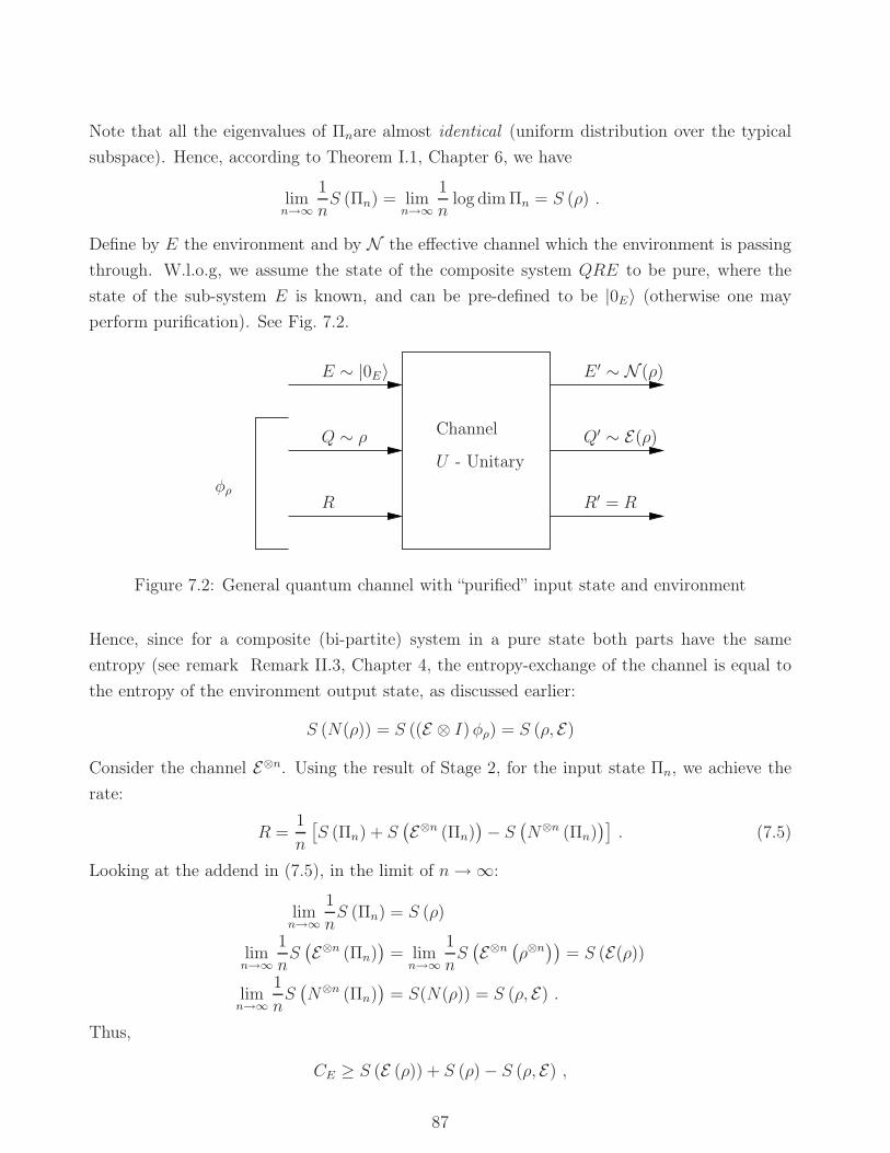
Note that all the eigenvalues of Πnare almost identical (uniform distribution over the typical

subspace). Hence, according to Theorem I.1, Chapter 6, we have

limn→∞

1

nS (Πn) = lim

n→∞

1

nlog dim Πn = S (ρ) .

Define by E the environment and by N the effective channel which the environment is passing

through. W.l.o.g, we assume the state of the composite system QRE to be pure, where the

state of the sub-system E is known, and can be pre-defined to be |0E〉 (otherwise one may

perform purification). See Fig. 7.2.

Channel

U - Unitary

Q ∼ ρ

R

Q′ ∼ E(ρ)

R′ = Rφρ

E ∼ |0E〉 E ′ ∼ N (ρ)

Figure 7.2: General quantum channel with “purified” input state and environment

Hence, since for a composite (bi-partite) system in a pure state both parts have the same

entropy (see remark Remark II.3, Chapter 4, the entropy-exchange of the channel is equal to

the entropy of the environment output state, as discussed earlier:

S (N(ρ)) = S ((E ⊗ I)φρ) = S (ρ, E)

Consider the channel E⊗n. Using the result of Stage 2, for the input state Πn, we achieve the

rate:

R =1

n

[S (Πn) + S

(E⊗n (Πn)

)− S

(N⊗n (Πn)

)]. (7.5)

Looking at the addend in (7.5), in the limit of n→ ∞:

limn→∞

1

nS (Πn) = S (ρ)

limn→∞

1

nS(E⊗n (Πn)

)= lim

n→∞

1

nS(E⊗n

(ρ⊗n))

= S (E(ρ))

limn→∞

1

nS(N⊗n (Πn)

)= S(N(ρ)) = S (ρ, E) .

Thus,

CE ≥ S (E (ρ)) + S (ρ) − S (ρ, E) ,

87

for any admissible ρ, or equivalently

CE ≥ maxρ∈Q

S (E (ρ)) + S (ρ) − S (ρ, E) .

The converse stems from a similar construction using the connections between CE and CCQ,

given in Section I.1, and from the additivity of CE mentioned below.

Remark I.3.

• For classical channels, entanglement obviously cannot increase capacity, i.e., CE = C.

• CE (E1 ⊗ E2) = CE (E1) + CE (E2).

• The entanglement-assisted capacity of the depolarizing channel, defined in Example I.1,

Chapter 6, is CE = 2−H(1 − 3

4p, 1

4p, 1

4p, 1

4p), achieved by ρ = I

2, which is strictly greater

than C = 1 − hb(p2

)for p > 0. See also Fig. I.3.

0 0.2 0.4 0.6 0.8 10

0.2

0.4

0.6

0.8

1

1.2

1.4

1.6

1.8

2

p

R [b

its]

C

E

C

Figure 7.3: Capacity and entanglement-assisted capacity of the depolarizing channel

• The entanglement-assisted capacity of the erasure channel, defined in Example I.3, Chap-

ter 6, is CE = 2(1 − p) = 2C. Superdense coding turns the channel into two parallel

quantum erasure channels (with no entangelement).

• Cost of protocol [13]: S (ρ) ebits (EPR pairs) per channel use suffice to achieve CE.

88

I.1 Relation between CE and CCQ

Consider the system QRE of the proof of Theorem I.1. Using the Schmidt decomposition

(Theorem II.1, Chapter 4) of φρ we can write the input state of the system as:

|ψ〉 =∑

x

√px|xR〉|xQ〉|0E〉 .

Note that S(ρ) = H (px). The output state of the system is therefore

∑

x

√px|xR〉|ψQ

′E′

x 〉 .

Having in mine the result of Theorem I.1, we evaluate S(Q′;R′).

Measuring R (or R’) according to the basis∣∣xR

⟩.

we get the mixed output state

∑

x

px|x〉〈x|R ⊗ |ψx〉〈ψx|Q′E′

.

Thus, the mutual information of interest is

S (Q′;R′) = H (px)︸︷︷︸S(R′) after measure

+ S (E (ρ))︸︷︷︸did not change,

since measurement is

unitary and local

−[H (px) +

∑pxS (E (ρx))

]

︸︷︷︸entropy-exchange

= S (E (ρ)) −∑

pxS (E (ρx)) = χ (px, ρx) ,

which is exactly CCQ.

Corollary 7.2. CCQ is achieved by measuring the system R (alone) ⇔ destruction of entan-

glement.

II Quantifying Entanglement

We have seen that ebits (EPR pairs) are very useful. Hence, we would like to be able to quantify

the amount of ebits available.

Assertion II.1 (Entanglement Distillation of Pure States). Assume Alice and Bob share n

copies of |ψ〉 and n is “large”. Define ρ = trA (|ψ〉〈ψ|). Then Alice and Bob can convert these

copies into ≈ nS (ρ) ebits using only local operations.

89

Proof. Using the Schmidt decomposition (Theorem II.1, Chapter 4) for each of the shared

states, we can rewrite the shared block as

(|ψ〉)⊗n =

(d∑

i=1

√λi∣∣iA⟩ ∣∣iB

⟩)⊗n

=∑

i1,i2,...,in

(λi1 ...λin)12

︸︷︷︸The same coeff.

for all summands

of the same type

∣∣iA1 ...iAn⟩ ∣∣iB1 ...iBn

⟩,

where λi are the eigenvalues of ρ.

Denote by Tk the kth type for some fixed enumeration. Then,

|ψ〉⊗n =∑

k

αk∑

(i1,...,in)∈Tk

∣∣iA1 ...iAn⟩ ∣∣iB1 ...iBn

⟩,

where αk , (λi1 ...λin)12 |Tk| and |Tk| is the cardinality of Tk.

Remark II.1. The analysis here is similar to the one made for quantum compression (The-

orem I.1, Chapter 3): in the quantum compression theorem proof, we were only interested in

(“weak”) typicality. Here we are interested in the exact type (“strong typicality”).

Define the following projectors:

PAk - the projectors on the subspace of Tkin system A;

PBk - the projectors on the subspace of Tkin system B.

Alice measures her state halves using the POVMPAk

, whereas Bob - using

PBk

. Alice and

Bob will measure the same type!1

The shared state, if result k (type Tk) was measured, is:

|ϕk〉 =1√|Tk|

∑

(i1,...in)∈Tk

∣∣iA1 ...iAn⟩ ∣∣iB1 ...iBn

⟩,

and its probability is pk = |αk|2 = λi1λi2 · · ·λin |Tk|2. In fact, we got this way a uniform

distribution over a subspace of dimension Tk. In case |Tk| = 2l (l ∈ N), there are 2l terms in

the Schmidt decomposition of |ϕk〉, which are in fact ebits.

If |Tk| is not a power of 2, then we can repeat the procedure for m blocks and suffer a loss

which vanishes for m→ ∞.

Corollary 7.3. Using local unitary transformation, it is possible to establish any orthogonal

basis, in particular a basis that is a product of l ebits.

1This is in fact a generalization of the EPR paradox (Section VII, Chapter 2).

90

AEP suggests,

Ek log |Tk| = nS (ρ)

n (S(ρ) − δ) ≤ logTk ≤ n (S(ρ) + δ)

w.p. 1.

Hence nS(ρ) ebits may be generated from n copies of |ψ〉, when n goes to infinity, using local

operations only.

Remark II.2.

• The operation, described in Assertion II.1, is called “entanglement distillation” and de-

noted by ED. Assertion II.1 suggests that

Ed (|ψ〉) ≥ S (ρ) .

• The reverse operation, which transforms ebits into a block of a tensor product of the same

((less entangled) ) shared state is termed “entanglement dilution”. The quantity of how

many ebits are needed, per copy of a quantum state, is called “entanglement of formation”

(denoted by EF ). It is possible to prove that, for a pure state |ψ〉:

EF (|ψ〉) ≥ S (ρ) ,

with high fidelity (which approaches 1 for n→ ∞).

This is achieved by Alice preparing the states (|ψ〉)⊗n, keeping part, compressing the other

part using ≈ nS(ρ) qubits with high fidelity, and teleporting these qubits to Bob. Of course,

classical communication is required for this protocol.

• LOCC model (local operation classical communication) Working in the LOCC framework,

and assuming a pure state |ψ〉, we have

Ed (|ψ〉) = EF (|ψ〉) = S (ρ) ,

where ρ , trA(|ψ〉〈ψ|).

• If the shared state is mixed, only bounds on Ed(ρAB

)and EF

(ρAB

)are known.

– Entanglement states exist from which it is impossible to create (“distill”) ebits, i.e.,

Ed(ρAB

)= 0 but EF

(ρAB

)> 0. This means that one can take ebits, form mixed

states out of them, and not to be able to “distill” any ebits back (“irreversible”).

91

– The “One-shot entanglement of formation” is defined as

E(1)F (ρ) = min

∑

i

piEF (|ψi〉) : ρ =∑

i

pi |ψi〉〈ψi|.

Clearly EF (ρ) ≤ E(1)F (ρ). It is not known whether

E(1)F (ρ1 ⊗ ρ2) = E

(1)F (ρ1) + E

(1)F (ρ2) ,

that is, whether it is additive or just ≤ . Nevertheless, Paz, Silva and Rains claim to

have proved this. If this indeed to be true, many other relations could be derived.

92

Chapter 8

Further Notions of Capacity

Summary by Ohad Barak.

I Operator-Sum Representation

We present an equivalent characterization of quantum operations to that of Definition I.1,

Chapter 6.

Theorem I.1 (Kraus). E(ρ) describes a quantum channel if and only if it can be written as

E(ρ) =

K∑

k=1

EkρE†k ,

where the channel operators Ek are mappings from the input Hilbert space to the output

Hilbert space,

Ek : Hdin → Hdout

and satisfy the completeness equation:

K∑

k=1

E†kEk = I (8.1)

and K, the “Completeness Rank”, satisfies

1 ≤ K ≤ dindout .

We shall not present the proof, as it is merely technical.

93

Example I.1 (Closed system). According to Postulate III, Chapter 1, the evolution of a closed

quantum system is described by some unitary operator U , i.e.,

E(ρ) = UρU † .

In this case there is a single channel operator E1 = U .

Example I.2 (Measurement). A (“generalized”) measurement on a system is described by a col-

lection of “measurement operators” Mm, which satisfy the completeness equation, as suggested

by Postulate IV, Chapter 1 and Section IV, Chapter 2:

E(ρ) =∑

m

MmρM†m .

We see that the channel operators Em are exactly the measurement operators Mm!

As indicated by Theorem III.1, Chapter 1, a measurement can be described by adding an ancilla

system, carrying a unitary operator and discarding. Theorem I.1 suggests the opposite direction

as well: a unitary operation on a system and its environment, followed by the discarding of the

environment is equivalent to a measurement.

Remark I.1.

1. The completeness requirement (8.1) is equivalent to the requirement that tr (E(ρ)) = 1.

2. The matrix representation of the operators Ek is not necessarily square (when din 6= dout).

3. Every channel can be represented by many different sets of channel operators. These sets

correspond to different choices of the basis of the environment.

4. The set of channel operators is also called a superoperator. The operators themselves are

called Kraus operators.

Theorem I.2. E(ρ) is a quantum channel if and only if all the following conditions hold:

1. tr(E(ρ)) = 1 ∀ρ.

2. For every input ensemble pi, ρi: E (∑

i piρi) =∑

i piE(ρi).

3. E is completely positive: if E operates on a system A, then for every system R we have

(E ⊗ IR) (ρAR) ≥ 0.

Remark I.2. Complete positiveness is a stronger requirement than definite positiveness.

94

Due to items 1 and 3 a quantum channel is referred to as Completely Positive Trace Preserving

mapping, commonly abbreviated CPTP.

Example I.3 (Depolarizing channel). Recall the depolarizing channel Example I.1, Chapter 6:

E(ρ) = (1 − ρ)ρ+ ρI

2.

This is not an operator-sum representation! To find the opeartor-sum representation, we shall

use the following identity, that holds for every ρ:

I =1

2[ρ+XρX + Y ρY + ZρZ] ,

where X, Y, Z are the Pauli matrices, defined in Example III.8, Chapter 1. This identity is

proved in the home assignment. Thus,

E(ρ) =

(1 − 3

4p

)ρ+

ρ

4[XρX + Y ρY + ZρZ] .

and the channel operators are, therefore

√1 − 3p

4I,

√p

2X,

√p

2Y,

√p

2Z

.

Hence, an alternative of looking on the depolarizing channel is that the channel has no effect on

the input state w.p. (1− 3p4) and activates one of the operators X, Y or Z with equal probabilities

otherwise.

Remark I.3. An equivalent representation would be

√1 − pI,

√p

3X,

√p

3Y,

√p

3Z

,

which is obtained by replacing 34P with P .

II Entanglement Fidelity

So far we discussed the fidelity between the input and output states of a quantum operation.

However, this does not tell us how well is the entanglement between the input state and its

environment is preserved by the quantum operation. Hence, F (ρ, E(ρ)) is not a suitable fidelity

measure for this case. Instead we examine the fidelity between the purification of the input

state and its corresponding output state, where the added system represents the entanglement.

95

E

R

Q ∼ ρ

R′

Q′ ∼ E(ρ)

Definition II.1 (Entanglement fidelity). The entanglement fidelity of a channel E with input

state ρ ∈ Q is defined by:

Fe(ρ, E) , F (RQ,R′Q′) = 〈RQ| [(IR ⊗ E)(|RQ〉〈RQ|)] |RQ〉 ,

where |RQ〉 is some purification of the state ρ of Q.

Property II.1.

1. 0 ≤ Fe(ρ, E) ≤ 1. Furthermore, Fe(ρ, E) = 1 if and only if

E(|ψ〉〈ψ|) = |ψ〉〈ψ| ∀ |ψ〉 ∈ supp(ρ) .

2. Fe does not depend on the purification preformed.

3. If E is described by a set of Kraus operators Ek, then

Fe(ρ, E) =∑

k

|tr(ρEk)|2 .

4. Fe(ρ, E) ≤ F (ρ, E(ρ)).

This means that entanglement fidelity is a more stringent measure than “regular” fidelity.

Thus, “good” entanglement fidelity guarantees “good” “regular” fidelity as well.

5. Concavity: Fe (∑

i piρi, E) ≤∑i piFe(ρi, E).

6. By combining 4,4 we have that for any decomposition ρ =∑

i piρi the following inequality

holds:

Fe(ρ, E) ≤∑

i

piF (ρi, E(ρi)) = F .

7. S(ρ) is still an achievable rate under entanglement fidelity criterion.

96

III Coherent Communication

Define the following systems:

A - Alice’s system (transmitter).

B - Bob’s system (receiver).

E - Eve’s system (environment).

Definition III.1 (qubit channel (noisless)). A (noiseless) qubit channel is the ability to perform

the mapping

|xA〉 −→ |xB〉|θE〉

for |x〉 ∈ |0〉, |1〉 and |θE〉 some fixed state of the environment.

A qubit (quantum bit) channel allows to convey any qubit:

α|0A〉 + β|1A〉 −→ (α|0A〉 + β|1A〉) ⊗ |θE〉 trE−→ α|0B〉 + β|1B〉 .

Definition III.2 (cbit channel (noiseless)). a cbit (classical bit) channel is the ability to per-

form the mapping

|xA〉 −→ |xB〉|xE〉 .

A cbit channel allows to convey the states |0〉, |1〉 perfectly, but not other state (superpositions

of these two states):

α|0A〉 + β|1A〉 −→ α|00BE〉 + β|11BE〉 trE−→ |α|2|0〉〈0|B + |β|2|1〉〈1|B .

That is to say that if we try to pass a qubit through this “classical” channel, we get on its output

a statistical mixture of the states |0〉, |1〉. This is equivalent to measuring the input with the

basis |0〉, |1〉 and sending the outcome over a classical channel. This phenomenon, in the

process of which quantum superposition turns into statistical mixture, is called “decoherence”.

Definition III.3 (cobit channel (noiseless)). A cobit (coherent bit) channel is the ability to

perform the mapping

|xA〉 −→ |xA〉|xB〉|θE〉 .

With a cobit channel at hand we can implement a cbit channel, but not a qubit channel (“no

cloning”). Nevertheless, a cobit channel, unlike a cbit one, allows to attain entanglement:

α|0A〉 + β|1A〉 −→(α|00〉AB + β|11〉AB

)⊗ |θE〉 trE−→ α|00〉AB + β|11〉AB .

97

Note that we can imitate a cobit channel with a qubit channel, by using a unitary operator

that satisfies:

U |0A〉|0B〉 = |0A〉|0B〉U |1A〉|0B〉 = |1A〉|1B〉 ,

or equivalently

U |xA〉|0B〉 = |xA〉|xB〉 .

Such an operator can be easily constructed, for instance:

U = |00〉〈00|+ |11〉〈10| + |01〉〈01|+ |10〉〈11| .

The aforementioned relations are summarized in the form of resource inequalities, as follows:

qubit ≥ cobit ≥ cbit (8.2)

cobit ≥ ebit (8.3)

where ‘≥’ means that the right-hand side resource can be implemented by the resource on the

other flank, but not vice versa.

III.1 Replacing Classical Operations by Coherent Opeartions

It is sometimes possible to turn classical communication into coherent communication, with or

without loss in rate. This is done by:

• Turning destructive operations like measurements into unitary operations + environment

and keeping the environment.

• Turning classically-dependent operations into quantum-dependent ones.

Example III.1. Suppose that some protocol uses a classical switch that chooses between

the quantum operations (Pauli matrices) I and X, according to the value of some cbit.

This can be turned into a quantum controlled-X gate.

Example III.2 (Superdense coding). We have seen in Section I, Chapter 2, that by using

superdense coding we have: 1qubit + 1ebit ≥ 2cbits. Turning it into a coherent protocol gives

rise to the following relation

1qubit + 1ebit ≥ 2cobits .

98

Example III.3 (Teleportation). We have seen in Section II, Chapter 2, that by using quantum

teleporatation coding we have: 2cbits+ 1ebit ≥ 1qubit. Turning it into a coherent protocol gives

rise to the following relation

2cobits + 1ebit ≥ 1qubit + 2ebits .

IV Private / Secret-Key Classical Capacity

Assume a quantum channel E from Alice to Bob.

Goal: Transmission of private information between Alice and Bob, such that a potential

eavesdropper (Eve) could recover and information of what was transmitted.

Environment is the part that Alice and Bob are ignorant of, and therefore functions as “noise”

from their point of view.

Strict Assumption: The Eavesdropper (Eve) has access to all the environment E that cor-

responds to the channel E , and can apply any quantum operation to it.

Definition IV.1 (Private communication). Private communication is the ability to convey

information of some (classical) rate R between A and B, such that asymptotically:

Iacc(E;BT ) ≡ Iacc(Environment,Message)n→∞−→ 0 ,

where BT is the transmitted system.

Example IV.1 (Coherent communication). A special case (and not equivalent) of Defini-

tion IV.1 is the ability to hold coherent communication of rate R between A and B:

|xnRA 〉 −→ |xnRA 〉|xnRB 〉|θE〉

or, in other words, to perform coherent communication with rate R from A to B.

Definition IV.2 (Private capacity). The private capacity of channel E , denoted by CP (E), is

the highest achievable private communication for this channel.

Remark IV.1. Theorem I.1 cannot be used directly here, i.e., in general Cp(E) 6= CCQ(E).

For instance, one notes that CCQ does not provide coherent communication, since the environ-

ment still depends on the message at the end of the protocol.

Let E be some quantum channel and define (see also Fig. 8.1): A - The system that stays at

the encoder throughout the whole process (Alice). This system is assumed to be in pure state

99

(since otherwise purification can be performed).

Q - The quantum system at the input to the channel, that is sent to Bob.

E - The environment of the input channel state (of Q).

B - The system at the output of the channel (Bob).

E ′ - The environment system at the output of the channel (Eve).

UE - A unitary expansion of E .

UEE

Q ∼ ρ

A

E ′ ∼ N (ρ)

B ∼ E(ρ)

Figure 8.1: Secret Key

Definition IV.3 (Coherent information). The coherent information of channel E with input ρ

is defined as the difference between the output entropy and the entropy-exchange:

Ic(ρ, E) , S(E(ρ)) − S(ρ, E) .

Definition IV.4 (Private information). The private information of channel E with input ρ is

defined as

Ip(ρ, E) , Ic(ρ, E) − minpx,ρx

∑

x

pxIc(ρx, E)

∣∣∣∣∑

x

pxρx = ρ

.

Theorem IV.1 (Devetak 2005, [7]). The private classical capacity of channel E is given by

Cp(E) = limn→∞

1

nmaxρ∈H⊗n

in

Ip(ρ, E⊗n

).

Sketch of direct. We shall use the input ensemble px, ρx, ρ =∑pxρx.

The composite input system AQE is in state

∑

x

px|x〉〈x|A ⊗ ρx ⊗ |0〉〈0|E .

The composite output system is in state

∑

x

px|x〉〈x|A ⊗ φBE′

x ,

100

where,

trE′(φBE′

x ) = E(ρx) ,

is the channel from Alice to Bob, and

trB(φBE′

x ) = N (ρx) ,

is the channel from Alice to Eve.

According to Theorem I.1, Chapter 6, the rate

χ (E , px, ρx) = S(E(ρ)) −∑

pxS(E(ρx)) ,

is achievable. Moreover, according to (5.7), we have

S(A;B) = χ (E , px, ρx) .

Applying the same arguments to the “channel” N from Alice to Eve, we have:

S(A;E ′) = S(N (ρ)) −∑

pxS(N (ρx)) ≥ 0 .

Coding scheme:

• Block-length n.

• Alice and Bob use approximately 2nS(A;B) codewords, meaning Bob may reliably decode

(with high probability) nS(A;B) bits.

• Eve can match the message to one of approximately 2nS(A;E′) distinct sets (with high

probability, i.e., to decode approx. nS(A;E ′) bits.

• This is analogous to the situation in which Eve can recover the nS(A;E ′) MSBs (with

high prob.) while having no effect or access to any knowledge of the rest. Moreover, using

random codes it can be shown that such a mapping exists.

Corollary 8.1. In order to hold private communication between Alice and Bob, information

ought to be sent only over the left n [S(A;B) − S(A;E ′)] LSBs. Thus, the following private rate

is achievable:

Cp(E) ≥ S(A;B) − S(A;E ′) =

= S(E(ρ)) − S(N (ρ)) −∑

x

px [S(E(ρx)) − S(N (ρx))] =

= S(E(ρ)) − S(ρ, E) −∑

x

px [S(E(ρx)) − S(ρx, E)] ,

where S(N (ρ)) = S(ρ, E) is the entropy-exchange of Definition I.1, Chapter 7.

101

Finally taking the limit of n→ ∞, we achieve the desired rate.

The converse will not be given here.

Remark IV.2.

1. One can show that: Ip(ρ, E) ≥ Ic(ρ, E). Equality holds, for instance, when all ρxare pure, i.e., ρx = |ψx〉〈ψx|A: w.l.o.g. the state of the environment (Eve) can be

assumed to be some constant pure state |0E〉. Thus the received joint state of Bob and

Eve can be written as: |φSB〉 = UE |ψAx 〉|0E〉, where UE is a unitary operator, as described

by Theorem III.1, Chapter 1. Hence, this joint state is pure as well and thus the entropies

of its reduced density matrices are equal: S(E(ρx)) = S(N (ρx)).

There are examples for which Ip > Ic > 0, but it is not known whether there is a finite

gap between the two informations under maximization, in the limit of n→ ∞.

2. Ip and Ip may take negative values, but not under maximization over ρ, since for ρ =

ρx = I/din, they are equal to 0, as is the case for the choice ρ = ρx = |ψ〉〈ψ|, i.e., some

pure state, as explained in Property V.1.

3. Similarly to the definition of private communication, one can consider the problem of

private/secret-key distribution.

Definition IV.5 (Secret-key capacity). The secret-key capacity, denote by K(E), is the

maximal rate of common “key” generation, between Alice and Bob, where all communica-

tion held between the two is via a quantum channel E , such that Eve cannot attain any

information of this key sequence.

It is evident that K(E) ≥ Cp(E), since Alice can simply choose a random sequence in

an i.i.d. manner according to Ber(1/2) and send it, using the private communication

scheme. However, one could suggest that since the exact key sequence is not interesting

as long as it is random, known to both Alice and Bob and no information of it can be

recovered by Eve, the secret-key capacity may be strictly larger than the private capacity,

at least for some channels. Nonetheless, it turns out that

K(E) = Cp(E)

for all quantum channels E .

4. The presence of a classical infinite-capacity public channel from Alice to Bob cannot

increase Cp(E) or K(E).

5. It is possible to perform the private communication protocol absolutely coherently only for

ensembles for which Ip = Ic, for instance, ensembles of pure states.

102

V Entanglement-Generating Capacity

Definition V.1 (Entanglement-generating capacity). The Entanglement-generating capacity of

a quantum channel E , denoted by E(E), is the maximal possible rate of generating EPR pairs,

shared by the transmitter and receiver.

Theorem V.1. The Entanglement-generating capacity is upper bounded by the secret-key and

private capacities:

E(E) ≤ K(E) = Cp(E) .

Proof. We shall prove that the secret-key capacity upper bounds the entanglement-generating

capacity. Out of every ebit, shared by Alice and Bob, they can produce a random bit, using

local measurements with respect to the Schmidt basis, as explained in the proof of Theorem I.1.

The resulting bits are independent of any information that could be gained by the environment

(Eve), since the ebits cannot have and (quantum or classical) dependency on the environment,

or else we would get a mixed-state, instead of a pure one, in the joint system of Alice and

Bob.

Theorem V.2. The entanglement-generating capacity is given by

E(E) = limn→∞

1

nmax

ρ∈Hin⊗nIc(ρ, E⊗n) .

Proof. The converse stems from Theorem V.1. For the achievability we consider the coherent

key generation protocol, which is possible for Ip = Ic, as suggested by Remark IV.2. Hence,

using Theorem IV.1, we may convey cobits with rate Ic. Now, using (8.3), we achieve the

desired result.

Property V.1 (Ic, S(ρ, E)).

• W.l.o.g., we take system E to be a purification of AQ, viz., the state of the joint system

AQE is some pure state |AQE〉. Thus the input state of the composite system AQE

is pure, as is the output state |ABE ′〉, since it is merely the state |AQE〉 after passing

through the unitary operation IA ⊗ UQEE .

• Since |ABE ′〉 is a pure state, S(E ′) = S(AB), according to Property V.2, Chapter 4.

Thus,

Ic(ρ, E) , S(E(ρ)) − S(N (ρ)) = S(B) − S(E ′) = S(B) − S(AB) = −S(A|B) .

103

• As mentiond in Remark IV.2, Ic may indeed be negative. However, E(E) ≥ 0, since for

the choice ρ = |ψ〉〈ψ| we always have Ic(|ψ〉〈ψ|, E) = 0, since for this choice QE and thus

also BE ′ are in pure states, and hence

S(B) = S(E ′) ⇔ Ic(ρ, E) = S(B) − S(E ′) = 0 .

• The following notation is often used:

Ic(ρ, E) ≡ Ic(A > B) .

Note that, in general, I(A > B) 6= I(B > A).

• The coherent information obeys a data processing inequality, as suggested by the following

theorem.

Theorem V.3 (Quantum data processing inequality). Let E1 and E2 be some two quantum

channels and ρ some quantum state. Then

S(ρ) ≥ Ic(ρ, E1) ≥ Ic(ρ, E1 E2) ,

with equality iff it is possible to perfectly reverse the operation E1, i.e., iff there exists a

quantum operation R such that Fe(ρ,R E1) = 1.

This is one of the reasons that for a long time Ic was “suspected” to be the quantum

channel capacity, which turned out to be true, see Theorem VI.1.

• The entropy-exchange S(ρ, E) satisfies the quantum Fano inequality.

Theorem V.4 (Quantum Fano inequality). Let ρ be a quantum state and E a quantum

channel. Then

S(ρ, E) ≤ hb(Fe(ρ, E)) + (1 − Fe(ρ, E)) log(d2 − 1) ,

where d is the dimension of the input space, and hb(•) is the binary entropy.

Thus in order to get high fidelity the entropy exchange ought to be low.

• Unfortunately, the maximum over the coherent information Ic is not additive. Thus in

general, we may not remove the "lim" in Theorem V.2.

• The entropy-exchange S(ρ, E), can be expressed as a VN entropy of a state W , where W

depends on ρ and the Kraus operators of E , in the following way:

Wij , tr(EiρEj†) ,

S(ρ, E) ≡ S(W ) , −tr(W logW ) .

104

VI The Quantum Channel Capacity

Define the following quantum channel and coding scheme:

n - coding block-length.

H - Hilbert space of the information source (increases with n).

Hin - channel input Hilbert space.

Hout - channel output Hilbert space.

E - quantum channel (CPTP); E : ∆(Hin) → ∆(Hout).

E - encoder (CPTP); E : ∆(H) → ∆(H⊗nin

).

D - decoder (CPTP); D : ∆(H⊗nout

)→ ∆(H).

The fidelity of the encoding scheme is given by

F = min|ψ〉∈H

F (|ψ〉, (D E⊗n E)(|ψ〉〈ψ|)) .

Definition VI.1 (Achievable quantum rate). A rate

R =1

nlog dimH

[qubits

channel use

],

is said to be achievable if there exists a sequence of coding schemes such that the fidelity F tends

to 1 as n→ ∞.

Definition VI.2 (Quantum capacity). The quantum capacity of a quantum channel E , denoted

by Q(E), is the supremum over all achievable rates of this channel.

Definition VI.3 (Quantum capacity (alternative definition)). Define the fidelity of the channel

E as F (ρ) = Fe(ρ,D E⊗n E) and the rate of the scheme as R = S(ρ). Then the quantum

channel capacity, Q(E), is the supremum of all achievable rates, where optimization is done

over over all admissible d.m. ρ and D and E.

Remark VI.1. Definition VI.2 and Definition VI.3 are equivalent capacity-wise [2].

Definition VI.4 (Entanglement-assisted quantum capacity). The Entanglement-assisted quan-

tum capacity is defined as the quantum capacity in the presence of unlimited entanglement, and

is denoted by QE(E).

Assertion VI.1. The quantum capacity of a channel E is upper-bounded by its classical capac-

ity: Q(E) ≤ C(E) ≤ CE(E).

Proof. The second inequality is trivial as the use of entanglement can only increase classical

capacity. The first inequality follows from (8.2), since we can transmit 1 cbit using a single

qubit.

105

Assertion VI.2. In the presence of (unlimited) entanglement, the quantum capacity is equal

to half the classical capacity of this channel:

QE(E) =1

2CE(E) .

Proof. Achievability: Perform quantum teleportation (see Section II, Chapter 2). Hence, ac-

cording to (2.2), we have 2cbits + 1ebit ≥ 1qubit.

Converse: Perform Superdense coding (see Section I, Chapter 2). Hence, according to (2.1), we

have 1qubit+ 1ebit ≥ 2cbits.

Thus we establish the equality, in the presence of entanglement:

1qubit1ebit 2cbits .

Which concludes the proof.

Assertion VI.3. The quantum capacity of the erasure channel (see Example I.3, Chapter 6)

is Q = max(1 − 2p, 0).

Proof. To prove that we first show that for p = 0.5 the quantum capacity is Q = 0: Define

a composite channel from Alice to Bob and Charley, which is composed of erasure channels

with p = 0.5 to Bob and Charley, such that whenever an erasure occurs at Bob’s side, Charley

receivers the qubit sent by Alice with fidelity 1 and vice versa. If the capacity of the erasure

channel with p = 0.5 were strictly positive, then cloning could be performed, as both Bob and

Charley would be able to recover the same state, in contradiction to Theorem III.1, Chapter 2.

Hence the quantum capacity of the erasure channel with p = 0.5 is Q = 0.

An erasure channel with p < 0.5 can be “simulated” by time-sharing between a clean channel

(with capacity equal to 1qubit) and an erasure channel with q = 0.5 above channel. Therefore,

the weighted average of the capacities of the aforementioned channels 1 − 2p, is achievable.

The converse, i.e., that no rate larger than 1 − 2p, is proved in the home assignment. See

also Example VI.2.

Theorem VI.1 (Devetak 2005, [7]; Bennett et al. 2002, [3]). The quantum channel capacity

is given by

Q(E) = E(E) = limn→∞

1

nmaxρ∈H⊗n

in

Ic(ρ, E⊗n) .

To prove this theorem we define three more quantum capacities of channels in the presence of

different classical channel resources.

106

Definition VI.5 (Feedforward quantum capacity). The feedforward quantum capacity of a

quantum channel E , denoted by Q→(E), is the supremum over all achievable rates of this channel

in the presence of an unlimited classical channel from the transmitter to the receiver.

Definition VI.6 (Feedback quantum capacity). The feedback quantum capacity of a quantum

channel E , denoted by Q←(E), is the supremum over all achievable rates of this channel in the

presence of an unlimited classical channel from the receiver to the transmitter.

Definition VI.7 (Classically assisted quantum capacity). The classically assisted quantum

capacity of a quantum channel E , denoted by Q↔(E) or Q2, is the supremum over all achievable

rates of this channel in the presence of an unlimited bidirectional classical channel, i.e., both a

channel from the transmitter to the receiver and a channel from the receiver to the transmitter.

Definition VI.8 (Feedforward entanglement-generating capacity). The feedforward entanglement-

generating capacity of a quantum channel E , denoted by E→(E), is the maximal possible rate of

generating EPR pairs, shared by the transmitter and receiver, in the presence of un unlimited

classical channel from the transmitter to the receiver.

Remark VI.2. The feedback and classical assisted entanglement-generating capacity can be

defined in a similar manner.

Proof. Converse: Combining the results of (8.2) (8.3), we see that 1qubit ≥ 1ebit. Thus,

Q(E) ≤ E(E).

Achievability: We break the achievability proof into two stages.

Stage 1: We show that E(E) ≤ Q→(E).

A presence of a classical channel between transmitter and receiver can only increase the

entanglement-generating capacity of this channel. Thus E(E) ≤ E→(E).

But having generated E→(E) ebits per channel use, we may perform quantum teleportation of

E→(E) qubits (with fidelity 1), by making use of the classical channel available. Thus

E(E) ≤ E→(E) ≤ Q→(E) .

Stage 2: We show (not rigourously) that Q→(E) = Q(E), for any CPTP E , i.e., that the

presence of a forward classical channel (alone) does not increase quantum capacity.

The most general protocol for conveying qubits is the following:

• Alice chooses one one of the encoders Ek according to some strategy (for instance,

randomly w.p.t. some measurement result), when k can be random.

107

• Alice conveys the value of k to Bob over the classical channel and the encoded state over

the quantum channel.

• Bob opearstes with the decoder Dk.

We need this scheme to have a good fidelity. Thus, to achieve a certain rate R, we need the

following to be satisfied: for every ǫ > 0 there exist n, Dk, Ek such that

Ek

min|ψ〉

F (|ψ〉, Dk E⊗n Ek(|ψ〉〈ψ|)

≥ 1 − ǫ .

Note that k cannot depend on |ψ〉 (at least not in the limit of n → ∞), since otherwise it

would mean applying a "destructive measurement" of the state to be transmitted, which would

prevent its perfect reconstruction at the decoder (F → 1).

Therefore, there exists some k = j, which does not depend on |ψ〉, such that

min|ψ〉

F (|ψ〉, Dj E⊗n Ej(|ψ〉〈ψ|)) ≥ 1 − ǫ .

Thus, using Ej and Dj , we obtain the same rates without the need of any classical communi-

cation, meaning:

Q→(E) = Q(E) .

Example VI.1 (Depolarizing channel). An explicit expression for the quantum capacity of the

depolarizing channel (see Example I.1, Chapter 6) is not known in general. Nevetheless, it is

lower bounded by

Q ≥ 1 − h(3

4p) − 3

4p · log2 3

meaning Q > 0 for p < 0.254.

On the other hand, it can be shown that Q = 0 for p > 1/3.

Example VI.2 (Erasure channel). The choice ρ = I2n

, achieves capacity asymptotically:

Q == limn→∞

1

nIC

(I

2n, E⊗n

)= max(1 − 2p, 0) .

VI.1 Classically Assisted Quantum Capacity

As was shown in the proof of Theorem VI.1, classical feedforward does not increase quantum

capacity. Nevertheless classical feedback, all the more so bidirectional classical communication,

can increase quantum capacity, as shown in the following example.

108

Example VI.3 (Feedback quantum capacity of erasure channel). The feedback quantum ca-

pacity of the erasure channel is equal to its classical capacity:

Q↔ = 1 − p = C ,

as is proved in the home assignment. Note that this is strictly larger than the its quantum

capacity (without any classical assistance), which is equal to Q = 1 − 2p < 1 − p = Q↔.

Remark VI.3. There are examples of channels for which Q < Q↔ < C.

Open Question: Is there a quantum channel for which Q↔ > C?

Open Question: TO find expressions for Q↔ and Q←.

The Example from the Beginning of the Semester

Recall Example I.1, Chapter 1.

Proposition VI.1. There are quantum channels E for which Q(E), while the quantum bidi-

rectional system, consisting of a channel E for each side (see Fig. VI.1) has a positive capacity

for quantum information.

E

EAlice Bob

Sketch. Assume a non-fixed mapping (CPTP) E , i.e., that does not map all admissible states

to the same d.m.. The classical capacity of such a channel is strictly positive, according to Re-

mark 6.1, Chapter 6. We further assume that Q↔(E) > 0. This is possible, as demonstrated

by Example VI.3 (even if Q(E) = 0).

Since C(E) > 0, we can use both channels for classical information exchange to obtain some

(striclty positive) portion of Q↔(E). Thus a strictly positive rate of quantum communication

is achievable using this system.

This protocol can be materialized using the following protocol.

109

1. Alice prepares n copies of some state ρAB.

2. Alice transmits the B parts to Bob over the channel E .

3. Alice and Bob share n copies of the state σAB = (I ⊗ E)ρAB.

4. Assuming that Ed(σAB) > 0 (true for at least some state since E is non-fixed), Alice and

Bob can prepare nEd(σAB) ebits out of many copies of σAB, working under the LOCC

model (see Section II, Chapter 7).

5. Alice and Bob perform quantum teleportation (Section II, Chapter 2), using the distilled

ebits and the classical communication.

110

Bibliography

[1] H. Barnum, C. A. Fuchs, R. Josza, and B. Schumacher. General fidelity limit for quantum

channels. Phys. Rev. A, 54:4707, 1996.

[2] H. Barnum and E. Knill M. A. Nielsen. On quantum fidelities and channel capacities.

IEEE Trans. Information Theory, IT-46:1317–1329, July 2000.

[3] C. H. Bennett, P. W. Shor J. A. Smolin, and A. V. Thapliyal. Entanglement-assisted

capacity of a quantum channel and the reverse Shannon theorem. IEEE Trans. Information

Theory, IT-48:2637–2655, Oct. 2002.

[4] T. M. Cover and J. A. Thomas. Elements of Information Theory. Wiley, New York, 1991.

[5] E. Davies. Reversing quantum dynamics with near-optimal quantum and classical fidelity.

Journal of Mathematical Physics, vol. 43:2097–2106, May 2002.

[6] E. Davies. Information and quantum measurement. IEEE Trans. Information Theory,

IT-24:596–599, Sep. 1978.

[7] I. Devetak. The private classical capacity and quantum capacity of a quantum channel.

IEEE Trans. Information Theory, IT-51:44–55, 2005.

[8] C. Fuchs. Nonorthogonal quantum states maximize classical information capacity. Phys.

Rev. Lett., 79:1162–1165, 1997.

[9] P. Hayden, R. Jozsa, D. Petz, and A. Winter. Structure of states which satisfy strong

subadditivity of quantum entropy with equality. Communications in Mathematical Physics,

vol. 246, num. 2:359–374, Feb. 2004.

[10] A. S. Holevo. Statistical problems in quantum physics. In Proc. of the Second Japan-USSR

Symposium on Probability Theory, Springer-Verlag, Berlin, 1973.

[11] M. A. Nielsen and I. J. Chuang. Quantum Computation and Quantum Information. Cam-

bridge Univ. Press, Cambridge, 2000.

111

[12] B. Schumacher. Quantum coding. Phys. Rev. A, 51:2738–2747, 1995.

[13] P. W. Shor. The classical capacity achievable by a quantum channel assisted by limited

entanglement. pages 2637–2655, submitted, 2004.

112

a course in quantum information theory

Documents