a brief course of quantum theory

A Brief Course of Quantum Theory

DONG-SHENG WANG

October 20, 2019

Contents

1 Qubits 91.1 Bit, pbit . . . . . . . . . . . . . . . . . . . . . . . . . . . . . . . . 91.2 Qubit . . . . . . . . . . . . . . . . . . . . . . . . . . . . . . . . . 101.3 Unitary evolution . . . . . . . . . . . . . . . . . . . . . . . . . . . 11

1.3.1 Rabi oscillation . . . . . . . . . . . . . . . . . . . . . . . . 121.3.2 Periodic Hamiltonian . . . . . . . . . . . . . . . . . . . . . 121.3.3 Parameter-dependent Hamiltonian . . . . . . . . . . . . . . 131.3.4 Quantum control . . . . . . . . . . . . . . . . . . . . . . . 16

1.4 Non-unitary evolution . . . . . . . . . . . . . . . . . . . . . . . . . 181.4.1 Quantum channels . . . . . . . . . . . . . . . . . . . . . . 181.4.2 Thermodynamics . . . . . . . . . . . . . . . . . . . . . . . 21

1.5 Observable and Measurement . . . . . . . . . . . . . . . . . . . . . 221.5.1 Projective measurement . . . . . . . . . . . . . . . . . . . 231.5.2 Non-commuting set of observable . . . . . . . . . . . . . . 241.5.3 Tomography, Estimation, Discrimination . . . . . . . . . . 25

1.6 The power of qubit . . . . . . . . . . . . . . . . . . . . . . . . . . 271.6.1 Black-box encoding . . . . . . . . . . . . . . . . . . . . . 271.6.2 Quantum key distribution . . . . . . . . . . . . . . . . . . . 281.6.3 Measure classical values . . . . . . . . . . . . . . . . . . . 291.6.4 Leggett–Garg inequalities . . . . . . . . . . . . . . . . . . 301.6.5 Contextuality . . . . . . . . . . . . . . . . . . . . . . . . . 31

1.7 Zoo of qubits . . . . . . . . . . . . . . . . . . . . . . . . . . . . . 32

2 Basic Formalism 352.1 Hilbert space . . . . . . . . . . . . . . . . . . . . . . . . . . . . . 35

2.1.1 States . . . . . . . . . . . . . . . . . . . . . . . . . . . . . 362.1.2 Norm . . . . . . . . . . . . . . . . . . . . . . . . . . . . . 402.1.3 Dynamics . . . . . . . . . . . . . . . . . . . . . . . . . . . 412.1.4 Measurement . . . . . . . . . . . . . . . . . . . . . . . . . 43

2.2 Quantum notions . . . . . . . . . . . . . . . . . . . . . . . . . . . 462.2.1 Information and entropy . . . . . . . . . . . . . . . . . . . 462.2.2 Entanglement . . . . . . . . . . . . . . . . . . . . . . . . . 48

i

ii CONTENTS

2.2.3 Uncertainty . . . . . . . . . . . . . . . . . . . . . . . . . . 492.3 Geometric phases . . . . . . . . . . . . . . . . . . . . . . . . . . . 51

2.3.1 Aharonov-Anandan phase . . . . . . . . . . . . . . . . . . 512.3.2 Applications . . . . . . . . . . . . . . . . . . . . . . . . . 522.3.3 Generalizations . . . . . . . . . . . . . . . . . . . . . . . . 53

2.4 Quantum channels . . . . . . . . . . . . . . . . . . . . . . . . . . 542.4.1 Representations . . . . . . . . . . . . . . . . . . . . . . . . 542.4.2 Lindblad equation . . . . . . . . . . . . . . . . . . . . . . 592.4.3 Markovianity . . . . . . . . . . . . . . . . . . . . . . . . . 602.4.4 Beyond . . . . . . . . . . . . . . . . . . . . . . . . . . . . 63

2.5 Matrix product states . . . . . . . . . . . . . . . . . . . . . . . . . 642.5.1 MPS circuit . . . . . . . . . . . . . . . . . . . . . . . . . . 662.5.2 Avoid the final projection . . . . . . . . . . . . . . . . . . . 672.5.3 Composition . . . . . . . . . . . . . . . . . . . . . . . . . 692.5.4 Extract the edge state . . . . . . . . . . . . . . . . . . . . . 702.5.5 Area law . . . . . . . . . . . . . . . . . . . . . . . . . . . 70

3 Advanced Formalism 733.1 Phase space and quantization . . . . . . . . . . . . . . . . . . . . . 73

3.1.1 Hamiltonization . . . . . . . . . . . . . . . . . . . . . . . 743.1.2 Wigner function . . . . . . . . . . . . . . . . . . . . . . . 763.1.3 Quantization . . . . . . . . . . . . . . . . . . . . . . . . . 78

3.2 Relativistic subtheory . . . . . . . . . . . . . . . . . . . . . . . . . 813.2.1 Special Relativity . . . . . . . . . . . . . . . . . . . . . . . 813.2.2 Relativistic equations . . . . . . . . . . . . . . . . . . . . . 84

3.3 Semi-classical subtheory . . . . . . . . . . . . . . . . . . . . . . . 883.3.1 Bohmian mechanics . . . . . . . . . . . . . . . . . . . . . 893.3.2 Path integral . . . . . . . . . . . . . . . . . . . . . . . . . 913.3.3 Stabilizer formalism . . . . . . . . . . . . . . . . . . . . . 92

3.4 Quantum field theory . . . . . . . . . . . . . . . . . . . . . . . . . 933.4.1 Bosonic and fermionic fields . . . . . . . . . . . . . . . . . 933.4.2 Topological fields . . . . . . . . . . . . . . . . . . . . . . . 973.4.3 Conformal fields . . . . . . . . . . . . . . . . . . . . . . . 99

4 Quantum Computation 1074.1 Universal computing models . . . . . . . . . . . . . . . . . . . . . 107

4.1.1 Turing machine . . . . . . . . . . . . . . . . . . . . . . . . 1084.1.2 Circuit model . . . . . . . . . . . . . . . . . . . . . . . . . 1104.1.3 Turing machine vs. circuit model . . . . . . . . . . . . . . 1114.1.4 Simulation . . . . . . . . . . . . . . . . . . . . . . . . . . 113

4.2 Quantum gate operations . . . . . . . . . . . . . . . . . . . . . . . 1164.2.1 Teleportation . . . . . . . . . . . . . . . . . . . . . . . . . 116

CONTENTS 1

4.2.2 Anyon braiding . . . . . . . . . . . . . . . . . . . . . . . . 1184.2.3 Other methods . . . . . . . . . . . . . . . . . . . . . . . . 119

4.3 Universal fault-tolerant QC . . . . . . . . . . . . . . . . . . . . . . 1194.3.1 Quantum codes . . . . . . . . . . . . . . . . . . . . . . . . 1194.3.2 Universal vs. Fault-tolerant gate set . . . . . . . . . . . . . 121

4.4 Examples of universal fault-tolerant QC . . . . . . . . . . . . . . . 1244.4.1 Topological QC via nanyons . . . . . . . . . . . . . . . . . 1254.4.2 3D gauge color codes . . . . . . . . . . . . . . . . . . . . . 1274.4.3 Triorthogonal codes . . . . . . . . . . . . . . . . . . . . . 1284.4.4 Concatenated codes . . . . . . . . . . . . . . . . . . . . . . 128

4.5 Quantum algorithms . . . . . . . . . . . . . . . . . . . . . . . . . 1294.5.1 Computational complexity . . . . . . . . . . . . . . . . . . 1324.5.2 Examples of quantum algorithms . . . . . . . . . . . . . . 133

5 Condensed Matter Physics 1375.1 Symmetry . . . . . . . . . . . . . . . . . . . . . . . . . . . . . . . 1375.2 Ising model . . . . . . . . . . . . . . . . . . . . . . . . . . . . . . 1405.3 Ising world . . . . . . . . . . . . . . . . . . . . . . . . . . . . . . 142

5.3.1 Fermionization . . . . . . . . . . . . . . . . . . . . . . . . 1425.3.2 Bosonization . . . . . . . . . . . . . . . . . . . . . . . . . 1435.3.3 Gauging . . . . . . . . . . . . . . . . . . . . . . . . . . . . 1445.3.4 Defects . . . . . . . . . . . . . . . . . . . . . . . . . . . . 1455.3.5 XXZ model . . . . . . . . . . . . . . . . . . . . . . . . . . 1465.3.6 Dimer models . . . . . . . . . . . . . . . . . . . . . . . . . 148

5.4 Topological phases . . . . . . . . . . . . . . . . . . . . . . . . . . 1505.4.1 Toric code . . . . . . . . . . . . . . . . . . . . . . . . . . . 1525.4.2 Fractional quantum Hall effect . . . . . . . . . . . . . . . . 1555.4.3 Topological insulator . . . . . . . . . . . . . . . . . . . . . 158

2 CONTENTS

Introduction

Question 1. What is ‘quanta’?

Quanta, or ‘Quantum’ is by no means a good name; however, there is no betterone. Max Planck discovered the constant h = 6.62606957(29)×10−34J · s, which istreated as the element, or ‘quanta’, of action.

What does ‘quantum’ mean? This is a primary but difficult question. Intuitively, anew constant will lead to new principle of nature, which, unfortunately, is not so clearyet, but implicitly sets the foundation of quantum theory. Here I spell my answerfirst, then I will explain more later. Quantum theory is a theory that describes thestructure of motion of objects. The structure of motion is the notion that differs frommotion, object, and structure of object. Traditionally in physics and our commonsense, motion is the movement in space and time, object is a ‘thing’ with mass orenergy, e.g., a ball, an electron, or the earth, and structure of object is the details ofthe parts of object, could be geometrical, chemical, etc.

From classical mechanics we know phase space. We can view quantum theoryas a generalization of it. It is a more powerful, complete version of phase spaceparadigm. Phase space is based on conjugate variables, such as position r and mo-mentum p, and their product is nothing but the action. With a Hamiltonian H(x, p),the Hamilton’s equation is

∂H∂x

=−p,∂H∂ p

= x. (1)

This is, furthermore, equivalent to Lagrangian version by L := xp−H and the prin-ciple of least action.

In quantum theory, conjugate variables are not numbers anymore. Instead, theyare collections of numbers, i.e., they are matrices, or, operators. The consequenceis that, conjugate operators, also called observable, cannot be measured at the sametime since they do not commute. This leads to the complementarity principle of NielsBohr, or the duality property.

Why a matrix is needed to describe a ‘thing’? Well, the short answer is, the thingis complicated. It cannot be well described by a single number or function. Let’ssee a most trivial thing: people wear clothes. He/she can wear different ones, he/shecan wear the same one in different situations, he/she can choose one depending on

3

4 CONTENTS

many factors, such as pocket, mood, etc. This complicated thing of wearing clothes,especially for females, has to be described by an exotic thing: an operator.

Question 2. What is the primary quantum equation?

In quantum physics, structure of the motion of one object, e.g., an electron, aredescribed as a complex vector |ψ〉 in Hilbert space, and the evolution is representedby one operator acting on the state changing its magnitude and phase. Suppose thedynamics of the particle is driven by a Hamiltonian H, then the quantum equation is

ih|ψ〉= H|ψ〉, (2)

with h = h/2π which appears much more unique than h itself. H is an operator, forwhich the eigenvalues are the possible energies. If the state |ψ〉 initially is expressedin the basis of the eigenstates of H, then the evolution of the state will include: theevolution of the coefficients of the eigenstates, which changes the relative populations(i.e. probabilities) and relative dynamical phases of the eigenstates, and the rotationof the eigenstates themselves which generates geometric phases. Let us name theabove equation as state equation, since it provides the possible states of the particle,the probabilities for the particle to be in the states, and also the relative phases amongthe states. The state equation is originally discovered by Erwin Schrodinger for aspecial case of particles without internal degree of freedoms (d.o.f).

Briefly, the state equation provides the structure of motion of an object. As theresult, quantum theory is a new kind of description of motion, which is different fromother theories, including classical mechanics, wave mechanics etc.

Question 3. Except |ψ〉 and H, why there are h and i?

The obvious reason for i is that it transfers the effects of Hamiltonian into a phase,and the constant h servers as the action element. In the early age of quantum physics,h is more important. However, it is clear now the quantum state |ψ〉 (and also H) ismore important.

There is a limit by h→ 0, which shall implies there is no quantum effect anymore.This is the correspondence principle of Bohr. The disappearance of h means theignorance of the structure of motion, e.g., averaging the detailed structure of motion,thus leading to classical results.

Question 4. What is the magic of quantum coherence?

By extending from numbers to operators, quantum theory brings us the mostimportant concept: quantum coherence. Please do not mix it with other notions ofcoherence that you know. Quantum coherence is the origin of all these quantum‘magic’: superposition, complementarity, uncertainty, entanglement, contextuality,duality, spin, etc.

CONTENTS 5

Quantum

expe

ctatio

nClassical

Statistical

Relativity

Field

decoherence

boostcoherencecollective

Figure 1: The quantum landscape. Quantum to classical: take average; quantum tostatistics: take partial trace; quantum to special relativity: boost coherence, spacetimequbit; quantum to quantum field: take continuous limit.

The most essential consequence of quantum coherence is that it allows quantumtheory to unify many theories. Quantum theory unifies classical mechanics, specialrelativity, statistical physics, electromagnetism, quantum field theory, and more. Itreduces to them under certain limits, as shown in Fig. 1. Besides, there are manytypes of coherence:

• coherence in field or vacuum: revealed by quantum field.

• coherence in matter: usual quantum theory, e.g. atomic theory.

• coherence between matter and light: revealed by quantum optics.

• coherence between matter and vacuum: revealed by special relativity.

Question 5. What is spin?

In quantum theory, there is a thing called ‘spin’. Spin is an inner d.o.f of a quan-tum object, or, particle. A macroscopic object many not have spin but no one provesthis. Again, ‘spin’ is a bad name. It does not mean a particle is spinning. In math,there is a group called ‘spin group’ (also ‘pin group’), making this term even moreweird. I have to say, I do not know the real physical meaning of spin. It has tobe explained by some ‘post-quantum’ theory. Elementary particles also have otherfeatures, such as charge, mass, color, weak charge etc, but spin is the most amazingone.

Spin is said to take integer or half-odd-integer values. It cannot be 1/3, say.However, this is not quite true. The observed value of spin can be any real values.The value of spin s actually determines the Hilbert space dimension d = 2s + 1.The dimension d can only be integers by definition (except some effective onessuch as for anyons). Spin s can also be zero. A profound theorem from quan-tum field theory is that particles are classified into two classes: bosons for integer

6 CONTENTS

spins, fermions for half integers. This is the spin-statistics theorem. A collection ofbosons (fermions) obey Bose-Einstein (Fermion-Dirac) statistics, as generalizationsof Boltzmann statistics.

Different spins obey slightly different state equations. Let’s see how it describesfree particles with spins.

• spin 0: Klein-Gordan equation.

• spin 1/2: Dirac equation.

• spin 1: Maxwell equation without source terms.

• higher spins: we will see these equations.

Question 6. Is quantum theory self-consistent?

The short answer is it must be. An amazing thing of quantum theory is that it isextendable, and the extended version is equivalent in a sense to the original one. Inother words, it is ‘closed’ or ‘self-consistent’. Here I show you two different kinds ofextensions. First, a quantum theory can be further quantized to a higher level. Thisis because ‘structure of motion’ can be treated as motion, and then a higher-levelstructure can be introduced. If you could do so consistently, then you can get moreand more complete understanding of the motion of an object. Second, a quantumtheory can be ‘de-quantized’ (or randomized in an ensemble), but can be treated aspart of a quantum theory again. This is the connection with statistical physics.

Question 7. How to interpret quantum theory?

What is ‘interpretation’? In brief, it is different understandings or explanations ofroughly the same phenomena (experiments) or mathematics. A theory needs inter-pretation since the mathematical symbols need meanings. Just like ‘gravity’, whichwas just a name and it took centuries for people to accept it, ‘quantum’ is also justa name. The power of quantum theory has been proven by the tremendous progressduring the last century.

There is a subject known as ‘interpretation of quantum theory’ or ‘quantum foun-dation’. Historically, this originates from confusions about some concepts, the role ofquantum theory itself in physics, and also about philosophical implications of quan-tum theory. These include the concepts of wavefuction, Hilbert space, spin, measure-ment, etc, and the relation with other theories such as ‘classical’ ones, and notionsof reality, causality, completeness, determinism, etc. Fortunately, nowadays we al-most know what quantum theory is, as described above. Quantum theory is a type ofunification theory, i.e., a more complete description of motion, that can include othertheories as special cases. Quantum state, which certainly is physical, describes thestructure (or scope) of the motion of objects.

CONTENTS 7

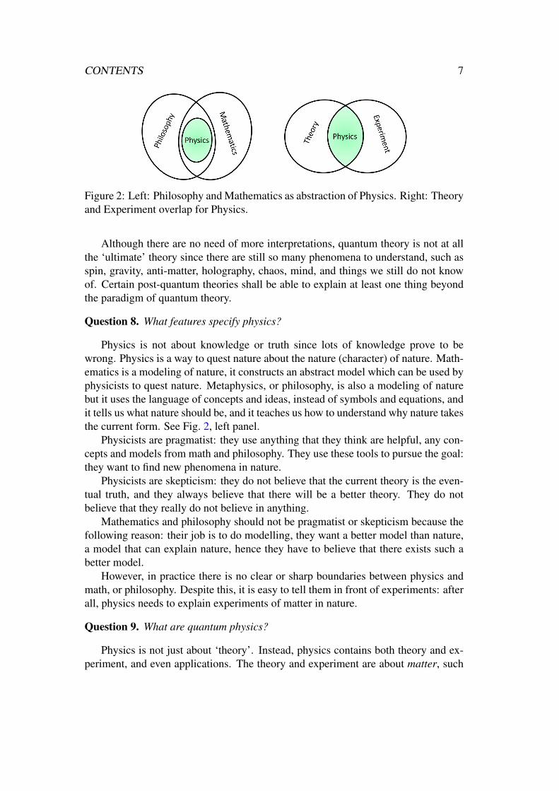
Figure 2: Left: Philosophy and Mathematics as abstraction of Physics. Right: Theoryand Experiment overlap for Physics.

Although there are no need of more interpretations, quantum theory is not at allthe ‘ultimate’ theory since there are still so many phenomena to understand, such asspin, gravity, anti-matter, holography, chaos, mind, and things we still do not knowof. Certain post-quantum theories shall be able to explain at least one thing beyondthe paradigm of quantum theory.

Question 8. What features specify physics?

Physics is not about knowledge or truth since lots of knowledge prove to bewrong. Physics is a way to quest nature about the nature (character) of nature. Math-ematics is a modeling of nature, it constructs an abstract model which can be used byphysicists to quest nature. Metaphysics, or philosophy, is also a modeling of naturebut it uses the language of concepts and ideas, instead of symbols and equations, andit tells us what nature should be, and it teaches us how to understand why nature takesthe current form. See Fig. 2, left panel.

Physicists are pragmatist: they use anything that they think are helpful, any con-cepts and models from math and philosophy. They use these tools to pursue the goal:they want to find new phenomena in nature.

Physicists are skepticism: they do not believe that the current theory is the even-tual truth, and they always believe that there will be a better theory. They do notbelieve that they really do not believe in anything.

Mathematics and philosophy should not be pragmatist or skepticism because thefollowing reason: their job is to do modelling, they want a better model than nature,a model that can explain nature, hence they have to believe that there exists such abetter model.

However, in practice there is no clear or sharp boundaries between physics andmath, or philosophy. Despite this, it is easy to tell them in front of experiments: afterall, physics needs to explain experiments of matter in nature.

Question 9. What are quantum physics?

Physics is not just about ‘theory’. Instead, physics contains both theory and ex-periment, and even applications. The theory and experiment are about matter, such

8 CONTENTS

as atom, light, liquid, solid, earth, and the universe, instead of other things, suchas people, animals, etc. However, theory and experiment only overlap to a certaindegree. A theory may have application beyond physics in other areas, such as eco-nomics, and an experiment may need theory or concepts beyond physics, such aschemistry, biology, or even computer science. See Fig. 2, right panel. So we shall beopen minded and treat physics, including quantum physics, as an open system, so itcan fit into the whole world of science and build various connections.

We shall see what quantum physicists are doing. There are many, here are some:

• atom, molecule: structure of atoms, molecules, and reactions.

• cold atom, laser: cooling atoms, interaction with laser, condensation.

• condensed matter: quantum phase transition, materials.

• high energy: elementary particles and related.

• nano: 1D, 2D, 3D structures, graphenes, semiconductors.

• optics, laser: photons, non-linearity, photonic crystal, chips.

• quantum thermodynamics: open system, heat engine.

• quantum computing: gates, channels, entanglement.

• quantum gravity: duality, black hole, universe.

• quantum chaos: few-body dynamics.

• quantum magnetism: many-body systems of spins, topological phases.

• solid-state: phonons, interaction with light, pressure, etc.

• spintronics: control of spins, magnetism, devices, logic.

• superconductors: high-temperature, junctions.

Quantum theory is becoming more and more complicated since too many thingsare squeezed into it. This brief lecture notes would not cover all topics; instead, itaims for the opposite: we try to distill the most central concepts in quantum theory,and explain them in the most simple words. Once you grasp the essence, you willfind quantum theory is amazing and you will be able to improve it.

D.-S. [email protected]: October 20, 2019

Chapter 1

Qubits

A quantum bit, or ‘qubit’, is a two-level quantum system, which is the simplest yetnontrivial quantum systems. In this chapter, we will survey many concepts and the-ories just for the case of qubit. Although there are indeed some complications whengeneralizing to other cases, we find the qubit case captures lots of the essence.

1.1 Bit, pbitA bit is an object with two states: 0 or 1. An example is a coin with a head and a tailstate. A slight generalization of bit is a probabilistic bit, or pbit, which can be at state0 or 1 with a probability. Namely, a state of a pbit can be written as p0+(1− p)1 ora vector (p,1− p) for p ∈ [0,1].

Question 10. What is the meaning of p, as probability?

This is not a new question, but we need to be careful of its physical meaning. Itis a sense of ignorance, but there are usually two types.

1. First, it is a statistical weight for a collection of identical bits. Suppose thereare N bits and there are pN of them with head state. So the state of the wholecollection can be viewed as a pbit.

2. Second, it is a dynamical abstraction for the evolution of a bit. Say, the coinis thrown N times and pN of them with head state. So the state of the wholeevent can be viewed as a pbit.

These two point of views are equivalent under a certain condition, which is knownas the ergodic condition: all points in phase space can be equally visited. Here wealready encounter the concept of phase space, which we shall study more in Chap-ter 3. In addition, there is another type that is not common in physics but somewhereelse. It is a subjective ignorance, say, due to the lack of knowledge of people. Thisrelates to Bayesian inference. However, in physics we do not deal with the lack of

9

10 CHAPTER 1. QUBITS

knowledge of people. The thing that interacts with an observed object is a physicaldevice. So p shall be explained by physical terms.

1.2 QubitA qubit is a further generalization of a pbit from real vectors to complex vectors(states). We need the Dirac notation: |ψ〉 for a state ψ . As it is complex, we use 〈ψ|for its conjugate. A qubit state can be written as

|ψ〉= α|0〉+β |1〉, α,β ∈ C, (1.1)

for |0〉 = (1,0)t , |1〉 = (0,1)t . Furthermore, we can use polar form for α and β andignore a common phase factor, then

|ψ〉= a|0〉+beiϕ |1〉, a,b,ϕ ∈ R. (1.2)

Next, we require that the state is normalized as it is in a projective Hilbert space (seeChapter 2), namely, 〈ψ|ψ〉 = 1, we have a2 + b2 = 1. So a qubit state contains tworeal parameters.

For a Hilbert space, the inner product, also known as ‘overlap’, of any two states|ψ1〉 and |ψ2〉 is defined as 〈ψ1|ψ2〉. Two states are orthogonal if their overlap is zero.For dimension d, a set of mutually orthogonal state is an orthonormal basis such thatany state can be written as a linear superposition of them. The states |0〉 and |1〉 forman orthonormal basis for a qubit.

Question 11. Is there a geometric representation of a qubit?

If we use the complex plane, then it can be viewed as two points. But this isnot so satisfactory (although this might work for qudit cases; e.g., the Majorana rep-resentation). We need to use a single point to account for two parameters. It turnsout we need a three-dimensional object, which is known as Bloch sphere, a 2-sphereembedded in R3, see Fig. 1.1.

The triangular parameters a = cosθ/2, b = sinθ/2. The factor of 2 is there sincea rotation of θ = π leads to its orthogonal state instead of itself. We then have

|ψ〉= cosθ

2|0〉+ eiϕ sin

θ

2|1〉. (1.3)

This is also known as a pure state.Mixed states, or density matrices, are those points inside the Bloch sphere, so

together they form the Bloch ball. Intuitively, a mixed state is a point whose distanceto the centre of the ball is smaller than one. How to quantify this?

Mixed states cannot be written as vectors; instead they are matrices. A mixedstate can be expanded with Pauli matrices σ i= 1,X ,Y,Z (i = 0,1,2,3) as

ρ = (1+~n ·~σ)/2, (1.4)

1.3. UNITARY EVOLUTION 11

Figure 1.1: The Bloch sphere.

with

X =

(0 11 0

),Y =

(0 −ii 0

),Z =

(1 00 −1

). (1.5)

It is trace one trρ = 1, and the purity is trρ2 = (1+ |~n|2)/2 < 1. The vector ~n isalso known as Bloch vector. For pure state, we have nx = sinθ cosφ , ny = sinθ sinφ ,nz = cosθ . For mixed state, we can denote~n = r(nx,ny,nz) for r ∈ [0,1) as the lengthof the Bloch vector. We see that a mixed qubit state contains three real parameters!

1.3 Unitary evolutionAs a matrix, a qubit state is

ρ =

(ρ00 ρ01ρ10 ρ11

). (1.6)

The diagonal elements ρ00 and ρ11 are called ‘population’ as they are the probabilityon states |0〉 and |1〉, and off-diagonal elements ρ01 and ρ10 are called ‘coherence’,and they satisfy

ρ00 +ρ11 = 1,ρ01 = ρ∗10, (1.7)

and ρ00ρ11 ≥ ρ01ρ10 due to positivity of ρ . For pure states, ρ00ρ11 = ρ01ρ10.Given a state, what shall we expect? Well, just like any object, you can apply

drives (or forces) on it to see how it evolves. This is the subject of quantum dynamicswhich studies the evolution of quantum systems. The evolution could be invertible ornot. As quantum states form Hilbert space, invertible evolution of them is describedas unitary operator U so that

U† =U−1, (1.8)

and it requires detU = 1 for simplicity.When U takes the form U = eitH , it is generated by a Hamiltonian H, which is

hermitian. The Liouville–von Neumann equation is

iρ = [H,ρ]. (1.9)


For pure states, it reduces to the state equation

i|ψ〉= H|ψ〉. (1.10)

Note we take h = 1 for simplicity.

Question 12. How to solve the above quantum equation?

The solution takes the form

|ψ(t)〉=U |ψ(0)〉 (1.11)

for an initial state |ψ(0)〉. If H can be diagonalized H = V ΛV †, for the diagonalterms of Λ known as ‘energy’, then U =VeitΛV †. Now we have encountered the firstbut most crucial problems in quantum theory: diagonalize matrices, which turn outto be very difficult in general! (and this basically motivates the subject of quantumcomputing.) However, there are enough solvable examples in physics with interestingphenomena, as discussed below.

1.3.1 Rabi oscillationFor a qubit with a diagonal Hamiltonian H, the two states are eigenstates and will ob-tain phases under free evolution. Interesting thing would happen when off-diagonalterms are added. Rabi oscillation is an example, which can describe the dynamics ofa two-level atom driven by a classical electromagnetic field.

The population of states and coherence will oscillate at Rabi frequency. Thisshows the periodic exchange of energy between the atom and the field.

What is the energy that is exchanged? They are carried by photons. The field canbe quantized as a collection of photons. The Jaynes-Cummings Hamiltonian for atwo-level atom coupled to a quantized electromagnetic field is given by

H = ω(a†a+1/2)+ω0σz/2− iΩσ

x(a−a†). (1.12)

With the rotating wave approximation (RWA), it becomes

H = ∆σz− iΩ(σ+a−σ

−a†), (1.13)

with |∆|= (ω0−ω)/2 as the detuning, σ± = (σ x±σ y)/2. The RWA ignores σ+a†

and σ−a, i.e., excite or de-excite both the spin and the field which apparently do notpreserve energy. The Rabi frequency is found by diagonalizing H to be

√∆2 +Ω2.

1.3.2 Periodic HamiltonianWhen Hamiltonian has parameter r ∈ [0,R] such that it is periodic

H(0) = H(R), (1.14)

there are interesting physical effects.


Question 13. How special can a periodic Hamiltonian be?

First, this is effectively a symmetry, denoted as G and

[G,H(r)] = 0. (1.15)

Any state ψ(r) will contain the parameter r. A common set of eigenstates ψ(r)for G and H(r) can be chosen and ψ(r+R) = λψ(r). For instance, when r is spaceposition x, G is the translation operator, R can be the lattice constant, and λ becomeseikR for Bloch wave-vector k. The interval (−π/R,π/R] is known as the Brillouinzone. The set of states ψnk(r) is known as Bloch bands. The relation betweenEn(k) and k is the dispersion relation. For a periodic Hamiltonian with time-reversalsymmetry the energy bands are degenerate between k and −k, which is the Kramersdegeneracy.

If the parameter is time t, then there is a special structure of its unitary evolution.Floquet theory shows that the time evolution operator U(t) by H(t) takes the form

U(t) = eitKV (t) (1.16)

for a hermitan operator K, a unitary operator V (t) with V (0)=1 and V (t)=V (t+T ).However, K is not easy to find. Special examples can be solved, e.g., for adiabaticevolution K can be approximated by H(t) itself.

1.3.3 Parameter-dependent HamiltonianGiven a Hamiltonian H, the spectrum is given by its eigenstates. The equationi|ψ(t)〉 = H|ψ(t)〉 can be solved. If the initial state |ψ(0)〉 is an eigenstate, thenthe evolution yields |ψ(t)〉= eiEt |ψ(0)〉 with E as the energy of |ψ(0)〉. We see thatthe dynamics only generates a phase factor eiEt .

For a time-dependent Hamiltonian, the physics becomes more interesting. First,the equation

i|ψ(t)〉= H(t)|ψ(t)〉 (1.17)

cannot be easily solved in general. Note here H(t) is not periodic. There does exist aformal solution, known as Dyson series (Chapter 2), which describes the solution asa sum of many terms, while you do not know how many terms you need to calculate,and these terms are hard to calculate. This method together with Feynman diagramis widely used in particle physics.

If the time-dependence of H(t) is of special forms, we might hope to obtainsolutions. Below we analyze an example to illustrate the idea. Consider a spin-1/2 ina magnetic field, while the field is time-dependent. The direction of B(t) is changingsmoothly. With polar coordinates, let’s consider

~B(t) = B(sinθ cosωt,sinθ sinωt,cosθ), (1.18)


i.e., the field strength B does not change, while it is rotating around the z-axis withan offset angle θ (see Fig. 1.1 but with state vector replaced by field vector). Therotation frequency ω is constant. Now, what is the form of H(t) for the spin? It takesthe form

H(t) = b~B(t) ·~S (1.19)

for the three-component spin operator ~S = (σ x,σ y,σ z). Here we ignore the detailsfor the constant b, which depends on the physical particle that carries the spin.

The model H(t) is simple enough so it can be exactly solved! First, with easyalgebra it can be written as

H(t) =V †H ′V,V := eiωtσ z,H ′ = e−iθσ y

σzeiθσ y. (1.20)

So the time-dependence is encoded in a unitary operator U which acts on a fiducialmodel H ′. Note that in general, the time-dependence of a model H(t) cannot beextracted as an external unitary operator U . Here it just happens to be the case.

Also the model we study is periodic: H(T ) = H(0) for T = 2π/ω . This meansthat the eigenvalues and eigenstates will come back to themselves after T . However,there are additional phase factors in front of each eigenstate, as we will see below.The model can be exactly solved with solution

|ψ(t)〉= e−itωσ ze−it(H(0)−ωσ z)|ψ(0)〉. (1.21)

Now we define the Aharonov-Anandan dynamical phase

αd :=

∫ T

0〈ψ(t)|H(t)|ψ(t)〉dt. (1.22)

The total phase α is defined as

e−iα := 〈ψ(T )|ψ(0)〉, (1.23)

and the geometric phase is γ := α−αd . We find that

γ = 2π(1+ω

Ω− b

Ωcosθ), (1.24)

for Ω := b√

1+ω(−2cosθ +ω/b)/b. In the limit that ω/b 1, the phase reducesto γ = 2π(1−cosθ), which is actually known as Berry’s adiabatic geometric phase.

Question 14. How good is adiabatic evolution?

The model above just happens to be exactly solvable. There are many models thatare not the case. However, as hinted above, if the evolution is adiabatic, the solutioncan also be easily handled. When the field rotates slowly in the adiabatic regime,we can use the adiabatic solution. We can denote the instaneous eigenstates as |k, t〉


with H(t)|k, t〉=E(k, t)|k, t〉. Here the energy E(k, t) are time-independent, so can besimply denoted as Ek, which is proportional to k. In this regime, if it starts on |k,0〉,the system will stay on its instaneous eigenstate |k, t〉 with the same k. There will bea tiny jump to other states, though. Given a set of instaneous eigenstates |k, t〉, thecondition for the adiabatic approximation is that

〈k, t|∂t |k′, t〉 ≈ 0, ∀k 6= k′. (1.25)

This turns out to be necessary and sufficient for unitary evolution. This is also knownas ‘parallel transport’. The condition can also be written as

〈k, t|∂tH(t)|k′, t〉Ek(t)−Ek′(t)

≈ 0, ∀k 6= k′. (1.26)

For the spin model we study, this becomes the condition ω/b 1. The state |k,T 〉can be written as

|k,T 〉= e−ib2πk/ωe−iγk |k,0〉. (1.27)

Note that, however, state |k,T 〉 does not satisfy state equation exactly, since the com-ponents of other states are ignored. The phase

γk = k∫ 2π

0

∫θ

0sinθ

′dθ′dϕ = 2πk(1− cosθ) (1.28)

is known as Berry’s adiabatic phase, or Berry phase. The factor γk/k is also knownas ‘solid angle’, which is a geometric quantity. We see that, it depends on θ , so it isnot topological.

The model above has the same cyclic period with the period of the Hamiltonian.This is not necessary. There are geometric phases for non-periodic Hamiltonian aslong as there is a cycle in parameter space. The cyclic condition is more general thanthe periodic condition of a Hamiltonian (see Chapter 2).

Question 15. How to measure the geometric phase?

For spin-1/2 there are two states. When they both obtain geometric phases, wecan measure the difference of them. Alternatively, we can embed the two-level sys-tem into a qudit, say, a three-level qutrit. This experiment has been done with a triplet.The idea is this: use the third level as a reference. Create some coherence betweenlevels two and three. You can measure the coherence directly. You can also measureit after a cyclic evolution of the subspace of levels one and two. The difference of thetwo cases is just the geometric phase.

Geometric phases appear in many contexts. The parameter space for H can bevariant, in general, it could be any space. There are geometric phase in solid-statephysics, e.g., due to the periodicity of Brillouin zone in momentum space. TheAharonov-Bohm phase is an example of topological phase. The cycle is the loop


travelled by the electrons in space. The electron does not have to move adiabatically,but it assumes that the local field cannot be changed by the electron. The field is semi-classical and does not depends on the electron dynamics. The anyons in topologicalstates of matter generate abelian and non-abelian geometric phases under braiding.Finally, for infinite-dimensional system, such as harmonic oscillator, there are alsoforms of geometric phases.

1.3.4 Quantum controlQuantum control, as a technique, is the extension of control technique (or theory) tothe quantum regime. As the name suggests, it aims to control a quantum system forsome purposes. Here we are interested in a single qubit: given the Bloch ball, howcan we play with it?

Question 16. What is the goal of quantum control?

A class of question is about controllability: is it possible to get arbitrary desiredstate or unitary evolution given a set of control items (or schemes)? The control-lability is roughly the same as universality in quantum computing, which aims tosimulate arbitrary gates in a unitary group efficiently (see Chapter 4). Also note thatcontrollability depends on the control schemes.

In the setting of Hamiltonian control, we have H(λ ) = H0 +Hλ , and the controlterm Hλ has a set of tunable parameters λ . The geometric phase can be viewed asan example of this. Here, in general, the goal is to use Hλ , which may stand forinteraction of the qubit with external fields, to drive the qubit to desired states.

From algebra, it is easy to see that if H(λ ) can generate the algebra su(2), theneitH(λ ) can realize the whole group SU(2). To generate su(2), H(λ ) must containnon-commuting terms. For instance, H0 = σ z, Hλ = λσ x. By turning λ on and off,any unitary evolution can be achieved.

But note that, unitary evolution preserves purity; namely, it preserves the sizeof Bloch vector r. That is to say, the qubit can only move around on a sphere ofradius r. In order to change r, we have to use incoherent control methods, whichare described as non-unitary quantum channels. A surprising but reasonable fact isthat, Lindblad dynamics is not Hamiltonian controllable. Instead, if measurement ornon-unitary control can be used, then Lindblad dynamics becomes controllable. Infact, this becomes a universality or quantum simulation problem.

A different question we concern is how well we can control, and this is the taskof optimal control. Optimal control aims to maximize some objective function orobservable. This could be anything you want: such as time, speed, energy, space,stability, purity, coherence, etc. As an optimization problem, there are lots of opti-mization algorithms. Here we look at a primary one.

Question 17. How fast can a quantum system evolve?


This is to minimize the time, or maximize the speed of evolution. To answer this,we first need a notion of ‘speed’ for quantum dynamics, which we do not know yet.In classical mechanics, the speed is the rate of change of position x. In quantumtheory position is an operator x, its evolution is from the Heisenberg equation

iA = [A,H] (1.29)

when A is x. We can treat expectation value as the classical version of a quantumoperator (see Chapter 3), so the speed (or velocity) can be defined as 〈ψ|i[H, x]|ψ〉for a state |ψ〉. For a free particle H = p2/2m, we find the speed is 〈ψ|p|ψ〉/m. Fora harmonic oscillator, we find the same expression.

We could define speed or rate of change more generally as A for any observableA. Then the speed is simply 〈ψ|i[H,A]|ψ〉. Clearly if A commute with H, then speedis zero, which means A is preserved by the evolution. Yet even if [H,A] 6= 0, the speedcan be zero since it depends on the state |ψ〉. We see that the speed of evolution is ajoint property of both observable and state.

Another way to characterize speed is from the standard derivation and uncertaintyrelation (see Chapter 2). The standard derivation of A is defined as

∆A =√〈A2〉−〈A〉2 (1.30)

for 〈A〉 := 〈ψ|A|ψ〉, which clearly depends on the state |ψ〉. The uncertainty relationfor two noncommuting operators A and B can be derived easily

(∆A)2(∆B)2 ≥ |12〈A,B〉−〈A〉〈B〉|2 + | 1

2i〈[A,B]〉|2. (1.31)

Now we want to include time t, which, however, is not an operator! Observe thatin the uncertainty relation there is a term 〈[A,B]〉. If B is the Hamiltonian H, then thisterm is A, which contains time t. If we carry out this we obtain

τA∆H ≥ 12, (1.32)

which is usually known as the time-energy uncertainty relation, if we identity ∆H asδE, the uncertainty of energy. τA := ∆A

| ddt 〈A〉|

is the time needed to specify A within ∆A.

Note this requires ddt 〈A〉 6= 0, i.e., the value 〈A〉 has to change under the evolution,

which, of course, shall be the starting point to study this.It turns out the time-energy uncertainty relation is very useful. It can be used to

prove lower bound for certain quantum computing algorithms, (e.g., Grover search),and it can also be used to design optimization algorithms for various control prob-lems.

Control technique is a great toolbox for many things. We can use control tech-nique to realize quantum gates, to reduce noise level, to measure observable precisely,which can be further used for other purposes.


1.4 Non-unitary evolution

1.4.1 Quantum channelsA qubit unitary evolution has 3 real parameters. From linear algebra, there is a veryelegant formula for arbitrary qubit unitary

U(γ,β ,α) = eiγσ xeiβσ z

eiασ x. (1.33)

Question 18. How many parameters are needed to specify a qubit non-unitary evo-lution?

It turns out a general qubit non-unitary evolution needs 12 real parameters. Thisis surprising since, on one hand, it does not need infinite many, and on the other hand,this number is not small. All this is due to the theory of quantum channels.

Non-unitary evolution have to preserve positivity of quantum states, and it turnsout they have to be completely positive and trace-preserving (CPTP), known as quan-tum channels. For an arbitrary qubit quantum channel E : D (H2)→D (H2) : ρ 7→E (ρ), the Kraus operator-sum representation is

E (ρ) =r−1

∑i=0

KiρK†i (1.34)

for the rank r ≤ 4 and a set of Kraus operators Ki, which form a linearly inde-pendent set, and the trace-preserving condition is ∑i K†

i Ki = 1. The set of Krausoperators is equivalent to an isometry

V = ∑i

Ki|i〉, (1.35)

which satisfies V †V = 1, but VV † 6= 1.As an isometry can be viewed as part of a unitary operator, we can ‘dilate’ a

channel to a unitary operator U such that Ki = 〈i|U |0〉 for |i〉 an orthonormal basisstate of the ‘ancilla’. This forms the Stinespring dilation.

It turns out there are more representations of channels. Below are the standardones.

• Choi state and process state representations. In Pauli basis σi, the processmatrix χ , is defined with entries χ jk = ∑i tr(K†

i σ j)tr(Kiσk)∗. It holds C =

UχU† for the basis transformation

U =

√2

2

1 0 0 10 1 −i 00 1 i 01 0 0 −1

, (1.36)

1.4. NON-UNITARY EVOLUTION 19

with Uαβ = tr(τ†ασβ ), from Pauli basis to Kronecker basis τα (see Chap-

ter 2). The Choi state is a four-by-four matrix that can have 16 parameters.With the trace-preserving condition, there are totally 12 independent real pa-rameters.

• Dynamical representations. The affine map for a qubit channel is

T =

(1 0t T

), (1.37)

which is a four-by-four real matrix with Ti j =12 tr[σiE (σ j)]. In this represen-

tation, ρ = 12(1+p ·σ), and the channel is an affine map

T : p 7→ p′ = Tp+ t. (1.38)

Geometrically, E maps the Bloch ball into an ellipsoid, with t the shift fromthe ball’s origin and T a distortion matrix for the ball. The T matrix can bediagonalized from singluar-value decomposition

T =

1 0 0 0s1 λ1 0 0s2 0 λ2 0s3 0 0 λ3

≡ (1 0s Λ

), (1.39)

with two rotations O1 and O2 such that O2s= t, O2ΛO1 = T . As SU(2)/Z2 ∼=SO(3), the rotations O1 and O2 correspond to prior and posterior SU(2) rota-tions U1 and U2, respectively. There are totally 12 independent parameters inT , with six from the prior and posterior rotations, and six from the rest. Alsothe dynamical operator D , known as ‘transfer matrix’, can be obtained as D =UT U†. The dynamics is res(ρ) 7→Dres(ρ) for res(ρ) = (ρ00,ρ01,ρ10,ρ11)

t.

We see that a qubit channel needs 12 real parameters. However, there is a littlecaveat: from the dilation form, the channel is dilated to a unitary on three qubits. Thisunitary needs d6−1 = 63 real parameters. It is clear that there is a big gap there. Thereason for such a mismatch is that there are more structures of channels that are notused yet.

Question 19. What are the basic properties for the set of channels?

The additional structures of channels is the convexity of the set of channels. Theset of qubit channels is convex, and it is a convex body, i.e., it has infinite manyextreme points. Just like the set of states, the extreme points are pure states which arerank one, and there are infinite many of them. Due to the convexity, a channel or statecan be written as a convex sum of extreme points. For a state, the number of extremepoints needed is the rank of the state. For instance, a qubit state needs at most two


ρin Rm(2δ ) • Rn(2ϕ) ρout

|0〉 Ry(2γ1) Ry(2γ2) • 0,1

Figure 1.2: The rank-two qubit channel circuit. Ry(2γ) = e−iY γ = 1cosγ − iY sinγ;the two angles are 2γ1 = β −α +π/2 and 2γ2 = β +α−π/2. The final operation isa classically controlled X operation.

pure states for such a decomposition, which may be the eigenstate decomposition. Itturns out, there are extreme channels whose rank are higher than one. As a result, theconvex decomposition of any qubit channel becomes nontrivial.

It turns out a channel is extreme iff the set K†i K j is linearly independent. This

implies that the rank of an extreme channel is at most d for qudit channel. Howmany parameters there are for a rank-d qudit channel? It turns out the number is2d2(d−1), which is 8 for the qubit case. It is clear to see that rank-two channels thatare not extreme can be written as sum of rank-one channels, i.e., unitary operators.Furthermore, it is known that any qubit channel can be written as a sum of at mosttwo rank-two channels

E = pE g1 +(1− p)E g

2 (1.40)

for E gi (i = 1,2) as rank-two channels. In general, a qudit channel can be written as

a sum of a certain number of rank-d channels. From dilation, a rank-d channel isdilated to a d2-dimensional unitary, which has O(d4) parameters, in the same orderof the parameters in a channel (which is d4− d2). As a result, a qubit channel canbe realized as convex sum of two channels, each realized by a unitary acting on twoqubits.

There is a simple canonical form of rank-two qubit channels E g. The two Krausoperators can be expressed as

F0 =

(cosβ 0

0 cosα

), F1 =

(0 sinα

sinβ 0

), (1.41)

up to pre- and post- unitary rotations on the qubit. The two Kraus operators can berealized by the unitary operator

U = CNOTM10(α,β ), (1.42)

where the multiplexor M10(α,β ) := Ry(2β )⊕Ry(2α), and the CNOT gate allows theancilla as control. See Fig 1.2, with the pre- and post- rotations for basis transfor-mation. There are in total 8 real parameters, agree with the parameter counting forrank-two qubit channels.

1.4. NON-UNITARY EVOLUTION 21

1.4.2 ThermodynamicsWe know that when a system experience non-unitary evolution, its state can be mixedstates. The non-unitary evolution may come from ignoring, e.g., tracing out a partof the whole system. This can describe the situation of thermodynamics when thetraced out part is a ‘big’ bath or environment.

A bath is described by some macroscopic emergent variables, such as tempera-ture, pressure, volume, entropy etc and we do not care of its microscopic details. Fora bath at temperature β , a system at equilibrium with it will be at state

ρ = e−βH (1.43)

for H as the Hamiltonian of the system, renormalized by interactions with the bath.Here β = 1

T , for T as the usual symbol for temperature. We can see the state ρ isa Boltzmann distribution in the basis of eigenstates of H. If H = ∑i Ei|ψi〉〈ψi|, thenρ = ∑i e−βEi|ψi〉〈ψi|. But note the eigenstates of H may be hard to find in practice,and the values e−βEi are hard to measure, too.

Here we are more interested in how to use quantum thermal process for somepurposes, e.g., to harvest energy. This is the subject of quantum heat or refrigerationengines. An engine, in general, is a great device that can convert or transfer energies.We surely know Carnot engine, Otto engine, Maxwell demon, and other ones, so herelet us see how to build a quantum engine via just a single qubit.

Question 20. How to use a qubit as an energy-harvest engine?

First note that the energy is the expectation value of H on a state |ψ〉 as E =〈ψ|H|ψ〉. On mixed state it can be written as E = ∑i piEi. Now the change of energycontains two terms

δE = ∑i

piδEi +∑i

δ piEi. (1.44)

The two terms are nothing but the work and heat changes, respectively, since workrefers to changes of energy levels, while heat refers to distribution over a set of energylevels. For a qubit, both of them can be easily done.

In the usual engine model, there are hot bath, cold bath, and worker (work sub-stance). For a refrigerator, the worker extracts energy from the cold bath and disposeto the hot bath. For a quantum refrigerator, we shall use the qubit as the worker, andassume the two baths are each at thermal equilibrium. The qubit interacts with thetwo baths alternatively. From the point of view of the qubit, it just undergoes a se-quence of non-unitary processes described by master equation or quantum channel.See the refrigerator model and its quantum circuit in Fig. 1.3.

During a cycle, the qubit first contacts with the cold bath, absorb energy, andthermalize to state ρ1 = e−βcH . The qubit is said to be also at temperature βc. Nowwe need to modify H to H such that the effective temperature T1 is higher than Th,i.e., β1 < βh. This can be done by tuning the energy gap ∆ of the qubit to a bigger


Figure 1.3: The refrigerator model and its quantum circuit.

value ∆. Then the qubit contacts with the hot bath, dismiss energy, and thermalizeto state ρ2 = e−βhH . This complete the energy transfer from the cold bath to the hotbath, yet external work is done on the qubit, just like the compression of the work gasin the classical refrigerator. To start the next cycle, H needs to be changed back toH so that the effective temperature T2 is lower than Tc, and then the qubit can absorbenergy from the cold bath again.

The external work on the qubit is required according to the second law of thermo-dynamics. The reverse process of the refrigerator is the heat engine, which generateswork from the heat flow between the hot and cold baths. The fundamental fact is thatthe coefficient of performance ε of refrigerator is smaller than the classical one

ε =

(∆

∆−1)−1

≤(

βc

βh−1)−1

, (1.45)

since 1 < βcβh≤ ∆

∆. Conversely, for Carnot heat engine it requires βc

βh≥ ∆

∆> 1 (note ∆

is the original gap), then the efficiency η is also bounded

η = 1− ∆

∆≤ 1− βh

βc. (1.46)

It seems the quantum case is no better than classical ones. This is not true. Thesimple engines above do not really employ quantum features yet since it only usesthermal process. There are states that do not have classical analog, such as squeezedstates, which turn out to be powerful to surpass the classical bounds. When largerquantum system is being used as the worker, it turns out entanglement among sub-systems is also powerful.

1.5 Observable and MeasurementQuestion 21. What can be observed on a qubit?

We see that above a qubit has a state which can evolve. So at least we can try toobserve its state. It turns out there are also a lot of other quantities, or observable, that

1.5. OBSERVABLE AND MEASUREMENT 23

can be observed. If the qubit has a Hamiltonian, then the energy is an observable. Ifit has spin, then the value of spin can be measured. In quantum theory, observable,denoted by A, are hermitian operators acting on a Hilbert space with

A† = A. (1.47)

An observable does not have to be invertible or unitary. However, for qubit, the threePauli operators are both unitary and hermitian! This is very special and useful, anddoes not generalize to qudits.

What is observed is usually the expectation value tr(Aρ) on a state ρ . This gen-eralizes some expressions in thermodynamics via partition function. Suppose at timet we need to measure tr(Aρ(t)). When ρ(t) =Uρ(0)U†, and from tr(AB) = tr(BA),we find tr(Aρ(t)) = tr(A(t)ρ(0)) for

A(t) :=U†AU. (1.48)

This fact is important: it says the evolution effect can be attributed to the observableA, while the state does not evolve. Also note this only holds when the value ofA is observed. This turns out to be fundamental in quantum theory, leading to the‘Heisenberg picture’. In Heisenberg picture, observable evolves while state does not;in ‘Schrodinger picture’, state evolves while observable does not. They are equivalenton the observation level since the same thing shall be observed! The Schrodingerpicture is usually employed, though.

1.5.1 Projective measurementNow, how to perform a measurement? As you can see, a measurement extracts somevalues, i.e., classical quantities, from the final state, so it cannot be unitary. That is tosay, it has to be a quantum channel. However, there is a central difference betweenchannel and measurement. In measurement, the result of each Kraus operator Ki isrecorded. If you treat each Kraus operator (or some of them) as a not trace-preservingchannel, then a measurement is a collection of them and in total it is trace-preserving;and this is sometimes known as ‘quantum instrument’. Therefore, a measurementwill lead to a set of classical records, probabilities, and a set of corresponding states.If some of results can be thrown away, this is called a ‘post-selection’, which provesto be computationally powerful.

There are many kinds of measurements. The simplest kind is known as pro-jective measurement, which is made up by a set of projectors. Denote a projectivemeasurement as M = Pi, for Pi = |ψi〉〈ψi|. The states |ψi〉 might be eigenstatesof some observable A with A|ψi〉 = ai|ψi〉, and ai are the eigenvalues. The valuetr(Aρ) = ∑i ai pi for pi = 〈ψi|ρ|ψi〉 as probabilities. Here note that pi may not bethe eigenvalues of ρ as in general A and ρ do not commute, so do not share a set ofeigenstates.


Question 22. How to perform a projective measurement?

Let’s look at an example of the measurement of photon polarization. The pho-ton polarization has two orthogonal states: horizontal |H〉 and vertical |V 〉 states.Any polarization is a superposition (or mixture) of the two. How it is measured?Well, this is simple: just let photons pass through a polarization beam splitter, andthey will split into two bunches, then use photon detectors to detect photons in eachbunch. For a state |ψ〉 = cosθ |H〉+ sinθ |V 〉, the value θ can be measured. How-ever, after the measurement the photons are gone. If we want to keep the states afterthe measurement, we need something more advanced. In quantum optics, this is aquantum ‘non-demolition’ measurement. This can be done by coupling the photonsto another quantum system, the so-called ancilla, then the measurement on ancillawill induce measurement on the photons. This is a kind of ‘indirect measurement’.Note ‘non-demolition’ does not mean the state is not disturbed or measured.

We know that a quantum channel can be realized by its dilation and tracing outthe ancilla. So the measurement on the ancilla can realize measurement on a system.A projective measurement, with no doubt, can also be realized in this way. The beamsplitter is a direct measurement since it projects (or collapses) each photon onto either|H〉 or |V 〉 state. We see that a projective measurement can be realized either directlyor indirectly. A projective measurement is also known as a ‘sharp’ measurement.

1.5.2 Non-commuting set of observableThe set of projectors in a projective measurement can be viewed as the eigenstatesof an observable A. Furthermore, it is also the eigenstates of any other observableB with [A,B] = 0. On a state ρ , the value tr(Aρ) = ∑i ai pi and tr(Bρ) = ∑i bi pi asabove. A joint, or simultaneous measurement of a set of observable Oi means thatthe values of Oi can be read out simultaneously. One does not have to measure themsequentially. What are measured are the probabilities pi. The values ai and bi arepre-calculated by hand. In a sense, we can say that any observable that takes the setof projectors in a projective measurement is measured simultaneously.

Question 23. But, how to measure non-commuting observable simultaneously?

Apparently, this can not be done. The uncertainty relation tells us that product ofstandard deviations on a state ρ is lower bounded

∆A∆B≥ tr(ρ[A,B])/2 (1.49)

due to the noncommuting part [A,B]. Note the lower bound is state-dependent. Theequality holds when the actions of A and B on ρ are equivalent. It does not requireA and B commute. But if we prefer a state-independent setting, then they have tocommute to be measurable simultaneously.

1.5. OBSERVABLE AND MEASUREMENT 25

Figure 1.4: Quantum tomography (left), estimation (middle), and discrimination(right).

The standard deviations describes statistical imprecision, not disturbance to a sys-tem. The physical content of the relation is that: if ∆A is upper bounded, then ∆B willbe lower bounded. It is a ‘logical’ relation, and it does not refer to joint or sequentialmeasurement of A and B.

With no surprise, we can measure noncommuting observable sequentially, in ei-ther order. But after the first measurement, the state is modified to be a set of post-measurement states. A disturbance on B due to measurement of A can be defined, andan ‘error-disturbance’ tradeoff relation can be derived. This means there is a tradeoffon sequential measurement. Yet the relation could be product or sum of these terms,and the relations are not unique.

It is better to measure noncommuting observable in parallel; namely, prepareidentical sample states and perform measurements independently.

1.5.3 Tomography, Estimation, DiscriminationGiven a state or process that we do not know yet, how to know what it is? This is ablack or white box problem. This is the task of tomography, estimation, discrimina-tion or others, generalizing the goal of measurement.

Question 24. Quantum system, a black or white box?

For tomography, the given operator is usually a black box, i.e., we do not knowany information of it, probably except the dimension of the system. When someinformation is known, e.g., a formula of state as a function of some parameters, thenestimation technique can be used instead of the expensive tomography. In addition,sometime we do not need to know the full information of the unknown operators;instead we may need to make an assignment, namely, discriminate some operatorsaccording to a certain rules. See Fig. 1.4 for illustration of the three tasks.

State tomography is to determine the parameters of an unknown state. For ddimension, there are d2−1 real parameters for a mixed state. The scheme is to makea set of measurements on the state, and use the obtained probabilities to determinethe state. For a POVM Mi, pi = tr(ρMi) (see Chapter 2). This set of equalityis enough to determine ρ if there are d2− 1 or more pi. Use vectorization formtr(ρMi) = 〈ρ|Mi〉 for |ρ〉= res(ρ) = ρ⊗1|ω〉, |ω〉= ∑i |ii〉. Let the vector ~p = (pi),the matrix M = (|Mi〉), then M|ρ〉= ~p, which can be solved with

|ρ〉= (MtM)−1Mt~p (1.50)


provided MtM is invertible, which can be chosen.State tomography can be used for process tomography, represented by the process

state χ . The idea is as follows. Choose an operator basis En and a set of pure states|ψ j〉 which is informational-complete. For d dimensional system, there are d2 Enand |ψ j〉. A matrix B can be determined with Em|ψ j〉〈ψ j|E†

n = ∑k Bmn jk|ψk〉〈ψk| andit shall have inverse. Any channel can be written as E (ρ) = ∑mn χmnEmρE†

n for theprocess state χ . Now send each state |ψ j〉 to a given channel to obtain E (|ψ j〉) =∑k c jk|ψk〉〈ψk|, and c jk can be determined from state tomography. Then we can findχmn = ∑ jk B−1

mn jkc jk. Tomography is expensive since the resource scales with d4,which might be exponential with the system size. This is basically the same withstate tomography of the Choi state C .

Quantum estimation, or metrology, uses a dedicated (set of) observable to extractthe value of unknown parameters. The measurement of the observable will disturbthe system, so we expect the parameters cannot be exactly determined. This is shownby the quantum Cramer-Rao bound, proved via Schwarz inequality. For a state ρµ

depending on an unknown parameter µ , define symmetric logarithmic derivatives Lsatisfying

∂µρµ = L,ρµ/2. (1.51)

Assume the derivative ∂µ exists, and assume µ could be zero, denote ρ0 := ρ . L‘drives’ the dependence of ρ on µ . Define Ω(·) = ρ, ·/2, then Ω(L) = ∂µρµ |µ=0.Define an overlap between operators (A,B)ρ := tr[A†Ω(B)]. Then (A,A)ρ = (∆A)2

as the standard derivation. Quantum Fisher information is defined as

F(ρ) := (L,L)ρ , (1.52)

and it is a property of both the state and an observable. The Cramer-Rao bound is

(∆A)2 = (A,A)ρ ≥1

F(ρ)(1.53)

for A as ‘locally unbiased estimator’ ∂µtr(ρµA)|µ=0 = 1. The bound is proved from(A,A)ρ(L,L)ρ ≥ |(A,L)ρ |2 = 1 and tr(ρA) = 0. From the measured value of A, theunknown parameter µ can be calculated. The bound shows that µ can not be calcu-lated exactly.

If N samples are used in parallel, then the bound is improved to be

(∆A)2 ≥ 1√NF(ρ)

. (1.54)

If entanglement is used among the samples, then the bound is improved to be

(∆A)2 ≥ 1NF(ρ)

. (1.55)

1.6. THE POWER OF QUBIT 27

For instance, if ρµ = e−iµHρeiµH and ρ is pure, then ∆A≥ 14∆H , which is a special

form of time-energy uncertainty relation. Note Fisher information is not a standardderivation of some observable, so quantum Cramer-Rao bound is not a special caseof uncertainty relation, although both of them depends on Schwartz inequality. Bothof them show a trade-off between the amount of information extracted, and the dis-turbance to the system.

For discrimination, we need to tell a target from a set of possible states by a mea-surement, and we wish to maximize the success probability. We cannot make surefor each event we can tell a target with certainty since the states are not orthogonalin general.

There are different strategies. You may maximize the average success probability,this is known as minimum-error scheme; you may want to tell each state with acorresponding event with certainty once detected, otherwise you say nothing, thisis known as unambiguous scheme; you may want to maximize some other successprobability, and in general this is called maximal confidence scheme. Depending onthe objective function (i.e., success probability), the measurement scheme may differsignificantly. This game is a manifest of the interference feature of quantum system.

1.6 The power of qubitPeople want to understand the difference between quantum systems and classicalones. For instance, in what sense a qubit is better than a cbit or pbit? At least wecan say there is coherence for qubit: states can be superposed and can interfer dueto non-orthogonality, observable can be non-commuting, evolution can be unitarywhich evolves coherence. Computer scientists want to make the difference exact:what kinds of problems can quantum computers, which are collective states of manyqubits, solve far more efficient than classical computers? We will analyze this later,and for now we will see several examples to illustrate the power of qubits, withoutentanglement.

1.6.1 Black-box encoding

There is a saying that a qubit cannot transmit more than a bit. This is based on theHolevo bound. Suppose Alice wants to transmit a random variable X = x, px, andshe encodes x 7→ ρx and send the collection of ρx to Bob. To reveal X , Bob hasto measure ρx and his measurement is modelled as a POVM Ey, which is free tochoose. His outcome is modelled as a random variable Y = y, py for py = tr(Eyρ)with ρ = ∑x pxρx. From state discrimination, we know Bob cannot distinguish non-orthogonal ρx perfectly. No matter what POVM he uses, the mutual information isupper bounded

I(X : Y )≤ χH ≤ H(X) (1.56)


for χH := S(ρ)−∑x pxS(ρx). For von Neumann entropy, χH = H(x) if the supportof ρx are orthogonal. So it seems we shall encode x into orthogonal states. Themutual information I(X : Y ) = H(X)−H(Y |X) is smaller than H(X) since H(Y |X)is nonnegative. H(Y |X) is zero when X and Y are completely correlated. Now wecan see that if X is a bit of information, then Y at most is also a bit.

Question 25. Shall we use clever encoding into quantum states?

The answer shall be yes. For Holevo bound, the quantum states are treated asblack boxes: the bits are encoded into the states themselves instead of their ampli-tudes. The input state is treated as a mixed state ρ without any detailed structures.Instead of treating quantum states as black boxes, we could treat them as ‘whiteboxes’ and encode information via the amplitudes. This applies to quantum comput-ing, such as quantum simulation. For quantum simulation, a big advantage comparedwith classical simulation is that quantum system will be encoded as qubits whichsaves a lot of memory space. Product of unitary matrices can be simulated by apply-ing unitary gates, while on classical computers, matrices multiplication are not veryefficient.

1.6.2 Quantum key distributionQuantum key distribution (QKD) is an example of better encoding, than the blackbox ones, that a key can be established among two parties, Alice and Bob. Any Evewho attempts to eavesdrop information will disturb the quantum states, and that canbe detected. If the disturbance is above a threshold, then the key is not trustable, andthey can try again another time, probably when Eve gets asleep.

Question 26. How many qubit states are needed for QKD?

In the famous BB84 protocol, two bases are used to encode a bit. 0 can be en-coded as |0〉 or |+〉, 1 can be encoded as |1〉 or |−〉. So only 4 qubit states are beingused, yet these states is an informational complete set. It is assumed that Alice andBob have a classical authenticated channel to communicate. Also Alice will recordthe time of each state being send, i.e., these states are not mixed together. Alice gen-erates a random bit, 0 or 1, then choose a basis from the two, then send the state.Alice then repeats the process.

Bob does not know the basis for each send. He choose a basis at random, andrecord his measurement results. After this, they communicate over the public classi-cal channel. Only the bits that are of the same basis to them will be kept, which ishalf on average, leaving half the bits as garbage.

Eve, in the middle, could act like Bob. So it is easy to see the probability forEve to know a bit is 1/4 (Both Eve and Bob need to be correct). The probability thatEve can be detected is 1/4. For n bits transmission, the probability that Eve can bedetected is 1− (3

4)n. Furthermore, Eve could be far more better than this, and there


are all kinds of attacks she can do. But eventually, she will be detected and a securekey can still be established no matter how small the rate is.

1.6.3 Measure classical values

Here we show the power of qubits for the read of classical values. Suppose we needto measure the value of the integral of a classical field

I =∫

φ(x)dx, (1.57)

e.g., a magnetic field or some flux value. We will see that quantum protocol canmeasure this value exponentially precise. The model is to use N bits or qubits, whilethere is no ‘talk’ among bits or qubits, or other resources. The bits or qubits interactwith the field one at a time.

For the classical model, it allows a bit to flip depends on I. It assumes a Marko-vian process for each bit, and the probability for a flip is

p = 1− e−λ I, (1.58)

for a certain adjustable parameter λ . Then the task is to estimate the value of p. ForN samples, the precision is of the order 1/

√N.

For the quantum model, the interaction between the field and a qubit is unitary.As the field is ‘big’, the backaction on the field can be neglected. For the case I = mα

for an integer m and a chosen value α ∝ 2−N , m can be written as a binary numberand each digit in it can be read and encoded in a qubit state. The basic method is asfollows. All initial qubit state is |0〉. Choose an interaction H such that it rotate thequbit by π for I = α . So if m is even, its state remains, and if m is odd, it becomes|1〉. The first qubit interact with H, and the nth interact with 1

2n−1 H. The last digitof m is encoded in the first qubit, and in the next step the preceding digit is encodedetc. There are some details depending on the digit to be 0 or 1, but at the end theprecision is in the order 1/2N .

Question 27. Where does the quantum advantage come from?

The primary reason for the quantum advantage is coherence: the quantum interac-tion can be unitary so interference can make some quantum ‘leap’. The above model,with qubits or bit interact with an adversary (the field), while no direct interactionamong themselves, is a simple model of one-way Turing machine (see Chapter 4). Itis one-way since a bit or qubit cannot interact with the adversary twice. For a com-mon Turing machine, a bit or qubit may interact with the adversary multiple times.


1.6.4 Leggett–Garg inequalitiesWhen we say a system evolves, what does this mean? In Heisenberg picture, thismeans observable can change in time. An observable A(t1) at time t1 may not com-mute with A(t2) at time t2. So we can apply uncertainty relation in this setting andobtain some temporal inequalities. This is the subject of Leggett–Garg inequalities.

Question 28. How to obtain information of a system at different times?

Given a system which evolves, now we define n measurements at times tl forl = 1,2, ...n. We need correlations between two measurements. An immediate prob-lem is that for any two ti and t j there shall be no other measurements. How to dealwith this request? You may imagine there are many samples of the system, then wecan perform these measurements at different times on different samples. The costis that we have make sure these samples shall be identical. Another method is that,instead of using strong projective measurement, we can use weak measurement thatonly disturb the system slightly while obtain a fuzzy (or ‘weak’) value of observ-able (see Chapter 2). Both of these methods work, while the inequalities for weakmeasurement have to be derived separately, and it depends on the form of weak mea-surements.

We assume multiple samples and projective measurement, implemented indi-rectly, so the measurement will not introduce new ingredients. The Leggett–Gargquantity is

Kn =n

∑l=2

Cn(n−1)−Cn1, (1.59)

for two-time average correlation coefficient Ci j = ∑Nr=1 Qr(ti)Qr(t j)/N for N trials,

and |Q(t)| ≤ 1 ∀t. For instance, K3 =C21 +C32−C31. The classical bound is −n≤Kn ≤ n−2 for odd n≥ 3, −n+2≤ Kn ≤ n−2 for even n≥ 4.

Quantum system will violate the Leggett–Garg bound. We need to redefine thecorrelation as

Ci j :=12trQ(ti),Q(t j). (1.60)

For qubit, Q can be written as Q(ti) =~ai ·~σ , and then Ci j =~ai ·~a j. The Leggett–Gargquantity becomes

Kn =n−1

∑l=1

cosθl− cos(∑l

θl) (1.61)

for θl = arg(~al ·~al+1). Kn is maximal when θl = π/n, i.e., equal distance, andmaxKn = ncosπ/n, which is not bounded for n→ ∞.

Violations of the inequality is due to the non-commutativity of the operators. Thecommutator is [Qi,Q j] = 2i~σ · (~ai×~a j), which is bigger when the angle betweenthem is bigger. Each operator Qi is described by a vector ~ai, and for the collectionof them, the absolute average violation of the commutations is maximal when all theangles are the same and sum to π mod 2π .


1.6.5 ContextualityIn Leggett–Garg setting, the correlations of noncommuting operators are measured.This could be hard. There is a setting which only involves measurements of commut-ing operators, and this is the test for contextuality.

Question 29. What is a context?

Let us look at the famous Peres–Mermin squareA B Ca b cα β γ

=

Z1 Z2 Z1Z2X2 X1 X1X2

Z1X2 X1Z2 Y1Y2

(1.62)

and there are nine Pauli operators. The central fact is that, the observable within eachrow and column commute, hence form a ‘context’. A context can be defined as thecommon eigenvectors (or projectors) of commuting observable. The eigenvalues ofeach operator can only be 1 or -1 for qubits. If you want to simulate this squareclassically by the assignment of a definite value 1 or -1 to each operator, you willfind that it is not possible. This fact is coined ‘quantum contextuality’. It is state-independent since no underlying state needs to be fixed. To quantify this feature, aninequality suffices. It is easy to see

〈ABC〉+ 〈abc〉+ 〈αβγ〉+ 〈Aaα〉+ 〈Bbβ 〉−〈Ccγ〉 ≤ 4 (1.63)

for classical system, while it is 6 for any quantum state. State-dependent inequalitiescan also be defined, like Bell inequality (see Chapter 2).

The heuristic meaning of a context is just a classical setting in which everythingcan have definite values without conflict. For classical system, all observable com-mute, so there is only one context; or, we say, classical system is ‘non-contextual’.For quantum system, as observable are operators, hence can form various contexts;so we say quantum system is contextual. In order to have consistent observation(of values) on a quantum system, we need a context. The observation in one con-text is not informationally complete; in order to do so, many contexts are necessary.For instance, for state tomography of a qubit, the projectors |0〉〈0|, |1〉〈1|, |+〉〈+|,|−〉〈−| suffice. It have two contexts: the first two form a context, and the last twoform the other one. These two contexts are used for QKD, by the way! The quan-tum power is due to the non-orthogonality of states, i.e., the existence of quantumcoherence. It is the same to say it is due to contextuality. We also see that, as theLeggett–Garg inequality reveals, observable can be noncommuting due to evolution.As such, quantum dynamics is contextual (or coherent) and contextuality (or coher-ence) can be changed by the evolution.

These inequalities are useful for experimentalists to determine if their system hasquantum features, at least. However, it does not guarantee their quantum systems arefully coherent with no classical ingredient, e.g., decoherence. The direct measure of


the coherence of a quantum system is by decoherence processes or measures, such asdephasing time, relaxation time etc. Those time scales are standard measures for thequality of a quantum system, such as a qubit used in quantum computers.

1.7 Zoo of qubitsHere we list various kinds of qubits people have studied, but this is far from a com-plete list, and there surely will be more.

Question 30. What defines a good qubit?

A qubit is just a two-level quantum system, but a good qubit is more than this. Agood qubit shall be easy for control, to interact with other systems, have long coher-ence time, and support quantum gates on it and allow entangling operations amongqubits, and also easy for measurements. With all these requirements, it becomesnontrivial to find good qubits.

Below we list popular ones, topological ones, and other qubits that relativelyneed more study. Only their names, encodings, decoherence, gates (and examples)are shown. Besides, there are qubits designed from error-correction codes, such asstabilizer codes that we will study later. Those are more software-oriented, while thequbits here are more physical or hardware-oriented.

Popular qubits:

• Superconducting charge qubit: (also transmon and xmon) even or odd numberof Cooper pairs; charge fluctuation noise; gates from Hamiltonian dynamics

• Superconducting flux qubit: up or down flux through a loop; flux fluctuationnoise; gates from Hamiltonian dynamics

• Superconducting phase qubit: lower energy levels of un-harmonic oscillator;thermal or phase noises; gates from Hamiltonian dynamics

• Trapped ion: lower energy electronic states; thermal noises; qubit gates fromlaser coupling; entangling gates from phonon and laser coupling

• Photon: polarization, angular momentum, path; photon counting noise; gatesfrom linear optical devices such as beam splitter

• Cold atom: atomic states; thermal noises; gates from laser coupling

• Quantum dots: electron spin states; spin or charge fluctuation; qubit gates fromexternal field coupling; entangling gates from coupling

• NV center or NMR: nuclear spin states; spin fluctuation; qubit gates from ex-ternal magnetic field coupling; entangling gates from coupling

1.7. ZOO OF QUBITS 33

Topological qubits:

• TOP qubit: topological ground state degeneracy; high energy local noise; qubitgates by (‘Wilson’) loops of operators; entangling gates by measurement orcoupling; e.g., toric code

• SPT/edge qubit: edge state degeneracy; high energy local noise; qubit gatesby symmetry on bulk and edge; entangling gates by measurement or coupling;e.g., valence-bond solid edge qubits

• SPT/SSB qubit: ground state degeneracy from symmetry breaking; high en-ergy local noise; qubit gates by SPT and SSB orders; entangling gates by mea-surement or coupling; e.g., valence-bond solid qubits

• SET qubit: topological ground state degeneracy; high energy local noise; qubitgates by (‘Wilson’) loops of operators or SPT orders; entangling gates by mea-surement or coupling; e.g., fractional quantum Hall liquid

• TOP/edge qubit: edge state degeneracy; high energy local noise; qubit gatesby (‘Wilson’) lines of operators; entangling gates by measurement, coupling,or braiding; e.g., toric code with edge or hole

• TOP/anyon qubit: (this include SET/anyon qubit) fusion space of anyonic ex-citations; high energy local noise; qubit gates by braiding; entangling gates bybraiding; e.g., Majorana zero-mode, Ising anyon

More exotic qubits:

• GKP qubit: two sectors of spectrum of a harmonic oscillator; shift of states;gates by operators of creation and annihilation operators

• Cat-code qubit: superposition of coherent states; photon number change orphase noise; gates by operators of creation and annihilation operators

• Breather qubit: (include SC Rhombus chain qubit, 0-π qubit) low spectrum ofbreather in sine-Gordon theory; high energy noise; gates by external control

• spin-cluster qubit: ground states of FM or AF spin chain; local spin noise; qubitgates by external field; entangling gates by exchange interaction coupling at theedges, or by spin-waves

• Magnon qubit: magnon excitation of FM or AF spin chain; local spin noise;qubit gates by external field; entangling gates by collision, spin-waves, or ex-ternal field

• Andreev qubit: low spectrum of modes in quantum point-contact (QPC) de-fects in SC loop; high energy noise; gates by coupling to external control

There shall be more on the lists.

Chapter 2

Basic Formalism

In this chapter, we generalize the setting of qubit in the former chapter to genericcases. There are various ways to formalize quantum theory, such as ∗-algebra, opera-tional, categoric, path-integral, information-theoretic approaches. These approaches,sometime in the name of ‘interpretation’, are not minimal due to a bag of addon thatare not easy tools. Here we present a minimal approach of modern quantum theory,which is based on Hilbert spaces and operators on them.

2.1 Hilbert spaceLet us start from the idea of space and operator. In math, space is nothing but a set.The space we use is known as linear space or vector space, which is a space withlinear property. Here, ‘vector’ is not a good name. It does not mean a real vector orarrow, instead, it refers to property of linear superposition of elements in the space,just like linear superposition of ‘vectors’ we learn from Newtonian mechanics.

The Banach space B is the complete normed vector space. By ‘complete’, itmeans all Cauchy sequences converge in it, where Cauchy sequence is a sequencewhose elements become arbitrarily close to each other as the sequence progresses. Anorm || · || is a function that assigns a strictly positive length or size to all elementsin a space. For instance, the trace-norm || · ||1 of an operator A ∈ B is defined as||A||1 := tr

√A†A. A linear map T : B→B is called a contraction iff ||T (A)|| ≤ ||A||,

∀A ∈B. The resolvent operator of T is defined as

RT (λ ) := (λ1−T )−1,λ ∈ C. (2.1)

If RT (λ ) does not exist, then λ ∈ σ(T ), with σ(T ) as the spectrum of T , λ is calledeigenvalues of T ; if RT (λ ) does exist, then λ ∈ ρ(T ), with ρ(T ) as the resolvent setof T .

The linear operators involved in physics is mainly normal operator, with the prop-erty T T † = T †T , while there are exception, e.g., the creation and annihilation opera-

35

36 CHAPTER 2. BASIC FORMALISM

tor satisfying [a,a†] = 1, field operators, and Kraus operators. There are three basictypes of normal operators in quantum mechanics:

• unitary operators U : UU† = 1, U† =U−1;

• hermitian operators: A = A†;

• positive operators: hermitian operators ρ with all eigenvalues λ (ρ)≥ 0.

Observable is hermitian, state is positive, and evolution is essentially unitary. Notethat the combination of the creation and annihilation operators are also observable.

Hermitian operators can be added together, unitary operators can be multipliedtogether. A unitary operator can be written as the exponent of a certain hermitianoperator (for finite dimension cases). For infinite dimension case, the set of unitaryoperators as exponent of hermitian operators is dense in the set of all unitary opera-tors.

Every Hilbert space is a Banach space. The converse is not always true; notevery Banach space is a Hilbert space since Hilbert space requires a distance, notjust a norm, to be defined. Furthermore, as quantum states are usually normalized,we shall reduce Hilbert space to projective Hilbert space by identifying vectors thatdiffer up to a certain total non-zero complex number. Usually we just ignore the term‘projective’.

2.1.1 StatesA d-dimentional pure quantum state |ψ〉 ∈H can be expressed as

|ψ〉=d−1

∑i=0

ci|i〉, (2.2)

for |i〉 a basis of the Hilbert space H , d ∈Z+, d ≥ 2, and the normalization condi-tion ∑

d−1i=0 |ci|2 = 1. The distance between two pure states |ψ〉 and |ϕ〉 is not measured

uniquely. A common one is the fidelity F = |〈ϕ|ψ〉|, also known as ‘overlap’ or ‘in-ner product’.

Question 31. How many parameters there are in a pure state?

There are 2d real parameters for the d coefficients, while the normalization re-duces one. Yet there is another condition: the global phase of a state is meaningless,so the total number of d.o.f of a pure state is 2d−2.

More general quantum state is known as density operator ρ , also called mixedstate, which is a semidefinite positive trace class operator acting on a Hilbert spaceH , and ρ ≥ 0, trρ = 1. Denote the set of linear operators acting on H as L (H ),and the set of density operators acting on H as D(H ), and clearly D(H ) ⊂

2.1. HILBERT SPACE 37

L (H ). Sometimes we use the shorthand D for D(H ), also we use Dd to indi-cate that the underlying Hilbert space is of dimension d. The space L (H ) is also aHilbert space with respect to Hilbert-Schmidt inner product

tr(A†B), ∀A,B ∈L (H ). (2.3)

A basis for L (H ) is a linearly independent spanning set, denoted as Mαd2−1α=0 ,

which is an operator basis instead of vector basis. An orthogonal basis is a basis withtr(M†

αMβ ) = 0 for α 6= β . Furthermore, every finite-dimensional inner product spacehas an orthonormal basis satisfying

tr(M†αMβ ) = dδαβ . (2.4)

Note our definition of an orthonormal basis involves the coefficient d, which may beabsent following other conventions.

For a clean representation of density operator ρ ∈ D , there exists such a basissatisfying (i) M0 = 1, (ii) trMα = 0 for α 6= 0, (iii) tr(M†

αMβ ) = 0 for α 6= β , which iscalled a trace-free and trace-orthogonal basis, and, for simplicity, termed as canonicalbasis here. In a canonical basis, a density operator ρ can be written as

ρ =1d

(1+

d2−1

∑α=1

√d(d−1)

tr(M†αMα)

pαMα

). (2.5)

The parameters pα form the Bloch polarization vector p := (p1, . . . , pd2−1) with‖p‖= 1 for pure state and ‖p‖< 1 for mixed state. If each Mα is hermitian, pα ∈R.It is clear to see that a mixed state contains d2−1 real parameters.

We can see that a canonical basis may be orthonormal or not. The Kroneckerbasis |i〉〈 j| is orthonormal yet not canonical. Here |i〉〈 j| is a matrix with a singleentry 1 in ith row and jth column, and all others 0. The merit of this basis is thatit is related to the Choi-Jamiołkowski isomorphism J : L (H )→H ⊗H , fromwhich J : |i〉〈 j| 7→ |i, j〉. The action of this isomorphism on matrices is the samewith the reshaping operation, which is defined as

resA := (a11, . . . ,a1m, . . . ,am1, . . . ,amm)t (2.6)

for an m×m matrix A = [ai j] with elements ai j. With the inverse of reshaping op-eration, the matrix A can be obtained from the vector resA, i.e., res−1(resA) = A. Inaddition, a vectorization operation can be defined such that vecA = resAt.

For a qubit, an example of orthonormal as well as canonical basis is the Paulibasis σ i = 1,X ,Y,Z (i = 0,1,2,3). A qubit state ρ = 1

2(1+ p ·σ) is repre-sented by a real polarization vector p for σ := (X ,Y,Z). In Kronecker basis τ j =|0〉〈0|, |0〉〈1|, |1〉〈0|, |1〉〈1| ( j = 0,1,2,3) a qubit state ρ is represented as a vector

ρ 7→ resρ = (ρ00,ρ01,ρ10,ρ11)t . (2.7)


For higher-dimensional cases the Kronecker basis carries over easily, while thereare different generalizations of Pauli basis. The Pauli basis is both hermitian andunitary, i.e. self-invertible. There are two well-known bases that are both canoni-cal and orthonormal, one is Gell-Mann basis, which is hermitian, and the other isHeisenberg-Weyl basis, which is unitary.

Let E jk denote |i〉〈 j|, then the generalized Gell-Mann matrices for SU(n) aredefined as

Xi j =12(Ei j +E ji), 1≤ i < j ≤ n, (2.8a)

Yi j =−i2(Ei j−E ji), 1≤ i < j ≤ n, (2.8b)

Z j =1√

2 j( j−1)

(j−1

∑`=1

E``− ( j−1)E j j

), 2≤ j ≤ n. (2.8c)

These traceless matrices are usually denoted as λ i, or t i = λ i/2, with tr(t it j) =12δi j. They satisfy

[t i, t j] = i fi jktk (2.9)

t i, t j= 1N

δi j +di jktk (2.10)

for fi jk =−2itr([t i, t j]tk), di jk = 2tr(t i, t jtk) as anti-symmetric and symmetric struc-ture constants, respectively. Einstein summation rule is assumed. It also hold t it j =1

2N δi j1+12hi jktk, for hi jk = di jk + i fi jk, and tstats = − 1

2N ta. For SU(2), λ i are Paulimatrix, fi jk is εi jk, di jk = 0, and

εi jkεimn = δm jδkn−δn jδkm, (2.11)εi jkεi jn = 2δkn. (2.12)

The Heisenberg-Weyl basis M jk for a qudit system is specified by

X j =d−1

∑i=0|i〉〈i+ j|, Zk =

d−1

∑l=0

ωlk|l〉〈l| (mod d), (2.13)

for M jk = X jZk, and ω = ei2π/d , j,k ∈ 0, . . . ,d−1.The two operators X1 and Z1 are the generators for the so-called Heisenberg-Weyl

group GHW containing group element ω i− jkM jk with degree d and order d3. Thecenter of GHW is ω i− jk

1. The two generators do not commute

X1Z1 = ωZ1X1, Xd1 = 1, Zd

1 = 1. (2.14)

The X1 is sometimes called the ‘shift’ operator, and Z1 is called the ‘clock’ opera-tor, and they are related by a Hadamard operator W , understood as discrete Fourier


transform

W :=1√d

1 1 1 · · · 11 ωd−1 ω2(d−1) · · · ω(d−1)2

1 ωd−2 ω2(d−2) · · · ω(d−1)(d−2)

......

... . . . ...1 ω ω2 · · · ωd−1

, (2.15)

and X1 = WZ1W †. The eigenvectors of Z1 are the standard computational basis |l〉with eigenvalues ω l such that Z1|l〉 = ω l|l〉. The eigenvectors of X1 are W |l〉 witheigenvalues ω l such that X1W |l〉 = ω lW |l〉. As |〈l|W |l′〉| = 1/d, their eigenbasis ofX1 and Z1 are mutually unbiased.

The Heisenberg-Weyl basis M jk is orthonormal

tr(

M†jkM j′k′

)= dδ j j′δkk′. (2.16)

The following commutation relations hold

X jZk = ZkX jωjk, (2.17)

M jkM j′k′ = M j′k′M jkωjk′−k j′, (2.18)

M jkM j′k′ = M j+ j′,k+k′ω−k j′. (2.19)

In this basis, a state is represented as

ρ =1d

(1+√

d−1d2−1

∑α=1

pαMα

), (2.20)

with Mα ≡M jk, pα ≡ p jk. p∗jk = p− j−kω− jk ∈ C.

Question 32. Pure vs. mixed state, which is more fundamental?

We see that a mixed state has one order more parameters than a pure state. Howthis occurs? First, we can use the eigenvalue decomposition

ρ = ∑i

pi|ψi〉〈ψi| (2.21)

for ∑i pi = 1, and 〈ψi|ψ j〉= δi j. We find the parameter counting agrees:

d2−1 = d−1+d(2d−2)−d(d−1). (2.22)

On the right-hand side, d − 1 is for the probabilities pi, d(2d − 2) is the numberof real parameters in the eigenstates, d(d− 1) is the number of (real) orthogonalityconstraints.

We could count parameters in a different way. A rank-r d-dimensional hermitianmatrix has 2dr− r2 real parameters. A full rank d-dimensional mixed state will haved2−1 real parameters, while the minus one is due to the trace condition. A pure stateis a rank-1 mixed state, so it has 2d−2 parameters, agree with our former result.


2.1.2 NormWe consider bounded linear operators in L (H ). A family of norms is known as theSchatten p-norm

‖T‖p :=[tr

((T †T

)p/2)]1/p

, p≥ 1, ∀T ∈L (H ). (2.23)

This norm includes some commonly used norms as special cases.

• Trace norm (p = 1): ‖T‖tr := ‖T‖1 = tr√

T †T .

• Operator (or spectral) norm (p = ∞): ‖T‖= σmax(T ), σmax denotes the largestsingular value. It can also be defined as ‖T‖ := sup|ψ〉 ‖T |ψ〉‖,∀|ψ〉 ∈H , and‖|ψ〉‖= 1.

• Hilbert-Schmidt (or Frobenius) norm (p = 2): ‖T‖F := ‖T‖2 =√tr(T †T ).

The Schatten p-norm has many useful properties.

• Positive semidefiniteness: ‖T‖p ≥ 0 with ‖T‖p = 0 if T = 0.

• Positive scalability: ‖αT‖p = |α| · ‖T‖p for α ∈ C.

• The triangle inequality: ‖T1 +T2‖p ≤ ‖T1‖p +‖T2‖p.

• Unitary invariance: ‖T‖p = ‖UTV‖p for unitary operator U,V ∈L (H ).

• Decreasing in p: ‖T‖p ≥ ‖T‖q for 1≤ p≤ q≤ ∞.

• Sub-multiplicative under composition: ‖T1T2‖p ≤ ‖T1‖p‖T2‖p.

• Holder’s inequality: For p,q,r≥ 1, 1/p+1/q≤ 1/r, then ‖T1T2‖r≤‖T1‖p‖T2‖q.

For operator norms, there exists one crucial property that any two norms ‖ · ‖pand ‖ · ‖q are equivalent iff

r‖ · ‖p ≤ ‖ ·‖q ≤ s‖ · ‖p, ∃r,s ∈ R+. (2.24)

The following inequalities are important for quantum computation tasks

‖T‖F ≤ ‖T‖1 ≤√

r‖T‖F , ‖T‖ ≤ ‖T‖F ≤√

r‖T‖, r := rankT. (2.25)

As the case of operator norm, norm for ‘superoperator’, which acts on operators,can also be well defined. Based on the Schatten p-norm, the induced Schatten (q→p)-norm is defined as

‖Π‖q→p := maxT

‖ΠT‖p

‖T‖q, p,q≥ 1, ∀T ∈L (H ), ∀Π ∈L (L (H )). (2.26)


However, one unpleasant property of this norm is that for 1 ≤ p < 2, ‖Π‖1→p isnot stable, i.e., ‖Π‖1→p 6= ‖Π⊗1‖1→p with 1 acting on another space. For the casep= q= 1, a stabilized norm, or called completely-bounded norm, known as diamondnorm, is defined as

‖Π‖ := ‖Π⊗1‖1→1 = maxT‖(Π⊗1)T‖tr, (2.27)

for 1 ∈L (L (K )), T ∈L (H ⊗K ), and dim(K )≥ dim(H ). The main proper-ties of the diamond norm include:

• Sub-multiplicative under composition: ‖Π1Π2‖ ≤ ‖Π1‖‖Π2‖.

• Multiplicative under tensor product: ‖Π1⊗Π2‖ = ‖Π1‖‖Π2‖.

• Chain property: ‖Π1Π2−Π′1Π′2‖ ≤ ‖Π1−Π′1‖+‖Π2−Π′2‖.

• Unitary invariance: ‖Π‖= ‖U ΠV ‖ for unitary operators U ,V ∈L (L (H )).

One important application of diamond norm is to quantify the distance betweenquantum channels. In this case, the domain over which the optimization is taken isD(H ). Furthermore, the maximum is achieved for a pure state following from theconvexity of D(H ).

2.1.3 DynamicsGiven a Hamiltonian H, the unitary evolution takes the form

U = eitH , (2.28)

but this only holds for time-independent Hamiltonian. When H(t) depends on timet, we know that U can not be written in this form. Instead, we use the propagatorU(t,s) with

U(t,s) := T e∫ t

s H(τ)dτ

= 1+∞

∑m=1

∫ t

s

∫ t1

s· · ·∫ tm−1

sH(t1)H(t2) · · ·H(tm)dtm→1. (2.29)

This is known as Dyson expansion. This can also be formally generalized to the non-unitary case by replacing H with bounded operator L depending on time. However,this expansion is extremely difficult to deal with, and it causes lots of problem inparticle physics.

Even when there is no time-dependence, the unitary U can be hard to solve whenH contains several non-commuting terms. First of all, the exponential of an operatorA is defined as

eA :=∞

∑n=0

An

n!. (2.30)


If two operators L1 and L2 satisfy [L1,L2] 6= 0, then

eL1+L2 = limn→∞

(eL1/neL2/n)n, (2.31)

which can be generalized as e∑k Lk = limn→∞(∏k eLk/n)n. This formula is known asthe Lie-Trotter product formula, and plays a central role in quantum simulation ofHamiltonian dynamics. The Trotter formula results error O(t2).

Smaller error can be achieved by the Suzuki formula, which is a symmetric andsystematic iterative form and can reduce the error to O(t1+2χ), χ can be arbitrary.However, when χ is arbitrarily big, there will be eχ number of gates in Suzuki se-quence, so one optimal value of χ can be chosen to make the number of gates opti-mally small.

To simulate U for H = ∑Λ

λ=1 Hλ by Trotter-Suzuki formula U = [Uχ(τ)]r, with

t = rτ as evolution time, and s := 1/(4−41/(2p−1)), 1 < p≤ χ , define

U1(τ) =Λ

∏λ=1

uλ (τ/2)1

∏λ=Λ

uλ (τ/2), (2.32)

Up(τ) =[Up−1 (sτ)

]2Up−1 ((1−4s)τ)[Up−1 (sτ)

]2 (2.33)

for uλ (τ/2) := e−iHλ τ/2. The operator-norm distance is

‖U−U‖ ∈ O(

t2χ+1

r2χ

). (2.34)

For Hamiltonian evolution simulation, it requires ‖U −U‖ ≤ ε . So values of r andχ need to be chosen. The value of r is firstly fixed to make the error smaller than thebound ε , then χ is fixed to make the number of gates optimal. Denote h ≡ ‖H‖, we

have r =⌈

2Λχ(5/3)χ−1(ht)1+1/2χ

ε1/2χ

⌉, and χ =

⌈√log25/3(Λht/ε)

2

⌉. The number of gate in

Trotter-Suzuki sequence is

N ∈ O(

Λ2+1/2χ(ht)1+1/2χ/ε

1/2χ

). (2.35)

However, the scaling is not efficient with respect to 1ε. There are methods to reduce

it to log 1ε.

To see the dynamical effect, as we have discussed in Chapter 1, there are Heisen-berg and Schrodinger pictures. The Heisenberg picture has closer relation with clas-sical mechanics since it describes the dynamics

iA(t) = [A(t),H] (2.36)

of observable A(t). The Ehrenfest theorem states that the classical observable is theexpectation value of an observable A(t) on the underlying state |ψ〉 or ρ , which does


not evolve in the Heisenberg picture. For the unitary evolution, A(t) =U†A(0)U forU = e−itH . The expectation value tr(ρA(t)) = tr(ρ(t)A(0)) as if the state evolvesρ(t) =UρU†.

Note ‘picture’ is like a choice of reference frame in classical mechanics; e.g., weare free to choose whether the earth moves around the sun, or vice versa. By com-parison, a basis is the analog of a coordinate of a space. There is also another picturecalled ‘interaction picture’ that applies to cases when H contains special interactionterms between systems. The study of this can be found in many places, so we willmove on to the next topic.

2.1.4 MeasurementIn order to detect what’s going on in a quantum evolution, we have to perform mea-surements. Intuitively, measurement will convert quantum operators to numbers.This is true and described as positive operator-valued measure (POVM), which is aset Ei for ∑i Ei = 1, pi = tr(Eiρ)≥ 0, and ∑i pi = 1. The final state after measure-ment is ignored.

Question 33. What is the goal of measurement?

We find there are at least three of them:

• to prepare states;

• to verify a known, partially known, or unknown process, such as tomography,estimation, metrology;

• to extract values of observable as an answer to a question.

There are many classifications of measurements. Here is a binary one: sharp andnon-sharp ones. A sharp measurement is a set of projectors, described as projector-valued measure (PVM), usually known as direct measurement (but can still be re-alized indirectly). We have studied this in Chapter 1. A non-sharp measurement isa POVM, also known as indirect measurement. Some direct measurement indeeddestroy the final state. While indirect measurement will keep the final state.

A POVM can be realized by a PVM on a larger space from dilation theorems.Say, couple a system to an ancilla, and PVM on the ancilla realizes POVM on thesystem. Each effect Ei = K†

i Ki for a Kraus operator Ki from a channel, then usuallythe final states are kept.

There are many kinds of POVM. A slight generalization of PVM is the IC-POVM,with IC means informational complete, which contains rank-one projectors that arenot orthogonal. It is often used for state tomography. Also SIC-POVM is IC-POVMwith symmetry property on the overlaps of projectors.

Question 34. Can a quantum measurement be close to identity?


The answer is yes, and the disturbance is truly small. Here we study the weakmeasurement, which is a type of POVM that is close to identity. In terms of Krausoperators, each of them is close to identity or zero operator. Weak measurements areinteresting and important, so here we analyze it in details.

Below is a usual model for weak measurement induced by a Hamiltonian. Thesystem s and apparatus a starts from product state |ψs〉|ψa〉, and interact by H =νOs⊗Oa. In general the interaction can be H = ∑i νiOs;i⊗Oa;i, but for simplicitywe only need one term. The interaction strength ν is small compared with someintrinsic feature of the system. For U = e−itH , the final state is

U |ψs〉|ψa〉 ≈ (1− itνOs⊗Oa)|ψs〉|ψa〉. (2.37)

If we trace out s, then the apparatus state approximates e−itναOa |ψa〉 for α = 〈ψs|Os|ψs〉.If we trace out a, then the system state approximates e−itνβOs|ψs〉 for β = 〈ψa|Oa|ψa〉.

We want to see how to approximate U by a simpler one. The values of α and β

may be big, so reducing U to a smaller one on the system or apparatus is not good. Itturns out the better approximation is a multiplexer, i.e., a controlled operation.

If we intend to measure the system in an orthonormal basis |ts〉 such that∑t |ts〉〈ts|= 1, then

U |ψs〉|ψa〉 ≈∑t〈ts|ψs〉|ts〉e−itνϖsOa|ψa〉. (2.38)

This generates a bit of entanglement. This means that U can be written as

U ≈∑t|ts〉〈ts|⊗ e−itνϖsOa. (2.39)

Note that this form depends on the initial state! Here ϖs is a so-called ‘weak value’

ϖs :=〈ts|Os|ψs〉〈ts|ψs〉

, (2.40)

given that 〈ts|ψs〉 6= 0. Similarly, if we intend to measure the apparatus in an orthonor-mal basis |qa〉, we get U ≈∑q |qa〉〈qa|⊗e−itνϖaOs with ϖa := 〈qa|Oa|ψa〉

〈qa|ψa〉 , given that〈qa|ψa〉 6= 0. The approximate form of U is block-diagonal. In general, i.e., not weakinteraction, U can be expanded with sine-cosine decomposition and we know that Uis not block-diagonal. Only when the interaction is weak so that the sine (cosine)terms are close to zero (one), U is approximately block-diagonal.

We see that if the apparatus is projected onto |qa〉with success probability approx-imately |〈qa|ψa〉|2, the system state is e−itνϖaOs|ψs〉. The Kraus operators are Kq =〈qa|ψa〉e−itνϖaOs forming a quantum channel. If the system is projected onto |ts〉withsuccess probability approximately |〈ts|ψs〉|2, the apparatus state is e−itνϖsOa|ψa〉. TheKraus operators are K′t = 〈ts|ψs〉e−itνϖsOa forming a complementary quantum chan-nel. Note that ϖs or ϖa may not be a real number! So each Kraus operator is onlyapproximately unitary. See Fig. 2.1.


Figure 2.1: The model of weak measurement and weak value. The gray dots are thecontrol operations in the multiplexers.

The above analysis generalizes to mixed states. For initial state ρs⊗ρa, after theinteraction if s is traced out, then the apparatus state approximates e−itναOaρaeitναOa

for α = tr(Osρs). If a is traced out, then the system state approximates e−itνβOsρseitνβOs

for β = tr(Oaρa).In full, the final state takes the form

ρ f = ∑qq′|qa〉〈q′a|〈qa|ρa|q′a〉e−itνϖL

a OsρseitνϖRa Os (2.41)

for

ϖLa :=

〈qa|Oaρa|q′a〉〈qa|ρa|q′a〉

, ϖRa :=

〈qa|ρaOa|q′a〉〈qa|ρa|q′a〉

, (2.42)

and ϖLa 6= ϖR

a ∈ C in general. This means the U is approximated by two controlled-operations UL and UR such that

U(ρs⊗ρa)U† ≈UL(ρs⊗ρa)UR. (2.43)

If the apparatus is projected onto |qa〉 with success prob 〈qa|ρa|qa〉, then the systemstate is e−itνϖaOsρseitνϖ∗a Os for ϖa =

〈qa|Oaρa|qa〉〈qa|ρa|qa〉 . This reduces to the pure state form

when ρa is pure.The above can be generalized to mixed post-selected states. Note that projector

has a special property: the state after the projection is specified by the projectoritself. General Kraus operator does not have such a property as it leads to KρK†

which depends on the input state ρ . The projective measurement can be viewed asa measure-prepare procedure: first measure a state by a projector, then prepare theprojected state. This could be generalized to mixed state case and this is the so-called‘entanglement-breaking’ channel E (ρ) = ∑k ρktr(ρFk) with a set of states ρk anda POVM Fk. The Kraus operators take the form

√ρk|m〉〈n|

√Fk for orthonormal

basis |m〉 and |n〉. With it on the system, the final state takes the form

ρ f = ∑ktr(ρsFk)ρke−itνϖL

s OaρaeitνϖRs Oa (2.44)

for

ϖLs :=

tr(FkOsρs)

tr(Fkρs), ϖ

Ra :=

tr(FkρsOs)

tr(Fkρs), (2.45)

which is a general form of weak value.


2.2 Quantum notionsThe weak value above is an example of ‘quantum notions’, which has proven tobe powerful or useful. By ‘quantum notions’, we mean measures on quantum statesand/or observable that quantify the amount of certain ‘resources’ which can be provento be powerful. There are three classes of notions:

• only on state: entanglement, entropy, etc

• only on observable: state-independent contextuality, etc

• both on state and observable: uncertainty (include state-dependent contextual-ity), weak value, etc

2.2.1 Information and entropyQuestion 35. Are information and entropy the same?

Information is a special kind of observable that it is only a function of the state it-self. General observable are defined quite independent of what a state is. In physics,information is quantified via ‘entropy’. Entropy plays important roles in many ar-eas, such as thermodynamics and communication. Entropy of a state is the mini-mal amount of information required to reproduce a state, given some promises. Thepromise is a ‘translation book’; e.g., the bits ‘encode’ an apple, or a thermal state.The promise specifies the context and assigns physical or practical meanings, other-wise the information (entropy) is just one abstract description. Entropy is the ‘lackof information’. Entropy describes the complexity of a state. The more disorder it is,the bigger the entropy is.

Similar with the role of partition for entanglement, entropy should be defined sothat it can be measured, i.e., in operational way. We will see that the von Neumannentropy is a lower bound of it.

A state is labelled as ρ , which can be determined by tomography. If partial infor-mation is promised of ρ , then a full tomography is not necessary and other methodssuch as estimation can be used. In physics, there usually is a context for ρ , such asa preparation (or measurement) scheme, a coupling to other system by Hamiltonian,i.e., ρ is not a black box. To convert an operator to a classical value, there must bean operational process or a context. Such a classical value is said to be ‘operational’or ‘contextual’. Entropy shall be contextual: its definition needs a preparation (ormeasurement) scheme. In classical mechanics, measurement is not very significant,while in quantum theory measurement disturbs the target nontrivially.

The minimal axioms for an information measure are:

1. non-negative (lower bounded) H(ρ)≥ 0.

2. additive for product states H(ρ⊗σ) = H(ρ)+H(σ).

2.2. QUANTUM NOTIONS 47

Note that it does not need to be upper bounded. For infinite-dimensional system,a measure may not be upper bounded.

There are many information measures satisfying the above properties, e.g., Shan-non entropy, von Neumann entropy, Renyi entropy, etc. There are also measuresviolating the above properties, in particular, the additivity, and one such example isthe Tsallis entropy.

Shannon entropy H(pi) of probability distribution pi is

H(pi) =−∑i

pi log pi. (2.46)

The von Neumann entropy, denoted uniquely by

S(ρ) =−tr(ρ logρ) =−∑i

λi logλi, (2.47)

is the Shannon entropy in the eigenbasis |i〉 for ρ = ∑i λi|i〉〈i|. The contextual, or‘fine-grained’, entropy

H(x,ρ) =−∑x

px log px ≥ S(ρ) (2.48)

in a basis |x〉 is the Shannon entropy of probability distribution H(px) for px =〈x|ρ|x〉. S(ρ) is the lower bound of other contextual entropies H(x,ρ).

Shannon entropy also satisfies:

• concave.

• upper bounded by logd for system dimension d.

• conditional entropy chain rule: H(Y |X) := H(XY )−H(X) is nonnegative, andequal to zero for completely correlated X and Y .

Question 36. Is the contextual entropy upper bounded?

The contextual entropy is potentially not upper bounded. The reason is as follows.The decomposition of a state ρ can be very complicated: it can be a convex sum(or superposition) of an unbounded number of other states. This complicated (i.e.,‘fine-grained’) decomposition will increase the contextual entropy. In practice, weprobably would not encounter such a scenario as physicists prefer simplicity verymuch rather than being cumbersome.

Given two sets of bases, |x〉 and |y〉, the Shannon entropy H(x,ρ) and H(y,ρ)shows tradeoff by Maassen–Uffink entropic inequality

H(x,ρ)+H(y,ρ)≥− logmaxx,y|〈x|y〉|2 +S(ρ), (2.49)

while the von Neumann entropy S(ρ) of ρ is often omitted. The equality holdsfor a pure state that serves as a common element of the two sets. It appears as state-independent since the von Neumann entropy of pure states vanish. But the contextualentropy of a pure state is nonzero, in general. The basis is better to be a PVM;otherwise, POVM or channels will introduce additional feature to the state.


2.2.2 EntanglementWhen there is a partition, the shared coherence among subsystems leads to nontrivialcorrelation among these parts. The quantum correlation is usually referred as ‘entan-glement’.

There can be direct sum and direct product of Hilbert spaces, and this providesthe partition, I and J , for

H =⊕i∈I

⊗j∈J

Hi j. (2.50)

We emphasis that entanglement is defined given the partition set. The partitionshould be physically accessible so the entanglement can be easily measured.

Entangled states are defined in a negative way: a state is entangled if it is notseparable. A separable state takes the form

ρ = ∑k

∑i

pki⊗ j ρki j. (2.51)

A proper measure of entanglement E is called a ‘monotone’ with conditions

1. it is positive E ≥ 0.

2. it is additive for tensor product E(ρ1⊗ρ2) = E(ρ1)+E(ρ2).

3. it is upper bounded; the upper bound is log2 d for Hilbert space dimension d.

4. it decreases under entanglement-degrading operations, e.g., SLOCC.

Note SLOCC stands for stochastic local operation and classical communication. Thelast condition is a bit redundant, which is clear to see.

Some additional conditions

1. it is convex for mixing E(∑i piρi)≤ ∑i piE(ρi).

2. it reduces to entanglement entropy for pure state case.

Note the entanglement entropy of a pure state |ψ〉 is S(ρA) for ρA as a reduced stateof it, given such a partition.

Entanglement is a partial order on the set of states. A single measure is notenough to provide a total order of all states. There are many measures that can befound in literature, including concurrence, negativity, mutual information, entangle-ment of entropy, distillation, or formation, etc. There are also witness of entangledstates, entanglement for identical particles or relativistic ones, and dynamics of en-tanglement under quantum channels. We would not study these topics in details.

Entanglement is applied in various settings, e.g., quantum communication, ther-modynamics, phase transition and topological order, computing and codes, hologra-phy and gravity.

2.2. QUANTUM NOTIONS 49

Question 37. What is the relation between entanglement and quantum field theory?

The relation is complicated. They are different frameworks. For entanglement,there are short-distance and long-distance ones. In many-body system, e.g., a quan-tum computer, the local property and relations among parts are important, while theglobal features are difficult to extract. While quantum field theory aims to describeglobal long-distance features, ignoring the local and relational features. That is, fieldtheory and many-body theory are kind of complementary to each other. If you thinkthe internet as a complicated many-body system, the interaction among local nodes(computers) are important, while the global features of the whole internet are difficultto see.

2.2.3 UncertaintyA quantum system carries lots of non-commuting operators. How can these operatorsbe consistent since they do not commute? Well, non-commuting does not meaninconsistency, instead it refers to a sort of intrinsic structure of a quantum system,such as coherence, entanglement, etc. Here we analyze uncertainty.

Question 38. Given a quantum system, what is uncertain of it?

The uncertain thing is about some observable, once other non-commuting observ-able becomes certain, i.e., it is a tradeoff, duality, or complementary feature.

Uncertainty is a property depending on both states and observable. It includesthe so-called nonlocality as a special case. In particular, the quantum bound on Bellinequality follows from uncertainty relation.

The uncertainty relation is a logical relation, i.e., it does not necessarily relate topractical situations, such as noise and disturbance in practical measurement. It canbe derived from the Cauchy-Schwarz inequality.

For a system s composed with two subsystems sA and sB, the Hilbert space isbipartite H = H n

A ⊗H mB , n and m are the dimensions. Suppose observable Aα and

Aβ act on sA, observable Bα and Bβ act on sB. We require [Aα ,Aβ ] 6= 0, [Bα ,Bβ ] 6= 0,and [Ai,B j] = 0 for i, j = α,β . Define two new observable on subsystem sB as Pα =Bα +Bβ , Pβ = Bα −Bβ , then [Pα ,Pβ ] 6= 0, [Ai,Pj] = 0.

The uncertainty relation is about variance and covariance. The variance of anoperator T is defined as

Var(T ) = 〈(∆T )2〉= 〈T 2〉−〈T 〉2, (2.52)

The covariance between Tα and Tβ are

Cov(Tα ,Tβ ) = 〈TαTβ 〉−〈Tα〉〈Tβ 〉,Cov(Tβ ,Tα) = 〈Tβ Tα〉−〈Tα〉〈Tβ 〉. (2.53)


Note the expectation 〈·〉 is done on the corresponding state.The Cauchy-Schwarz inequality takes the form

|〈 f |g〉|2 ≤ 〈 f | f 〉〈g|g〉, (2.54)

for two arbitrary state vectors | f 〉 and |g〉 in Hilbert space. Let 〈 f | f 〉 = Var(Aα),〈g|g〉= Var(Aβ ), |〈 f |g〉|2 = Cov(Aα ,Aβ )Cov(Aβ ,Aα), then

Cov(Aα ,Aβ )Cov(Aβ ,Aα)≤ Var(Aα)Var(Aβ ), (2.55)

which can also be expressed as the uncertainty relation

∆Aα∆Aβ ≥√(1

2〈Aα ,Aβ〉−〈Aα〉〈Aβ 〉)2

+( 1

2i〈[Aα ,Aβ ]〉)2, (2.56)

for ∆Ai =√

(∆Ai)2, and the Heisenberg uncertainty relation is

∆Aα∆Aβ ≥∣∣∣∣ 12i〈[Aα ,Aβ ]〉

∣∣∣∣ . (2.57)

With the same method, on the whole system we find

Cov(Ai,Pj)2 ≤ Var(Ai)Var(Pj), (2.58)

which becomes

〈AαPα〉+〈Aβ Pβ 〉≤√

Var(Aα)Var(Pα)+√

Var(Aβ )Var(Pβ )+〈Aα〉〈Pα〉+〈Aβ 〉〈Pβ 〉,(2.59a)

and

〈AαPα〉+〈Aβ Pβ 〉≥−√

Var(Aα)Var(Pα)−√

Var(Aβ )Var(Pβ )+〈Aα〉〈Pα〉+〈Aβ 〉〈Pβ 〉,(2.59b)

where we denote 〈AαPα〉 ≡ 〈Aα ⊗ Pα〉, etc. Introduce the CHSH operator B :=AαPα +Aβ Pβ , then the above two inequalities provides the upper bound (2.59a) andlower bound (2.59b) for the expectation value of B.

It is clear that inequality (2.59) applies to all bipartite quantum states, includ-ing entangled and separable ones, thus it is not supposed to be employed to witnessentanglement directly; on the contrary, it specifies the correlation between observ-able of the two subsystems under a special state. The equality “=” holds for someparticular state and observable.

For dichotomic operators Ai and Bi, and 〈Ai〉 = 0, 〈Bi〉 = 0, 〈Pi〉 = 0, A2i = 1,

B2i = 1, we have

|〈B〉| ≤√〈A2

α〉〈P2α〉+

√〈A2

β〉〈P2

β〉=

√2+λ +

√2−λ ≤ 2

√2, (2.60)

where 〈A2α〉 = 〈A2

β〉 = 1, λ ≡ 〈Bα ,Bβ〉. The inequality above is the Tsirelson

bound. We can verify that the bound is saturated as 2√

2 for the singlet state byoperators Aα = Z⊗1, Aβ = X ⊗1, Bα = −

√2

2 1⊗ (Z +X), Bβ =√

22 1⊗ (Z−X),

where X ,Y,Z are Pauli operators.

2.3. GEOMETRIC PHASES 51

2.3 Geometric phasesWe have studied the basics of geometric phases in Chapter 1. We know that geometricphases arise from time-dependent or parameter-dependent Hamiltonian evolution,which are required to be of particular forms, e.g., adiabatic or cyclic, in order todefine meaningful geometric phases.

Question 39. What is the essence of geometric phases?

Geometric phases can be defined without Hamiltonian. What we need is a one-parameter family of states |ψr〉 for r ∈ [0,R] such that the states vary smoothly and|ψR〉= eiγeiδ |ψ0〉 for dynamical phase δ and geometric phase γ . The smoothness canbe defined via the overlap 〈ψr−1|ψr〉 or the derivative ∂r|ψr〉. The geometric phase isdefined as

γ := i∫〈ψr|∂r|ψr〉dr. (2.61)

Depending on the manifold of the parameter, the geometric phase can depend onthe geometry (such as solid angle) or the topology (such as genus). The geometricphase might be topological if the parameter space is topologically nontrivial, i.e.,the homotopy group is nontrivial. The change of parameters can be adiabatic orcyclic, but this is not required. The cyclic adiabatic case is known as Berry phase, thecyclic non-adiabatic case is Aharonov-Anandan phase, and the non-cyclic case is notwidely used, though. Berry phase applies to more general systems since the adiabaticevolution is easy to handle, while Aharonov-Anandan phase applies to some specialsystems that are easy to solve. The smooth change can be driven by a Hamiltonian,which does not have to be periodic. For periodic Hamiltonian, the geometric phaseis easy to obtain due to Bloch theorem and Floquet theory.

2.3.1 Aharonov-Anandan phaseFor non-adiabatic evolution, it is hard to solve the state equation. However, if weassume there exists cyclic solution, then we can define cyclic non-adiabatic geometricphase, which is known as Aharonov-Anandan (AA) phase.

If ψ(t) is a solution of the state equation

iψ(t) = H(t)ψ(t) (2.62)

then we define AA dynamical phase

αd(t) :=

∫ t

0〈ψ(t ′)|H(t ′)|ψ(t ′)〉dt ′ (2.63)

and the AA-lift stateψ(t) = eiαd(t)

ψ(t), (2.64)


which satisfiesi ˙ψ(t) = [H(t)−〈ψ(t)|H(t)|ψ(t)〉]ψ(t), (2.65)

with ψ(0) = ψ(0). The term 〈ψ(t)|H(t)|ψ(t)〉 is a shift of the spectrum of H(t),and it does not have nontrivial dynamical effects, while it is crucial for the defini-tion of AA phase. Physically, the state ψ(t) eliminates the dynamical phase since〈ψ(t)|∂t |ψ(t)〉= 0.

A state is cyclic if |〈ψ(T )|ψ(0)〉| = 1 after time T . The total phase α(T ) isdefined as

e−iα(T ) := 〈ψ(T )|ψ(0)〉, (2.66)

and the geometric phase is γ(T ) := α(T )−αd(T ). It turns out ψ(t) can be writtenas

|ψ(t)〉= eiγ(t)|φ(t)〉 (2.67)

and φ(0) = φ(T ) = ψ(0). The state φ(t) is called a closed-lift of ψ(t). As the result,

|ψ(t)〉= e−iαd(t)eiγ(t)|φ(t)〉, (2.68)

and |ψ(T )〉 = e−iαd(T )eiγ(T )|φ(0)〉. The AA geometric phase can be obtained fromderivative of Eq. (2.67) as

γ(T ) := i∫ T

0〈φ(t)|∂t |φ(t)〉dt. (2.69)

Note |φ(t)〉 is not the exact solution of the original state equation and can be hard tofind. The cyclic condition is no easier than the adiabatic condition, but we will see itis powerful and it is general than the periodic condition of H. When the dynamicalphase is zero, the evolution phase is purely geometrically.

2.3.2 ApplicationsHere we would like to present examples of geometric phase in the many-body sys-tems.

A diaelectric material contains a collection of positive and negative charges, butin total neutral. The polarization can be changed by external electric field. Thepolarization itself is multi-valued, but its change is single-valued. The change is interms of geometric phase and localized Wannier functions, and can be measured.

With localized Wannier functions wn(r) for band n, the average position of theelectrons, called Wannier center rn is rn =

∫w∗n(r)rwn(r)dr. With r =−i∂k, it holds

rn ∝

∮BZ

e−ika〈unk|∂k|unk〉dk, (2.70)

where the integral is in the Brillouin zone. This is in the form of geometric phase! Itsvalue is not directly measurable; instead, difference between phases can be measured,and that is why only the change of polarization is physical and can be measured.

2.3. GEOMETRIC PHASES 53

In strongly-correlated magnetism, there are states that are formed with singlets. Asinglet is formed by a pair of spin-1/2. In total the state does not have magnetization.We can also define a certain macroscopic polarization although it should be of thespin operators. It takes the form

P =1L ∑

nnSz

n (2.71)

for a 1D system of size L with periodic boundary condition. It turns out 2πP is ageometric phase, and the phase factor ei2πP can be generated by an external field thatis of radial direction to the system. Namely, it can be done by inserting a line ofcharge along the center of the hole encircled by the periodic system. As well, thephase cannot be measured directly. Instead, its derivative can be measured, or thedifference between two values on two states can be measured. For instance, it can bemeasured by Thouless pump of spinon (‘spin current’), which is the spin analog ofelectric current.

The quantized Hall conductivity of quantum Hall states is another example ofBerry phase. On a 2D sample with directions x and y, let θi = 2πΦi/Φ0 ∈ [0,2π),i = x,y with flux quanta Φ0, the cross Hall conductivity is

σxy =−e2∫

dθxdθyFxy (2.72)

for Fxy = ∂θyAx− ∂θxAy as Berry curvature, or field strength, and Berry connectionAi = −i〈G|∂θi|G〉 for a ground state |G〉. The value

∫dθxdθyFxy is nothing but the

first Chern number. The parameter space is formed by the two fluxes along the twodirections. For a torus, the fluxes are quantized. In transport experiment, which canmeasure changes of σxy, we can see a number of plateaux due to the quantized Chernnumber (also see Chapter 5).

2.3.3 GeneralizationsThe geometric phase can be generalized to the setting when there are several degen-erate states as ‘non-abelian geometric phases’. The degeneracy condition is neces-sary to avoid dynamical effects. The ‘non-abelian’ geometric phases are not actually‘phases’; instead they are unitary operators or gates, called ‘holonomy’. For a set oforthonormal states |ψm〉 with parameter r, the matrix-element of the holonomy is

γmn =−∫

dr〈ψm|∂r|ψn〉. (2.73)

This in particular is important for holonomic quantum computing and anyonic quan-tum computing. The holonomic quantum computing is usually realized in small sys-tems, and gates via holonomy are realized by tuning parameters in Hamiltonian. Thedegeneracy of states has to be fine-tuned. The anyonic quantum computing is realized


in topological phases of matter with non-abelian anyons, and gates via holonomy arerealized by braiding of anyons. The degeneracy of states arises from the fusion spaceof anyons.

Another important generalization is geometric phases for mixed states under(non-)unitary evolution. Here we lay out the ideas. There are at least three waysto treat mixed states similarly with pure states:

• a mixed state ρ can be viewed as a mixture of its eigenstates ρ = ∑i pi|ψi〉〈ψi|;

• ρ can be purified to a state |Ψ〉= ∑i√

pi|ψi〉|i〉 with an ancilla;

• ρ can be mapped to a state |ρ〉= (ρ⊗1)|ω〉 from channel-state duality.

The geometric phase can be formally defined as arg〈Ψ(t)|Ψ(0)〉, i.e., the phase ofthe overlap between the initial state and the final state, which is a kind of average ofthe geometric phases arg〈ψi(t)|ψi(0)〉 for each eigenstate. However, it is difficult toobtain the eigenstates of a mixed state! The problem becomes a bit easier when thedynamics is specified by a channel or a Lindblad equation (see the next section), inwhich cases the geometric phases can take different forms.

2.4 Quantum channelsHere we provide a systematic study of quantum channels. We already know quantumchannels are the generalization of unitary evolution. We also know that quantumchannel can describe measurement. But besides quantum channels, there are alsoother generalizations of the quantum equation. The most notable one is the Lindbladequation. We will show how to derive it.

In quantum theory, the positivity of the linear map T means that the density matrixρ stays as a density matrix after the map, i.e., T (ρ) is positive. However, positivityis not enough, since there can be entangled state, so the map is further required to becompletely positive (CP). A map T is CP iff the spectrum of T ⊗1ρSS′ is positive forall ρSS′ as the composite state of the system S and another arbitrary system S′. Forinstance, the partial transpose is not CP since it does not preserve the positivity ofcertain entangled states.

2.4.1 RepresentationsQuantum channel can be represented in different ways. But note here ‘representation’is not like that for groups. Instead, it means a channel can be described or ‘presented’in various ways. We will see the following forms:

• Stinespring dilation

• Kraus operator-sum decomposition

2.4. QUANTUM CHANNELS 55

• Choi state and process state

• Affine form and dynamical form

The Stinespring factorization (or dilation) theorem and Choi’s theorem show thatthe general form of any CP map E is

E (ρ) = ∑i

KiρK†i , (2.74)

where Ki ∈L (H ). This formula is also known as Kraus operator-sum decomposi-tion, with Ki called Kraus operators. When the trace preservation (TP) is satisfied,∑i K†

i Ki = 1, the map is CPTP, or a quantum channel. Note that the map does notdepend on the formula of the density matrix ρ .

The operator V = ∑i Ki|i〉 is an isometry with V †V = 1, which can be embeddedin a unitary operator

U =

K0 · · · · ·K1 · · · · ·...

... · · · ...

(2.75)

as its first block column. It is easy to see V = U |0〉, and Ki = 〈i|U |0〉. This meansthat the ancillary environment E is set at state |0〉 initially.

Conversely, a channel can be built up given a coupling between S and E. It turnsout, even when the environment E has infinite numbers of d.o.f, the effects on thesystem can be only represented by several terms as above. That is to say, quantumchannel is an effective description of the underlying process. There is one primaryassumption: the initial state of the whole system is a product state ρS(0)⊗ ρE(0).Suppose ρE(0) = ∑

Ni pi|i〉〈i|. The unitary operation is U . Then, the system state at

arbitrary time t is

ρS(t) = trE(UρS(0)⊗ρE(0)U†)

=N

∑i

N

∑e

pi〈e|UρS(0)⊗|i〉〈i|U†|e〉

=N

∑i

N

∑e

KeiρS(0)K†ei, (2.76)

where the Kraus operator is defined as Kei ≡√

pi〈e|U |i〉, with ∑Ni ∑

Ne K†

eiKei = 1.Usually, for simplicity, we set the environment at pure state initially, labeled as |0〉,then the Kraus operator is reduced to Ke = 〈e|U |0〉.

Question 40. Are Kraus operators physical?

Yes they are, but their effects are averaged as a channel. We may assign a physicalprocess to each Kraus operator, but this may not be the real process in practice. In


practice, we do not know the actual representation and basis of the environment.Interestingly, there is a unitary freedom or gauge redundancy of it, which refers tothe fact that different sets of orthonormal basis |`〉 of E can be chosen. For a unitaryoperator W acting on E after the interaction U , the channel will be expressed by a setof operators M` = 〈w`|U |0〉 for 〈w`| = 〈`|W . The set M` and K` represent thesame channel since

∑`

M`ρM†` = ∑

`ab〈w`|a〉〈b|w`〉KaρK†

b = ∑`

K`ρK†` . (2.77)

The unitary freedom can be generalized to a CPTP freedom, that is, if W is substitutedby a CPTP channel F , represented by a set of Kraus operators Fi, the dynamicson the system is still the same with the original channel E . After the action of bothF and U , the channel takes the form

E (ρ) = ∑ab

BabρB†ab (2.78)

for Bab = ∑`K`〈a|Fb|`〉, and

∑ab

BabρB†ab = ∑

`kab〈a|Fb|`〉〈k|F†

b |a〉K`ρK†k

= ∑`kb〈k|F†

b Fb|`〉K`ρK†k = ∑

`

K`ρK†` . (2.79)

The Choi state form is from the Choi-Jamiołkowski isomorphism J : D(H )→H ⊗H and also J : L (D(H ))→L (H ⊗H ), which maps an operator E ∈L (D(H )) into a quantum state, called Choi state C ∈ D(H ⊗H ). This isomor-phism is also known as the quantum channel-state duality, and the Choi state C is thedual of the channel E . The Choi state takes the form

C := E ⊗1(|ω〉〈ω|), (2.80)

with bipartite maximally entangled state |ω〉 := 1√d ∑

d−1i=0 |i, i〉. Here the Choi state

is normalized, and the un-normalized version is also used in some cases. One cele-brated property is that the condition of complete positivity is equivalent to the positivesemidefiniteness of the Choi state, i.e., C ≥ 0.

The Kraus operators relate to the eigenvectors of Choi state by reshaping. Forinstance, for a unitary operator U , the Choi state is a pure state |ψU〉= (U⊗1)|ω〉=resU/

√d. Given the state |ψU〉, the unitary operator can be recovered by

√dres−1|ψU〉=

U . On the other hand, given the set of Kraus operators, the Choi state can be derivedas

C =1d ∑

iresKi (resKi)

† = ∑i(Ki⊗1) |ω〉〈ω|

(K†

i ⊗1). (2.81)

In addition, the Choi state can also be equivalently defined as C =1⊗E (|ω〉〈ω|),and then the relation with Kraus operators becomes C = 1

d ∑i vecKi(vecKi)†.


The Choi state (2.80) is actually a representation in the tensor-product Kroneckerbasis |i〉〈 j| ⊗ |i〉〈 j|. The process state S , which is usually denoted as χ , is amatrix equivalent to Choi state C = USU† by a basis transformation U = [uαβ ]from generalized Pauli basis σβ to Kronecker basis τα with

uαβ = tr(τ†ασβ ). (2.82)

This can be shown as follows. Given the Kraus operators Ki for a channel and thegeneralized Pauli basis σβ, each Kraus operator is a combination Ki =∑β tr(K

†i σβ )σβ .

Then E (ρ) = ∑αβ Sαβ σα(ρ)σβ , with Sαβ = ∑i tr(K†i σα)tr(Kiσβ )

∗. In the general-ized Pauli basis, the channel can be represented as S = [Sαβ ].

Question 41. Can Choi states be acted upon by something?

The answer should be yes since states should be acted upon by channels. Theseoperators are known as ‘quantum combs’, which are also CP and map channels tochannels. If we imagine a channel as a quantum circuit, then a quantum comb can beviewed as a quantum program that can alter the circuit to another one. At this point,we do not discuss this further.

In a canonical and orthonormal basis, denoted as σi, a quantum state can bewritten as ρ = 1

d (1+∑i piσi). As a result, the state ρ can be represented by the vectorp := (pi). Examples of canonical and orthonormal basis include the Pauli basis forqubit case and generalized Pauli bases for qudit case. With ρ 7→p, a quantum channelmaps to an affine map

E 7→T =

(1 0t T

), Ti j =

1dtr[σiE (σ j)

], (2.83)

which contains the shift vector t and distortion matrix T . The affine map is T :p 7→ Tp+ t. The parameters in the affine map T are constrained by the completepositivity condition of a quantum channel. This means that quantum channels do notcorrespond to arbitrary affine maps. In the Gell-Mann basis, pi ∈ R, hence Ti j ∈ R.It is clear to see that there are indeed d4−d2 real parameters.

The T operator is defined in an orthonormal and canonical basis, while a so-called dynamical operator, or ‘transfer matrix’, denoted as D , can be defined in theKronecker basis τi. Clearly, D = UT U† for U from Eq. (2.82). Also the Doperator takes the form

D =1d ∑

iKi⊗K∗i . (2.84)

It can be derived from Di j =1d tr[τ

†i E (τ j)]. It is equivalent to the Choi state by

reshuffling 〈ik|D | jl〉 = 〈i j|C |kl〉. In this form, a quantum state ρ is representedby its reshaping resρ , and the dynamics is resρ 7→Dresρ . For K` = ∑i j k`i j|i〉〈 j|, then


Figure 2.2: The representations of quantum channel. In the table, “Pauli” repre-sents the Pauli basis or the generalized Pauli basis, and “Kronecker” represents theKronecker basis, and there exists a basis transformation between the two bases. “Dy-namical” means that the affine form T and dynamical operator D are operators forthe dynamics of a quantum channel, and “State” means that a quantum channel is rep-resented by a quantum state, the Choi state C , which relates to D by the reshufflingoperation, or the process state S .

D = ∑ì jkl kì jk`kl|ik〉〈 jl|. Ignoring the coherence part the matrix

D ′ = ∑ì j

kì jkì j|ii〉〈 j j| (2.85)

is stochastic (not doubly) as ∑ì |kì j|2 = 1, and can be treated as the stochastic versionof D . Note |ii〉 can be simply viewed as an encoding of |i〉, same for 〈 j j|. For theunitary case, res : UρU† 7→ (U⊗U∗)resρ , D ′U = ∑i j |ui j|2|i〉〈 j| of a unitary operatorU is doubly stochastic, and also orthostochastic. The stochastic version of a randomunitary channel is also doubly stochastic.

Representations of quantum channels are summarized in Fig. 2.2.

Question 42. Can the forms of quantum channels be slightly extended?

The answer is yes. There are cases that Kraus operators depend on the initialstate, and these channels are designed for the particular physical contexts. Here aretwo examples.

• When there are initial correlation between system S and environment E: Wecan enlarge the environment by a fiducial system S′, and use a SWAP operation,then the unitary evolution U is replaced by

W =USESWAPSS′(ρS⊗ρS′E), (2.86)

while ρS′E = ρSE , and ρS = trρSE . Now tracing out ρS′E will lead to a Krausoperator form of a channel.

• Given any two states ρ , σ , there exists a replacement channel that maps be-tween them. Say, let |φi〉 be a basis, Ki j :=√q j| j〉〈φi| for σ = ∑ j q j| j〉〈 j|,then E (ρ) = ∑i j Ki jρK†

i j = σ . This can be applied to the following setting: for


E (t1, t0)[ρ(0)]=∑i Ki(t1)ρ(0)K†i (t1), also E (t2, t0)[ρ(0)]=∑i Ki(t2)ρ(0)K

†i (t2),

then there exists

E (t2, t1)[ρ(t1)] = ∑i

Ki(t2, t1,ρ(t1))ρ(t1)K†i (t2, t1,ρ(t1)). (2.87)

Contrary to the unitary evolution U(t2, t0)=U(t2, t1)U(t1, t0), the map E (t2, t0) 6=E (t2, t1)E (t1, t0), which means quantum channel is generically indivisible.

2.4.2 Lindblad equationWe now study Lindblad equation, which describes continuous-time open-system dy-namics. The idea of ‘open’ does not refer to the geometric boundary condition;instead, based on statistical mechanics, it means there can be energy, particle, orinformation exchange between the system and the outside world, termed as ‘environ-ment’. By definition, unitary evolution is for closed system.

Question 43. Where does Markov sit in the framework of quantum channel?

Generally, quantum channel describes both Markovian and non-Markovian pro-cesses, where Markovian corresponds to a semigroup generated by a map. The oneparameter semigroup Tt , with the parameter t ∈ R, satisfies

TtTs = Tt+s,∀t,s · · · semigroup divisibilitylim

t→+0Tt = 1, · · · continuity

(Tt⊗1)≥ 0, · · · complete positivitytr(Ttρ) = trρ, · · · trace preservation

Referring to the property of continuity, introduce operator L satisfying Tt = LTt ,L = Tt |t=0, then L is called the generator of the semigroup. In classical theory, thecounterpart of density matrix is the probability (distribution) vector of a random vari-able X(t). A classical process is Markovian iff at time tn, the value X(tn) only dependson X(tn−1) at time tn−1. Markovian is the same as infinite divisibility.

Question 44. How to derive Lindblad equation?

Lindblad equation describes Markovian quantum channels. There are severalways to derive the Lindblad equation, next we present one general way from theKraus operator-sum forms. Given a set of Kraus operators Ke, in a canonical basisFi, we have

Ke = ∑i

Fitr(F†i Ke). (2.88)

Then the system state after the map can be written as

ρ(t) =N2

∑i, j=1

Si j(t)Fiρ(0)F†j , (2.89)


for the process state S(t) = [Si j]. From

ρ(t) = limτ→0

ρ(t + τ)−ρ(t)τ

= limτ→0

E (t + τ, t)−1τ

ρ(t), (2.90)

we define the Liouville operator

L ≡ limτ→0

E (t + τ, t)−1τ

. (2.91)

After some algebra, we find

L ρ(t) =−i[H,ρ(t)]+N2−1

∑i, j=1

Gi j

(Fiρ(t)F

†j −

12F†

j Fi,ρ(t)), (2.92)

with

H =1

2i√

d

(d2−1

∑i=1

G∗id2F†i −Gid2Fi

), (2.93)

and Gid2 = limε→0 Sid2(ε)/ε , i = 1, . . . ,d2− 1. Eq. (2.92) is the non-diagonal formof Lindblad equation. The matrix G, also known as Gorini-Kossakowski-Sudarshan(GKS) matrix, is positive then can be diagonalized by unitary transformation U ,UGU† = diag(γ1,γ2, . . . ,γd2−1). The basis transfers as Fi = ∑

d2−1k=1 UkiLk, then we

arrive at the diagonal form of Lindblad equation

ρ(t) = L ρ(t) =−i[H,ρ(t)]+N2−1

∑k=1

γk

(Lkρ(t)L†

k−12L†

kLk,ρ(t)). (2.94)

The solution is ρ(t) = e−itL ρ(0). The dynamics includes two parts: the work doneon the system, represented by Hamiltonian H which contains Lamb-shift terms, andthe heat transfer represented by jump operators Lk. The coefficients γk relates to thecorrelation function of the environment and represents the relaxation rates.

2.4.3 MarkovianityThere also exists a slight generalization of Lindblad equation, called the ‘masterequation’, which could be non-Markovian but still a special case of quantum chan-nels. A general form of Master equation is

ρ(t) = L ρ(t) =−i[H,ρ(t)]+∫ t

0K ρ(τ)dτ, (2.95)

and K is a ‘memory kernel’. For (Born-) Markovian case, K ρ(τ) = K δ (t −τ)ρ(τ).


Another popular formalism in chemistry is the Nakajima-Zwanzig equation, whichdeals with system-bath correlation, in particular. This method uses the projector Pwhich generates the uncorrelated part, and Q which generates the correlated part ofthe whole system, namely

Pρ = trE(ρ)⊗ρE = ρ⊗ρE , (2.96)Qρ = (1−P)ρ,

where the projector satisfies P2 = P , Q2 = Q, PQ = QP = 0. Suppose theHamiltonian is written as

H = H +HE +V, (2.97)

then in the interacting picture,

ρ(t) = ei(H+HE)tρ(t)e−i(HS+HE)t , (2.98)

V (t) = ei(HS+HE)tV (t)e−i(HS+HE)t . (2.99)

From the quantum equation, we get

ddt

Pρ(t) = −iP[V (t), ρ(t)], (2.100)

ddt

Qρ(t) = −iQ[V (t), ρ(t)]. (2.101)

Denote V ≡−i[V (t), ·], then from the above two equations, we can derive the Nakajima-Zwanzig equation

ddt

Pρ(t) = PV (t)Pρ(t)+PV (t)G (t,0)Qρ(0)

+∫ t

0duPV (t)G (t,u)QV (u)Pρ(u), (2.102)

where the propagator is defined as G (t,s) = T exp∫ t

s dτQV (τ). Here T is timeordering.

Assume PV (t)P = 0, which is the Friedrichs condition, and ρ(0) = ρ(0)⊗ρE(0), then the above integro-differential equation reduces to

ddt

Pρ(t) =∫ t

0duK (t,u)Pρ(u), (2.103)

with the kernel K (t,u) ≡PV (t)G (t,u)QV (u). Generally, this equation is highlynon-Markovian due to the memory kernel. To solve the Nakajima-Zwanzig equa-tion, some approximation is needed, one of them is the weak coupling limit, i.e.,Markovian case. Make the replacement V → αV , the solution to the second-order is

ρ(t) = ρ(0)−α2∫ t

0ds∫ s

0dutrE([V (s), [V (s−u), ρ(s)⊗ρE ]]). (2.104)


Suppose the interaction can be generally written as V = ∑k Ak⊗Bk, where Ak =A†

k (Bk = B†k) acting on system S (environment E). Also suppose the spectrum of HS

is discrete, with eigenstate |s〉 and eigenvalue εs. Define Ak(ω) = ∑ω |s〉〈s|Ak|s′〉〈s′|,with ω = εs′ − εs, and ∑ω Ak(ω) = Ak, [HS,A

†k(ω)Al(ω)] = 0. After some algebra,

the solution for the state of the system is

ρ(t) = ρ(0)+∫ t

0dτ ∑

ω

∑k,l

Γkl(ω)[Al(ω)ρ(τ),A†k(ω)]+Γ

∗kl(ω)[Al(ω), ρ(τ)A†

k(ω)],

(2.105)with the coefficients Γkl(ω) given by the one-sided Fourier transformation of thecorrelation function of the environment as

Γkl(ω) =∫

∞

0dseiωstr([Bk(s)BlρE ]), (2.106)

which is a complex number, then can be written as Γkl(ω)= 12γkl(ω)+ iSkl(ω). Phys-

ically, the real part describes the decay of the system state, while the imaginal partdescribes the shift of the system state. The final formula of the Nakajima-Zwanzigequation arrives at

ρ(t) = −i[HS +HLS,ρ(t)] (2.107)

+ α2∑ω

∑kl

γkl(ω)[Al(ω)ρ(t)A†k(ω)− 1

2A†

k(ω)Al(ω),ρ(t)],

which is in the non-diagonal form of Lindblad equation, where

HLS = ∑ω

∑kl

Skl(ω)A†k(ω)Al(ω) (2.108)

represents the Lamb shift, and [HS,HLS] = 0.

Question 45. How to tell whether a process is Markovian or not?

In practice, to determine whether an open-system dynamics is Markovian or notis a difficult problem, hence Markovianity is used as an approximation. For instance,when the time scales τs for system and τe for bath evolution differs by several orders,e.g., τs τe for RWA in quantum optics, τe τs for quantum Brownian motion, andBorn–Oppenheimer approximation for atoms, the correlation time between systemand bath can be set to be infinitesimally small. Another way is from the feedback andinformation exchange aspect. Markovian means there is no feedback from the bathto the system, thus the information only flows from the system to the bath, i.e., theentropy of the system gets bigger.

There are ways to quantify the degree of Markovianity using relative entropy,Fisher information, the breakdown of the semigroup property, etc. However, there isno unique method to characterize the non-Markovian memory effects, since there


cannot be a total order on the set of quantum channels. Any measure can onlybe a partial order, similar with the case of entanglement. For instance, there aretwo sufficient criteria. In Markovian process, the relative entropy difference de-fined as ∆S(t) = S[ρ(0)||ρ(τ)]− S[ρ(t)||ρ(t + τ)] is necessarily positive, and the

fidelity F [ρ(t),ρ(t + τ)] = tr(√√

ρ(t)ρ(t + τ)√

ρ(t))2 never decrease. So thenon-Markovianity is marked by ∆S(t)< 0 or F [ρ(t),ρ(t + τ)]< 0.

2.4.4 BeyondAs we know, a mixed state can still be understood in terms of pure states. Similarly,open-system dynamics can also be done in this way, and these are often known asStochastic Schrodinger equation. Next, we present the theoretical framework for thenonlinear Schrodinger equation.

Instead of constructing the environment, the reduced density matrix of the systemis constructed by averaging the system wave function which satisfies the stochasticSchrodinger equation, i.e., ρS = |ψi〉〈ψi|, the average is over an ensemble of systemstate |ψi〉. Actually, the environment is assumed to be a set of Bargmann coherentstate |z〉, which is not normalized, the state of the whole system is written as

|Ψt〉=∫ d2z

πe−|z|

2|ψ(t,z∗)〉|z〉, (2.109)

where the system states |ψ(t,z∗)〉= 〈z|Ψt〉, By tracing out the environment, the sys-tem density matrix is

ρS(t,z) =∫ d2z

πe−|z|

2|ψ(t,z∗)〉〈ψ(t,z∗)|, (2.110)

which can be viewed as a classical average.Assume the initial state is |Ψ0〉= |ψ0〉|0e〉, the environment is modeled as collec-

tion of harmonic oscillators HE = ∑e ωea†eae, and the interaction is HI = LB† +BL†,

with L as system operator, B = ∑e geae as bath operator. Then, the equation for thesystem state can be derived as

ψ(t,z∗) =−iHSψ(t,z∗)+Lz∗t ψ(t,z∗)−L†∫ t

0dsα(t− s)

δψ(t,z∗)δ z∗s

, (2.111)

where z∗t =−i∑e g∗ez∗eeiωet , α(t−s) =∫

∞

0 dωJ(ω)e−iω(t−s), J(ω) is the spectral den-sity of the environment, and we drop the Dirac notation. Then define

δψ(t,z∗)δ z∗s

= O(t,s,z∗)ψ(t,z∗), (2.112)

the equation for the system reduces to

ψ(t,z∗) = (−iHS +Lz∗t −L†O(t,z∗))ψ(t,z∗), (2.113)


with O(t,z∗) =∫ t

0 dsα(t− s)O(t,s,z∗).By the ensemble average, the evolution for the system density matrix is

ρS(t,z) =−i[HS,ρS(t,z)]+ [L,ρS(t,z)O†(t,z∗)]+ [O(t,z∗)ρS(t,z),L†]. (2.114)

Under Markovian limit, O ∝ L, the equation reduces to the Lindblad equation.However, there is one drawback of the above equations, namely, it is not trace-

preserving. By some modification, the equation can be reformed as trace-preservingformula, which we do not discuss in detail here.

Let us finally discuss an example of the above formalism. The Gross-Pitaevskiiequation

iψ(x, t) =(−∇2

2m+V +g|ψ(x, t)|2− iγ(x)/2

)ψ(x, t), (2.115)

describes BEC state ψ(x, t),∫|ψ(x, t)|2dx =N(t). This equation can be derived from

master equation with ψ(x, t) = 〈Ψ〉 ' Ψ' Ψ†. The master equation

iρ = [H,ρ]+ iL ρ, (2.116)

with Hamiltonian

H =∫

dx3Ψ

†(x)(−∇2

2m+V

)Ψ+

g2

∫dx3

Ψ†(x)Ψ†(x)Ψ(x)Ψ(x) (2.117)

and

L ρ =−∫

dx3 γ(x)2

(Ψ

†(x)Ψ(x)ρ +ρΨ†(x)Ψ(x)−2Ψ(x)ρΨ

†(x))

(2.118)

with [Ψ(x),Ψ†(x′)] = δ 3(x− x′). Time evolution of Ψ(x) is given in terms of ρ as

〈 ˙Ψ(x)〉= tr(ρΨ(x)), (2.119)

which reduces to

i〈 ˙Ψ(x)〉=

⟨[−∇2

2m+V +gΨ

†(x)Ψ(x)]

Ψ(x)⟩− i

γ(x)2〈Ψ(x)〉, (2.120)

which is the Gross-Pitaevskii equation.

2.5 Matrix product statesMatrix product states (MPS) are very powerful representations of quantum states.Here we study this formalism in details. For N qudit, the most general state is

|Ψ〉=d

∑i1,...,iN

C(i1, . . . , iN)|i1, . . . , iN〉. (2.121)

We assume the local dimensions are all d for simplicity.

2.5. MATRIX PRODUCT STATES 65

Question 46. Can the state be viewed as a tensor?

A tensor is a higher-rank version of a matrix, which is rank two. The state abovecan be viewed as a rank-N tensor, which yields all the magic of MPS.

Now introduce a matrix C with dimension d× dN−1 and elements Ci1,(i2,...,iN) =C(ii, . . . , iN). Then apply singular-value decomposition (SVD) on it we have C =

USV † and Ci1,(i2,...,iN) = ∑r1a1

Ui1,a1Sa1,a1V†a1,(i2,...,iN)

. r1 ≤ d is the rank of matrix C.

Denote Sa1,a1V†a1,(i2,...,iN)

=C(a1, i2, . . . , iN), and a row vector Ai1 with element Ai1a1 =

Ui1,a1 , then Ci1,(i2,...,iN) = ∑r1a1

Ai1a1C(a1, i2, . . . , iN).

We put Ai1 on the most left. The coefficients C(a1, i2, . . . , iN) can form a newmatrix C′, and then we apply SVD again and find Ci1,(i2,...,iN) = ∑

r1a1 ∑

r2a2

Ai1a1Ai2

a1,a2

C(a2, i3, . . . , iN). r2 ≤ r1d is the rank of the new matrix C′, elements Ai2a1,a2 forms a

r1× r2 matrix. At the end we will have

C(i1, i2, . . . , iN) =r1,...,rN

∑a1,...,aN

Ai1a1

Ai2a1,a2· · ·AiN−1

aN−2,aN−1AiNaN−1. (2.122)

Finally we obtain

|Ψleft〉=d

∑i1,...,iN

Ai1Ai2 · · ·AiN |i1, . . . , iN〉. (2.123)

The above is called the left-canonical form, since we start the SVD from the left site.We also use right-canonical form, which starts the SVD from site N and put AiN onthe most left, the state takes the form

|Ψ〉= ∑i1,...,iN

〈AiN |AiN−1 · · ·Ai2|Ai1〉|i1 . . . iN〉 (2.124)

for the open boundary condition (OBC) case.These A matrices act on the so-called correlation space, also known as virtual

space, ancillary space etc, and the correlation space dimension χ is also known as thebond or virtual dimension. Tracing out the system results in a sequence of quantumchannels En on the correlator such that

En(ρ) = ∑in

AinρAin†, (2.125)

and ∑in Ain†Ain = 1 for each n = 1, . . . ,N.The boundary condition is specified by the set of column vectors |Ai1〉 and

the set of row vectors 〈AiN |. For the first site, ∑i1 Ai1†Ai1 = 1, each Ai1 is a col-umn vector but not-normalized, while its norm is a singular value. For the last site,∑iN AiN†AiN = 1, each AiN is a row vector and normalized, and they come from each


column of a unitary operator that appears in the first step of SVD to derive MPS. Forthe OBC case, the form of MPS is usually simplified as

|Ψ〉= ∑i1,...,iN

〈R|AiN · · ·Ai1|L〉|i1 . . . iN〉, (2.126)

which may not be normalized due to the probability of the final projection 〈R|. How-ever, the normalization condition can be easily handled, so it does not cause problem.For the PBC case, the MPS takes the following form

|Ψ〉= ∑i1,...,iN

tr(AiN · · ·Ai1)|i1 . . . iN〉. (2.127)

This state can be prepared by using |ω〉 = ∑i |ii〉 as both the initial and final statesof the correlator. The bond dimension is actually χ2, but the A matrices only act onhalf of the space, so the effective bond dimension is still χ . Also the PBC case canbe viewed as a special case of OBC when each vector |Ai1〉 is equivalent to |AiN 〉 and|Ai1〉 forms a basis of the correlation space.

2.5.1 MPS circuit

To prepare a MPS (2.124) by a quantum circuit, the dilation for each of the channelsEn (2.125) is employed. The first channel E1 is defined by the set of Kraus opera-tors |Ai1〉, and the last channel EN is defined by 〈AiN |. The channel E1 mapsfrom dimension χ0 = 1 to dimension χ1, while the channel EN maps from dimensionχN−1 to dimension χN = 1, while each other channel En in between maps the bonddimension from χn−1 to χn. From the SVD process there exists relations betweeneach χ and d, e.g., χN−1 ≤ d. Implementing each En requires the dilation of channelsthat alter dimension. For a rank-r CPTP channel from dimension n to m, one inputancilla with dimension d rm

n e is needed. Note that the input system and ancilla do notcorrespond to the output system and ancilla, respectively, due to the change of di-mension. Now a channel En can be realized by a unitary Un with dimension dχn, andfrom Ain = 〈in|Un|0〉, Ain occupy the first block-column of Un. The circuit takesthe form in Fig. 2.3. For the last unitary UN , special cares are needed. If χN−1 = d,then no ancilla is needed, which means the correlator itself becomes the last physicalspin, and then it is traced out after a unitary rotation UN such that 〈AiN | = 〈iN |UN ,which appears in the first step of SVD for the right-canonical form. If χN−1 < d thenan ancilla is needed and 〈AiN | = 〈iN |UN |0〉 for |0〉 as the initial state of this ancilla.The whole state preparation process is as follows. First, apply a sequence of unitarygates from U1 till UN−1

UN−1 · · ·U1|0〉v|0〉1 · · · |0〉N−1 = ∑i1,...,iN−1

AiN−1 · · ·Ai2 |Ai1〉|i1 . . . iN−1〉, (2.128)


Figure 2.3: Quantum circuit to prepare a general MPS with altering bond dimensions.For each unitary Un as the dilation of a channel En, an input ancilla with initial state|0〉 is needed, the dimension of which varies from site to site. The final dimension ofeach spin is always d.

where |0〉v is the initial state of the virtual correlator. If χN−1 = d, apply UN first andtrace out the correlator, the state becomes

∑iN

〈iN |UNUN−1 · · ·U1|0〉v|0〉1 · · · |0〉N−1|iN〉

= ∑iN

∑i1,...,iN−1

〈iN |UNAiN−1 · · ·Ai2 |Ai1〉|i1 . . . iN−1〉|iN〉, (2.129)

which is the MPS (2.124). If χN−1 < d, append the last ancilla with |0〉 such thatW :=UN |0〉 and 〈AiN | = 〈iN |W . Applying UN and tracing out the final system (bothcorrelator and ancilla) yields the MPS (2.124).

Question 47. Can the bond dimensions be a constant?

The change of bond dimension complicates the MPS circuit, so usually thesematrices are enlarged to have the same bond dimension as the largest one, and indeed,in practice many states can be described by MPS with constant bond dimensions.Therefore, it is assumed that all the A matrices have dimension χ , and each quantumchannel becomes dimension-preserving. For the quantum circuit, the first dilation U1maps from dimension dχ to d-dimensional spin and χ-dimensional correlator, andthe channels in the middle are simple to deal with, while the last one deserves someattention. The set 〈AiN | still forms a channel, but now it may hold d ≤ χ , whileinjectivity requires d ≥ χ2. This means for both injective and also χ2 ≥ d ≥ χ casesthe method described in subsection 2.5.1 can be used. For the case d < χ , the channelcannot be TP since each vector 〈AiN | is extended to a larger vector. This means partialprojection on the correlator is required, which leads to probabilistic events. However,one can employ the method in subsection 2.5.2 to avoid this.

2.5.2 Avoid the final projection

Consider the generation of a MPS in the form (2.126) with a constant bond dimen-sion. It seems a projection has to be done on the correlator.

Question 48. Is the final projection on the correlator inevitable?


Figure 2.4: Quantum circuit to prepare a general MPS with constant bond dimensionχ and an automatically decoupled correlator |0〉 at the end. Each unitary Un is thedilation of Vn, the embedding of V ′n. The initial state of the correlator can be chosento be |0〉 by absorbing a unitary gate, which converts |0〉 to |L′〉, into the first gate U1.

It is not. With the isometry Vn :=∑in |in〉Ain for each site, a MPS with OBC (2.126)

can be written as|Ψ〉= 〈R|VN · · ·V1|L〉. (2.130)

With 〈R|VN = (1d⊗〈R|)VN and from SVD

(1d⊗〈R|)VN =V ′NMN , (2.131)

for (i) d < χ , MN of size d× χ , unitary V ′N of size d×d, and (ii) d ≥ χ , MN of sizeχ × χ , isometry V ′N of size d× χ . Now MNVN−1 is (1d ⊗MN)VN−1, and performSVD for the rest sites, and for the last one define |L′〉= M1|L〉, so

|Ψ〉=V ′N · · ·V ′1|L′〉. (2.132)

From a rank consideration, the size of V ′N−k is d min(χ,dk)×min(χ,dk+1), and thesize of Mk is always at most χ× χ . Now each V ′ can be embedded into an isometryV of size dχ × χ , although the embedding is not unique. This means a quantumcircuit to realize the sequence of Vk can be used to prepare the MPS: start from thestate |L′〉, and perform the dilation Uk for each Vk. To show that the correlator canautomatically decouple at the end, there are three cases to consider:

1. For d2 ≥ χ > d, the size of V ′N−1 is d2× χ , while the size of its embeddingVN−1 is dχ×χ . This embedding can be done by appending χ−d rows of zerosto each of the d×χ matrices in V ′N−1, and this means after the action of V ′N−1,the χ-level correlator will only have amplitude on d levels. The embedding VNcan be obtained by first appending χ − d columns of normalized vectors, andthen inserting χ−1 rows of zeros after each row in V ′N , and this means that thestate of the correlator will be annihilated by V ′N , i.e., mapped to dimension one,and the correlator is converted to the last spin by V ′N .

2. For χ ≤ d, the size of V ′N−1 is dχ×χ , and its embedding is the same with itself;and size of V ′N is d× χ , and its embedding VN can be obtained by insertingχ−1 rows of zeros after each row in V ′N . In this case, after V ′N−1 all levels ofthe correlator are occupied, yet V ′N will still annihilate the correlator.


Figure 2.5: Sequential composition property of MPS circuit.

3. For χ > d2, the size of V ′N−1 is d2× d2, and its embedding can be obtainedby first appending χ−d2 columns of normalized vectors, and then appendingχ−d rows of zeros to each of the d×χ matrices in V ′N−1. Still in this case afterV ′N−1 only d levels of the correlator are occupied, which are further annihilatedby VN .

The quantum circuit can be shown as that in Fig. 2.4.

2.5.3 Composition

Question 49. What are the operations on a set of matrix-product states?

It is not hard to see that a sum (i.e., linear combination) of MPS leads to a statewhose MPS form is not so clear. A reason for this is that the MPS form effectivelyconvert states to operators acting on the correlator, and the natural operation on op-erators is not sum but product.

In the MPS circuit the starting state of system is usually |0〉 ≡ |0 · · ·0〉. If theinput |0〉 is substituted by another MPS, the output is still a MPS, but with a largerbond dimension, as shown in Fig. 2.5. Let’s denote a MPS by |Ξa〉 and the sequenceof unitary operators in it as U (a), and |Ξa〉 := 〈Ra|U (a)|La〉|0〉 with bond dimensionχa, and similarly for another MPS by |Ξb〉. The composition of the two circuits leadsto the state

|Ξab〉= 〈Rb|U (b)|Lb〉|Ξa〉= 〈Rb|〈Ra|U (ab)|Lb〉|La〉|0〉, (2.133)

with U (ab) := U (a) U (b) for composition defined as follows. For U (a) :=∏iU

(a)i , U (b) := ∏iU

(b)i , Let U (a)

i = U (a)i ⊗1(b), U (b)

i = U (b)i ⊗1(a), then U (ab) =

∏iU(ab)i for U (ab)

i := U (a)i U (b)

i . The state |Ξab〉 has bond dimension χab = χaχb, andthe boundary states of the correlator are |Lb〉|La〉 and 〈Rb|〈Ra|.

This property also holds when the technique to avoid the final projection fromsection 2.5.2 is employed. In the setting of LQTM, this means the action of severalgroups of sequential unitary operations on the same set of qubits on the tape stillprepares a MPS.


In addition, the tensor product of |Ξa〉 and |Ξb〉 also yields a new MPS |Ξa⊗b〉with bond dimension χa⊗b = χaχb and

|Ξa⊗b〉=〈Rb|〈Ra|U (a⊗b)|Lb〉|La〉|00〉, (2.134)

with U (a⊗b) = ∏iU(a⊗b)i for U (a⊗b)

i :=U (a)i ⊗U (b)

i .

2.5.4 Extract the edge stateFor open boundary condition, the states |L〉 and |R〉 serve as boundary condition.They are not the physical edge states, i.e. d.o.f. To have an actual edge states, wehave to introduce this extra d.o.f. by a slight extension of MPS. Recall that a MPSor PEPS is prepared by projections on entangled pairs. Let |L〉 be the state of site1, |R〉 the state of site N, |ω〉n the state of sites n and n+ 1. Let the projector Pn =

∑iαω Aiαω [n]|i〉〈αω| act on sites n and n+1. Then a MPS is defined as

|MPS〉=⊗N−1n=1 Pn(|L〉⊗N−2

n=2 |ω〉n|R〉), (2.135)

which is obviously not normalized. By the mapping Pn 7→Vn =∑iαω Aiαω [n]|i〉|α〉〈ω|=

∑i Ai[n]|i〉, |ω〉n 7→ 1n, the MPS can also be written as

|MPS〉= 〈R|VN−11N−2 · · ·12V1|L〉, (2.136)

while the norm comes from the ‘projection’ 〈R|. If we treat |L〉 as the initial state ofan edge, then it is projected out at the end. In order to keep it, we have to avoid theprojection. The idea is to replace |R〉 at site N by a state |ω〉N with the extra d.o.f. atsite N +1. The site N +1 serves as the space to hold the edge states. Now the statebecomes

|MPS′〉= 1NVN−11N−2 · · ·12V1|L〉, (2.137)

which contains the actual edge states. Note that in the above we could also replace|L〉 to obtain the actual edge states at site 0, say.

2.5.5 Area lawQuestion 50. Does MPS only describe 1D systems?

The answer is no. The form of MPS so far does not have relation with spatialdimension yet. The sites in it are just labelled numerically. When we use MPS todescribe many-body systems on lattices, there are natural orders of sites. For 1Dsystem, this can be easily done, while for 2D and 3D systems, the ordering is notunique. States for 2D and 3D systems are in general known as tensor-network states,which are also MPS by treating tensors as matrices. In many-body physics, MPSis reserved for the case of 1D gapped system when the bond dimension is a finiteconstant that does not increase with the system size or other parameters.


For gapped systems, ground states obey the so-called area law of entanglement:the entanglement E between two connected parts is proportional to their interfacearea A, up to some constants. For a pure state |ψ〉 on two parts, a and b, the entan-glement between them can be measured by the entropy E = −trρ logρ for ρ as thereduced state of a or b. We know that E is upper bounded by logD for D as the di-mension of ρ , which is exponential of the volume of ρ . So it seems E shall relate tothe volume instead of area. This is indeed true for generic states, however, for gappedground states described by MPS with constant bond dimensions, this is not true. In-stead, gapped ground states have the key feature that correlation functions of localobservable are exponentially decaying, which indicates that sites that are far awayare not correlated or entangled. This has been proven rigorously and these states areknown as short-range entangled. As a result, the two parts a and b are only entanglednear their interfaces and we have the area law

E =−trρ logρ ∝ A, for logdimρ ∝ A. (2.138)

We will see later that the additional constants account for additional structure ofstates: the topology, which is described as long-range entanglement, and others thatdescribe non-short-range entanglement

Chapter 3

Advanced Formalism

The former chapter is about Hilbert space, but we have not dealt with the usual‘space’ yet: the space of positions of objects. In a many-body system, the positionlabels for each subsystem are still classical; i.e., numbers. The question is:

Question 51. How to make ‘positions’ quantum?

If this can be done, we can then imagine quantum coherence ‘flows’ among thesesubsystems. The formal treatment is the so-called ‘second quantization’, or called‘re-quantization’, which treats the quantum system itself as a classical one and thenquantize it again. It serves to explain the origin of infinite-dimensional space andquantum field theory.

In this chapter we explain second quantization and its consequences, such asfermion/boson, relativity, and quantum field theory. We also discuss subtheories in-cluding semi-classical and semi-quantum ones since fully-quantum models are usu-ally difficult to solve. We discriminate semi-classical, semi-quantum, quantum, andclassical forms. Here ‘quantum’ means the system needs a Hilbert space, ‘classi-cal’ means the system needs a conventional phase space, ‘semi-classical’ means it ismainly classical but with a slight quantum addon, ‘semi-quantum’ means it is mainlyquantum but with a slight classical addon.

3.1 Phase space and quantization

In classical mechanics, a particle has a position q ∈R3, and the Newtonian dynamicsdescribes the trajectory q(t) for time t ∈ R+. The momentum p is associated withthe velocity q and is defined as p = ∂L

∂ q , with Lagrangian L(q, q, t). Denote V ≡R3, then p ∈ V ∗q , and (q, p) ∈ T ∗V . The phase space is the cotangent bundle T ∗Vfor the particle dynamics specified by parameters (q, p). The symplectic form isω = dq∧ d p. The Hamiltonian is defined as H = pq−L, from which, the standard

73

74 CHAPTER 3. ADVANCED FORMALISM

Hamiltonian dynamics follows

∂H∂ p

= q,∂H∂q

=−p. (3.1)

The Poisson bracket for two functions f ,g takes the form

f ,g= ∂ f∂q

∂g∂ p− ∂g

∂q∂ f∂ p

, (3.2)

which also satisfies the Jacobi identity

f ,g,h+h, f ,g+g,h, f= 0, (3.3)

for f ,g,h ∈C(T ∗V ), and C(·) denotes the set of functions on the phase space. TheHamiltonian dynamics can also be expressed as

q,H= q, p,H= p. (3.4)

The Hamiltonian H induces a Hamiltonian flow ht : T ∗V → T ∗V , and a vectorfield υH := ∂H

∂ p∂

∂q −∂H∂q

∂

∂ p , and the Hamiltonian dynamics is equivalent to

η = υHη , (3.5)

with the combined column vector η := (q, p), which looks very much like a quantumstate.

Question 52. Is phase space classical or quantum?

First, phase space is not a space of ‘phase’, also it is not strictly defined as a spacein the sense of mathematics. In physics, phase space just means the set of states fora system, phase means state, status, or configuration, not the phase of a complexvariable. So phase space is defined irrelevant to being classical or quantum.

3.1.1 HamiltonizationThe power of phase space is that it describes a system by conjugate variables, likeposition and momentum. The dimension of a phase space is always even. It turns outHilbert space is a phase space (with an additional structure compared with the usualcase). The quantum equation can be written in the form of Hamilton equations! Thisis known as geometric quantum mechanics (GQM), which is an approach to unifyboth classical mechanics and quantum mechanics in the phase-space approach. InGQM, the real and imaginary parts of quantum state play conjugate roles and theycan be viewed as observable. Also GQM provides a connection between 1st and 2ndquantization, since a quantum system can be viewed as a classical system and thenbe quantized again.

3.1. PHASE SPACE AND QUANTIZATION 75

We start from finite-dimensional unitary evolution of pure states. Quantum stateslive in projective Hilbert space H since they are normalized vectors with any globalphase physically trivial. Distance between any two states |ψ〉 and |φ〉 is based on theoverlap function 〈φ |ψ〉. GQM shows that the space H is a Kahler manifold, which isspecified by a symmetric Riemannian form, Re(〈φ |ψ〉), and a skew-symmetric sym-plectic form, Im(〈φ |ψ〉). The symplectic form implies that a Hamiltonian dynamicsexists and the space H can be viewed as a phase space. For an orthonormal basis|i〉, a state |ψ〉 ∈H is mapped to a set of coefficients ψi := 〈i|ψ〉. Name the realpart qi := Re(ψi) as “position” and imaginary part pi := Im(ψi) as “momentum” 1

such that the normalization condition becomes

〈ψ|ψ〉= ∑i|ψi|2 =−i∑

iπiψi = ∑

i(p2

i +q2i ) = 1, (3.6)

for πi := iψ∗i . As a result, the state equation i|ψ〉= H|ψ〉 can be equivalently writtenas Hamilton’s equations

∂H∂qi

=−pi,∂H∂ pi

= qi, ∀i, (3.7)

with classical Hamiltonian (or energy)

H = 〈ψ|H|ψ〉=d

∑i, j=1

ψ∗i Hi jψ j. (3.8)

The symplectic form is ω = ∑di=1 dψi∧dπi, and the Hamiltonian dynamics system is

(Σ,ω,H). Here Σ denoting the Kahler manifold which is actually the Hilbert spaceH itself. We also put a hat on H to make clear it is an operator, not the same asH. The classical Hamiltonian H is quadratic of the dynamical variables, there is nohigher-order terms, which may appear for nonlinear modifications. Note the aboveequations are equivalent to

∂H∂ψi

=−πi,∂H∂πi

= ψi, ∀i. (3.9)

Also the Hamilton’s equations hold for time-dependent Hamiltonian H(t). Thisshows that the unitary dynamics of a quantum state |ψ〉 is equivalent to the Hamilto-nian dynamics of a set of d := dimH coupled “particles” (qi, pi) in phase space withthe normalization condition (3.6).

We define the hamiltonization map

Hamiltonization : H → Σ : H 7→ H, |ψ〉 7→ (ψi,πi), (3.10)

which is a homomorphism instead of an isomorphism since given a Hamiltoniandynamics different quantum Hamiltonian operators can be deduced. This is similarwith the fact that given a classical dynamics there can be different quantum versions.

1 Note one can also use ψi and πi := iψ∗i instead. Position can be denoted by either q or x.


If the Hilbert space is infinite dimensional, e.g., L2(R3), the classical dynamicalvariables become scale field ψ(x) and iψ∗(x), and the Hamilton’s equations take theform for a scale field. Note that there is a significant difference between the fieldψ(x) here and a scale field φ(x) in classical wave mechanics, where the ‘momentum’is the time-derivative of the field.

Quantum observable corresponds to special kind of vector field, such as theKahlerian function, and the Poisson bracket between two vector fields is equivalentto the expectation value of commutator

F,G=−i〈ψ|[F , G]|ψ〉, (3.11)

with observable F , G and the corresponding vector fields F,G.The GQM above provides a hidden ‘classical’ picture of quantum dynamics in

terms of Hamiltonian dynamics of coupled classical particles. However, there alsoexist many other bases hence other collection of hidden particles dynamics, whichare equivalent to each other via unitary basis transformations. This is due to theextra Riemannian form for QM, which is absent for classical case, and related to thenon-commutativity (or complementarity) of quantum operators. This also impliesthat a quantum dynamics may arise from a set of Hamilton dynamics such that theRiemannian form is respected.

3.1.2 Wigner functionQuestion 53. How to define Wigner functions?

Phase space formula based on Wigner function can be viewed as a variation ofgeometric quantum mechanics. Instead of using expectation values, it uses a particu-lar Wigner function which in a sense is also an average over states. Note that Wignerfunctions are not unique.

We denote W (A) as a Wigner map that maps to the Wigner function. For infinite-dimensional case, the Wigner function of any observable A is

W (A) = a(x, p) =∫

dseips/h〈x− s/2|A|x+ s/2〉, (3.12)

and its inverse map is the so-called Weyl transformation

〈x|A|y〉=∫

d peip(x−y)/ha((x+ y)/2, p). (3.13)

It uses the basis |x〉 and |p〉 from observable x and p.For finite-dimensional case, Wigner functions can also be defined. The analog of

x and p are the Heisenberg-Weyl operators X i and Z j (Chapter 2). A quantum stateρ is expanded as a set of coefficients wi j = tr(ρX iZ j).


For density operator, the usual Wigner function is

w(x, p) =∫

dseips/h〈x− s/2|ρ|x+ s/2〉. (3.14)

It satisfies ∫dx∫

d pw(x, p) = trρ, (3.15)∫dxw(x, p) = 〈p|ρ|p〉, (3.16)∫d pw(x, p) = 〈x|ρ|x〉, (3.17)∫dx∫

d pw(x, p)a(x, p) = trρA. (3.18)

In particular, the moments are

〈xm pn〉=∫

dx∫

d pxm pnw(x, p). (3.19)

The important fact is that all information of state is contained by the set of moments.

Question 54. It turns out Wigner function can be negative. What does this mean?

It seems w(x, p) acts like probability, yet this is not ture. Wigner function w(x, p)can take negative value. Wigner function negativity is viewed as a quantum featurecompared with classical physics. However, this is not correct. Wigner function neg-ativity is only an apparent fact, and it can be modified to a positive-definite function.There are Glauber P representation and Husimi Q representation. The crucial fact isthat they cannot be viewed as standard probability distribution, since either they canbe negative, or they do not describe independent events.

Further, we know that the distribution ψ(x) satisfies Hamilton equation, howabout the Wigner function? It turns out Wigner function satisfies the Moyal equa-tion

w(x, p, t) =−w(x, p, t),H(x, p) (3.20)

for Hamilton H(x, p) as the Wigner version of H and Moyal bracket

f ,g := ( f ?g−g? f ) = f ,g+O(h2) (3.21)

and ? is known as Moyal product. This can be viewed as a variation of Hamiltonequation. Also note that Moyal’s approach is related to the h-deformation quantiza-tion since the limit h→ 0 leads to the classical case.


3.1.3 QuantizationQuestion 55. What is quantization?

Quantization is an operation which maps functions on a space to operators actingon the corresponding Hilbert space H . For R3, H = L2(R3), the set of square-integrable functions on it (ignoring the normalization condition). The dynamicalvariables (q, p) are mapped to operators (q, p := −i ∂

∂q), which are both hermitianobservable, and the Hamiltonian H is mapped to quantum Hamiltonian operator H.The Schrodinger equation takes the form

i|ψ〉= H|ψ〉, or iψ(x) = Hψ(x), (3.22)

with |ψ〉=∫

dxψ(x)|x〉, and |x〉, |ψ〉 ∈H , ψ(x) ∈H ∗, with H ∗ as the dual of H .Here H is diagonal in the basis |x〉.

With quantization and hamiltonization, we can further introduce the second quan-tization and the quantum (or operator-valued) phase space. The Ehrenfest theoremreveals that a classical description of quantum dynamics can be obtained by takingthe expectation value of operators on a quantum state. From this point of view, thedynamics (3.7) is classical in the sense that the Hamiltonian is the expectation valuesof the quantum operators, which is consistent with the Ehrenfest theorem. It turnsout we can generalize the form above to the quantum case, or termed as an operator-valued case wherein the expectation is absent. That is, we can further quantize theHamiltonian dynamics on Σ to a new quantum dynamics.

The quantization map takes the form

Quantization : Σ→ L2(Σ) : H 7→H,(ψi,πi) 7→ (ψi, πi), (3.23)

and the new quantum dynamics is

i|χ(ψ)〉=H|χ(ψ)〉, or iχ(ψ) =H χ(ψ), (3.24)

with χ(ψ) ∈ L2(Σ), and |χ(ψ)〉=∫

dψχ(ψ)|ψ〉, and

H= ψ†Hψ =

d

∑i, j=1

ψ†i Hi jψ j, (3.25)

with ψ = ∑di=1 ψi|i〉, and H, ψi : L2(Σ) → L2(Σ). Note Hi j could be an operator

so the order in H cannot be changed generally. We may call ψ as field operator.The form dψ represents a measure on space L2(Σ). As is well known, there is noLebesgue measure on infinite-dimensional Hilbert space; however, there can be aBorel measure, which is indeed the Wiener measure. Also, employing Fock spaceF and particle-number basis or coherent-state basis (studied below) instead of spaceL2(Σ), a measure and integral can be well defined.


The formalism above provides a proper foundation for second quantization. Wecan view ψi as the analog of ladder operator a of a position particle and then ∑i ψ

†i ψi

is the particle (or excitation) number operator. In order to describe the boson orfermion, the Fock space F is often introduced, which is isomorphic to L2(Σ), sincetheir dimensions are the same. As the result, we can study the dynamics in F instead.In Fock space, there exists the particle number basis |n〉, and state |χ〉 (omittingthe ψ index) can be expanded in this basis as

|χ〉=∞

∑n=0

χn|n〉, |χ〉 ∈F . (3.26)

Question 56. Schrodinger vs. Heisenberg, how equivalent?

Next we study the dynamics of field operators ψi. We find that the Schrodingerequation and Heisenberg equation are equivalent, and furthermore, the equivalenceis closely related to the boson/fermion statistics. Starting from Heisenberg equation

i ˙ψi = [ψi,H], & i ˙ψ = [ψ,H], (3.27)

we find if the operator ψi is bosonic or fermionic

Boson: [ψi, ψ j] = 0, [ψ†i , ψ

†j ] = 0, [ψi, ψ

†j ] = δi j, (3.28a)

Fermion: ψi, ψ j= 0,ψ†i , ψ

†j = 0,ψi, ψ

†j = δi j, (3.28b)

then

i ˙ψi = [ψi,H] =d

∑j=1

Hi jψ j, & i ˙ψ = [ψ,H] = Hψ. (3.29)

The Kronecker delta δi j is changed to Dirac delta function δ (i− j) for infinite-dimensional case. The equation (3.29) above is the operator-valued version of iψi =

∑dj=1 Hi jψ j and i|ψ〉= H|ψ〉.

Conversely, if we assume Eq. (3.29) first and then we can derive the boson/fermionstatistics (3.28). That is, the derivation of statistics does not refer to spin or specialrelativity. Also, the equivalence between Schrodinger equation and Heisenberg equa-tion above is more fundamental than the common one, which is about the expectationvalue of observable in two different ‘pictures’.

Furthermore, there is also an operator-valued version of the Hamiltonian dynam-ics (in Eq. (3.9)). We find that

∂H∂ψi

=− ˙πi ,∂H∂ πi

= ˙ψi. (3.30)

Then the following equation holds

i ˙ψ = [ψ,H] = Hψ =∂H∂ψ† . (3.31)


This equation looks simple, while it may have deep physical foundations. The firstequality is Heisenberg equation, the second one is Schrodinger equation, and thethird one is Hamilton equation. The symplectic form is ω = dψ ∧dπ = ∑i dψi∧dπi,and the triplet (F ,ω,H) is the quantum (or operator-valued) Hamiltonian dynamicssystem.

For hermitian operator O acting on Hilbert space H , define the observable actingon F as

O := ψ†Oψ. (3.32)

A quantum Poisson structure can also be defined as in the case of classical mechanics.For operators F and G acting on F , the quantum Poisson bracket is defined as

F,GQ :=∂F∂ψ

∂G∂ π− ∂G

∂ψ

∂F∂ π

. (3.33)

It is straightforward to check that [O,H] = iO,HQ, and more generally,

[F,G] = iF,GQ. (3.34)

We see that the commutator [, ] is equivalent to quantum Poisson bracket ,Q, whichmeans that the commutator plays the roles of quantum Poisson bracket. This is dif-ferent from the common view that the expectation value of commutator correspondsto the classical Poisson bracket, also see Eq. (3.11).

The quantum Poisson bracket also satisfies the Jacobi identity

F,G,EQ +E,F,GQ +G,E,FQ = 0, (3.35)

which is equivalent to the Jacobi identity of the corresponding operators acting onHilbert space; i.e. [F, [G,E]]+ [E, [F,G]]+ [G, [E,F ]] = 0.

Next we consider observable dynamics in Heisenberg picture. Define time-dependentobservable Ot := eiHtOe−iHt , and then O := ψ

†t Oψt = ψ

†0 Otψ0. We find

iO= [O,H] = ψ†t [O, H]ψt = ψ

†0 [Ot , H]ψ0, (3.36)

from which we derive˙Ot =−i[Ot , H], (3.37)

which is the usual Heisenberg equation, assuming ˙O = 0. Also, the Hamiltonian-Poissonian dynamics of field operator can be summarized as

˙ψ =∂H∂ π

=−iHψ =−i[ψ,H] = ψ,HQ, (3.38a)

˙π =−∂H∂ψ

= iπH =−i[π,H] = π,HQ. (3.38b)

3.2. RELATIVISTIC SUBTHEORY 81

Question 57. Is there an origin of quantum harmonic oscillators?

We see that a field operator can be bosonic or fermionic. If we start from thespace C and a trivial model h, then the quantized model is just H = ψ†ψ , whichactually looks like a harmonic oscillator when h = ω , the size of energy. When westart from Cd but with d→ ∞ and a trivial model, then the quantized model is H =∫

dxψ†(x)ψ(x), i.e., an infinite collection of free harmonic oscillators. Nontrivialmodels will lead to interactions among them, e.g., jump terms ψ†(x)ψ(y) may exist.

For a single harmonic oscillator, the field operator ψ is the usual operator a thatwe are familiar with. Now we can see a difference between fermion and boson. Forthe model H = a†a, for boson we define x = a+ a†, p = i(a− a†), which are theposition and momentum operators, then

H = x2 + p2−1/2, (3.39)

since [x, p] = i. For fermion we define χ1 = a+ a†, χ2 = i(a− a†), which are so-calledMajorana fermions, then

H =−iχ1χ2 +1/2, (3.40)

since χ21 and χ2

2 are constants.

3.2 Relativistic subtheoryIt turns out special relativity can be put in the framework of quantum theory. Itdescribes the coherence between vacuum and matter, i.e., the space itself needs tobe treated in a quantum way. When matter moves fast in vacuum, the coherencebetween them will become evident: the evidence is that the speed of matter cannotexceed the speed of light in vacuum, which is a constant, c.

3.2.1 Special RelativityThe discovery of relativity was attributed to Poincare, Lorentz, and Einstein. Einsteinpostulated the two principles:

• The Principle of Relativity: The laws by which the states of physical systemsundergo change are not affected, whether these changes of state be referred tothe one or the other of two systems in uniform translatory motion relative toeach other.

• The Principle of Invariant Light Speed: Light in vacuum propagates with thespeed c (a fixed constant, independent of direction) in at least one system ofinertial coordinates, regardless of the state of motion of the light source.

Question 58. How to derive Lorentz transformation?


Suppose x′ = ax−bvt,t ′ = ct−dx/v, (3.41)

a,b,c,d are parameters to be derived. The following three conditions are required:

• (i) The inverse transformation satisfies similar relations, except that the veloc-ity v changes to −v. As the result,

x = ax′+bvt,t = ct ′+dx′/v, (3.42)

From this, we find a = c, ac−bd = 1.

• (ii) The case for light x = ct is equivalent to x′ = ct ′. Then we find bv2 = dc2.

• (iii) The velocity in x′ frame is zero v′ = dx′/dt ′ = 0. We get a = b.

From above conditions, we find a = b = c = γ ≡ 1/√

1−β 2, d = γβ 2, β ≡ v/c.Then, the Lorentz transform Λ is(

x′

ct ′

)= Λ

(xct

),Λ = γ

(1 −β

−β 1

). (3.43)

When β = 0, the matrix Λ reduces to identity. The transformation forms the Lorentzgroup. The vector (x,ct) is in the covariant form, which is suitable for field dynamicssince both x and t are treated on the equal footing as external parameters.

Lorentz group is the generalized orthogonal group O(3,1). It is not compact andis not connected. It has four connected components which are not simply connected,but rather doubly connected. The connected component of identity is often calledthe restricted Lorentz group SO+(3,1), which preserves the direction of time andcontains proper rotation (with determinant 1), and is six dimensional. It containsSO(3) as a subgroup for rotations. It is isomorphic to the projective special lineargroup PSL(2,C), which is, in turn, isomorphic to the Mobius group, the symmetrygroup of conformal geometry on the Riemann sphere. The isomorphism is easy to seeas a Mobius map f (z) = az+b

cz+d uniquely maps to an invertible matrix [a,b;c,d], whichcan be decomposed into rotations and boosts. This leads to the spacetime qubit.

Now, we study the kinetic observable energy E and momentum ~p in covariantform. Suppose the transform is(

cp′

E ′

)= γ

(1 −β

−β 1

)(cpE

). (3.44)

In x′ frame, it is required p′ = 0, E ′ = mc2, then

E = γmc2,~p = γm~v. (3.45)

The Einstein relation follows

E2− p2c2 = m2c4. (3.46)


Question 59. How to interpret Einstein relation?

In equation (3.45), the energy is positive, yet from equation (3.46), the energycan take two values E± = ±

√p2c2 +m2c4. Which equation is more fundamental?

The question is quite deep since it questions the meaning of energy and mass. Thestandard way is to interpret the negative energy as for anti-particle with oppositecharge. Then the new question arises: what is charge? In modern particle physics,a neutral particle can also have anti-particle. Why in the Lorentz transform there isno charge d.o.f? Further, if there exists anti-particle and anti-matter, why the sym-metry between matter and anti-matter is broken? In gravity, does anti-particle attractparticle? At present, we cannot answer the questions above. Nowadays, the standardinterpretation is that: there exists anti-matter, its mass is positive, yet its energy is op-posite to particle, also anti-particle travels backwards in time. Thus, a particle with(cp,E) corresponds to the anti-particle with (−cp,−E), and the Lorentz transformis the same for particle and anti-particle.

Question 60. How to treat relativistic effect in a quantum way?

The special relativity of a single particle reveals there is a fundamental limitationof its “freedom”, that is to say, there exists a kind of internal coherence which de-pends on the velocity of the particle. The effect of special relativity can be treatedquantally, it turns out the spacetime state can be expressed as one two-level system,i.e. qubit. Define the spacetime qubit as

s =(

ct + z x− iyx+ iy ct− z

)(3.47)

The norm (determinant) of s is the proper distance ‖s‖ = c2t2− r2. The Lorentztransform is a “determinant-preserving” completely-positive map. The qubit can belabeled on the Bloch ball, then light is a pure spacetime qubit forming the sphere,and massive particles live in the ball, the center of the ball is for particle at rest (theorigin). The purity is trs2/(trs)2 = (1+n2)/2 for n = r/ct as the Bloch vector.

A mass-qubit can also be defined as

m =

(E− pzc pxc− ipyc

pxc+ ipyc E + pzc

)(3.48)

The norm of m is the rest energy ‖m‖= m2c4.Usually, relativistic quantum mechanics is treated as the extension of standard

quantum mechanics. However, by the concept of spacetime qubit, the effect of rela-tivity will be represented by a two-dimensional Hilbert space. There is a basis formedby |〉 (anti-particle) and |•〉 (particle).


3.2.2 Relativistic equationsSchrodinger equation is proposed for non-relativistic motions, but it sets the funda-mental form of quantum equation

i|ψ〉= H|ψ〉. (3.49)

It turns out relativistic free motions, with Einstein’s relation as its energy, all take thisform but with different Hamiltonian and states. Different cases are labelled by thevalue of spins, for which the Dirac equation lies at the heart of these forms.

A wave propagating in a massive string is one standard example of a scalar field.The field equation is (

1v2

∂ 2

∂ t2 −∇2 +ξ

)φ(x) = 0, (3.50)

where v is the propagation speed of the wave in the medium, ξ is mass-like parameter.The covariant (relativistic) scalar field which modifies the above case is Klein-

Gordon equation (1c2

∂ 2

∂ t2 −∇2 +

m2c2

h2

)φ(x) = 0, (3.51)

which describes spinless scalar particles. It can be viewed as special cases of Maxwellequation and Dirac equation.

Question 61. How to express Klein-Gordon equation in a quantum form?

We start from Einstein’s relation E2 = p2c2 +m2c4. Quantize it as E → ih ∂

∂ t ,p→−ih∇, we get Klein-Gordon equation (3.51). Let φ(x) = ψ1(x)+ψ2(x), theneach of the two satisfies Klein-Gordon equation. With the basis |•,〉, we define the

Klein-Gordon state |Ψ〉 =(

ψ1ψ2

), the up branch is for particle, the down for anti-

particle. Suppose iψ1 = aψ1 +bψ2,iψ2 = cψ2 +dψ1,

(3.52)

a,b,c,d are parameters to be derived. The above coupled equation is equivalent to

Schrodinger equation with Hamiltonian H =

(a bd c

). The four parameters need to

satisfy two conditions: (1) Klein-Gordon equation; (2) eigenvalues of H are E± =

±√

p2c2 +m2c4 =(

a+ c±√(a− c)2 +4bd

)/2. We find c2−a2 = (a+c)(d−b).

• a = c⇒b = d⇒a = 0, b =√

p2c2 +m2c4⇒

H =

(0

√p2c2 +m2c4√

p2c2 +m2c4 0

). (3.53)

Diagonalize as Hd =√

p2c2 +m2c4I. This is “relativistic Schrodinger form”.


• a =−c⇒E± =±√

a2 +bd;

– (i) a = mc2 + p2/2m, b =−d = p2/2m⇒

H =

(mc2 + p2/2m p2/2m−p2/2m −mc2− p2/2m

). (3.54)

This is called the “Hamiltonian form”, yet it is not hermitian. Diagonal-ized form is called “Feshbch-Villars representation”. φ = −imc2(ψ1−ψ2). This form has a drawback that mass m cannot be reduced to zero.

– (ii) a = mc2, b = d = p2/2m⇒

H =

(mc2 pcpc −mc2

). (3.55)

φ =−imc2(ψ1−ψ2)− ipc(ψ1+ψ2). This can be named as “Dirac form”since it can be derived from Dirac equation.

The reason that there could be different forms of Hamiltonian is both values of φ andφ are required. The above forms yield different φ , the Dirac form is preferred. Thus,the Klein-Gordon equation is written in Dirac form as

ih|Ψ〉=(

mc2 pcpc −mc2

)|Ψ〉. (3.56)

One consequence is that if a particle is accelerated, it will eventually becomes asuperposed state |+〉 of particle and anti-particle, i.e. a flash, just like light whoseantiparticle is itself.

Question 62. How to derive Klein-Gordon equation from Dirac equation?

Dirac equation describes the motion of a massive charged spin-half particle, e.g.electron, it takes the form

ih|Ψ〉= (~α ·~pc+βmc2)|Ψ〉, (3.57)

for |Ψ〉 in the basis of |x〉, |•,〉, and spin | ↑,↓〉, with Hamiltonian

HD =

mc2 0 cpz c(px− ipy)

0 mc2 c(px + ipy) −cpzcpz c(px− ipy) −mc2 0

c(px + ipy) −cpz 0 −mc2

, (3.58)

and Dirac matrices

β ≡ α0 ≡ γ

0 = Z⊗1=

(1 00 1

), (3.59)

α1 = X⊗X =

(0 XX 0

),α2 = X⊗Y =

(0 YY 0

),α3 = X⊗Z =

(0 ZZ 0

). (3.60)


The covariant Dirac matrices are defined as

γµ = γ

0α

µ ,γ1 =

(0 X−X 0

),γ2 =

(0 Y−Y 0

),γ3 =

(0 Z−Z 0

). (3.61)

There exists one additional matrix γ5 = X⊗1.In Dirac equation, there is a ‘spin-orbit’ coupling, i.e., the momentum and spin

are coupled dynamically. As the result, independent observation of each of them isnot proper. A quantity representing the coupling property of them is called “helicity”.The spin operator is defined as ~S = 1

21⊗σ . Helicity is defined as

h :=~S ·~p/|p|. (3.62)

Klein-Gordon equation can be derived by the following trick: define W = (pxX +pyY + pzZ)/|p|, then W 2 = 1. HD can be reduced as HD = (mc2Z + |p|cX)⊗1, theidentity represents the information of spin which is ignored, and the rest part is justthe Klein-Gordon Hamiltonian. In short, Klein-Gordon equation is a spinless or 1DDirac equation.

Now we study the spin-1 case, which is nothing but the traditional Maxwell equa-tion for photon

∇ ·~E =ρ

ε, (3.63)

∇×~B− 1c2~E = µ~J, (3.64)

∇ ·~B = 0, (3.65)

∇×~E + ~B = 0. (3.66)

Introduce 4-vector forms Jµ = (ρ, ~J), Jµ = (ρ,−~J), Aµ = (φ ,~A), Aµ = (φ ,−~A),and we know ~B = ∇×~A, ~E =−∇φ −~A. The field tensor is Fµν = ∂µAν−∂νAµ with

Fµν =

0 Ex Ey Ez−Ex 0 −Bz By−Ey Bz 0 −Bx−Ez −By Bx 0

. (3.67)

The norm of it is ‖Fµν‖ = (~B ·~E)2, and FµνFµν = 2(B2−E2). The eigenvalues ofiFµν are ±|E|, ±|B|. The Lagrangian density takes the form

LEB =−14

FµνFµν + JµAµ . (3.68)

The Maxwell equation becomes

∂νFµν = Jµ , (3.69)εµνργ∂

ρFµν = 0, (3.70)∂µJµ = 0. (3.71)

The last equation is the continuity equation.


Question 63. How to express Maxwell equation in the quantum form?

Without sources terms, the Maxwell Hamiltonian is

HEB = i

0 −px pzpx 0 −py−pz py 0

, (3.72)

and the quantum state |ψ〉 is three-component with each as El + iBl , l = x,y,z. (checkthis!) This form is consistent with the fact that Maxwell equation can be written as aHamiltonian system, with (El,Bl) as the dynamical variable. That is, (El,Bl) formsthe coordinates of a phase space (relating to GQM). Accordingly, when the operator-valued quantum phase space form is defined, ~E and ~B will be quantized.

Different from electrons, photon is massless and its antiparticle is itself. However,as the case of electron, there is the d.o.f of helicity. The Hamiltonian above can beextended to include the information of helicity as

H ′EB =

(HEB 0

0 −HEB

), (3.73)

0 denoting block zero matrix. The quantum state is extended to |ψ〉 =(

~E + i~B~E− i~B

).

The eigenvalues of H ′EB are 0, p,−p each of degeneracy two, for helicity h =±1.

Question 64. Can Dirac equations be generalized to arbitrary spins?

The answer is yes, but there are many ways. This problem is interesting since itmight have a relation with Einstein’s field equation of gravity, or, graviton which isspin-2.

Recall that Dirac equation takes the form (γµ∂µ −m)ψ = 0. The Bargmann-Wigner method generalizes the spinor ψ to a tensor Ψ, which can be viewed asproduct states of spinors. The tensor Ψn1n2···n2s has 42s component for each ni havingfour values. Further, the tensor Ψ is defined to be symmetric under permutation ofindex ni, and then the number of independent component reduces to 2(2s+ 1). Forinstance, it is 2 for Klein-Gordon, 4 for Dirac, and 6 for Maxwell, agree with theforms before. It is 8 for spin-3/2 case, and 10 for spin-2 case! Bargmann-Wignerequation can be presented for each index

(γµ∂µ −m)nn′Ψn′··· = 0,∀n. (3.74)

It includes many equations as special cases. For spin-1, it leads to the Proca equationwhich is a massive Maxwell equation, which can also be written as Kemmer equation.

Question 65. How to express Einstein gravity equation in the quantum form?


So far this is still an open problem. Eienstein field equation is

Gab = κTab, (3.75)

with κ =−8πGc4 and

Gab = Rab +(Λ−R/2)gab, (3.76)

for Ricci tensor Rab and scalar R = gabRab. The energy-momentum tensor Tab isthe source (analog to charge and current) generating the gravitational field, which isequivalent to the spacetime geometry Gab by the equivalence principle.

According to quantum field theory, graviton is a spin-2 boson. In Einstein equa-tion there are 10 independent components in its tensor, and this agrees with the num-ber of independent fields in Bargmann-Wigner equation. The quantum state |ψ〉contains components from the Christoffel symbol Γ. The Hamiltonian contains twoblocks for the two helicity graviton, each block contains 20 elements. The 10 inde-pendent variable in Tab forms the nonlinear term.

There exists a linearized (or weak) form, called Bronshtein equation, which canbe treated as spin-2 Bargmann-Wigner equation. Compared with Maxwell equationfor electric and magnetic fields

Ei = εikl∂xkBl, Bi =−εikl∂xkEl, ∂xiEi = 0, ∂xiBi = 0, (3.77)

the Bronshtein equation for electric-like and magnetic-like fields are

Ei j = εikl∂xkBl j, Bi j =−εikl∂xkEl j, ∂xiEi j = 0, ∂xiBi j = 0, (3.78)

for Ei j and Bi j as symmetric traceless tensors defined by curvature tensor R.

3.3 Semi-classical subtheoryBefore we discuss semi-classical subtheory, let’s make a note on semi-quantum ones.

Question 66. Are there semi-quantum subtheories?

It turns out lots of quantum systems are actually semi-quantum, i.e., not fully butmainly quantum. The Schrodinger equation and Pauli equation are semi-quantum,for instance. The Pauli equation is a non-relativistic limit of Dirac equation. Withexternal fields, even Dirac equation is semi-quantum since the field is treated clas-sically, the precise interaction between electron and photons is not explicit. TheSchrodinger equation is the non-relativistic limit of Klein-Gordon equation, or spin-less Dirac equation. In Schrodinger equation, external potentials V can be includedusually, which is classical since the potentials are not treated in quantum ways. Thisapplies to situations when the external system is “huge” such that the back action onitself is tiny. The Born-Oppenheimer approximation is an example by treating nuclei

3.3. SEMI-CLASSICAL SUBTHEORY 89

classically. The Lindblad equation is semi-quantum since the bath is treated classi-cally. Many quantum field theories are also semi-quantum since, in addition to thefree theories, semi-quantum additional terms are added without a quantum accountof external d.o.f. For instance, in scalar field theory, terms like cosΦ or Φ4 for a fieldΦ, which is analog to external potentials in Schrodinger equation, is semi-quantumsince the cause of it, which are those external d.o.f, are not included in the dynamics.In general, a fully quantum model between two quantum systems H1 and H2 are

H = H1 +H2 +HI (3.79)

for an interaction term HI . When one of the systems are treated classically so that itsdynamics is trivial, say H2, the model will reduce to

H = H1 +V (3.80)

for an effective potential V . Semi-quantum, usually just called quantum, models areextremely useful since it reduces the fully quantum problems, which are harder, tomuch more tractable problems for various situations.

Now we discuss semi-classical subtheories, which are of distinct natures fromsemi-quantum ones. They are developed by ‘classical’ theorists who prefer to thinkquantum theory in classical ways. This can be done but not always. If you thinkquantum theory as operators or matrices, while classical theory as numbers, thenmatrices do not always behave like numbers. But to identify ‘the unique quantumfeatures’ is difficult and cannot be done in principle. Below we survey some of thewell-studied semi-classical subtheories.

3.3.1 Bohmian mechanicsQuestion 67. What is the power of Bohmian mechanics?

Bohmian mechanics (BM) is motivated by the quantum-classical distinction. Itshows a ‘classical’ picture of the double-slit interference, hence provides ‘more’ thanthe standard QM. However, this picture is redundant. It cannot explain the origin ofcoherence. BM is usually used in hydrodynamic numerical simulation to view thetrajectories of a set of identical particles, and this is used to provide an intuitiveunderstanding of the underlying quantum dynamics.

BM is usually viewed as a hidden-variable theory (HVT), which is a post-quantumtheory, but this is not correct. HVT requires that the probability can be derived froma deterministic dynamics, which cannot be done and shall not be pursued. However,in BM this is not the case. In BM there are two basic equations, one is the quantumequation, and the other is the equation of motion (for position). In BM a particle hasa position, whose dynamics is affected by a so-called “quantum potential”, whichis determined by the quantum equation. That is to say, the position of a particle isdetermined by the wavefunction, while a HVT requires the opposite.


BM is a semi-classical theory. It can be derived from the Ehrenfest theorem.Ehrenfest theorem draws the connection between classical mechanics and quantummechanics, namely, classical dynamics is the average of quantum dynamics. FromHeisenberg equation of arbitrary observable A and take the average on a state |ψ〉, itholds

ddt〈ψ|A|ψ〉= 1

ih〈ψ|[A,H]|ψ〉+ 〈ψ|∂A

∂ t|ψ〉. (3.81)

For the Hamiltonian H = p2/2m−V (x), this reduces to

mddt〈ψ|x|ψ〉= 〈ψ|p|ψ〉, (3.82)

ddt〈ψ|p|ψ〉= 〈ψ|∂V (x)

∂x|ψ〉. (3.83)

This is the classical version of the underlying quantum dynamics according to thephase space approach.

For a particle with position x(t) := 〈ψ|x|ψ〉, the Bohmian guiding equation is

mx(t) = Im(

∇ψ

ψ

)(x, t), (3.84)

and this is from Ehrenfest theorem by noticing that p = ih∇, and ∇ψ

ψ= ψ∗∇ψ

ψ∗ψ .We can see that the position in BM is not the usual position in classical mechanics,

instead it is the average position of the quantum observable x. However, from adifferent viewpoint, we can say the usual position in classical mechanics actually isthe average position of x.

As wavefunction is complex, so we can define ψ = ReiS with the real part R2 =ψ∗ψ . This leads to a quantum hydrodynamics

∂R∂ t

=− 12m

(R∇2S+2∇R ·∇S), (3.85)

∂S∂ t

=−|∇S|2

2m−V −Q (3.86)

for the so-called quantum potential

Q :=− h2

2m∇2R

R. (3.87)

To include spin, we use two-component spinor field and inner product is definedas

〈ψ|φ〉= ψ∗1 φ1 +ψ

∗2 φ2. (3.88)

The guiding equation can be simply extended, and the quantum equation is the Pauliequation. However, this is not relativistic yet. The relativistic version of Pauli equa-tion is the Dirac equation. So we can start from Dirac equation and apply Ehrenfesttheorem to derive a Bohmian mechanics. In addition, BM has not been well devel-oped for finite-dimensional Hilbert space and open-system dynamics.

3.3. SEMI-CLASSICAL SUBTHEORY 91

3.3.2 Path integralPath integral is a technique that merely uses the following simple relation

∑i|i〉〈i|= 1, (3.89)

which is known as the completeness relation given a basis |i〉 of a Hilbert spaceH . However, this completeness relation is not trivial

• it encodes some geometry or topology feature of the space H .

• the basis |i〉 is not unique, and can be overcomplete, or non-orthogonal etc.

• it introduces a pseudo dimension along the set of completeness relation.

We briefly introduce it for the model

H =p2

2m+V. (3.90)

The unitary evolution operator is

U(tb, ta) = e−i(tb−ta)H . (3.91)

The amplitude from a state |xa〉 to |xb〉 is

K(xbtb,xata) := 〈xb|U(tb, ta)|xa〉. (3.92)

Now the evolution U(tb, ta) can be sliced into many segments, say N +1, and denoteε = tn− tn−1 = (tb− ta)/(N +1). With the completeness relation at each time point∫

dxn|xn〉〈xn|= 1, n = 1, . . . ,N, (3.93)

the amplitude becomes

K(xbtb,xata) = ∏n

∫dxn ∏

nK(xntn,xn−1tn−1) (3.94)

forK(xntn,xn−1tn−1) = 〈xn|e−iεH(tn)|xn−1〉 (3.95)

and finally

K(xbtb,xata) = ∏n

∫dxn ∏

n

∫d pneiA (3.96)

for

A =N+1

∑n=1

pn(xn−xn−1)−εH(pn,xn, tn) =∫ tb

tadt(p(t)x(t)−H(p(t),x(t), t)) (3.97)

known as “action.” If H = 0, then K(xbtb,xata) = δ (xb− xa). Note here we need touse the completeness relation at different times. Sometime we do not need to useinfinite many completeness relation.


Question 68. Why path integral is viewed as a quantization method?

By inserting the complete relation and taking inner product, the operators areconverted into classical values, similar with the hamiltonization procedure, while theformer deals with the evolution, and the later deals with the Hamiltonian (and alsoobservable). Conversely, we can start from a classical system and then make ‘path’integral or sum to get to the quantum case. Usually, we say classical mechanics isonly one trajectory of the whole quantum dynamics. However, the path integral isvery hard to define and this is still an open problem in mathematics.

Despite the difficulties of path integral, it has broad applications such as in quan-tum magnetism, quantum field theory, and statistical mechanics. For the space of asingle spin, the path integral can reveal the geometry difference between integer andhalf-integer spins. In statistics, path integral can convert a D dimensional quantumsystem into a D+1 dimensional classical system based on its partition function.

3.3.3 Stabilizer formalismIn quantum computing, a popular class of states are known as stabilizer states. Thestandard setting is for several qubits, while it can also be generalized to qudits orcontinuous-variable cases. Here we focus on the case for qubits.

Recall that a qubit state can be specified by the observation values of Pauli σ x andσ z. In Heisenberg picture, we can keep track of the evolution of σ x and σ z, which isequivalent to study the evolution of the state. This can be generalized to the settingof stabilizer states, for which the observable are commuting stabilizers, which areproducts of Pauli operators.

When S|ψ〉= |ψ〉, we say S ‘stabilize’ the state |ψ〉. It is actually a symmetry. Astabilizer state is defined such that it is specified by a set of commuting stabilizers.For n qubits, the stabilizers form an abelian group, known as stabilizer group, S .

Question 69. How many generators there are for S ?

It turns out the answer is n. This can be shown by defining the projector P0 =

∏nj=1(1+ S j)/2n for n generators S j. It is clear that P0 projects onto the stabilizer

state, |ψ〉. Now we define more projectors as Px = ∏nj=1(1+(−1)x jS j)/2n for x =

(x1,x2, ...,xn) as a binary vector. From the commutation relation of Pauli matrices it iseasy to see Px = gxP0gx for a gx as a tensor product of Pauli matrices. Each Px projectsonto a unique state |ψx〉. Now as these projectors are orthogonal and complete, the setof states |ψx〉 form a basis of the n-qubit Hilbert space. This shows that indeed a n-qubit stabilizer state is uniquely defined by n stabilizer generators. For instance, theBell state |00〉+ |11〉 is stabilized by XX and ZZ, and other Bell states are stabilizedsimilarly.

Furthermore, when a certain number of stabilizers are missing, we expect thatthe stabilizer state is replaced by a set of them, i.e., a subspace, usually known as a

3.4. QUANTUM FIELD THEORY 93

‘stabilizer code’. It is easy to see the stabilizer code encodes k qubits when there aren− k stabilizers.

In general, a n-qubit state needs O(2n) parameters, yet a stabilizer state onlyneeds the knowledge of n stabilizers. A simple way to specify a stabilizer state is tofirst encode each stabilizer by several bits, and in total by poly(n) bits. There is noneed to construct the stabilizers themselves if not required. So in a sense, a stabilizerstate is just a classical bit strings.

We can then consider evolution of stabilizer states. It turns out stabilizer statesmap to each other by the so-called Clifford circuits. A Clifford circuit is sequence ofgates from the Clifford group

C (2) := U |UPU† ∈ C (1),∀P ∈ C (1), (3.98)

and C (1) is the n-qubit Pauli group Pn := P⊗n, and P = 〈i1,X ,Z〉 is the well-known Pauli group. Clifford gates include the phase gate, the Hadamard gate, thecontrolled-not gate, i.e., CNOT, and the controlled-phase gate, i.e., CZ. We see thatClifford gates map Pauli operators to Pauli operators, so map stabilizer states to eachother. For a classical simulation, it is easy to see that Clifford circuits can be easilysimulated. It is of course not universal for quantum computing. In addition, anothernontrivial result is that Clifford circuits are not even universal for classical comput-ing.

3.4 Quantum field theoryQuestion 70. What is a quantum field?

A quantum field is an operator acting on a Fock space, which is an infinite-dimensional Hilbert space. Quantum fields generalize our model of harmonic oscilla-tor. A quantum field can be a quantized classical field, or a quantized quantum state.A classical field is a pile of spatially well-ordered particles pi,qi, i = 1,2, . . . ,n.Instead of qi, φ(x) is employed to label the position function of the field, π(x) isemployed to label the momentum function. The standard examples of classical fieldsare scalar field of harmonic oscillator, vector field of electromagnetic (EB) photonic“ether”. Quantum fields can be used to describe quasiparticle, fluctuations, corre-lation, gapped and gapless properties of large systems. A (quantum) field operatorcreates a field from the vacuum with a certain amplitude, just like the creation oper-ator creates a phonon or photon from the vacuum for a harmonic oscillator.

3.4.1 Bosonic and fermionic fieldsWhen we quantize a quantum system, we see that it can lead to either bosonic orfermionic quantum fields. Which type shall it be? It turns out this is a nontrivialissue, and addressed by the spin-statistics theorem.


Question 71. How to prove the spin-statistics theorem?

The spin-statistics theorem states that half-integer spins are fermion, and inte-ger spins are boson. This theorem can be proved from primary rules: e.g., locality,causality, and stability of the vacuum. A heuristic idea is that exchange of two parti-cles is equivalent to the rotation of one particle by 2π . We know that the 2π rotationof half-spins will lead to a minus sign, while a positive sign for integer-spins; thetheorem follows.

How about the spin-zero case? Originally, the spin-zero field is treated as boson.However, we realize that when spin is zero, i.e., either there is no spin or the spin iseffectively decoupled from the dynamics, the spin-statistics theorem has to be altered.There are both spinless (i.e., spin-zero) fermion and boson, as demonstrated by thetwo forms of the Klein-Gordon equation.

The solution of Klein-Gordon equation is plane wave. In quantized form, thebosonic form can be written as

φ(x) =∫ d3k√

2ωk

(ake−i~p·~r + b†

kei~p·~r), (3.99)

with ωk =√

c2 p2 +m2c4/h, and the Klein-Gordon particle (ak) and anti-particle (bk)are boson,

[ak, a†k′] = [bk, b

†k′ ] = (2π)3

δ3(~k−~k′), (3.100)

[ak, b†k′] = [bk, a

†k′] = 0, (3.101)

[φ(x), φ(y)] = [π(x), π(y)] = 0, (3.102)

[φ(x), π(y)] = iδ 3(x− y). (3.103)

The Hamiltonian becomes

HKG =∫

d3kωk

(a†

k ak + b†k bk +1

). (3.104)

We know that Klein-Gordon equation also describes spinless fermion, so its fermionicsolution takes the form

ΨKG =∫ d3 p

(2π)31√2ωk

(ak|•〉e−i~p·~r + b†

k |〉ei~p·~r), (3.105)

which is the 1D Dirac form, for fermionic ak and bk. The Hamiltonian becomes

H =∫

dkωk(a†k ak + b†

k bk−1). (3.106)

Dirac field is defined as

ΨD =∫ d3k√

2ωk

(c1k|• ↑〉e−i~p·~r + c2k|• ↓〉e−i~p·~r + d†

1k| ↑〉ei~p·~r + d†

2k| ↓〉ei~p·~r).

(3.107)


The Dirac Hamiltonian becomes

HD =∫

d3kωk(c†1kc1k + c†

2kc2k− d1kd†1k− d2kd†

2k). (3.108)

which includes the fermionic Klein-Gordon form as a spinless case.The quantized form of EB field

HEB =12

∫V

εdV (E2 +B2) =∫

d3k ∑s=−1,1

ωk

(a†~ks

a~ks +12

), (3.109)

is well-known in quantum optics which describes photons with ladder operators a~ksand conjugate.

We see above that all those free fields are collections of non-interacting harmonicoscillators with different spin s and energy ωk. Scalar fields are common in par-ticle physics, fermions such as electrons are common both in particle physics andcondensed-matter physics, while bosons like photons are well studied in quantumoptics.

Define the photon number operator Nks = a†~ks

a~ks, then [Nks,Nk′s′] = 0, which justmanifests that different oscillators commute. The field ΨEB can be expanded in thebasis of energy |n〉 which is Fock mode basis, and spin basis | ↑,↓〉. Denote thebasis as |n〉= |n,k,s〉, then

Nks|n,k,s〉= nks|n,k,s〉, (3.110)

a†ks|n,k,s〉=

√nks +1|n+1,k,s〉, (3.111)

aks|n,k,s〉=√

nks|n−1,k,s〉. (3.112)

The state |n,k,s〉 can be viewed as the excitation from vacuum |0〉 as |n,k,s〉 =1√n!(a†

ks)n|0〉.

A quantized EB field can be in various state. For instance, a pulse from a laser isusually described as a coherent state

|α〉= e−|α|2

2

∞

∑n=0

αn√

n!|n〉, (3.113)

which is the eigenstate of the annihilation operator a|α〉 = α|α〉, |α|2 = n is theaverage number of photons in the coherent state. We ignore the spin and modes forsimplicity. The photon number distribution is P(n) = |〈n|α〉|2 = e−n nn

n! , which isPoissonian. As the result, the coherent state sets at the boundary between quantumand classical, which has minimal uncertainty

∆X∆P = h/2. (3.114)

Besides, squeezed states also have minimal uncertainty by changing the values of thetwo while keeping their product. The state |α〉 can also be viewed as being displaced


from the vacuum state by the displacement operator D(α) as |α〉 = D(α)|0〉, andD(α) = eα a†−α∗a. Two different coherent states are quasi-orthogonal

〈β |α〉= e−(|α|2+|β |2−2αβ ∗)/2 6= δ (α−β ). (3.115)

However, the coherent states can still form a complete set of basis, which is theSudarshan-Glauber P representation, since

1π

∫|α〉〈α|d2

α = 1. (3.116)

What is the average number of photons when the EB field is at temperature β =1/kBT ? When temperature is not zero, the Hamiltonian needs to be modified toinclude the chemical potential µ . The state of EB field at equilibrium is ρ = e−βH ,then the average number of photon is

nks =tr(ρNks)

tr(ρ)=

∑∞nks=0 nkse−βnks(ωks−µks)

∑∞nks=0 e−βnks(ωks−µks)

(3.117)

=1

eβ (ωks−µks)−1, (3.118)

which is the Bose-Einstein distribution. The partition function is the product of thepartition function for each mode (k,s), Z = ΠksZks.

Free field theory is trivial since we only obtain harmonic oscillators! In prac-tice, there will be additional terms that induce nontrivial physics. For instance, termlike

∫d3x

∫d3x′ψ†(x, t)ψ†(x′, t)V (x,x′)ψ(x, t)ψ(x′, t) describes interaction between

fields. But note this term is semi-quantum instead of (fully) quantum since the inter-action potential V (x,x′) does not account for entanglement between the interactingfields.

Question 72. Is photon a real particle?

A photon travels at the speed of light in vacuum, it does not have rest mass. Wecan imagine there is one particle called “ether” which is always oscillating harmon-ically, photon is just the package of energy of the oscillating ether. As the result,photon is not a particle, instead it is the standing wave of the propagation of the en-ergy of the ether. The ether will never have one definite position and does not havedissipation in vacuum, yet in medium the travel speed of light will go down whichmeans there is dissipation for the oscillation of ether. The study of ether dynamicswill lead to new physics beyond standard quantum physics and explain behavior ofvacuum. At present, the method based on photon instead of ether directly is conve-nient for applications.

Question 73. What does ‘2nd quantization’ really mean?


Historically, 2nd quantization means the quantization for field, e.g., EB field,leading to quantum field theory (QFT), while 1st quantization means the quantizationfor particles. We now know that EB state and Dirac state are already quantum states,so the quantization is indeed a 2nd quantization since it quantizes a quantum system.The quantization of classical field is not a 2nd quantization, though. Classical fieldsare approximation of many-body classical systems, and quantization of it is a 1stquantization.

3.4.2 Topological fieldsWe see that a quantum field is spatially extensive, i.e., it describes a collection ofparticles. It turns out there are exotic models that only depends on the topology ofthese systems, and this is the subject of topological QFT.

Question 74. What is topological in topological QFT?

The topology is classical, namely, it refers to the topology on a classical manifoldM, e.g., the spacetime or a torus. However, in topological QFT quantum observableis topological, i.e., they are topological invariants. These observable include orderparameter, correlation function, partition function, etc.

There are basically two classes of TQFT:

1. Schwarz-type: explicit metric-independent. e.g., BF theory, Chern–Simonstheory.

2. Witten-type: apparent metric-dependent. The action has an exact symmetryand relates to cohomology.

TQFT has crucial application for topological states of matter, i.e., topological or-der. Chern–Simons theory, with U(1) gauge group, can describe quantum Hall states,BF theory can describe topological insulator and quantum dimer models. TQFT candescribe the low-energy sectors of a model, including ground states and a few exci-tations. The feature of a TQFT is best understood from its excitations: anyons.

Question 75. Why there are anyons?

Anyons are not elementary particles, since which can only be boson or fermion.Anyons are quasi-particles, or excitations, that can only exist depending on the under-lying dimension. For point-like anyons, they only exist in 2D space. For string-likeanyons, they only exist in 3D space. Due to the constraint of space, ‘exchange’ ofanyons are not permutation, instead they are ‘braiding’ operations, forming the braidgroups. Braiding operations are determined from the F tensor and R tensor of ananyonic system, which are again found from the modular operators S and T . Themodular operator S is unitary, hence an anyonic system is often known as ‘unitary


modular tensor category’. It determines the multiplicity Ncab in the anyon fusion rule

by the Verlinde formulaNc

ab = ∑x

SaxSbxScxS−11x , (3.119)

for S1x = dx/D, for the so-called total dimension D :=√

∑a d2a , for da as the quantum

dimension of anyon type a. For a collection of anyons fi, the fusion rule is theVerlinde algebra

fa× fb = ∑c

Ncab fc, (3.120)

which is a commutative associative ∗-algebra, Ncba = Nc

ab, fa = f †a . The fusion op-

erations act on the Hilbert spaces of these anyons. Abelian anyons have quantumdimension one, otherwise they are non-Abelian. The important application of anyonsis topological quantum computing.

Chern-Simons (CS) theory can describe both non-Abelian and Abelian anyons,especially for quantum Hall states. CS model is a gauge model, i.e., it has local(gauge) symmetry (or redundancy). Usually, the gauge symmetry is a compactconnected Lie group G, such as U(1), U(N), O(N), and Sp(2n). Given an odd-dimensional manifold M, such as spacetime, the connection A can be defined

A := AaµT adxµ , xµ ∈M, (3.121)

for T a generators of G. It is a generalized notion of ‘potential’ in electromagnetism.Also a ‘field tensor’, or curvature F is

F := dA+A∧A (3.122)

for exterior product ∧ and differential operator d. In terms of components, A∧A =εµνAµAν for anti-symmetric tensor εµν . The 2+1 CS action at ‘level’-k ∈ N takesthe form

Sk =k

4π

∫Mtr(A∧dA+

23

A∧A∧A). (3.123)

It is so-defined since it is gauge invariant under G, up to 2πn. The constant n isproportional to the winding number w of U ∈ G in the gauge group

w :=1

24π2

∫d3xε

µνρtr(ΠµΠνΠρ) (3.124)

for Πµ := U†∂µU . This is actually the Wess–Zumino (WZ) term for a conformalfield theory. When CS theory is defined on a manifold with boundary, then the gaugegroup operation will lead to the WZ term on the boundary, and this leads to thecorrespondence between CS theory in the bulk and WZW theory on the boundary,for the same group G (see later section).


Theory Spectrum Observable Dimension Order QubitsTFT gapped Wilson loop, braiding 2,3 TOP fusion spaceCFT gapless vertex operator 1,2,3 any conformal towerQFT any any 1,2,3 any degeneracy

Table 3.1: Brief information of field theories.

The observable in CS theory is Wilson loops and their correlation functions whichare gauge invariant. A Wilson loop on a loop γ takes the form

W (γ) := trPei∫

γA. (3.125)

They are nothing but the logical operators for topological quantum computing. It isknown that SU(2)k CS theory is universal for k = 3 and k > 4. The k = 4 case is notuniversal, in particular, since it describes Ising anyons.

3.4.3 Conformal fields

Question 76. Why ‘conformal’ transformation?

Conformal transformation (CT) acts on space and time which preserves ‘angles’.It includes Lorentz transformation. CT is a usual map on a manifold widely used ingeometry. In physics people realize long time ago that lots of equations or systemsare conformal invariant, more general than scale invariant, and this applies to critical(gapless) systems at phase transition boundaries or points. CT has great impact incondensed matter physics and string theory, but not very much in other areas. Thereason is that it first acts on space and time, but lots of problems do not deal withspace. The other reason is that it deals with gapless systems which are very special.

Given space and time and the fields defined on it, we have to distinguish ‘local’and ‘global’ transformation, just like local (gauge) and global symmetry. Usuallylocal symmetry is larger than global ones, and local ones are often considered asredundancy while global ones are the real symmetry.

The global CT (gCT) is simpler than the local CT (lCT) since gCT forms a groupwhile lCT does not. Note that as a group, gCT C is not compact, e.g., Lorentzgroup is not compact. For R3,1 with three space dimensions and one time dimension,the Lorentz group L is a generalized orthogonal group O(3,1). With translation, itforms the Pincare group P . We have

O(3)⊂L ⊂P ⊂ C . (3.126)

As a group, gCT C contains translation P, Lorentz map L (rotation R and boostB), dilation (scaling) D, special conformal transformation (SCT) K. The SCT is


actually a composition of inversion I, translation, and again inversion. With the qubitform of spacetime, their actions are

L(ρ) = LρL, P(ρ) = ρ +σ , D(ρ) = ∆ρ, I(ρ) = ρ−1, (3.127)

note generically ρ is invertible (eigenvalues ct± r).If you are interested in the generators of them, they take the form

pµ =−i∂µ , d =−ixµ∂µ , lµν = i(xµ∂ν−xν∂µ), kµ =−i(2xµxν

∂ν−x2∂µ). (3.128)

They satisfy

[pµ , pν ] = 0, [kµ ,kν ] = 0, [d, pµ ] = pµ , [d,kµ ] = kµ , [kµ , pν ] = ηµνd− ilµν .(3.129)

For CT there is also a difference between d > 2 and d ≤ 2. The d = 1 case isnot interesting for now. For d = 2, x2 = x2

1 + x22 for R2 for two-dimensional classical

fields, x2 = t2− x23 for R1,1 for one-dimensional quantum fields. 2D gCT is the set

of Mobius map on Rienmann sphere C∪∞, which contains holomorphic functionsf (z) = αz+β (z = it +x) as a subset. For d > 2, gCT is isomorphic to a generalizedorthogonal group.

2D lCT is well studied. Contrary to gCT, the lCT does not form an infinite-dimensional group. For 2D cases, the classical version of lCT is the Witt algebra,and the quantum version, as central extensions with central charges, is the Virasoroalgebra. The generators of lCT is

Ln =−zn+1∂z. (3.130)

This is from an infinitesimal shift of z. To see the connection with holomorphicfunctions for gCT, we need to take the exponent of ∑

∞n=−∞ Lnvn. From non-singularity

at z = 0, we see vn = 0 for n≤−2. From its inverse, i.e. non-singularity at z = ∞, wesee vn = 0 for n ≥ 2. So there are only components n = 0,±1 for gCT, which is theMobius group M isomorphic to PSL(2,C) and the restricted Lorentz group O+(3,1),which is six-dimensional. So

M ∼= PSL(2,C)∼= O+(3,1). (3.131)

This is easy to see as a Mobius map

f (z) =az+bcz+d

(3.132)

can be mapped to a matrix [a,b;c,d] with nonzero determinant. A Lorentz map can bewritten as an invertible matrix. Their representations are different, however. Namely,a Mobius map acts on complex numbers z, while an invertible matrix or Lorentz mapacts on the full spacetime qubit which preserves determinant (proper distance).


From now on we will focus on the 2D lCT. The famous Virasoro algebra is

[Ln,Lm] = (n−m)Ln+m +c

12(n3−n)δn+m,0 (3.133)

for central charge c. This is the central extension of Witt algebra which is for c = 0.The Zamolodchikov c-theorem states that the central charge decreases monotonicallyunder the renormalization group flow for 2D field systems.

Question 77. How field theory relates to Virasoro algebra?

The connection with field theory is to treat a 1+1 quantum field system as a repre-sentation of Virasoro algebra. The set of eigenstates generated by Ln from a vacuum|Ω〉 is called ‘conformal tower’. The highest-weight state corresponds to a ‘primary’field φ , i.e.,

φ |Ω〉= |φ〉,Ln|φ〉= 0,n > 0, (3.134)

and others|φ ,~n〉 := ∏

n j>0L−n j |φ〉 (3.135)

obtained from Ln for n< 0 are ‘descendants’. The set |φ ,~n〉 spans the Hilbert spaceof the model. A primary field has a scaling dimension ∆ from the dilation (scaling)transform D. If the field has spin s, then the holomorphic conformal dimension h andits anti part are

h = (∆+ s)/2, h = (∆− s)/2. (3.136)

The highest-weight is nothing but the conformal dimension h such that

L0|φ〉= h|φ〉. (3.137)

Primary fields (or chiral fields) are invariant with respect to lCT

Lnφ(z) =−zn+1∂zφ(z)− (n+1)hzn

φ(z). (3.138)

A primary field φ(z, z) (z = z∗) transforms as

φ(z, z) 7→(

dwdz

)−h(dwdz

)−h

φ(z, z). (3.139)

The scaling transform D can be done by renormalization flow.How many primary fields there are? It turns out this is a deep question, and physi-

cists decide to make it finite. Such models are called ‘minimal’ and easy to study.Representations of Virasoro algebra are called Verma modules. Minimal models aredefined as systems with finite number of Verma modules, and labelled by centralcharge and conformal dimension. Well known examples include the critical Isingmodel with c = 1/2, and two nontrivial primary fields, Majorana fermion ψ and


Ising anyon σ , the tricritical Ising (Ising with vacant sites) with c = 7/10, and fivenontrivial primary fields, and the Z3 Potts (qutrit) model with c = 4/5, and five non-trivial primary fields. The c = 1/2 Ising is interpreted as a single Majorana fermion,and there are a family of models, e.g., WZW models, that can be viewed as n Ma-jorana fermions with c = n/2. This include the famous XY model with c = 1, as acritical region in the XXZ model.

Correlation functions of exponents of primary fields 〈∏n eiαnφn〉 are the mainphysical observable of the theory. However, correlation functions are especially diffi-cult to compute, which needs operator product expansions (OPE) and vertex operatoralgebra (VOA), and also non-factorizable ‘conformal blocks’. A CFT is called ‘ra-tional’ when the z part and z part factorizes and only one sector matters. Usually, weonly study rational and minimal CFT. General strategy to make a CFT well definedis called ‘conformal bootstrap’.

Question 78. What does fusion rules mean?

The most primary algebra on primary fields is the fusion rules with fusion denotedby ‘×’. A fusion between φi and φ j in general takes the form

φi×φ j = ∑k

Nki jφk. (3.140)

Is it an isomorphism between direct sum and product of Hilbert spaces? Do the fieldshave to brought at the same location? In CFT, fusion means the generation of newfields from product of fields using operator-product expansion (OPE), so the fieldsdo not have to be brought together. The symbol × shall not be viewed as tensorproduct ⊗ of Hilbert spaces, instead, it means there exist several fields in the state;while the symbol + can be treated as ⊕ of Hilbert spaces. So fusion means that theHilbert space of fields on the left of fusion equation can be written as direct sumof Hilbert space of fields on the right of fusion equation. The isomorphism is by aunitary process, U . We can define the fusion process as U .

For instance, for toric code we can use a segment of Wilson loop, C, to create apair of charges, e. This process is unitary. To fusion them, e× e = 1 means it will goback to a ground state. The fusion is done by C itself since it is invertible.

For non-abelian anyons, the fusion only means that there are additional dimen-sions for the Hilbert space, which is the ‘quantum dimension’ of anyons. For abeliananyons the quantum dimension is one, and this means that they can be created orannihilated deterministically from the vacuum. However, non-abelian anyons cannotbe created or annihilated deterministically; in order to make them unitary, additionalspace is required, which is the quantum dimension.

The braiding of anyons in TQFT is an additional structure different from thefusion rules. In CFT, there is no braiding. The quantum dimension supports the‘fusion space’, and braiding of anyons generate unitary operations on it.


We have not explained OPE in details, which is central in CFT. The OPE, alsocalled OP algebra, can be proved rigorously. Here we show it for vertex operators,V (φ ,z) for field φ . The OPE takes the form

V (φ ,z)V (ψ,w) =V (V (φ ,z−w)ψ,w), (3.141)

while the RHS can be expanded as a sum of vertex operators for fields, weighted bypower-law factors. This is the underlying physics for the fusion rule. In addition, theOPE is well established in CFT, and whether it can be extended to all QFT is still anon-going research.

We now study CFT with symmetry which brings more structures to a model. AWess–Zumino–Witten (WZW) model is 2D CFT with a Lie-group symmetry, andthe symmetry algebra is an affine Lie algebra, which is also a Kac–Moody algebra.An affine Lie algebra is an infinite-dimensional Lie algebra that is constructed in acanonical fashion out of a finite-dimensional simple Lie algebra.

Question 79. What is the physical observable for gapless system?

It is current. The current operators satisfy Kac–Moody algebra. For a Lie groupG with generators ta and [ta, tb] = i f abctc, tr(tatb) = δab/2, and the coordinate of 2Dsystem z = τ + ix, the current operators Ja(z) satisfy the OPE form

Ja(z)Jb(z′) =k

8π2(z− z′)2 + i f abc Jc(z′)2π(z− z′)

+ · · · . (3.142)

The constant k is the ‘level’ of the model, Gk. With Laurent expansion,

Ja(z) = ∑n

z−n−1Jan ,n ∈ Z, (3.143)

we have the Kac–Moody algebra

[Jan ,J

bm] = i f abcJc

n+m + knδabδn+m,0. (3.144)

The zero-th component Ja0 satisfy the usual Lie algebra. The current operators are

chiral and commute [Jan , J

bm] = 0. The current operators are defined in terms of free

fermion operators Lα,n and Rα,n for n as species by

Ja(z) = ∑n

R†α,n(z)t

aαβ

Rβ ,n(z), (3.145)

and L for z∗. The current operators serve as lowering and raising operators to generatestates of the space.

The number k is related to the central charge c by

c =kD

k+ vc(3.146)


for D as the dimension of the adjoint irrep of group G and vc as the eigenvalue ofCasimir operator in adjoint rep. For SU(N), c = k(N2−1)

k+N . The generator of Virasoroalgebra is

Ln ∝ ∑m

: JamJa

n−m : (3.147)

where : : means normal-ordering.The current operators can also be expressed with the G-valued field g as

J(z) =− k2π

g ∂g−1, J(z) =k

2πg ∂g−1, (3.148)

and the field g is the Wess-Zumino field in the WZW action S = Γ0(g)+Γ(g), for‘nonlinear sigma’ term

Γ0(g) =−k16π

∫d2x tr(∂µg−1

∂µg) (3.149)

and topological term

Γ(g) =ik

24π

∫dξ

∫d2x ε

αβγtr(ΠαΠβ Πγ) (3.150)

for Πi = g−1∂ig. The integral in Γ(g) is one-dimensional higher than the model,taking the model as the boundary, while it is a total derivative so does not dependon the bulk. This relates to the Stokes formula. For SU(N), the matrix field g isunitary in the fundmental irrep. The WZW action can describe fermionic system,as such, it is also known as ‘non-abelian bosonization’ method. Furthermore, it isalso equivalent to abelian bosonization by decomposing g in terms of several bosonicfields, such as in sine-Gordon field theory.

In WZW model, in addition to g there are also other primary fields, such as currentoperators. For SU(N)k WZW models, primary fields can be viewed as irreps ofSU(N). The SU(2)k WZW models, which are the boundary of SU(2)k CS models,for k > 3 and k 6= 4 are proved to be universal for quantum computing. The k = 4does not work since it reduces to Ising anyon case.

SU(N) WZW models can describe the critical points in SU(N) spin chains, suchas the dimer-VBS transition. The SU(2)1 has c = 1, two Majorana fermions, de-scribes XXZ model. The SU(2)2 has c = 3/2, three Majorana fermions, and it candescribe spin-1/2 ladder which has three Majorana fermions as a triplet and anotherMajorana fermion as a decoupled singlet. For SU(3) VBS model with adjoint irreps,the central charge is c = 16/5.

Fusion rules of WZW models are well developed based on representations ofaffine Lie algebra. There is a remarkable duality between rank and level: e.g., themodel of SU(N)k is dual to SU(k)N . This can be seen from the symmetry of theYound tableau. We will not discuss this in details.


CFT can serve as the edge of TQFT. We have seen that there is the correspon-dence between CS theory in the bulk and WZW theory on the boundary, for the samegroup G. Such a bulk-boundary correspondence or duality is an example of ‘holo-graphic principle’, the exact content of which is still elusive. It roughly states that theboundary encodes all the information of the bulk, and vice versa. However, peoplefind that this correspondence is not one-to-one.

We discuss the correspondence for Abelian anyon models, e.g., integer quantumHall states, using U(1)N-CS theory for N species of anyons. Without the level k, themodel is

L =εµνρ

4π

N

∑I,J=1

aIµKIJ∂νaJ

ρ . (3.151)

The model is defined by aI and a matrix K, which is symmetric and has real-integerelements. When the microscopic particle is boson, all KII are even integers, while ifthere is an odd KII , there will be fermions in the system. K encodes the statistics ofanyons.

When the model has a boundary, we know that the boundary is a CFT. Here,there are N chiral boson fields φ I for each aI , which are compactified φ I ≡ φ I +2π ,since the physical observable are ‘vertex operators’ V (φ I) = eiφ I

. The edge is one-dimensional so the fields are chiral: left mover z and right mover z. The vertexoperators satisfy VOA, and the fields satisfy Kac-Moody algebra

[φ Ix ,∂yφ

Jy ] =±2πK−1

IJ iδ (x− y) (3.152)

and ± for chirality. The edge can be described by a sine-Gordon field theory withterms like cosφ I , which can induce a gap when relevant.

Chapter 4

Quantum Computation

Question 80. Is computation a physical process?

Computation is a process to transform information, which is basically, entropy.Information or entropy comes with energy since it has to be carried by physical ob-jects. Therefore, of course, computation is physical.

Quantum computation has become an important brunch of quantum physics. Itappears as applied physics, however, it often deals with problems harder than physi-cal ones, such as efficiency, complexity, and as such, it has greatly improved quantumphysics. By treating the evolution of the universe as a computation process, lots ofphysical rules and problems can be refreshed from the point of view of computation.

4.1 Universal computing modelsQuestion 81. What can be computed, and how?

This question is so easy to answer. But, if you take it seriously, it could be hard.The notion ‘compute’ is similar but more general than ‘calculate’, and this is why acomputer is more powerful than a calculator. About fifty years ago, a computer isnothing but a person who would use a device to calculate something. Nowadays acomputer is a device that can process all kinds of digital signals. It is digital sinceall information is encoded by strings of 0s and 1s, which are encoded by values ofvoltage or geometric shapes on a disc. Problems that can or cannot be computed,with finite (i.e., efficient) amount of time and storage space or not, are the subjectof computational complexity theory. When a certain problems turn to be hard, thereusually exist some underlying mathematical or physical reasons for that. I believe,the mathematical ones can also be attributed to physical ones, since the computationprocess is constrained by physical laws.

When information is encoded as strings of bits, computation is merely the changeof it, namely, flip of bits. How about qubits or pbits? Well, you can view them ascollection of bits: a qubit is a coherent set, while a pbit is an incoherent (i.e., mixing)

107

108 CHAPTER 4. QUANTUM COMPUTATION

Figure 4.1: The model of Turing machines. There is a shift function acting on thehead, the head together with the wire shows there is interaction (computing function)between one cell of the tape Γ and the processor Q.

set. Quantum or probabilistic computation is just a coherent or incoherent collectionof computations with bits, usually called ‘classical’ computation. We will denote abit by ‘cbit’, and use ‘bit’ as a general name for either of the three: cit, pbit, or qubit.

We already know how these models work. But if you have a chance to reinventthem, how could you do? Given your sense of how nature works, and given a col-lection of bits, what simple rules to use to manipulate them? A computation can bedivided into many steps. It might be hard to change them all at the same time, soonly a constant number of bits can be changed each time. How the value of a bit canbe changed? There can be different ways:

1. it can be changed depending on the values of other bits.

2. it can be changed each at a time by an external control.

3. several bits can be changed by an external control.

These methods are known in order as: cellular automaton, Turing machine, and cir-cuit model. We will only analyse the last two, as the first one is not well understoodyet for the quantum case.

For a Turing machine, the bits do not interact with each other. Instead, each bitinteracts with an external control. You may imagine the bits are distributed far apartand it is hard for them to interact directly. A bit can be anything that has a discretenumber of states. For instance, the communication of two stations by a satellite issuch a situation. For the circuit model, the bits can interact directly with the help ofan external control. Usually at most two or three bits can interact directly. This is themodel that is being used in our modern computers. These features apply to all thethree (c,p,q) models.

4.1.1 Turing machineA Turing machine, classical, probabilistic, or quantum, has a processor (also knownas control), denoted by the symbol Q, state of which is often called internal state,and a register (tape) Γ of a string of non-interacting bits, which usually contains theinput and output, and a head, which can read, write, move left or right by at most one

4.1. UNIVERSAL COMPUTING MODELS 109

step, and a transition function δ for each step, which forms the program to solve acertain problem. Usually the processor Q is specified to have an initial internal stateq0 ∈ Q and a set of halting states F ⊆ Q so that the machine halts when the internalstate reaches a halting state.

Question 82. Can there be classical elements in a quantum Turing machine?

A quantum Turing machine does not have to be fully quantum, just like a quantummodel does not have to be fully quantum; instead, it could be semi-quantum or semi-classical. The head position shall be classical since it induces the local interactionsbetween the tape and the processor.

Let Γn be the space of the nth bit, and it is 0,1 for a cbit, Ω = (p,1− p) : p ∈[0,1] for a pbit, P(C2) for a qubit. The transition function contains a computingmap

δ : Q×Γn→ Q×Γn (4.1)

and a head position shift function

Z→ Z : p` 7→ p`+1 = p`±1,0. (4.2)

Note here in each step the head has a definite location! There will not be superposi-tion or probability distribution of the head position. This is a reasonable setting sincein each step we need to make sure only one bit is acted upon. Otherwise, the uncer-tainty of the head position will induce nonlocal interaction between the tape and thecontrol. A state of the whole machine is often known as a configuration, includingthe state of tape, head position, processor (and some others). A computation on TMcan be viewed as a sequence of configurations, and a conversion between any suc-cessive two configurations can be described by a permutation, stochastic, or unitarymatrix, which are for CTM, PTM, or QTM, respectively.

Our definition is different from a global description of the transition function

δ : Q\F×Γ×Q×Γ×L,R,N→D , (4.3)

forDCTM = 0,1, DPTM = [0,1], DQTM = C. (4.4)

Here L (left), R (right), and N (no movement) specifies the motion of the head. Thisform does not reveal the locality explicitly.

Although simply defined, the TM has nontrivial computational and physical fea-tures. Besides the locality, the other feature is that the head needs to move in bothdirections to achieve universality. Namely, each bit can be acted upon many times. Aone-way head is called unilateral, and a unilateral CTM is called a transducer, whichis known to be non-universal.

For a CTM, the tape is formed by a string of bits, and each step can be describedby a permutation, Π. A PTM is usually understood as a randomized CTM, and the


randomness can be realized by random variables, which can be encoded by a stringof pbits on a so-called random tape, and the computation by a PTM is a randomizedpermutation, which can be described by a stochastic matrix. Also each step of a PTMis a stochastic matrix

S = ∑λ

pλ Πλ (4.5)

for a certain permutations Πλ with probability pλ , which is represented on the ran-dom tape. The product of a sequence of stochastic matrices can be expressed as

∏i

Si = ∑λ1,λ2,...

pλ1pλ2 · · ·

(∏

iΠλi

), (4.6)

and each sequence in the parenthese above represents a CTM with correspondingprobability. That is, a CTM realizes a particular trajectory of a PTM. The output of aPTM is the final state γ ∈ Γ on the tape with probability

P(γ) = ∑q∈Q

P(q,γ), (4.7)

where the sum is over internal state q for the same γ . Note there is no sum over p∈ Pas the head position is fixed.

Replacing permutation by unitary matrix, a CTM generalizes to a QTM. Thequantum control (processor) Q contains a set of qubits, which could interact witheach other or not, or a higher-dimensional system. It is also beneficial, althoughnot necessary, to have a classical control CC, which is formed by a set of classicalstates c that corresponds to the computation part, and has a starting state c0 for thequantum starting state, and some halting states c f for the quantum halting statesof the processor. The function of CC is to signal the process of the machine suchthat the machine halts when the classical control is at a halting state, without actuallymeasuring the quantum state of the machine. Furthermore, with entanglement andteleportation, which is unique for quantum system, a two-way head QTM can besimulated by a unilateral QTM (see later).

At last, how about replacing a stochastic matrix by something quantum? Thisrefers to the so-called quantum stochastic process, which is nothing but a CPTP map.As we know, a CPTP map can be dilated to a unitary evolution, also unique forquantum system. Tracing out the ancilla part will result in a CPTP map. As a result,the quantum stochastic TM is equivalent to QTM described above. However, it isnot known whether PTM is equivalent to CTM since there is no classical version ofdilation.

4.1.2 Circuit modelFor Turing machines, the control somehow seems mysterious: its structure is notso clear. However, the physical requirement is less restrictive than that of the tape.


Information is encoded on the tape and the control merely assists the informationprocessing on the tape.

In circuit model, the external control plays a trivial role: it does not participatethe computation. A circuit contains some number of gates acting on a certain numberof bits, with final measurements. A circuit is a function that maps the input initialstate to the output final state. A circuit shall be digital: its gates shall be only offorms from a finite set. Such a set is said to be universal such that any gates orfunctions can be constructed to an arbitrary accuracy. Classical circuits, known asBoolean circuits, contains Boolean logic gates. A common basis is the set AND,OR, NOT, which is non-invertible. A universal invertible gate is the Toffoli gate,i.e. the controlled-controlled-not gate

CCX = |11〉〈11|⊗X + trivial, X ≡ NOT. (4.8)

Classical universality means that arbitrary permutation can be realized.

Question 83. What does universality mean for quantum computing?

Quantum circuits, on the other hand, need a bit more: it needs the Hadamard gate

H =1√2

(1 11 −1

)(4.9)

which looks simple but is really powerful since the set CCX ,H is universal forquantum computing. The Hadamard gate can generate superposition hence interfer-ence, and also entanglement between qubits. In addition, another universal set ofgates is CZ,T,H. The so-called T gate causes us a lot of trouble, as we will seelater on in much details. Quantum universality means that arbitrary unitary operationcan be realized to arbitrary accuracy. It cannot be realized exactly since a discreteset can only generate a finite set given a finite product of them. It is this definition ofuniversality that represents the digital feature of quantum computing.

How about the stochastic case? Due to the convex decomposition of any stochas-tic matrix to a sum of permutations, a stochastic circuit can be reduced to a set ofrandom Boolean circuits. Well, instead, you might be interested to ask: what is auniversal set of stochastic gates? This problem is hard to deal with since there is nogroup structure for this set, compared with the permutation or unitary cases. Also itappears not necessary to find such a set since stochastic process is no easier to controlthan a permutation or unitary evolution.

4.1.3 Turing machine vs. circuit modelQuestion 84. What does it mean by ‘A simulates B’?

Simulation can be used to prove the equivalence between two models. As the‘equivalence’ can be of different senses, there are many kinds of simulation methods.


As the word ‘scientist’ means differently for different scientists, the word ‘simula-tion’ also means differently for different simulations. We will use simulation to provethe equivalence between Turing machine model and the circuit model. Then we willanalyze other kinds of simulations.

The simulation of a TM M by another TM U is a task such that

U([M], [x]) = [M(x)], ∀x, (4.10)

here [·] represents encoding, e.g., [M] is the bit-string description of M. The simu-lation is efficient if there is only a polynomial overhead of cost for all input x. Fur-thermore, as [M] is only being read during the simulation, [M] does not have to be theinput of U, hence in fact

U([x]) = [M(x)], ∀x, (4.11)

and there exists a programP([M], [x]) = [U], ∀x, (4.12)

such that P specifies the process of U to simulate M on arbitrary x. Each x is aninput of P since the simulation is to simulate the action of M on x, and both P and U

are generically x-independent. This is a strong simulation, which employs an input-independent simulator U to simulate the effect of the simulatee (simulated object) M

on arbitrary input x without building the simulatee itself, and a classical algorithm P

is employed to design the simulator given the simulatee.Now we show the equivalence between the circuit model and the Turing machine.

Given a circuit, the input bits can be represented on the tape of TM, and each gate init can be simulated by a finite number of steps of a TM. Given a Turing machine witha fixed size of tape, the size of the tape and the state of control decide the number ofinput bits in a circuit. Each step in TM can be realized by a finite number of gates,hence in total a TM can be simulated efficiently.

There also exists the so-called universal TM that can simulate other TMs. Thismerely says that within the framework of TM, it is universal to compute any com-putable functions. It is equivalent to say within the framework of circuit model thatthere is a universal set of gates. Given a TM, its configurations can be encoded onthe tape of the universal TM. By reading them its steps can be simulated efficiently.

This carries over to the quantum case. Given a QTM, its tape and control statescan be encoded as qubits for a circuit. Each step in the QTM is unitary and can besimulated by a finite number of gates. Given a circuit, each gate in it can be simulated.The gate can only be from CZ,H,T as Toffoli gate can be reduced to them. The Hand T gates can be directly applied to the qubits. The CZ, or equivalently CX, gatecan be realized as

CZ12|ψ〉12|0〉a = S1aCZ2aS1a|ψ〉12|0〉a, (4.13)

which is easy to prove for S as swap gate. It carries the information of qubit 1 tothe ancilla first, then do the CZ gate and then carries the information back. The


gates are not sequential in the sense that the ancilla interacts with qubit 1 twice. Thewisdom that is hard to see is that any entangling gate cannot be realized sequentiallyby interacting with an ancilla. (show it!) This is the key reason that a QTM hasto have a two-way head, otherwise it cannot simulate entangling gates. With themethod, a circuit can be simulated efficiently on a QTM, which is, actually a universalQTM. The gate in a QTM may not be directly from a universal gate set, but it can besimulated by product of them. A QTM such that each step is a gate from a universalgate set is a universal QTM.

Furthermore, QTM can be simplified a bit to a unilateral one with the presence ofentanglement and teleportation, which needs projective measurement and classicalfeedback. The non-unilateral feature is due to the gate CZ (or CX). To convert theprocedure (4.13) to a ‘sequential’ one, we can teleport qubit 1 to another qubit 1′

before the 2nd gate S1a. The qubit 1′ and 2′ is in the maximally entangled state|ω〉= 1√

2 ∑i |ii〉. Bell measurement on 1 and 2′ will teleport qubit 1 to qubit 1′. Thisis not sequential yet. We need further to express the state |ω〉 as a matrix-productstate such that the correlator decouples. Let the two qubits be α and β , and a qubitancilla be a, we find

|ω〉= 〈0|aBA|0〉a, A = |0〉αA0 + |1〉αA1, B = |0〉β B0 + |1〉β B1, (4.14)

with the tensors defined as

A0 = 1/√

2, A1 = σx/√

2, B0 = P0, B1 = σ+, (4.15)

for P0 = (1+σ z)/2, σ+ = (σ x + iσ y)/2, and Pauli matrices σ x, σ y, σ z, and |0〉 =(1,0)t , |1〉= (0,1)t . The pair of matrices A0 and A1, B0 and B1 each form a quantumchannel. The quantum circuit to prepare |ω〉 is also easy to find

|ω〉= 〈0|aUβaUαa|000〉βαa, (4.16)

for Uβa = Sβa as a swap gate Sβa realizing B0 and B1, Uαa = CXαaHα with thecontrolled-not (α as control) and Hadamard gate realizing A0 and A1. The qubitancilla a automatically decouples simply because it is swapped with the qubit β .

As a result, the whole process now is sequential with the additional Bell measure-ment. This means that, a QTM can be converted to a unilateral one with additionalBell measurements at the end of computation, and an enlargement of the controlsystem by product of the bond dimensions of the Bell state |ω〉.

4.1.4 SimulationSimulation deals with closeness between objects. There is no unique way to definecloseness and how they can get close. So we shall define simulation carefully andclassify them. Here we analyze classification of simulations for quantum operatorsand probability vectors.


Question 85. How to classify simulations?

For quantum operators, the problem of quantum simulation can be characterizedwith notions from topology of bounded linear operators on Hilbert space. There existdifferent kinds of convergence in different topologies of the set of bounded linearoperators on Hilbert space. Most commonly, there are uniform (or called norm),strong operator, and weak operator topologies.

Correspondingly, there are three kinds of quantum simulations:

• Weak quantum simulation: approximate T ∈L (H ) by T within distance ε >0 such that |〈ψ|T −T |ψ〉| ≤ ε , ∀ |ψ〉 ∈H .

• Strong quantum simulation: approximate the action of T ∈ L (H ) on state|ψ〉 ∈H by T within vector 2-norm distance ε > 0 for the worst case suchthat ‖T − T‖ := sup|ψ〉 ‖(T − T )|ψ〉‖ ≤ ε .

• Uniform quantum simulation: approximate T ∈L (H ) by T within distanceε > 0 quantified by a certain operator norm. An example is to use channel-stateduality and prepare the dual state of T .

The problem of strong quantum simulation of one unitary operator U , e.g. U =e−iHt if it is generated by a time-independent Hamiltonian H, is to approximate itby another unitary U satisfying the spectral norm distance condition ‖U − U‖ ≤ε . The approximation can be achieved by, e.g., either constructing an approximateHamiltonian H using easy-to-implement interactions or a direct approximation Uusing elementary quantum gates.

The problem of quantum state generation is to generate a state |ψ〉within distanceε so that ‖|ψ〉−|ψ〉‖≤ ε . Now suppose |ψ〉=U |0〉, and |ψ〉= U |0〉 for some unitaryoperators U and U , and then the accuracy condition becomes ‖U |0〉− U |0〉‖ ≤ ε ,which can be ensured if we can simulate U by U strongly; i.e. ‖U−U‖ ≤ ε .

Different quantum simulations have natural physical interpretations. The sce-nario for uniform quantum simulation is that, given an unknown process, one wouldlike to simulate or approximate the process itself after knowing enough informationof the process. One closely-related, yet not the same, task is the quantum processtomography, for which one needs to construct the process matrix of the process it-self. For strong quantum simulation, one has to make sure that the output state froma simulator should be close enough to the ideal output state for any input state. Thisonly requires the simulator has the similar effects on all input states. The requirementof weak quantum simulation is merely to ensure that the simulation provides simi-lar observable effects for a given quantum state and observable, without referring toquantum process tomography or state tomography.

For probability vectors in probability space, there are also various ways for sim-ulation depending on convergence of variables. For instance, the convergence indistribution is

limn→∞

fn(x) = f (x),∀x ∈ R (4.17)


which is a weak convergence, for f , fn as distribution function f (x) = p(X ≤ x). Thestronger one, convergence in probability is

limn→∞

p(|Xn−X | ≥ ε) = 0,∀ε > 0 (4.18)

and even stronger one is the pointwise (or sure) convergence

limn→∞

Xn(ω) = X(ω),∀ω ∈Ω (4.19)

for the sample space Ω. There are also many other kinds to play with.

Question 86. How to simulate quantum objects with classical means?

Can an operator be simulated classically? This is an important subject, as itwill relate to the separation between computation powers of quantum computers andclassical computers.

When a given quantum object can be represented efficiently with classical means,then it leads to an efficient simulation. But here we need to be careful of the ‘repre-sentation’. For instance, we could represent a state ρ0 as a bit 0, and a state ρ1 as abit 1, but then there is no way to represent the nonzero overlap between the states. Afull representation is also not clever: a n-qubit state needs 2n number of parameters.Hence some simulation methods in between need to be employed.

The proper scheme is to simulate the observable effects of quantum processes.When the observable is represented as probability vectors, there are two popularones:

• strong classical simulation: compute the probability;

• weak classical simulation: sample from the probability.

Note here ‘strong’ and ‘weak’ are only heuristic terms. It is known that there isa separation between the two methods; namely, a quantum task may be efficientlysimulated by a sampling, but cannot by a strong simulation. Sampling is easier sinceyou only need to generate a sample efficiently according to the probability given as anoracle. There is even a separation between quantum sampling and classical sampling:the Boson Sampling problem can be efficiently solved by quantum computers but notclassical computers.

A class of quantum process that can be efficiently weakly simulated classicallyis the Clifford circuits (via stabilizer formalism). Clifford circuits are not powerfulsince it is not even universal for classical computing. A Clifford circuit can be un-derstood as a game among Pauli matrices: X , Y , and Z, which can be represented byjust two bits. The state of a qubit is labelled by X and Z (Y as their product), so bytwo bits, and n qubits will need 2n bits. Clifford circuit maps stabilizer states to eachother. A stabilizer state is defined in terms of a set of stabilizers, which is product


of Pauli matrices. So by keeping track of the stabilizers, the simulation is efficient.This is the content of the Gottesman-Knill theorem. Note that the stabilizers, as op-erators, are not simulated. For strong simulation, it has to construct the stabilizersthemselves.

In phase space, a simulation based on Wigner function can be weak, i.e., it sim-ulates observable effects. The method is to sample values of operator according toWigner function and then make average, and if Wigner function is negative, then itcan use the absolute value of it for the sampling and use the negative value in theaverage. The simulation cost is the size of the sample. For strong simulation basedon Wigner function, it requires the simulation of its dynamics: Moyal equation.

Besides the above, there is also a distinction between analog and digital simula-tions. Analog simulation originates from analog computers which do not representeverything as bits. As such, there are inherent analog errors that cannot be well con-trolled. However, analog simulation proves to be useful for a certain tasks. You onlywant to simulate a limited task, such as: is there a phase transition?, and you do nothave to know what the transition point is. This is why analog quantum simulatorsare pursued by physicists. The analog simulators might be non-precise but accurate,non-universal but reliable, and verifiable, too.

4.2 Quantum gate operationsQuestion 87. How to perform a quantum gate, which is a unitary operator?

To realize a gate U , we can try whatever methods we have, such as non-unitaryoperators, operators with larger dimensions, measurements, etc, as long as the neteffect is a unitary gate U .

For a spin, a unitary operation on it is a rotation. This can be done by an externalfield. But you may wonder: has the state of the field been changed after the rotation?The field is ‘big’ so any change shall be tiny. The fact is that the field is an externalcontrol so that it would not entangle with the spin. If there are entanglement, theevolution of the spin cannot be unitary. The field is ‘semi-classical’ in the sense thatit could interact with a quantum particle while still has classical states. When thefield is quantized, we have to study how photons interact with the spin.

Some computing models are defined according to the physical realization of gateoperations. Examples are teleportation and braiding.

4.2.1 TeleportationSuppose the qubits we have are not very good: their coherence time is short. Thismeans you cannot apply many gates on a qubit. How can we use such noisy qubitsfor computation? One idea is to use teleportation: it can transfer the state of a qubitcompletely from one carrier to another carrier. That is, before the decoherence of the

4.2. QUANTUM GATE OPERATIONS 117

carrier affects the qubit state, we transfer it to another carrier which is just refreshed.However, there is a caveat: the teleportation requires an entangling gate, which shallbe performed in a short time.

Question 88. So what is teleportation?

It turns out teleportation is a sequence of two swap operations, which is alsocalled ‘one-bit teleportation’. It seems there is no magic! However, the magic is the‘gauge’ symmetry of teleportation so that we could teleport gates. By representingthe one-bit teleportation as a tensor, as in matrix-product states, then the gauge sym-metry means that a U(1) rotation on the physical leg is equivalent to a U(1) rotationon one (not two) virtual leg.

An equivalent way to describe this is via cluster state. First each qubit is initiallyat state |+〉, and the two-qubit controlled-phase gate CZ = [1,0;0,Z] acts on eachneighboring pairs. This prepares a cluster state. To simulate an arbitray qubit gate, weneed five sites for a linear information flow. The following relation for informationpropagation (identity gate) holds

HPs|ψ〉= 〈s|CZ|ψ〉|+〉 (4.20)

for input known state |ψ〉, projector Ps = |s〉〈s| in Z basis, s = 0,1. Also projectionin X basis leads to

HZs|ψ〉= 〈s|(H⊗1)CZ|ψ〉|+〉. (4.21)

Two successive projection leads to

〈s|〈t|(H⊗H⊗1)CZ ·CZ|ψ〉|+〉|+〉= HZtHZs|ψ〉= X tZs|ψ〉 (4.22)

You may find that HZs are the tensors in MPS form of cluster state. To execute ageneral qubit gate, we need measurements in rotated bases. We have

|out〉= HZ(α4)Zs4HZ(α3)Zs3HZ(α2)Zs2HZs1|in〉 (4.23)

for Z(α) := e−iαZ = [e−iα ,0;0,eiα ] etc.We could use only two qubits if we allow a circular information flow: that is,

from qubit a to b, then back to a, then to b and so on. Let’s make the connection withthe coherence time of a qubit. Suppose the time to apply gate CZ is τ , projectivemeasurement is τ1, and refresh a qubit is τ2, then for the procedure: 1) prepare state|ψ〉|+〉, 2) apply CZ; 3) measure qubit a; 4) refresh qubit a; 5) apply CZ; 6) measurequbit b; the total time is 2τ +2τ1+τ2, which shall be shorter than the coherence timeof qubit a and b.

To teleport the entangling gate CZ or CX, we can use four qubits a, b, c, d, anda, b form a pair for an actual qubit, c, d form another qubit. We first prepare a four-site cluster state but with a, d at arbitray initial state |α〉 and |β 〉, respectively. Thenmeasure them in X-basis with outcomes s and t induces the output |α〉|α ⊕β 〉 withbyproduct (ZtZs)⊗ (X tZs), which is the CX gate.


4.2.2 Anyon braidingAnyon braiding realizes gates in topological ways, and also realizes them in a sub-space of the total so-called fusion space. Encoding qubits via anyons is a promis-ing scheme since anyons have topological protection. We will focus on non-abeliananyon braiding since abelian cases are not universal. We term non-abelian anyon as‘nanyon’ for simplicity.

Nanyons can fuse to different states belonging to the fusion space, which willbe the logical space of qubits. Nanyons cannot exist in vacuum, instead, they areexcitations (or defects) from topological system. The states for nanyons are ideallydegenerate, and braiding will lead to topological holonomy, which form unitary gates.Crucial features of the fusion space F are that it does not have a natural tensorproduct structure

F 6=⊗iHi, (4.24)

and the braiding gates usually do not look familiar, e.g., the gates in a universal gateset.

Question 89. How powerful is Ising anyon?

Here we discuss Ising anyon, which is not universal but the gates are easy toperform. A famous example of Ising anyon is the Majorana zero mode, supported invortex core of p+ ip superconductor or fractional quantum hall liquid. Ising anyonσ is defined so it can ‘eat’ a fermion ψ

σ ×σ = 1+ψ, σ ×ψ = σ , ψ×ψ = 1. (4.25)

Due to the first relation, a qubit can be encoded by two anyons. The two states aredistinct for their fermion charge iσ1σ2 = ±1. If we encode a qubit by two anyons,then ZL = iσ1σ2, XL = σ1. Braiding of i and j leads to gate

Bi j = e−π

4 σiσ j (4.26)

So the braiding B12 is ei π

4 ZL = S for phase gate S, square root of ZL. However, it isdifficult to generate superposition of 1 and ψ , i.e., difficult to do the Hadamard gate,usually more anyons are used. It is easy to see four anyons is a good choice, and wecan use the subspace stabilized by −σ1σ2σ3σ4, which is the space for even numberof fermions: zero or two. The minus sign is important. 2n anyons spans dimension2n, while we can use 4n anyons to encode n qubits. The two logical gates are

ZL = iσ1σ2 = iσ3σ4, XL = iσ1σ4 = iσ2σ3. (4.27)

So the braiding B12 is the phase gate S, the braiding B23 is ei π

4 XL = SHS for phasegate S and Hadamard H. However, there is no entangling gate from braiding via thisencoding, the so-called ‘sparse’ encoding.

4.3. UNIVERSAL FAULT-TOLERANT QC 119

Entangling gate is possible when n qubits encoded by 2n+2 anyons in the ‘dense’encoding. Say, for 2 qubits we need 6 anyons. But there is no Hadamard gate andphase gate for this encoding. So we can switch between the dense and sparse encod-ing by measurement in order to obtain all the gates.

The T gate is complicated: it can be done with Dehn twist since the conformalspin of Ising anyon is 1/16. (show it!) We would not describe the scheme here.

4.2.3 Other methods

Physicists have invented many ways to perform gates. Let’s look at some more ofthem below

• Holonomic (Geometric); Adiabatic; Dissipative; Quantum walk

We already know non-abelian geometric phases are also called holonomy. Anyonbraiding relies on adiabatic topological holonomy. We could simply use holonomywithout the adiabatic and topological features, and also without the braiding opera-tions. This is the geometric or holonomic QC, which can be realized by qubits en-coded in small systems. The gate operations in holonomic QC is induced by U thatacts on Hamiltonian H, instead of state. The external drive U will introduce time-dependence to the model H, and we know this in general can generate holonomy.Different external drives which form different cycles are used to simulate differentgates. However, the external drives are no easier than the Hamiltonian evolutionitself.

In the Hamiltonian setting, the continuous-time quantum walk is also shown tobe universal by simulation of gates. There is no exponential overhead for interact-ing quantum walkers. The Hamiltonian is time-independent, so it does not rely ongeometric phase and its evolution is not adiabatic.

In addition, there are also models for which the universality is only proved viastate generation. No universal gate simulation has been proved. This includes theadiabatic QC and dissipative QC. The model is to use a Hamiltonian or a quantumchannel, both can have a notion of ‘gap’, such that it can prepare the desired state asa ground or fixed state. However, it seems the desired state is only prepared with acertain probability. Whether there is a gate-simulation proof for the universality ofthese models is an open problem.

4.3 Universal fault-tolerant QC

4.3.1 Quantum codes

Question 90. What is a quantum code?


A quantum code is simple: it is just a Hilbert space. In order for it to be nontrivial,it has to be a subspace of a bigger one. For instance, the singlet from two spin-half isa quantum code, which only encodes one state. To make it more useful, a code has tobe able to detect or correct errors, which is the main motivation for using a big spaceto encode a smaller one.

A quantum code is defined by an encoding isometry V : Hl →H and dimHl =dimC , for projector P = VV † on the code space C ⊂H of the physical system,denoted by Q. The space H could have a nontrivial structure. For instance, therecould be a tensor-product structure H = ⊗N

n=1Hn for a system with N subsystems,each denoted as Qn. A notion of locality could be defined for the set of Qn, whichmight be relatively ‘easy’ to access in practice.

Quantum error correction refers to the correction of a set of error operators Eion H so that errors cannot induce or disturb any nontrivial logical operations onC . Given Ei, the necessary and sufficient condition for its correctability is thewell-known Knill-Laflamme condition

PE†i E jP = ai jP ∝ P, ai j ∈ C. (4.28)

Meanwhile, the condition for detection, which is weaker than correction, takes theform

PEiP = eiP ∝ P, ei ∈ C. (4.29)

Each error operator Ei could be local or nonlocal.Here the linearity of quantum theory jumps in: when Ei is a local basis of

B(Hn) (the subscript n is omitted for error operators Ei) for any n, then for anyFj = ∑i fi jEi ∈B(Hn), condition (4.29) implies

PFjP ∝ P, (4.30)

which means arbitrary local error can be detected, and condition (4.28) implies

PF†j FlP ∝ P, (4.31)

which means arbitrary local error can be corrected. For instance, if the subsystemis a two-level system, i.e., a qubit, the local error operators to consider are the Paulioperators σ x,σ y,σ z and identity.

It does not care about what are the physical noises in practice. Instead, it is mathe-matical or digital: it reduces all noises into linear combination of the error generators,such as Pauli operators. This is based on the linearity of quantum theory. However,it indeed has an assumption: it requires that there are measurement instruments thatcan perform measurement that identify the error generators, usually this is projectivemeasurement.

Furthermore, there are codes that can correct multiple local errors or nonlocalerrors. We say t errors can be corrected when arbitrary errors on t subsystems can becorrected. A ‘code distance’

d = 2t +1 (4.32)


can be defined if t errors can be corrected, which also means that 2t errors can bedetected.

The correction procedure, also known as decoding, usually involves measure-ment. It can be described via the framework of quantum channel, or quantum in-strument, which is mixture of CP mappings that together form a TP mapping. Givenai j, the matrix [ai j] can be rotated to be diagonal by a unitary operation U = [ui j],and the error set becomes Fj for Fj = ∑i ui jEi. The coefficients ai j in (4.28) willbe replaced by δi jd j. Then the recovery channel can be specified by a set of Krausoperators R j for R j ∝ PF†

j . The operator F†j might be nonlocal. However, for

quantum codes with more structures, e.g., with a set of commuting or frustration-freelocal terms, these terms can be measured locally which will benefit the decoding.

4.3.2 Universal vs. Fault-tolerant gate setQC with quantum codes is fault-tolerant since errors can be corrected. Now, how toperform quantum gates between quantum codes? You could imagine various kindsof logical gates. Here one important and simple class is the transversal logical gatewhich in general takes the form

U =⊗

j

U j. (4.33)

It is a tensor product of non-overlapping U j. Such gates would not spread errorsamong the blocks labelled by j, which can be a local subsystem. Note that U isdefined up to any permutation of code blocks since permutation cannot spread outerrors except the locations of them. Independent error correction on blocks i willdelete errors.

An error-correction code block, or code block for short, is a part of the wholesystem for which error correction can be performed. As such, a system Q is par-titioned as a union of non-overlapping code blocks Q =

⋃i Qi. The natural choice

of a code block is a subsystem. However, a code block can consist of several sub-systems, which should usually be a connected local part of the whole system. Thisapplies to topological codes that have macroscopic code distance. Transversal logicalgates do not spread out errors across code blocks for the same logical qubit. So theerror-correction for each logical qubit can ensure fault tolerance.

For many logical qubits each encoded by a different physical system, denotedas Q[n], usually a one-to-one correspondence of code blocks has to be chosen. Forinstance, for two logical qubits Q[n] =

⋃i Qi[n], n = 1,2, a code block Qi[1] can

be chosen to correspond to Qi[2] for the same label i. In general, there might bea permutation π(i). If each system comes with a Hamiltonian H[n], then the totalHamiltonian is the sum of them H = ∑n H[n] without interaction terms.

Furthermore, when a physical system is used to encode many qubits, the notion ofcode block and transversality need to be defined carefully. For instance, if a harmonic


oscillator is used to encode a qudit, which is equivalent to a certain number of qubits,the notion of locality is different from that in many-body systems. If the system has aHamiltonian H, it cannot be written as the sum of Hamiltonians for each qubit. Thismeans that the locality is defined with respect to the whole system, and code blocksare shared by all qubits. For both single-qubit gates and entangling gates, entanglingoperations on code blocks might be involved. Nevertheless, logical gates should takethe form (4.33) for a fixed partition of code blocks labelled by j.

Question 91. How powerful are transversal gates?

It turns out there is a crucial limitation of transversal gates: there is no universaltransversal logical gate set on an exact code, which is the Eastin-Knill theorem. Aunitary operator U is a logical operator iff

UP = PUP. (4.34)

A unitary operator U† is a logical operator iff

PU = PUP. (4.35)

It turns out, if U is logical, then U† is also logical. This means a state in the codespacecannot be mapped out of it by U , while a state out of the codespace cannot be mappedinto it by U , neither.

If the codespace is defined by a Hamiltonian H, then it has [P,H] = 0. If thecodewords are further degenerate, then HP = hP for a constant h which can be set tozero. A logical operator U can be viewed as an ‘emergent’ symmetry of H as

P[U,H]P = 0, (4.36)

which means U preserves H on the codespace P. While in general U is not a sym-metry of H. As a result, we see that emergent symmetry plays more important rolesthan symmetry in the presence of a Hamiltonian for logical operations.

In order to see the generality of Eastin-Knill theorem, below we review its contentin details. There are several crucial assumptions. (a) The error set Ei spans thespace of a code block, namely, it requires arbitrary errors on a code block can bedetected. If the dimension of the space spanned by Ei is smaller that that of a codeblock, the theorem does not apply. (b) Transversality is fixed, namely, all logicaltransversal gate takes the form (4.33) for a given partition of code blocks. (c) TheHilbert space dimension of the system is finite.

Given a code space C , it first shows that the set of logical gates (4.34) form aLie group L . Given a transversality and the form (4.33), it shows that the set oftransversal logical gates is also a Lie group G = L

⋂A , for A =

⊗j U(d j), d j

as the dimension of a code block. Now the connected component of identity C in Gcontains elements of the form C = ∏k eiξkDk , ξk ∈R. An operator eiξ D is a transversal


logical gate for arbitrarily small ξ , and then it shows DP = PDP. The operator D canbe written as a sum of local terms D = ∑ j α jH j due to the structure of Lie algebra,and each H j acts on the code block j. Given the detection of arbitrary local errors, itholds PH jP ∝ P, and then DP= PDP ∝ P. As the result, CP ∝ P, which means that Cacts as the logical identity gate, and the whole group C ‘collapses’ to identity. As thequotient group Q = G /C is a topologically discrete group, the number of logicallydistinct operators is finite. In other words, the set of transversal logical gates is notuniversal.

Next we remark on some points. (1) During the execution of each logical gate,there may be leakage out of the codespace, as long as it goes back to the codespaceat the end. (2) Each local unitary U j can be realized in many ways, even not unitarily,as long as the net effect is unitary. For instance, ancilla and measurement can beused. (3) There is no logical ancilla to realize a logical gate U since U itself mustbe unitary of the form (4.33). (4) A code block can contains several subsystems, andthis especially applies to codes with large code distance, such as topological codes.Error correction on subsystems ensures error correction on a code block. For codedistance d = 2t +1, a code block can be as big as t. This means that each U j can bean entangling gate on the underlying subsystems. However, the transversality has tobe fixed to ensure that all logical gates are of the form (4.33). (5) it does not applyto gates via finite-depth circuits since they do not form a group given a finite upperbound of depth, and the algebra will not factorize into sum of local ones.

Question 92. What shall replace transversality in order to achieve universality?

The no-go theorem can be circumvented by relaxing its assumptions. Measurement-based schemes, such as magic-state injection, violate condition (b) since logical gatesdo not take the form (4.33). Code switching schemes also violate condition (b) sincetransversality is not fixed. Quantum computing by non-abelian anyons, when real-ized in a lattice system, violate conditions (b) and (c) since for braiding, implementedby finite or linear-depth circuits, the transversality is not fixed, and the system sizeneeds to tend to infinity.

In the setting of topological codes, finite-depth local circuits, or locality (homology)-preserving gates are more general than transversal gates and apply to topologicalcodes. Here the depth of a circuit is the length of the longest path from any inputto any output subsystem. Below we use code super-block to denote a collection ofa constant number of code blocks. A finite-depth local (FDL) circuit is defined by aunitary

U = ∏L

⊗J

ULJ (4.37)

for L as the index of a finite number of layers, and J as the index of code super-blocksthat ULJ acts on. Note here ULJ is local, namely, it acts on a constant number of codeblocks which do not need to be neighboring. The definition is modulo permutationof code blocks. Given the existence of any permutation, the notion of neighbourhood


becomes trivial. Also the set of FDL circuits is not closed under multiplication sincethe depth will not stay as a constant. This is a drawback of the definition of FDLcircuits.

Braiding of nanyons in general are not transversal, instead they can be realizedby linear (instead of finite)-depth local circuits. As such, braiding does not preservelocality, so they can spread local errors out into a nonlocal ones. It is known that fora nanyon model, when the braiding is universal, then FDL gate will be trivial, e.g.,the Fibonacci model. For Ising anyon, the braiding generates Clifford group, whileFDL gates only form the Pauli group since Pauli gates are not realized via braiding,instead they are served by observable and order parameters. This is an intriguingtradeoff, and we see that universal braiding of nanyons does not have much relationwith the Clifford hierarchy

PD = U : ∀P ∈ P1,UPU† ∈ PD−1. (4.38)

P1 is the Pauli group, P0 = C. Braiding treats all the gates on the equal footing.For topological stabilizer codes, it turns out the FDL gates relates to the spa-

tial dimension of the code, which is stated by the Bravyi-Konig theorem. For D-dimensional code with local stabilizers (including subsystem codes), any FDL gateis contained in PD in the Clifford hierarchy. Note that it does not claim the set of FDLgates is universal or not. For instance, in two dimension, there are only Pauli gatesand Clifford gates, including CX, H, and S. To realize T gate as a FDL circuit, weneed three dimension. A 3D color code has transversal T gate, and as a tradeoff, itdoes not have transversal H gate. To understand the theorem, first note that logicalPauli gates are string-like, which is the reason for the code being ‘topological’, inother words, its code distance increase with the system size, by at least logarithmic.Now a gate U ∈ PD when UPU† ∈ PD−1, which means the support of P serves as partof the boundary of the support of U . This motivates a method based on partition ofthe whole system into the union of faces, edges and vertex. Then the support of agate can be defined using these regions. As stabilizers commute with each other, thesupport of a gate can move around and sets to be the smallest one. As Pauli gatescorrespond to 1-dimensional strings, gates in PD for D > 1 will correspond to higherdimensional supports.

4.4 Examples of universal fault-tolerant QCHere we present several examples of universal fault-tolerant QC. These examplesinclude anyon and nanyon, concatenated codes, and code switch methods. We do notdiscuss toric code since it requires magic state distillation, which is quite involved toexplain.

Different codes hold different sets of transversal logical gates. If different codescan be combined together in a certain way, then their sets of gates may form a uni-versal set.

4.4. EXAMPLES OF UNIVERSAL FAULT-TOLERANT QC 125

Figure 4.2: Quantum-codes networks. From left to right: concatenation, augmenta-tion of C by non-coding elements, augmentation of C2 by C1, code switching, andcodes junction (with black dot as interface).

Question 93. How can codes be combined together?

Just like resistors, capacitors etc can be combined in various ways, quantum codescan also be combined in many ways to achieve universality. There are at least theseways, see Fig. 4.2:

• Junction: codes can be connected together to form networks of codes.

• Switching: codes can be converted into each other by unitary or non-unitarymeans.

• Augmentation: a code can be augmented by other codes (or parts) which onlyplay special limited roles in the main code.

• Concatenation: codes are put on different ‘levels’ such that one code becomesthe elementary building blocks of another.

4.4.1 Topological QC via nanyonsThere are many nanyon models that are universal, here we discuss the Fibonaccinanyon. Recall that an nanyon model is described by the fusion rule

α×β = ∑γ

Nγ

αβγ (4.39)

for α , β , and γ as nanyons. The dimension of an anyon is defined as logd Ω = n fora large number n of anyons and total dimension Ω. The dimension of Fibonacci τ is

dτ := φ =1+√

52

, (4.40)

which is bigger than 1.5, and bigger than that for Ising anyon√

2. In the fusion rule,their dimensions satisfy

dαdβ = ∑γ

Nγ

αβdγ . (4.41)

The only nontrivial fusion rule of τ is that

τ× τ = 1⊕ τ (4.42)


for 1 as vacuum. There is no boson or fermion in this model. Usually we use 0 tolabel 1 and 1 for τ and this is helpful to study the fusion of many anyons.

What we use for quantum computing are the braiding of anyons, which are ob-tained from the so-called F-move and R-move. The R-move decides the effect of atwist on two anyons, and F-move decides the equivalence between different ordersof braiding of many anyons, which is a unitary basis transformation. To encode aqubit we need at least 3 anyons since for two anyons, the two basis states, labelledby 0 and 1, cannot be superposed since they have different charges. For 3 anyons, wehave 1×1×1 = 1+0+1, so there are two states with charge 1. A common way todenote a state is by the fusion tree (history). We need to label the anyons from one tothree, then the state (01) means the first two fuse to 0 and then fuse with the third to1. We use |0〉 for (01) and |1〉 for (11). Now we have two braids: σ12 and σ23, andalso their inverse σ21 and σ32. It is found from the F-move and R-move

σ12 = ω6diag(1,ω7),ω = eiπ/5,σ23 = Fσ12F,F = φ

−1Z +φ−1/2X . (4.43)

It is easy to see, since they do not commute, the two braids σ12 and σ23, and theirinverse, can generate the whole group of SU(2) on a qubit.

With the same encoding, it is known that an entangling gate can also be realizedbetween two qubits. However, there is leakage in addition to approximation due togate compiling. For two qubits encoded in six (or eight) anyons, the total dimensionis 13 while only four states are used for the two qubits. The braidings can induce atiny leakage out of the code space. Fortunately, the leakage is not intrinsic and canbe made arbitrarily small. This shows the universality of Fibonacci nanyon.

Despite topological, there are noises including, but not limited to, the followings:

• thermal excitations that are not used for qubits: they could travel on the systemor interact with logical anyons. This can be suppressed by lowering tempera-ture and control of the logical anyons.

• braiding of anyon: may not return to the exact location. This can be compen-sated by subsequent measurement which pairing up anyons.

• non-adiabatic braiding: braiding time shall be big t 1/∆. Also it shall befaster than a noisy error, so t Te∆T , which is the time for a noise to induce alogical gate.

Question 94. Is braiding perfect, ideally?

Despite topological protection and universality, and suppose noises can be sup-pressed, the gates from braiding do not appear beautiful. For instance, there is noshort-enough sequence of braids to realize Pauli gates and Clifford gates. The alge-braic structures of braiding of Fibonacci nanyon and Clifford hierarchy do not matcheach other well. In addition, there is no physical system, except fractional quantumhall liquids, that might support Fibonacci nanyon. Also, it is very difficult to braid

4.4. EXAMPLES OF UNIVERSAL FAULT-TOLERANT QC 127

nanyons since the process is not transversal, namely, on-site product unitary. Sophysicists also try to develop topological computing models based on other kinds ofnanyons or gates.

4.4.2 3D gauge color codesA 3D gauge color code is a self-dual CSS code so that it has transversal H and CXgate. The self-duality is required to have a transversal H gate, while the CSS featureitself guarantees transversal CX gate. However, it does not have transversal T gate.Instead of using magic state, the code switch method can be employed to switchbetween gauge color code and a color code, which has transversal T gate. The switchis done by the measurement of the stabilizers of the color code, and apply corrections,similar with error correction on stabilizer codes.

Color codes are toy models or software type codes. No ‘color code phase’ ofmany-body system is well defined yet. It has transversal T gate due to the magic of‘eight’. The code space is the group subspace of a commuting model

H =−∑c∈C

BXc − ∑

f∈FBZ

f , (4.44)

for X stabilizers BXc on each cell, and Z stabilizers BZ

f on each face. Each face (cell)has a number of site as a multiple of four (eight). So not all 3D lattices can be usedto define color codes. Electric charge is point-like and created by string operators,while magnetic charge is loop-like and created by membrane operators, similar with3D toric code. Logical XL and ZL are both global

XL =⊗nXn, ZL =⊗nZn, (4.45)

yet their weights can be reduced to be linear with the system size by products withlocal stabilizers. The total size of the system L is assumed to be odd. It turns outlogical CX is transversal

CXL =⊗nCXn1n2, (4.46)

while logical HL is not since it does not preserve the stabilizers (Hamiltonian). TheT gate is transversal

TL =⊗nTn, (4.47)

now let’s see why. First, the lattice is required such that faces (cells) have a numberof sites as a multiple of four (eight). The codeword |0〉 can be written as a loopcondensation

|0〉= ∑v8

|v8〉 (4.48)

for |v8〉 as state of product of zeros except ones with a number as a multiple of eight.The codeword |1〉 is the flip of |0〉. Now it is easy to see TL|1〉 = ei π

4 l|1〉, l = Lmod 8, and TL|0〉= |0〉.


4.4.3 Triorthogonal codesTriorthogonal codes are a type of CSS stabilizer codes that have transversal CCZgate. The logical H gate can be done by code switch, also called gauge fixing. Theset CCZ,H is universal.

For S and G as stabilizer group and gauge group, a code with S2, G2 can beobtained from gauge fixing on S1, G1 when S1 ⊆ S2 ⊆ G2 ⊆ G1, Let’s call the code1 as ‘source’ code, and 2 as ‘target’ code. We see that the source code has smallerstabilizer group but larger gauge group, while the target code has larger stabilizergroup but smaller gauge group. So fixing the gauge part of the source code caninduce new stabilizers for the target code.

Triorthogonal codes are defined in a classical way. No physical system is knownto be a triorthogonal code. For a m× n binary generator matrix G, with rows fi ∈0,1n, it is triorthogonal when | fi · f j| = 0 mod 2 | fi · f j · fk| = 0 mod 2. Theweight of each row fi (number of 1s) can be even or odd. Now X stabilizers areobtained by mapping 1 to X for each even-weight row, Z stabilizers are obtained bymapping 1 to Z for each even-weight row in the orthogonal complement G⊥. LogicalXL and ZL are from odd-weight rows of G.

Let G0 be the linear span of all even-weight rows of G, then G0 ⊂ G⊥. Thismeans each even-weight rows of G maps to a X and a Z stabilizers, while thereare additional Z stabilizers for G⊥ G0, denoted by Z. These Z are the obstacle fortransversal H gate.

For a triorthogonal encoding of a single qubit, we need a G with a single odd-weight row, f?. Let G1 = f?+G0. Then the codewords are

|a〉= 1√|Ga|

∑g∈Ga

|g〉, a = 0,1. (4.49)

Note that neither the size of the system n nor the code distance is fixed. The transver-sal CCZ is obtained from

CCZ⊗n|a,b,c〉= ∑g,h,i

(−1)|g·h·i||g,h, i〉= (−1)abc|a,b,c〉. (4.50)

For logical H gate, we first apply transversal H⊗n, which will disturb Z. Thenwith gauge fixing the correct values of Z can be restored. When the value of Z is −1,Pauli X correction is applied. The gauge fixing is fault tolerant.

4.4.4 Concatenated codesConcatenation is a useful method to construct better codes, reduce error-threshold,and enlarge the set of logical gates.

Concatenated error-detecting (ED) codes can make error-correcting (EC) codes.ED codes can only detect errors but cannot correct them. One reason for this is

4.5. QUANTUM ALGORITHMS 129

it cannot locate the errors. By concatenation, the error locations can be identifiedwith higher-level parity-check operators. The Shor code uses 9 qubits to encode 1qubit. It is the concatenation of 3-qubit bit-flip code with 3-qubit phase-flip code. Anarchitecture for universal quantum computing with concatenated codes is the KnillC4/C6 code. The C4 code uses 4 qubits to encode 2 qubits, and C6 code uses 6 qubitsto encode 2 qubits. Both are ED stabilizer codes. The C4/C6 EC code uses 12 qubitsto encode 2 qubits. The Shor code and C4/C6 code are both stabilizer codes thatcorrect one error, so they would not provide a universal transversal gate set.

A universal scheme is the concatenation of the 15-qubit Read-Muller code andthe 7-qubit Steane code, with the later as the outer code. A code is an outer codeif the subsystem in it is from the inner code. The Read-Muller code has transversalT gate and CX gate, and Steane code has transversal S gate, H gate, and CX gate.For the concatenated code, the logical H gate can be done transversally on the Steanecode, while each H gate is not transversal on the Read-Muller code. Local error onthe Read-Muller code will propagate possibly inducing an error. Such an error can becorrected on the level of Steane code. Meanwhile, the logical T gate can be done non-transversally on the Steane code, while each gate is transversal on the Read-Mullercode. Local error on the Steane code will propagate possibly inducing an error. Suchan error can be corrected on the level of Read-Muller code. We see that the effectivecode distance is three, i.e., it can correct one error. So it is a [[105,1,3]] non-stabilizercode. In addition, we can also use the Read-Muller code as the outer code. The twoschemes are not equivalent, though, in terms of resource usages (e.g., circuit size ordepth) since the non-transversal gates on the two codes require different amount ofresources.

4.5 Quantum algorithmsQuestion 95. How quantum computers solve problems?

If you think a quantum computer is just a quantum circuit, then running the circuitand make desired measurements solve problems. However, the question is more thanthis. Quantum circuits are unitary, which are operators, but if you want to know ananswer to some problems, you have to convert them to classical objects, i.e., numbersor bit-strings. Quantum superposition of bit-strings yields speedup on one hand, butit also leads to complications on the other hand.

An algorithm is a procedure that maps an input to an output. But an algorithmcannot come from nowhere, instead it has to be designed by something, could beourselves, or just another algorithm. Therefore, there are four cases:

1. C-C: a classical algorithm that designs a classical algorithm.

2. C-Q: a classical algorithm that designs a quantum algorithm.


Figure 4.3: The complete model of quantum algorithm. The problem is the input(blue) to the first program A1, and the solution is the output (red) of the secondprogram A2, which is the output from A1 (shown as green) and has additional inputdata (red arrow).

3. Q-C: a quantum algorithm that designs a classical algorithm.

4. Q-Q: a quantum algorithm that designs a quantum algorithm.

The C-C type is the usual framework in classical computation. The C-Q type is theusual framework in quantum computation. How about the other two? Rememberthat the second algorithm is the one that are used to solve problems. So the Q-C typeis like a quantum-enhanced classical computation, which is yet not widely used. TheQ-Q type is not well understood, neither.

The whole algorithm can be shown in Fig. 4.3. The problem is the input to thefirst algorithm, and the solution is the output from the second algorithm, which itself,or in encoded form, is the output from the first algorithm. The input to the secondalgorithm is called ‘ancilla’ state.

Question 96. How does a Q-Q algorithm work?

From operator-state duality, we know that an operator can be represented as astate via vectorization. This serves as a stored-program scheme by converting analgorithm, which is a circuit U , into data, which is a quantum state |ψU〉. This is ageneralization of quantum teleportation. So we find that, in the Q-Q algorithm, thefirst quantum algorithm Q1 is the circuit that yields the state |ψU〉, and the secondquantum algorithm Q2 is the teleportation scheme that enables the action U |φ〉 on‘ancilla’ states |φ〉, and the output is extracted from U |φ〉. Where is the input as theproblem? It cannot be the input to Q1. As the result, there must still be a classicalalgorithm C0 that takes the problem as input and designs Q1, which further designsQ2. This applies to all four types of frameworks of algorithms, namely, the chainhas to start from a classical algorithm. The reason is anthropic: we are classical,unfortunately. This sounds not very exciting since we love quantum so we hopeeverything is quantum. But, we do not have to care about the classical starting pointall the time; instead, the Q-Q part is the interesting part that matters.

Furthermore, there are different schemes for algorithm Q1. Besides operator-stateduality, there are also other ways to represent states. There are at least two of them:the state |ψU〉 can be written as W |0〉 for the trivial state |0〉 and a unitary W , which


is not unique, and also can be written as a matrix-product state. Therefore, Q1 canbe the circuit for W , or the circuit to prepare the matrix-product state, which is aquantum Turing machine.

The Q-Q algorithm applies to quantum simulation, which is to approximate aunitary U by another one U ′. The gate U ′ can be stored in the three ways describedabove. As we will see, quantum simulation is usually done in the C-Q framework, inwhich the gate U ′ is directly executed. Comparing Q-Q to C-Q, the difference is thatin Q-Q algorithm the gate U ′ is firstly stored as a quantum program, so that its actioncan be executed on demand, while in C-Q algorithm the gate U ′ is stored in encodedversion [U ′] as the output of the classical algorithm. The Q-Q framework serves as afoundation for stored-program quantum computers.

In quantum computing, most algorithms are the C-Q type. There is a classicalalgorithm C that takes the problem as input and yields the quantum circuit Q as out-put, and the measurement on the final state |ψ f 〉=U |ψi〉 with initial state |ψi〉 leadsto classical answer, combined with some possible classical side-processing, to solvethe original problem. In the following, we will focus on the C-Q type algorithms.

Question 97. Are there different types of C-Q algorithms?

It turns out there are. We can ignore the classical design algorithm C for a mo-ment, and just focus on the quantum algorithm Q, which aims to solve problems. Asthe problems can be either quantum or classical, we find there are three types:

1. C-C: given a classical object, find another classical object.

2. Q-C: given a quantum object, find another classical object.

3. Q-Q: given a quantum object, find another quantum object.

The C-C type solves classical problems by encoding the problem in a quantumway. Examples include factoring, quantum phase estimation, amplitude amplifica-tion, quantum sampling etc. It deals with classical objects, namely, numbers, bit-strings, or probability vectors, but solves the problems by quantum circuits. The Q-Ctype converts quantum objects to classical objects, which apply to cases when a func-tion of operators need to be evaluated. Examples are algorithms to compute eigenval-ues, trace, determinant, or permanent of matrices, expectation values of quantum ob-servable, partition function, etc. The Q-Q type solves quantum problems. Examplesare various quantum simulations, including digital and analog types, and quantumstate generations.

All three types play central roles in quantum algorithms. Quantum simulationsare of main interest to physicists, as originally boosted by Feynman in 1980s. Lateron, the boosts for quantum computing comes from Shor’s factoring algorithm andGrover’s search algorithm, which are of C-C type, and the evaluation of topologicalinvariants in the setting of topological quantum computing, which are of Q-C type.


In addition, note that classical simulations of quantum processes, which is thefield of numerical physics, do not belong here. It is instead classical computation.Also there is no C-Q type quantum algorithms since it doe not make much sense touse quantum objects to approximate classical ones.

4.5.1 Computational complexityComputational complexity are the notion that physicists do not care much about, butthey are interesting. They are like the principles for computing processes, just likethe principles in physics, e.g., the laws in thermodynamics. Physicists like to findnew things in nature, mathematicians like to prove theorems, with natural assump-tions, while computer scientists like to solve problems found or created by physicistsand mathematicians. The theory of computational complexity makes computation amature science.

Question 98. What are ‘problems’ in computer science?

Problems can be classified, for instance, there are decision problems, search prob-lems, counting problems, optimization problems, and function problems etc. Thedecision problems are the most common ones. Note that a problem class is a set ofvarious problems. Complexity are measured by space, time, or other notions suchas depth, width, etc. It turns out problems can be grouped according to complexity,hence complexity classes. A complexity class is a set of problems of equivalent com-plexity. There are separations between complexity classes. Some well known onesare as follows.

• P: all decision problems that can be solved easily, i.e., by classical computersusing polynomial time.

• BPP: all decision problems that can be solved by stochastic computers usingpolynomial time with bounded error.

• BQP: all decision problems that can be solved by quantum computers usingpolynomial time with bounded error.

• NP: all decision problems whose solutions can be verified by classical com-puters using polynomial time, i.e., the solutions can be solved easily by non-deterministic computers using polynomial time.

• QMA: all decision problems whose solutions can be verified by quantum com-puters using polynomial time.

The relations among those classes are still unclear. It is certain that

P⊆ BPP⊆ BQP⊆ QMA, P⊆ BPP⊆ NP⊆ QMA (4.51)


The most famous problem is whether P equals NP. This problem relates to manyothers, such as whether P equals BPP, BPP equals BQP, NP equals BQP, etc.

There is a feature of ‘complete problem’ in a class: a problem is complete iff itis as hard as every other problem in this class under reduction equivalence. Thereare P-complete and BQP-complete problems. There are no BPP-complete problems,however. The model of stochastic (or probabilistic) computation is not well under-stood, in general. A well-known QMA-complete problem is the k-local Hamilto-nian problem, namely, to find the size of the gap of a k-local Hamiltonian, whichis a Hamiltonian containing polynomial number of k-local terms. Another QMA-complete problem is the satisfiability problem, which is to determine whether thereis a global state, given the local states of a many-body system.

Another feature that shall be kept in mind is that the definition of complexityclasses are very delicate to the ‘bounded-ness’ of cost: e.g., there is a class PP whichis different from BPP since its success probability cannot be boosted.

4.5.2 Examples of quantum algorithmsThe usefulness of quantum computers relies on quantum algorithms that can solveproblems. There are now hundreds of quantum algorithms, here we only reviewsome of the primary ones.

Hadamard trick

Question 99. How to understand the Hadamard gate?

The Hadamard gate switches between Pauli X and Z. The Hadamard gate isalso a reflection besides Pauli operators, since their eigenvalues are ±1. The Toffoligate is classically universal. With Hadamard gate, it becomes universal for quantumcomputing. Apparently, Hadamard gate is the magic for quantum computing. Ausual way to understand its power is that it generates interference.

Now suppose we encode the problem and solution as quantum states, and a quan-tum state takes the form

|ψ〉= ∑i

ψi|i〉. (4.52)

The basis |i〉 are usually bit-strings. If they are not, i.e., |ψ〉 = ∑i ψi|φi〉, therealways is a way to convert the state to the standard form in the equation. The in-formation we need to manipulate are the coefficients (or amplitudes) ψi. They arecomplex numbers ψi = |ψi|eiθi . The size |ψi| is also called amplitude, the angle θi iscalled phase. The evolution is to change both the amplitude and phase. Two differenttasks are to change them or estimate them. To estimate amplitudes, we can performmeasurement since |ψi|2 is probability. To change phase, we can apply unitary evo-lution on the state directly. That is to say, the nontrivial tasks being left are phaseestimation and amplitude change. These are the quantum phase estimation algorithm


Figure 4.4: Quantum phase estimation algorithm.

and quantum amplitude amplification algorithm, which is a slight generalization ofsearch algorithm.

Quantum phase estimation

The quantum phase estimation algorithm is stated as follows. Given a unitary op-erator U ∈ SU(N) and an eigenstate |ψ〉 of it, U |ψ〉 = ei2πθ |ψ〉, the problem is toestimate the angle θ with high probability within accuracy ε . It assumes the state|ψ〉 is a known eigenstate and can be prepared, and quantum controlled-Un gates canbe performed. The algorithm contains three stages: Hadamard array, controlled-Un

array, and quantum Fourier transform. It uses qubits ancilla which are measured atthe end. See Fig. 4.4.

It uses the so-called ‘phase kick back’ trick: although the phases are on the state|ψ〉, each phase factor can be kicked back to the ancillary qubits so that the phaseinformation are encoded by them. Furthermore, there is no entanglement despitethe controlled-Un array, but there are correlations between the ancilla and the state.Such correlations are ‘classical’ since they are not entanglement, which is quantumcorrelation.

To convert phases into amplitudes of ancillary qubits, the quantum Fourier trans-form (QFT) is applied. The QFT are qudit generalization of Hadamard gate, whichcan be defined as

QFT : |x〉 7→ 1√N

N−1

∑k=0

ωkx |k〉,ωx = e−i2πx/N . (4.53)

For n-qubit, the Fourier transform does not generate entanglement, although it needsentangling gates for gate synthesis. The QFT further generates classical correlationsamong the ancillary qubits. Now the value of θ is encoded in the bit values of an-cillary qubits, which are measured to extract it. Depending on whether 2nθ is aninteger or not, the readout may have a success probability smaller than one, whichcan be boosted by the increase of the number of ancillary qubits.

It turns out quantum phase estimation is powerful. It plays central roles in Shor’sfactoring algorithm, and also the abelian hidden subgroup problems. However, itsassumptions also yield limits, namely, it is difficult to find eigenstates of operators


and to perform controlled operations. Finding eigensystems are the tasks for manyalgorithms. Finally, note that it is different from quantum estimation, which does notassume the unknown parameter as a phase, and the main scheme is via many roundsof measurements.

Search by reflections

Householder reflection is a generalization of Hadamard gate. Householder reflectionRψ = 2|ψ〉〈ψ|−1 about a state |ψ〉. A reflection is self-inverse, i.e., hermitian andunitary, R2

ψ = 1, and its eigenvalues are ±1. Pauli operators and Hadamard gate arereflections.

Gorver’s search algorithm uses reflections for search. A target to be found isgiven with known form. Given a target |t〉, the search algorithm starts from trivialstate |0〉 with 〈t|0〉 6= 0 generically, and choose an orthogonal state |t⊥〉, then Groveroperator G as a product of two reflections G = R0Rt⊥ , and the algorithm is iterativeGL for a certain step L such that the final state approximates |t〉 well.

The number of steps L ∈ O(√

N) for N = logD, D as the Hilbert space dimen-sion of state |t〉. The Grover algorithm is optimal since the lower bound is Ω(

√N).

Furthermore, quadratic speedup for unstructured problems is typical due to superpo-sition, while exponential speedup often occurs for structured problems which allowheavy classical pre- or post- processing.

Quantum gate synthesis

Quantum gate synthesis is a problem of quantum simulation. Given any n-qubit gate,using sine-cosine decomposition it can be exactly decomposed as product of Givensrotations. A Givens rotation can be decomposed as products of CX and single-qubitrotation. Any qubit rotation can be written as Rz(α)HRz(β )HRz(γ), so we only needto decompose rotation along z-axis Rz(α) for any angle α . One universal gate setis H,T. Using a binary rep of angle α ≈ mπ/2n for an integer n and m, then weneed to get angle π/2n. It turns out H,T cannot generate diagonal gate with anglemπ/2n, i.e., a gate Rz(α) has to be approximated by a non-diagonal gate. This isbased on number-theoretic study.

Another common task is Hamiltonian simulation, which is to simulate the evo-lution U = eitH for a sparse or local Hamiltonian H. The problem looks trivial asone only needs to decompose U as a product of the form U ≈U ′ = ∏nUn for eachUn = eitnHn with a simple term Hn (see Chapter 2). The nontrivial part is to determinehow ‘simple’ the terms Hn could be. In the context of many-body system, there isa notion of locality and geometric locality, the terms Hn are expected to be geomet-rically local. It turns out this can be done rather easily since local terms Hn can beengineered in artificial systems, such as trapped ions or superconductors. This is whyquantum simulators are already built for use.


Many others

There are quantum algorithms that are of interest to physicists: algorithms that arequantum versions of traditional numerical algorithms. These include, but not limitedto, quantum annealing, quantum optimization, and quantum algorithms to computepartition function. These algorithms are common in numerical physics, and the mo-tivation is to see whether quantum superposition can enhance them. Quantum an-nealing, which uses quantum fluctuations and quantum evolution itself, aims to findglobal minimum faster than classical computers. Quantum machine learning, as anoptimization problem, is not well studied yet. Optimization problems are generi-cally hard, and very different from decision problems. The quantum advantage foroptimization problems needs more investigation.

Chapter 5

Condensed Matter Physics

Question 100. What is condensed matter about?

It studies the property of ‘macro-objects’ made of a large amount of parts whichhave certain symmetries. Given a macro-object, it can be treated as a ‘black box’or ‘white box’. When it is a black box, the detailed structure or property in it is notclear; however, itself as a whole can be studied under various probes, such as x-ray,neutron, light, heat, mechanical, chemical, electric etc. One central issue of study isphase transition. If a microscopic model can be established, it becomes a while box,and more control techniques can be developed, and it can be used for other purposes,including applications in other settings, design of new materials.

5.1 SymmetryQuestion 101. What are order parameters?

Order parameter labels different ‘phases’ or ‘orders’. Phases have symmetryproperties. So order parameters must relate to symmetry. This is indeed the case.As symmetry is described by group theory, order parameters are ‘charges’ of sym-metry, i.e., some characters of symmetry. Examples are density-wave, polarization(location-dependent), magnetization. Furthermore, order parameters shall be mea-surable in practice, and some measurable observable that are not ‘charges’ of sym-metry are often used as order parameters, such as correlation functions and gap func-tions.

The symmetry of a model H is a group G such that

[H,G] = 0. (5.1)

That is, any g ∈ G preserves H. To list all the symmetry of a model on the firsthand is not an easy task. The other way is to define models that has a given set ofsymmetry. The interplay between symmetry and modeling guides both theorists andexperimentalists to find new materials.

137

138 CHAPTER 5. CONDENSED MATTER PHYSICS

There are many symmetry to consider, since there are so many groups. For quan-tum system, it is known that a symmetry can be represented in either unitary oranti-unitary way. The most common anti-unitary symmetry is the time reversal, T,which plays central role in fermionic systems.

As a many-body system occupy a spacetime volume, i.e., a manifold, there is anotion of locality, i.e., neighborhood, such that interaction terms can be treated aslocal or nonlocal. A general way to define symmetry is by the notion of q-form: ford-dim system, a symmetry is q-form when it acts on (d− q) manifold. So a globalsymmetry is a 0-form symmetry, a gauge symmetry is a d-form symmetry, and otherintermediate symmetry are generally q-form.

A model is defined by its spectrum, i.e., ground states and excitations. Sometimesground states have larger symmetry than the model itself, and these extra symmetryare called ‘emergent symmetry’ on ground subspace. Namely, a symmetry G′ isemergent when

〈Ω|[H,G′]|Ω〉= 0 (5.2)

for ground states |Ω〉. Usually at critical point there are emergent symmetry.Sometimes a symmetry is not exact, instead it becomes exact in a certain limit.

These symmetry are called quasi-exact, or quasi, symmetry. The emergent symmetryis a quasi symmetry in the sense that it becomes exact when the temperature is verylow such that the system stays on ground states. Another common limit is the large-system limit, i.e., thermodynamic limit.

Symmetry, by definition, is (anti-) unitary. Symmetry, also by definition, pre-serves order parameters. There is a slight generalization of symmetry that can changeorder parameters in a reasonable way, which is known as duality. Duality cannot berealized by a unitary process on the system itself, although it can be unitary withextra ancilla. Usually, duality transformation only preserves local dynamics but theglobal (topological) properties will be lost. For instance, the quantum Ising modelhas the duality between order (FM) and disorder (PM) parameters. Yet the FM hastwo-fold degeneracy, while PM does not. Duality, D , which is a superoperator andindependent of λ , applies to a parameterized Hamiltonian H(λ ) such that

D(H(λ )) = H(λ ′). (5.3)

The new model H(λ ′) shall take the same form except the new parameters λ ′.If we do not stick to the apparent form of a model, there are unitary equivalence

relation between H1 and H2 when there exists a unitary U such that

H2 =UH1U†. (5.4)

Such a unitary equivalence is different from duality since it is unitary (preservesspectrum) but it does not preserve the form of the model. An example of this is theJordan-Wigner transformation that maps between spins and fermions.

5.1. SYMMETRY 139

There are also ‘correspondence’ relation. The correspondence between two mod-els H1 and H2 is a weak equivalence

tre−β1H1 ∝ tre−β2H2 (5.5)

since it refers to classical variables instead of operators. The AdS/CFT and bulk-boundary correspondence are examples.

An even weaker, but powerful relation among models is renormalization.

Question 102. What is the essence of renormalization?

The essence is that it trivializes the form of a Hamiltonian H. By this, it meansthat to obtain the possible phases, the exact form of Hamiltonian does not matter.What matters are the set of all possible Hamiltonians, H. A renormalization, R,is in general not invertible and does not preserve Hilbert space dimension, and itchanges the form of the model. Repeated action of it shall drive the system to fixedpoints

Rn(H)→H∗ (5.6)

that label different phases. However, there is no principle for how to define R given amodel H, and the existence of fixed points is not guaranteed. The usual way is to usecoarse-graining to ignore short-distance details so only the long-distance features,which are ‘universal’, are extracted. This agrees with quantum field theory whichalso describes long-distance features, or low-energy sectors, of many-body systems.

Under renormalization, some interaction terms are relevant, and some are irrel-evant, and some are marginal. Whether a term is relevant or not depend on scalingdimensions, and they can be obtained by renormalization, and also conformal fieldtheory. A term with zero conformal spin and scaling dimension d is relevant if d <D,and irrelevant if d > D, and marginal if d = D and depends on the sign of couplingg. Large scaling dimension implies that correlation functions decays fast. Here Dis spacetime dimension. When conformal spin is not zero, there are also modifiedversions. This is an intriguing relation between scaling dimension and spatial dimen-sion. There is also a similar relation in the setting of topological quantum computing:the logical gates are related to the spatial dimension of a topological stabilizer code.

Phases are defined and classified according to symmetry: what they are, how theyare represented on the system, how they are dealt with by ground states, broken orpreserved, how they act on excitations or defects, etc. When symmetry is preserved,it is called symmetry-protected or enriched phase. When symmetry is broken, itis called spontaneous symmetry-broken phase. Classification of phases is based ongroup and group cohomology, related to central extensions of group. The reason forusing group cohomology H n(G,F) is that the symmetry may only be representedprojectively instead of linearly on the system. A projective representation is a lin-ear representation up to a constant, which usually is the global phase of a quantumstate. There is also an interesting relation between the level of cohomology n and thedimension of the system: if G is q-form, then n = d +1−q.


Changes between phases are called phase transition. Traditional classificationsyield first order and second order phase transition depending on how the partitionfunction changes. However, the ‘order’ of the transition does not tell much informa-tion. In quantum theory, a phase transition is labeled by closing of gap, or changeof correlation function, or edge states. Quantum systems at critical points or regionsare described by conformal field theory, or by matrix-product states with large bonddimensions. Critical models are defined by universal features that do not dependon short-distance details, and these universal features, such as scaling index, can bederived by renormalization or conformal field theory.

5.2 Ising modelThe quantum Ising model is

H =−∑n

σxn −λ ∑

nσ

znσ

zn+1. (5.7)

We now use duality to find its critical point. The duality is defined by

τxn := σ

znσ

zn+1,τ

zn := ∏

m≤nσ

xm (5.8)

on the dual lattice, the inverse duality is

σxn := τ

zn−1τ

zn,σ

zn := ∏

m≥nτ

xm. (5.9)

The model can now be written as

H =−λ ∑n

τxn−∑

nτ

znτ

zn+1. (5.10)

The critical point is λc = 1, and large (small) λ corresponds to the low (high) tem-perature phase. The high-temperature phase has zero ‘order’ ∑n σ z

n while a nonzero‘disorder’ ∑n τz

n, and the opposite for the low-temperature phase.

Question 103. How to understand the Ising duality?

There are two types of excitations in Ising model: spinon and vison. Spinon isthe flip of one energy term, while vison is for two. Use 0 and 1 for spin states, thena spinon is like 11000, and the term for 10 is flipped. A vison is like 00100, and theterms for 01 and 10 are flipped. A spinon (vison) is also called a kink (breather), andwe can see that a vison is a bounded pair of spinons. Now the duality is to use thedual variables which labels the ‘link’ states: when the two states are (not) the same,we use 0 (1). So the dual state of a spinon 11000 is 0100, which is a vison, the dual

5.2. ISING MODEL 141

state of a vison 00100 is 0110, which is a spinon. A combination of spinon and visonis known as a Majorana fermion, since it maps to itself under duality.

The duality can be done by a quantum circuit with CX gates. Locally, the dualityencodes the parity of a neighboring pair by a spin: it is 1 (0) if there is (no) domainwall. The parity measurement is done by applying CX from each of the control spinto the target spin, which is the dual site. For a system of N spins, there are also N linksso N dual spins. The duality is not one-to-one, so it does not preserve orthogonality.For a system state |φ〉, and the initial dual state |~0〉, the sequence of CX as U , thenthe final dual state is

|φ〉= 〈φ |U |~0〉|φ〉. (5.11)

The process is a complementary channel since it maps the system state to the ancillastate for the dual system. Crucially, it is not unitary. Only half of the dual spacestates are used, e.g., it maps both |0000〉 and |1111〉 to |0000〉. It does not preservethe degeneracy.

The critical point is described by Ising CFT with central charge c = 1/2, i.e., oneMajorana fermion, which is a product of order and disorder operators. The orderdescribes the phase when spinons dominant, so there are large domains, and thedisorder describes the phase when visons dominant, so there are no large domains,hence ‘disordered’. This is the case since visons have higher energies. The spinonand vison are massive. The fermion ψ is massless at the critical point. There arethree primary fields: 1, a fermion ψ , and the Ising anyon σ . Denote spinon as s,vison as v, we have the fusion rules

s× s = 1,v× v = 1,s× v = ψ,ψ×ψ = 1, (5.12)

and also the non-Abelian one

σ ×σ = 1+ψ,σ ×ψ = σ . (5.13)

The Ising anyon σ only appears at the critical point. Note that ‘fusion’ refers to theHilbert space structure. It does not mean the two particles have to be together, or passthrough each other.

It turns out they can be realized by defects. The defects are modification of theoriginal Hamiltonian ‘by hand’. Invertible defects can be realized by unitary opera-tions. They appear at least in pairs and are created by a ‘symmetry twist’: a segmentof a symmetry operator. The symmetry defect is a spinon, and a vison is a boundedpair of them, and a ψ is a spinon and a vison. A vison can be ‘eaten’ by a spinon inthe sense that when a vison encounters a spinon, it will join it. So a ψ can be viewedas a spinon. The ψ defect now can be viewed as a ‘symmetry defect’ so a pair canbe created by ⊗i≤n≤ jσ

xn at link (i−1, i) and ( j, j+1). It flips the terms σ

zi−1σ

zi and

σzj σ

zj+1.

Question 104. How to make Ising anyons σ?


The Ising anyon σ is non-Abelian, σ ×σ = 1+ψ . It is called a ‘duality’ defect,but how to introduce in σ? Recall that

• spinon: states like . . .10 . . . or . . .01 . . . , and 10 fuses with 01, and it moves bya single flip, and it separates different domains. Spinons appear in pairs.

• vison: states like . . .010 . . . or . . .101 . . . , and 010 fuses with 010, and it movesby two neighboring flips, and it separates the same domain. Visons do not haveto appear in pair.

At the critical point, it is likely there are equal number of spinons and visons. Wefind a duality defect is a three-site object: it uses the middle spin as the parity ofthe other two spins. It has four states: 000, 011, 101, 110, so it can be vacuum, aspinon, or vison. The middle spin can be introduced in as an external dual spin, so itis an ‘extrinsic’ defect. It connects to the system by two CX gates. Now to make it adefect, we have to replace one spin by the dual spin, say, the first spin. To make thisclear, the process is

000(000)000→ 000(00)000,000(011)111→ 000(11)111, (5.14)111(100)000→ 111(00)000,111(101)111→ 111(01)111. (5.15)

Now what is the fusion σ×σ? We need to see the Hilbert space of two Ising anyons.It is clear to see that there are ground state (vacuum) and spinons, visons. This is thephysical meaning for σ ×σ = 1+ψ . What is the fusion σ ×ψ? As σ contains ψ ,so it is clear that σ ×ψ = σ .

But how to move the Ising anyon? It cannot be moved by on-site operators, likespin flips. It turns out it can be moved with entangling gates or tuning of Hamiltonianparameters, which is not on-site (i.e., transversal) operations, though. This is thereason that non-abelian anyon braiding is not transversal, instead they are linear-depth local unitary circuits. We can summarize as

• Ising anyon: states like . . .000 . . . , . . .011 . . . , . . .101 . . . , . . .110 . . . , cannotmove. Created as extrinsic defect. Can eat a Majorana fermion.

5.3 Ising worldHere we will survey various interesting things related to Ising. It turns out if you getfamiliar with the Ising world, you will appear as an expert on many-body physics.

5.3.1 FermionizationWe did not really solve the Ising model, namely, we do not have its spectrum yet.This can be obtained using the Majorana fermion ψ . Each spin is mapped to two

5.3. ISING WORLD 143

Majorana fermions. We define

ψn,1 := σznτ

zn−1,ψn,2 := iσ z

nτzn, (5.16)

then iψn,1ψn,2 = −σ xn , iψn,2ψn+1,1 = −σ z

nσzn+1. It is easy to check that they are

indeed fermions: they anticommute. With Fourier transform ψk ∝ ∑n ψ(n)eikn, andthe Dirac fermion γk = ψk + iψ−k, the model is H = ∑k E(k)(γ†

k γk−1/2) for

E(k,λ ) =√

1+λ 2−2λ cosk. (5.17)

This is equivalent to the Kitaev chain: the trivial phase is the PM, and the nontrivialsymmetry-protected topological (SPT) phase with edge Majorana modes is the FM.The two edge Majorana modes span a two-dimensional space, corresponding to thetwo-fold degenerate ground space of FM. They pair up to form an occupied Diracfermion or not. The trivial phase has a unique ground state: all Majorana pair be-longing to the same spin pair up to form an occupied Dirac fermion, which is the pluseigenstate |+〉 of Xn.

Question 105. Is the FM phase topological or not?

We know that, in the spin picture, the FM phase is SSB. In the fermion picture, itis the so-called SPT phase, protected by fermion parity symmetry Z f

2 . It is topologicalin the sense that the fermion parity is a global property, but it is also SSB. The IsingZ2 symmetry is Z f

2 , the operator ⊗nXn is mapped to ⊗nψn,1ψn,2. It is topologicalalso because there will be Majorana zero mode, which behaves as the non-abelianIsing anyon σ under braiding. Note that the Majorana zero mode is not a Majoranafermion! We know that it is difficult to make an Ising anyon σ , while here it isalso difficult to create a Majorana zero mode, which shall have zero energy, i.e., nofluctuation. Under fluctuation, the two edge Majorana fermions do not pair, and theyare just simply Majorana fermions instead of anyons.

5.3.2 BosonizationThe Ising model can also be viewed as a system of bosons instead of fermions! Thisis like a magic, but this is true. The reason is of course mathematical (due to scal-ing dimension), but the physical reason is that, the fermions, bosons, and also spinsdescribe different d.o.f of the same system.

Question 106. What are the spins, fermions, and bosons for the same system?

Roughly, the spins describe local sites in space, the fermions describe currentsacross the system, and the bosons describe global features as if the system is taken asa whole as a single system.

In bosonization, the fermion reduces to two species near the Fermi points: aright mover R and a left mover L. They are further written as ‘vertex operators’ as


exponents of bosons Φ and Θ, for Φ = ϕ + ϕ , Θ = ϕ− ϕ . The bosonic fields Φ andΘ are compactified, i.e., similar with angular variables, so they are like the angles tospecify the coordinates of a vector. The interaction between the two movers will mapto nonlinear terms of Φ, sometimes also for Θ.

We will discuss bosonization in more details for the XXZ model, which is moregeneral than the Ising model. The bosonized form of the Ising model is

H =∫

dxΠ2 +(∂xΦ)2 +mλ cos

√4πΦ, (5.18)

for a mass mλ depending on λ . m1 = 0. This is the sine-Gordon model with β =√4π . The mass term has scaling dimension 1, so it is relevant. Depending on the

sign of mλ , we will have PM and FM phases.The Ising model is usually mapped to the phi-four theory, namely, a Landau ef-

fective field theory. It can be viewed as a truncated sine-Gordon model by Tayor-expanding the cosine term to the order Φ4, while the coefficients of Φ2 and Φ4 termsare treated independently. We will further learn that the sine-Gordon field theory isvery powerful to describe 1D quantum systems. It is also worthy to mention thatthe usual mean field theory fails to predict the phase transition of 2D classical Isingmodel (i.e., 1D quantum Ising model), but with certain modifications, it can lead tothe phi-four theory.

5.3.3 GaugingQuestion 107. Is gauging a fundamental process?

As field (e.g., electromagnetic field) usually has local (gauge) symmetry, the pro-cess of gauging of a system is to couple it to external field. Gauging can promote aglobal symmetry to a local gauge symmetry. If the global symmetry is SSB, then thegauged model is SPT, hence gauging will reduce ground-state degeneracy.

The gauged Ising model is the cluster model

H =−∑n

σynσ

yn+1−λ ∑

nσ

znσ

xn+1σ

zn+2. (5.19)

How is this constructed? The scheme is to couple the system and its dual together.Recall that there is the Ising duality. Now we modify σ z

nσzn+2 to σ z

nσ xn+1σ

zn+2, and

modify σ xn+2 to σ

zn+1σ x

n+2σzn+3 to the model, which generates the local Z2 gauge

symmetry. All terms commute. The gauged model (without the YY terms) has aunique ground state: it is a cluster state |C〉 = ∏nCZn|+〉⊗N . Also the cluster statehas SPT order by Z2×Z2 global symmetry: XIXI · · · and IXIX · · · . We notice thatone of the global Z2 symmetry is the original Z2 symmetry of the Ising model that isSSB. The model is a coupled ‘matter-gauge’ system, see Fig. 5.1.

The YY terms comes from a further application of the Ising duality. From theduality, we find the two terms will map to each other, so the critical point is λc = 1,


Figure 5.1: Gauging of 1D Ising model to 1D cluster model. Black (white & black)dots are spins in Ising (cluster) model, Ising terms ZZ changes to ZXZ (blue) asmatter terms, X changes to ZXZ (green) as gauge terms.

on the two sides are FM with SSB order and SPT order. So we see that the SPT phaseis the dual of the FM phase.

We know that FM also separate from PM by the Ising duality. So how about theSPT phase and PM? As already mentioned, there is a direct transition from PM toSPT order. The required action is to map σ z

nσ xn+1σ

zn+2 and σ x

n+1 to each other, andthis is done by U = ∏nCZn, i.e., a sequence of neighboring CZ gates. This is the wayto prepare a cluster state, by the way. Furthermore, it is clear to see ‘higher-order’cluster model can also be defined. The PM phase has trivial SPT order and does notbreak the global Z2 symmetry.

We could apply the gauging procedure further. We now want to gauge a parallelarray of Ising chains. We can put a gauge spin at the center for each four spins. Nowthe system is on a square lattice with one spin on each edge. We modify ZZ termfrom a chain to ZZZZ with two additional Z acting on two gauge spins. The newweight-four Z terms, called plaquette terms, do not couple the original chains. Tocouple them, we add XXXX as vertex terms, and this is the local Z2 gauge symmetry.Now it is clear that the gauged model is the toric code. We see that Ising Z2 sym-metry becomes the 1-form symmetry acting on the original chains, the Ising localflux insertion (by loops of Z oeprators) extends to a new 1-form symmetry. The SSBorder becomes the TOP order of toric code.

Note that, in the original formula of gauge models, the gauge symmetry terms arenot included in the model. However, nowadays we usually include them to reduceground state degeneracy.

We see that toric code SSB the 1-form symmetry. Can this be further gauged?The answer is yes, and it turns out the resulting model is the 2D cluster model. The1-form Z2 symmetry now is preserved, so it has SPT order by this symmetry. Theground state is unique.

5.3.4 DefectsQuestion 108. Given a model, how to find the possible primary defects?

You can introduce wild defects by whatever ways you want, but we want to keepit simple. So we look for primary defects. There are many kinds:

1. symmetry defects: created by a segment of symmetry operator on a groundstate. Depending on how the symmetry behaves, e.g., broken, preserved, sym-


metry defects also behave differently. For SSB order, symmetry defects aredomain walls. We say a symmetry defect (domain wall) ‘implement’ a sym-metry operation. For SPT order, symmetry defects are excitations which areprojective representations of the symmetry.

2. duality defects: when the system has a duality, there are duality defects. Theduality maps excitations of the system to each other, e.g., electric and magnetic.A duality defect implements the duality.

The 1D Ising model has a symmetry defect ψ as a Majorana fermion (a combina-tion of spinon s and vison v), and a duality defect σ as the Ising anyon. The dualityis also known as the high-low temperature duality. A vison v is created by a disorderoperator Z at a single site, which is a flux insertion, and a spinon s pair is by the orderoperator ⊗nXn. The braiding of s and v is simply to apply ~X =⊗nXn in the presenceof Z, and it is clear that they are mutually semion:

~XZ =−Z~X . (5.20)

This is actually the same as the toric code (we can also see this later).The toric code has a duality defect as the Ising anyon and a symmetry defect as

a Majorana fermion ψ = e×m (a combination of spinon and vision). The dualityis due to translation symmetry and maps between electric (spinon) and magnetic(vison) charges. The symmetry defect is created by a segment of 1-form symmetry(Wilson loop) that are SSB, and they are Majorana fermions. The toric code can beun-gauged to obtain 1D Ising models. Naturally, the 1D Ising model also appearsas the boundary of the surface code. The Ising anyon, as a defect, cannot be easilymoved, so it is very difficult to perform braiding.

5.3.5 XXZ modelNow we move on to models with higher symmetry, e.g. U(1) or SU(2). The XXZmodel is

H =−∑n

σxn σ

xn+1 +σ

ynσ

yn+1 +∆σ

znσ

zn+1 +hσ

zn, (5.21)

and it has U(1) symmetry of rotations around the z-direction. It includes the Heisen-berg model for ∆ = 1 and h = 0, which has the full SU(2) symmetry. Note that themodel can be defined for arbitrary spins. A famous result by Haldane is that theHeisenberg model is gapped for integer spins, while gapless for half-integer spins.We will understand this distinction using the valence-bond solids construction andmatrix-product states.

The phase diagram of the spin-1/2 XXZ model is well studied. There are threephases: FM, AF, and XY phase, see Fig. 5.2. We can see this roughly: when ∆ is verybig, we will have the AF phase, when ∆ is very small, we have the FM phase, while


Figure 5.2: The phase diagram of the XXZ model.

if ∆ is close to zero, we have a phase by the XX and YY terms, so the XY phase. Thegapless XY phase exists for −1 < ∆ ≤ 1, the easy plane anisotropy regime, and thespins are ordered on the XY planes. The gapless phase is also known as Luttingerliquid, which can be further gapped out be adding new terms. In all, the model canbe described by sine-Gordon field theory.

We now solve the model by fermionization via Jordan-Wigner transformation(JWT). It maps spin operators to spinless (i.e., no index) fermions

σzi := ni−1/2, σ

+i := (−1)i

ψ†i (−1)∑

i−1j=1 n j , (5.22)

for ni := ψ†i ψi as number operator. The long tiles are the distinct feature of JWT,

and it does not preserve locality in the spin picture and the fermion picture. We seethat σ

+i σ−i+1 7→ −ψ

†i ψi+1 as free hopping term, σ

zi σ

zi+1 7→ (ni−1/2)(ni+1−1/2) as

on-site interaction term. It is clear to see when ∆ = 0, it is a free fermion and gapless.The spectrum is the simplest one: E(k) = cosk. The Fermion ‘surface’ now is onlytwo points: k =±π/2.

Now we use perturbation theory to include ∆. Near the two Fermion surface, welinearize the spectrum then the model only contains two terms: a left mover L anda right mover R. In real space, the model is H0 = −i

∫dx(R†∂xR−L†∂xL), which is

the same as a free boson H0 =∫

dxΠ2 +(∂xΦ)2 for boson Φ(x) and the conjugatemomentum Π(x)

[Φ(x),Π(y)] = iδ (x− y). (5.23)

The momentum Π(x) = i∂τΦ, and a dual field Θ is defined such that Π = ∂xΘ and

[Φ(x),Θ(y)] = iθH(x− y). (5.24)

The observable of the theory are vertex operators eimΦ, also called spin-wave, orelectric operators, and einΘ, called vortex, or magnetic operators. They satisfy thevertex-operator algebra (VOA).

The spin operator maps to

σzx = ρ(x)+(−1)xM(x). (5.25)

The first term ρ(x) = ∂xΦ(x) relates to the magnetization, and the second termM(x) = sin

√2πΦ(x) relates to AF order. Note we have ignored some constants

in front of operators for simplicity. In terms of fermions, ρ(x) = R†R+L†L, M(x) =R†L+L†R, and R†L ∝ ei

√2πΦ as a vertex operator. The ladder operators are

σ±(x) = e±i

√2πΘ(x)[(−1)x + cos

√2πΦ(x)]. (5.26)


The dimer operator ε = (−1)n~σn ·~σn+1 describes the order when neighboring spinsform singlets. It holds

ε ∼ cos√

2πΦ,σ z ∼ sin√

2πΦ,σ x ∼ sin√

2πΘ,σ y ∼ cos√

2πΘ. (5.27)

We see that Φ and Θ are like angle parameters for the system: they are periodic,so-called ‘compactified’. Indeed, this is related to the non-abelian bosonization formof SU(2)-WZW g matrix

g = ε1+ iσana (5.28)

for spin operators σa.The bosonized form of the XXZ model is

H =∫

dxΠ2 +(1+4∆/π)(∂xΦ)2 +∆cos

√8πΦ. (5.29)

We see that the magnetization is renormalized by ∆, and there is an additional cosineterm, also known as ‘umklapp term’. The scaling dimension of this term is 2, so it ismarginally relevant, which means the value of ∆ matters. We can see from this formthat, when ∆ 1, the ground state has

√8πΦ= π,3π . This corresponds to the dimer

order as ε = 0, and AF order as M(x) = ±1, which means the phase is AF. Further,there is no Θ term in the model, and this means that the system is not ordered in theXY plane, i.e., the σ x and σ y sectors are random. However, it is not easy to see thefeatures when ∆≈ 1. At ∆ = 1, it is gapless, while it is gapped for ∆ > 1.

We can map the model to Majorana form. The cosine term is like R†L− L†R.Each fermion, R and L, can be written as two Majorana fermions η1

R, η2R, and η1

L , η2L .

The two Majorana fermions have the same mass. We can see that the gap is the massterm of Majorana fermions.

Question 109. What are the primary defects in XXZ model?

We know that Ising model has two defects: the Majorana fermion and the Isinganyon. We also know that the XXZ model can be viewed as two coupled Ising modelsbut with U(1) global symmetry. The Ising model has two phases: PM and AF, whilethe XXZ model has three phases: AF, FM, and XY. The PM and AF are dual of eachother as disordered and ordered phases. There are two types of defects in the XXZmodel, but whether they are Majorana fermions or Ising anyons are not clear.

5.3.6 Dimer modelsWe now study models with full SU(2) symmetry which generalize to higher-spincases. Let’s first see the so-called valence-bond solid (VBS), also known as Affleck-Kennedy-Lieb-Tasaki (AKLT) model for spin-1 chain

H = ∑j

~S j ·~S j+1 +13(~S j ·~S j+1)

2. (5.30)


Figure 5.3: The valence-bond solid model. Dots are for virtual spins, with valence-bond between them. Circles are projections to physical spins.

How to read this model? The two terms commute. It turns out the first term isHeisenberg: it allows AF order like up-down, up-down etc, while the second termallows fluctuation: it allows zero-up, up-zero, zero-down, and down-zero, with zeroplaying the role of defect. The model is solvable: the ground state is the AKLT state,which is the ‘father’ of matrix-product states (MPS) with global SO(3) symmetry,and excitations can be obtained from field theory, such as nonlinear sigma model orWZW model, or numerical simulations like DMRG.

This model has several notable features:

• The ground state has the so-called dilute AF order: it is a weighted superposi-tion of dilute AF strings.

• The ground state has SPT order, so it has nontrivial edge states. The edge stateslive in the ‘virtual’ or ‘bond’ space.

• The Hamiltonian is a sum of projectors, and this construction generalizes to allMPS with small bond dimensions. Each on-site spin-1 can be viewed as a pro-jection from products of two virtual spin-1/2, and each two-body Hamiltonianterm is a projection onto spin-2. See Fig. 5.3.

• It can be used for quantum computing on a qubit to realize the group SU(2).

In terms of MPS (Chapter 3), the on-site tensor are the three Pauli matricesσ i. The dilute AF order can be seen in a rotated basis that specify the tensor as(σ+,σ z,σ−), for the physical spin states (↑,0,↓). From (σ±)2 = 0 and [σ+σ−,Z] =0, we see that the ground state contains configurations like ↑ 000 ↓, but not ↑ 0 ↑ 0 ↓,i.e., it is a dilute AF. The weight of each configuration is an inverse exponent of thenumber of ↑↓ pairs.

With edges, there is a spin-1/2 d.o.f at each edge. This edge states are protectedby the global symmetry. The SPT order follows from the fact that for U ∈ SO(3)acting on the spin-1, there will be a V ∈ SU(2) acting on the virtual spin-1/2, namely,

∑j

ui jσj =V σ

iV †. (5.31)

As spin-1/2 is a ‘projective’ representation of SO(3), the AKLT has nontrivial SPTorder. Recall that half-integer spins and integer spins belong to two different con-gruence classes of representations of SO(3). All half-integer spins are projectiverepresentations of SO(3), and integer spins are linear representations of SO(3). If the


virtual spins are integers, then they can be mapped to spin-zero case without chang-ing the order parameter of the states, i.e., no phase transition, and the SPT order istrivial. This confirms the Haldane distinction between integer and half-integer spinHeisenberg models.

Question 110. How powerful is SPT order?

For quantum computing, we need to first couple one edge spin-1/2 to one addi-tional spin-1/2 forming a singlet. Then there are at least two ways to use the state torealize quantum gates.

• One scheme is via local measurement, as we have discussed in Chapter 4. Thegate sequence on AKLT state is a bit different from that on 1D cluster state,which is

|out〉= X(−γ)σ r1r2X(γ)Z(−β )σ t1t2Z(β )X(−α)σ s1s2X(α)|in〉. (5.32)

for Z(α) := e−iασ zand X(α) := e−iασ x

. The Pauli operators σ i can be pulledout from the sequence by the su(2) algebra. The input (output) state is carriedby the left edge (additional spin-1/2).

• The other scheme is via global unitary operators, by treating the left edge asthe logical space, while the rest as the encoded space. Then a global symmetryG =⊗nUn⊗V for Un ∈ SO(3) acting on bulk site and V ∈ SU(2) acting on theadditional spin-1/2 coupled to the right edge will act as logical gate V , whichis universal for SU(2).

The above features can be generalized to other dimer or VBS models, and also tohigher Lie group symmetry cases. We denote a VBS state as |Ξmn〉 for m+ n = 2S,and integers m,n ≥ 0. The on-site spin-S is a projection from 2S spin-1/2, and thereare m (n) bonds to the left (right) of this site. Alternatively, m bonds can be treatedas a single bond of two spin-m/2. For PBC there are even number of sites.

Each |Ξmn〉 can be expressed as

|Ξmn〉= ∑i1,...,iL

tr(Ai1Bi2 · · ·AiL−1BiL)|i1 · · · iL〉 (5.33)

with two types of matrices Ai of size (n+1)× (m+1) and Bi of size (m+1)× (n+1). To take a certain states |Ξmn〉 as exact ground states, parent Hamiltonian can beconstructed from projectors.

5.4 Topological phasesWe have seen a lot from the Ising world. Now we explore what are the new things be-yond the Ising world. There is a brand new area of topological orders or phases, withsymmetry-protection or not. We will study TOP (topological) order, SPT (symmetry-protect topological) order, and SET (symmetry-enriched topological) order.

5.4. TOPOLOGICAL PHASES 151

1. TOP order: SSB of q-form symmetry (q > 0). Ground state degeneracy de-pends on topology. Examples include toric code, double-semion model, su-perconductors. TOP order is described by TQFT for the bulk, CFT for theedge.

2. SPT order: ground state is unique, except edge states. No intrinsic anyonic ex-citations. The protection symmetry can be q-form. Examples include VBSmodels, Kitaev chain, ‘topological’ insulator, ‘topological’ superconductor.SPT order can be described by effective field theory, e.g., WZW model, sine-Gordon theory, nonlinear-sigma model. The edge state is described by CFT.

3. SET order: a combination of TOP and SPT order. Examples include fractionalquantum Hall, quantum dimer models. The anyons are projective represen-tations of the preserved symmetry. SET order is described by TQFT (withpreserved symmetry) for the bulk, CFT for the edge.

The SSB of 0-form symmetry, i.e. global symmetry, is the traditional SSB order,which we will not discuss.

Question 111. What do we care about a many-body system?

As we studied for the Ising model, there are lots of things to care about, althoughthe Ising model appears very simple.

There are too many models in many-body and condensed-matter physics, andthere are excellent textbooks even just on one model. Here we select some of thesemodels, and we study the issues listed below for a model:

• Hamiltonian; Ground states; Excitations; Dispersion; Quantum phase transi-tion; Order parameters; Order (TOP or SPT); Symmetry; Thermal property;Transport; Field theory description; Edge states; Defects; Computation with it;Duality or gauging; Special cases; Related models.

We first make a quick remark on superconductor.

Question 112. Does superconductor have topological order?

The surprising answer is yes. Traditionally superconductor is treated as a seminalexample of SSB order. However, it is realized that, in the presence of magnetic field,the traditional local order parameter (e.g., correlation function) is not gauge-invariant.The gauge symmetry here is U(1). With the U(1) gauge symmetry, we are forced tochoose nonlocal order parameters, which turns out to be Wilson loops. Evidence oftopological order include fractionalizations of charge, spin, and flux for excitations.There are spinon (quasiparticle), vortex (vison), and massive photon excitations. Thespinon is neutral and of spin 1/2, while the underlying electrons are charged and formsinglets or triplets. A vortex (vison) can carry half-quanta flux instead of integer


ones. The presence of gauge symmetry is essential, and the magnetic field is saidto be ‘dynamical’, i.e., as intrinsic d.o.f. As such, type-I superconductor can still beviewed as an example of SSB order, described by BCS mean-field theory.

Conventional type-II 2D and 3D superconductor can be described by the so-called‘BF field’ theory, which shows that there are quasiparticle and vortex excitations,which are self-boson but mutually semion. That is, when a quasiparticle movesaround a vortex, it will get a π-phase shift. This is the key feature of Z2 topolog-ical order, also shared by, e.g., toric code and quantum spin liquid. There are two setsof Pauli algebra of Wilson loops, and the GSD on a torus is 4. Therefore, two logicalqubits can be encoded for the purpose of topological quantum computing.

Another very appealing feature is that there is a finite-temperature phase transi-tion, i.e., there is a Tc. This is a strong evidence that superconductor might be a self-correcting quantum memory. The self-correction means that below Tc, the quantumstate would not change by thermal noises, just like 2D Ising model that can encodea classical bit. However, the quantum gates that can be performed are limited, sameas the set of gates on toric code, as we can see below. To promote the computationalpower of superconductor, we might need some sort of ‘anyonic superconductors’.

5.4.1 Toric codeThe Hamiltonian for the toric code of qubits on the square lattice is

H =−A∑v

Xv−B∑p

Zp (5.34)

for the vertex term Xv = ∏i∈v σ xi and plaquette term Zp = ∏i∈p σ

zi , and σ x

i , σzi act on

qubits living on edges of the lattice. Here v (p) labels the vertex (plaquette). A,B > 0.The model is commuting and each term Xv and Zp are called stabilizers. A ground

state |G〉 is a stabilizer state with Xv|G〉= |G〉 and Zp|G〉= |G〉. It can be viewed as aso-called ‘string-net condensation’; i.e., it is an equal-weight superposition of loopsof 1 in the background of 0. The loops do not have ‘tension’ in the sense that its sizecan be changed (by stabilizers) without causing energy. The model is gapped, so it isan ‘insulator’.

On a torus there are four ground states since ∏p Zp = ∏v Xv = 1. So it encodestwo logical qubits. It is the most famous example of a topological stabilizer code.The GSD is 4g for genus g, i.e., number of ‘holes’, so it encodes 2g qubits. Denotethe two directions of a torus as x and y, then the logical Pauli operators are X`x , Z`y ,and X`y , Z`x , for ` denoting nontrivial loops, and X`x a loop of X operators alongdirection x etc. The GSD can be viewed as SSB of symmetry defined by X`x and X`y ,which are known as 1-form symmetry.

There are two types of excitations: ‘electric’ charges e and ‘magnetic’ fluxesm. They all appear in pairs and can be separated far away from each other withoutcausing energy. A charge-pair (flux-pair) is created by Zi (Xi) on a site i. They


form a duality similar with the duality in Maxwell’s equation: the electric field andmagnetic field. Actually the original model is the Z2 gauge theory, as a discrete modelof Maxwell’s equation without sources. The duality can be implemented by a globalHadamard operations, which is a weak symmetry of the model. The excitations arebosons, while the composite one ψ = e×m is nothing but the Majorana fermion wealready know.

A generalization of the model is

H = H0−hx ∑i

σxi −hz ∑

iσ

zi , (5.35)

for H0 as the bare model and other terms as external fields. We can expect that whenhx or hz is big enough, the model will be driven to a trivial PM phase in x-directionor z-direction. This is indeed the case. The transition to the x-PM phase (z-PMphase) is flux (charge) condensation. The transition is topological since there is nosymmetry breaking. The original Z2 gauge model treats the vertex terms Xv as ‘gaugesymmetry’, and do not contain hz term. While one can also treat plaquette terms Zpas gauge symmetry. The toric code is a topological order, or ‘deconfined phase’,according to the cohomology classification

H 3(Z2,U(1)) = Z2, (5.36)

for the first Z2 as the gauge symmetry, and the second as the classification. The toriccode is the nontrivial one with edges states, while PM is the trivial ‘confined phase’with no edge states. A confined phase can be viewed as a phase whose ground stateis only a particular configuration of the ground state for the deconfined or topologicalphase. Excitations become confined when their creation need energy, and they willcreate other configurations in the topological ground state.

Observable are gauge-invariant and are known as Wilson loops, Wx and Wz. In thedeconfined phase, on ground states the values for Wx and Wz are nontrivial, while inthe confined PM phases, they can be trivial. At finite temperature, the thermal valueof Wx and Wz obey the so-called perimeter law in the deconfined phase, and the arealaw in the confined phase, for perimeter and area of the loops. The reason is thatthe loop Wz (Wx) has tensions in the x-PM (z-PM) phase, while they do not in thetopological phase.

The Z2 topological order can be described by the U(1)2 Chern-Simons gaugetheory, with Lagrangian

L =∫

d3x εµνρaµ∂νbρ , (5.37)

for a and b as the gauge fields corresponding to the electric and magnetic charges.Wilson loops are of forms ei

∫` a(b)µ dxµ . The edge physics is described by Ising CFT.

Another field theory which is equivalent to the Chern-Simons theory in this case is theso-called BF field theory, which makes clear that there are two species of excitations.The BF field theory is also more suitable to describe 3D toric code, for which the


Figure 5.4: Toric code with edges. Bulk have weight-four stabilizers, while edgeshave weight-three stabilizers. Circles are qubits.

magnetic excitations become line-like instead of point-like. We will introduce theBF field theory for topological insulators, which can also be described by it.

Question 113. What are the edges of toric code?

The edge physics is interesting. A ground state can be written as a tensor-networkstate, with tensors as a generalization of the GHZ state. This implies that the edgesstates may be a GHZ state, and this is true. It turns out there are two types of edges:one as the edge that can condense fluxes, and the other for charges. The former isknown as ‘smooth’ edge, and the later as ‘rough’ edge. See Fig. 5.4. On the edgesthe stabilizers need to be modified. It is not hard to see that we shall delete one localX or Z operators from the corresponding stabilizers, i.e., the stabilizers for edgesare of weight three. A smooth edge can be described by the ‘Ising’ model H =−∑n Xn−1XnXn+1, and the global symmetry is ⊗′nZn, which only acts on every othersites. A rough edge can be described by the ‘Ising’ model H = −∑n Zn−1ZnZn+1,and the global symmetry is ⊗′nXn, which also only acts on every other sites. We cansee the smooth (rough) edge supports charge (flux) excitations while condense fluxes(charges). The symmetry operators play the roles of logical gates.

What sits at the interface between the two types of edges? That degree of freedomis called a ‘defect’. We already know that the duality defect in Ising model is the Isinganyon, which is non-abelian.

What happens when two types of edges are close to each other, i.e., fused to-gether? The fused edge will be described by

H =−∑n

Xn−1XnXn+1 +ZnZn+1Zn+2, (5.38)

which is nothing but the 1D cluster model, as the gauged Ising model. This is reason-able since the two edges are dual of each other, and a gauged model is a compositeof the system and its dual.


Question 114. How to use the toric code for quantum computing?

It turns out there are many ways.

• We can use the whole system as a single code.

• We can use holes, defects, or edges on the system to encode qubits.

• If we can perform local projective measurements on each site, then we can usethe code as resource for the teleportation-based model.

The three schemes above are consistent in the sense that they can only do Cliffordgates naturally. The limitation of toric code, and abelian topological order in general,comes from the fusion and braiding structures of anyons.

One way to actually move the defects is by local measurements. The two defectssit at the end of an edge. The three-weight stabilizer terms at the end of an edgecan be viewed as a hole, i.e., the absence of the bulk four-weight stabilizer terms.As there are two types of edges, we can have two types of holes: X-cut and Z-cutholes. Two holes encode one qubit. We can use one additional qubit as an ancilla foreach vertex and plaquette term to record the parity of it. This needs entangling gatesbetween the ancilla and qubits around it. To braid holes, we can use measurementto first enlarge a hole until it encircles another hole, and then bring it back to theoriginal position. Braiding of X-cut and Z-cut holes will induce an entangling gateson them: the CX gate.

When the Z2 topological order is realized in some physical systems like quan-tum spin liquids, local measurements cannot be easily done. It is a great technicalchallenge to create anyons (or defects), locate them, and braid them.

5.4.2 Fractional quantum Hall effectHall effects are a family of phenomena of electrons in the presence of strong mag-netic effects and low temperatures. Here we discuss the famous fractional quantumHall (FQH) effect, which was discovered by the observation of fractional quantizedplateaus of the Hall conductance. It requires very strong external magnetic field,which is not an easy task. As such, other effects like spin Hall or anomalous Hallaim to substitute the field by a certain intrinsic processes like spin-orbit coupling.

FQH effect generalizes the integer quantum Hall (IQH) effect by electron-electroninteractions. The IQH effect favors disorder, while FQH effect favors pure samplessince electrons have to interact with each other. In IQH effect, the resistivity ρxyshows plateaux, while ρxx shows peaks at the edges of plateaux. At each plateau,labelled by integer ν ∈ Z, the magnetic field Bν ∝ 1/ν , ρxy ∝ 1/ν . This has to beexplained by the filling of Landau levels. The Landau model here describes freeelectrons in magnetic field and electric field. It turns out electrons undergo circularmotions, and behave just like harmonic oscillators. The gap value of the harmonic


oscillator ∆ ∝ B, so the role of B is essentially to tune the value of gap. When Bincreases, ∆ gets bigger and fewer levels can be filled by electrons. In other words,increasing B is like cooling the electrons to the lowest Landau level, i.e., the groundstates. The FQH effect is similar except that the value ν , the filling factor, can befractional numbers.

Question 115. Is FQH effect fully understood?

By far there are still controversy on the microscopic details of FQH effect, suchas the Hamiltonian and systematically determine and explain the origin of ν . In Hallfamily, Hamiltonian is not usually mentioned since it does not play much role fortransport phenomena. In general, the Hamiltonian, such as the Trugman-Kivelsonmodel, describes a collection of electrons with Coulomb interaction under externalfields. It is difficult to exactly solve such models.

As a generalization of the single-electron wave function for the lowest Landaulevel, the Laughlin states for N interacting electrons

ψ(m) ∝ ∏i< j

(zi− z j)me−∑

Ni=1 |zi|2/4`2

B (5.39)

describes the universal features of FQH at ν = 1/m, m ∈ 2Z+1 for fermions, for `Bas the so-called magnetic length. Physically, m is the relative angular momentum be-tween electrons i and j, and also measures the distance between electrons. We knowthat Coulomb interaction tends to repulse electrons, and when quantized, electronbehaves like a localized wavepacket or ‘droplet’ of a certain size m. The exponentfactor above is viewed as a uniform charged background, the ‘center of charge’ of theelectrons. If we view the 2D sample as a lattice, then electrons will fill in these sites,but we do not know which site an electron sits. Instead, the ground state has topo-logical order: it is a superposition of all possible configurations of filling electrons tothe space.

The FQH system can be described by the U(1)n Chern-Simons gauge theory withLagrangian

L =∫

d3x KIJ εµνρaI

µ∂νaJρ , (5.40)

for n species of gauge fields aI , which are abelian anyons. Its edge state is chiralLuttinger liquid described by

L =∫

d3xKIJ∂xφI∂tφJ−VIJ∂xφI∂xφJ, (5.41)

with potential nonlinear terms like cosφI that can induce gaps. Exponents of chiralbosons φI are vertex operators, following from bosonization theory. An edge is chiralsince electrons can only propagate in one direction.

Question 116. What is the order of FQH state?


The FQH system has topological order. For abelian case, the GSD is νg for genusg. For non-abelian case, the GSD can also be determined but is a bit technical. Forν = 1/3 on a torus, the GSD can encode a qutrit. Different from the toric code, herethe Wilson loops Wx and Wy of the same anyon do not commute, instead,

WxWy = ei2π/3WyWx, (5.42)

which behave as the qutrit Pauli operators X and Z (see Chapter 2).A FQH ground state can also be written as MPS form. As the x-direction is along

the electric field, the kx is a good quantum number. The system is effectively like a 1Dsystem along the y-direction. We take the x-direction as periodic with radius r, thenalong the y-direction there are a series of ‘orbits’. Then the FQH state can be viewedas a 1D chain of orbits. As we know the edges are described by a CFT, i.e., chiralLuttinger liquid, then the translation-invariant tensors in the MPS act on the CFTspace. The tensor Am in a local occupation basis |m〉 contains the vertex operator V m

(and other less trivial part) for V = 1L∮

V (z)dz, V (z) = eiφ(z)/√

ν for Laughlin statewith ν = p/q, for L = 2πr as the perimeter of the periodic direction. The vertexoperator V will be more complicated for other states; e.g., for Moore-Read states,there is a chiral Majorana field part.

The system have two global symmetry: charge conservation and momentum con-servation. The net particle number is C =∑

Lyj qN j− p, momentum is K =∑

Lyj j(qN j−

p) for j as the orbital index along the y-direction, N j as particle numbers on that or-bit. C and K commute, and both shall commute with the Hamiltonian. The exponent

Ty = ei 2π

Ly K acts as a twist operator, also known as ‘large gauge transformation’, and isphysically a flux insertion operation. On a torus, the y-direction is also periodic, andthe flux Ty is equivalent to Wx, and hence does not commute with Wy. Equivalently, aflux Tx is equivalent to Wy. The two flux operators Tx and Ty hence do not commute,which can also be used to show the GSD.

Due to the preserved global U(1) charge symmetry, the FQH state has SET order.The abelian anyons are fractional (projective) representations of the U(1) symmetry.

In addition, we mention that the SET features of FQH states are similar with 2Dquantum dimer models, which also have abelian topological order yet with globalSU(2) symmetry. The 2D quantum dimer models are extensions of the toric code,e.g., there are spinon and vison as excitations. Due to the global symmetry, we canuse twist operators to partially substitute Wilson loops to play the role of logicaloperators.

For FQH with other values of ν , such as 5/2, there could be non-abelian anyons,which are of interest for anyonic quantum computing. We have discuss this topicin Chapter 4. Although anyons have not been definitely confirmed in FQH systems,there is always a hope to achieve this and also build quantum computing hardwarewith them.

What would be the competing phase other than the FQH topological phase? Sim-ilar with the toric code, there shall be confined phases. A such phase is known as


‘Wigner crystal’, for which the electrons are ordered with certain positions. Thisphase can be achieved under the so-called thin-torus limit, which effectively reducesthe 2D system to a 1D system. A Wigner crystal state can be viewed as a particu-lar configuration in the topological FQH state, which is a superposition of variousconfigurations as a condensation, similar with the case of toric code.

5.4.3 Topological insulatorTopological insulator (TI) has conducting edge states but the bulk is still insulating.TI has SPT order protected by time-reversal symmetry, which leads to the edge states,and it does not have TOP order so there is no anyonic excitations in the bulk.

TI has intriguing relations with superconductors and quantum Hall effects. Onone hand, TI can be viewed as two copies of integer quantum Hall states with oppositechirality, and on the other hand, TI and superconductors can both be described by theBF theory, which is a topological field theory.

With spin-orbit coupling, 2D TI is also called spin-Hall states since a charge cur-rent can induce a spin current in the orthogonal direction. No external magnetic fieldis required. On the contrary, there shall be no magnetic field since it will break thetime-reversal symmetry, which is crucial for the SPT order of TI. The edge state con-tains two ‘channels’: a spin-up one and a spin-down one, and the electrons of themmove in opposite directions. This is known as spin-momentum locking or helicalstates.

Question 117. A similarity with toric code?

You may notice there is a similarity with the edge states of toric code. Indeed thisis the case. For toric code, there are two types of edge states. The edge states can befused together to form a composite edge, and defects between the edges state behavelike Ising anyon. The number of edge states is the same as the number of species ofexcitations, and for them it is two.

The similarity arises from the BF field theory, which can describe both of them.However, TI only has SPT order, so the TOP order is trivial: there is no topologicalGSD. Excitations of TI are electrons, which are not fractionalized, hence not anyon,neither. This is analog with the Chern-Simons description of integer quantum Hallstates, which also have trivial TOP order. However, there may exist fractional TI atleast by theory, as the analog of FQH states.

The model of 2D BF theory is defined by

L =k

2πε

µνλ aµ∂νbλ +1π

εµνλ Aµ∂νbλ +

1π

εµνλ Bµ∂νaλ . (5.43)

The first term is the so-called ‘BF’ term, which encodes the statistics of the gaugefields aµ and bλ . For 3D case, we shall replace bλ by bλρ , and the pre-factor of theBF term becomes k

4π. Here k = 2 for TI, and it determines the mutual statistics of aµ


and bλ : when aµ and bλ braid, the Berry phase is 2π/k = π , which means they aremutual-semion yet self-bosons.

The fields aµ and bλ , however, are fictitious ‘partons’ of electron: aµ is spinon(with spin 1/2) with no charge, while bλ is holon (with charge e) but no spin. Note inTI there is no actual spin-charge separation. The Aµ and Bµ are external fields actingas sources for holon and spinon, respectively.

Question 118. What does TI bring to electrodynamics?

The BF field theory describes the excitations, edge states, and also the bulk re-sponse to external fields, leading to the so-called ‘axion electrodynamics’. The axionterms are direct couplings between the electric field and the magnetic field. TI actslike ‘axion media’, a hint for which is the interplay between spin current and (charge)current, i.e., the spin-Hall effect. By tracing out the bulk excitations, the BF modelreduces to

L2D =1π

εµνλ Aµ∂νBλ , L3D =

18π

εµνλρ

∂µAν∂λ Aρ , (5.44)

which describe the response bulk fields. The axion term of 3D TI is of the formθ~E ·~B, and furthermore, the value of θ = π is of topological nature.

a brief course of quantum theory

Documents