a county-seat model for the areal pattern of an urban system

American Geographical Society

A County-Seat Model for the Areal Pattern of an Urban SystemAuthor(s): Michael F. DaceySource: Geographical Review, Vol. 56, No. 4 (Oct., 1966), pp. 527-542Published by: American Geographical SocietyStable URL: http://www.jstor.org/stable/213057 .

Accessed: 08/05/2014 22:00

Your use of the JSTOR archive indicates your acceptance of the Terms & Conditions of Use, available at .http://www.jstor.org/page/info/about/policies/terms.jsp

.JSTOR is a not-for-profit service that helps scholars, researchers, and students discover, use, and build upon a wide range ofcontent in a trusted digital archive. We use information technology and tools to increase productivity and facilitate new formsof scholarship. For more information about JSTOR, please contact [email protected].

.

American Geographical Society is collaborating with JSTOR to digitize, preserve and extend access toGeographical Review.

http://www.jstor.org

This content downloaded from 169.229.32.137 on Thu, 8 May 2014 22:00:02 PMAll use subject to JSTOR Terms and Conditions

http://www.jstor.org/action/showPublisher?publisherCode=ags

http://www.jstor.org/stable/213057?origin=JSTOR-pdf

http://www.jstor.org/page/info/about/policies/terms.jsp


A COUNTY-SEAT MODEL FOR THE AREAL PATTERN OF AN URBAN SYSTEM*

MICHAEL F. DACEY

R ECENT geographical studies of urban systems have been oriented to the central-place concepts expressed, primarily, in the theories of Christaller' and L6sch.2Empirical applications of central-place theory have empha-

sized economic factors to the almost total exclusion of other variables. How- ever, the system of cities and towns in any region is undoubtedly conditioned by the historical development and contemporary status of economic, social, political, and cultural institutions in that region and in the world at large. Because of the inherent complexity of an urban system, any theory that ex- plains its areal pattern on the basis of only one behavioral system must be partial and incomplete. Yet central-place theory has contributed significantly to an understanding of urban systems.

The objective of the present paper is to extend our understanding of urban systems by use of political factors to explain the location of places. This description is, admittedly, less general than that obtained from a central-place theory, since in a central-place system both the location of places and the allocation of tertiary activities among the central places are identified. The loss of general statements is compensated, in part, by an empirical relevance that central-place theory lacks.

The variable emphasized in this model is the division of American states into counties. This political institution has implications to urban systems because exactly one city or town in each county is designated a county seat, and there is a high probability that the county seat is the most populous place in the county.

A two-dimensional stochastic process is formulated in this study for the location of cities and towns among counties; the location of places within counties is not considered. The process distinguishes between cities and towns that are county seats and other cities and towns. The distinction is made be-

* The support of the Geography Branch of the Office of Naval Research is gratefully acknowledged. ' Walter Christaller: Die zentralen Orte in Siiddeutschland (Jena, 1933; English translation, "Cen-

tral Places in Southern Germany," by Carlisle W. Baskin [Englewood Cliffs, N. J., 1966]). 2 August Losch: Die raumliche Ordnung der Wirtschaft (2nd rev. edit., Jena, 1944; English transla-

tion, "The Economics of Location," by William H. Woglom with the assistance of Wolfgang F. Stolper [New Haven and London, 1954]).

>DR DACEY is associate professor in the Department of Geography, Northwestern University, Evanston, Illinois.



528 THE GEOGRAPHICAL REVIEW

cause the distribution among counties of county-seat places and other places is subject to different rules. For a given collection of places in a state, a county contains at most one place that is a county seat but may contain a varying number of places that are not county seats. The county-seat model is based on this fact and on the assumption that the distribution and arrangement of places among counties are otherwise completely random. Although the emnpirical examination is limited to the urban pattern of a single area, values obtained from the model are in close agreement with observed values.

The county-seat model yields statements about the distribution and arrangement of cities and towns. Distribution and arranigement are not synony- mous terms. Because the difference in meaning is basic to this geographical study, these terms are defined within an areal context. Then the assumptions of the county-seat model are stated, and properties pertaining to the distribution and arrangement of places are derived. The final sections are concerned with the empirical validity of the probability model. Testing of the model is limited to the distribution and arrangement of cities and towns in Iowa. This state was selected because the economic support of its urban system is pre- dominantly agricultural, and physical and economic conditions are as homogeneous as can be found in any region of approximately the same size. Em- pirical analysis is greatly simplified by assumption of areal homogeneity. To relax this assumption would demand a much more sophisticated analysis.

DISTINCTION BETWEEN DISTRIBUTION AND ARRANGEMENT

The distribution of places among counties is one descriptive property of an urban system that is examined in this study. One descriptive statement of the distribution of a given collection of N places among counties is a table giving the number of counties containing exactly x places. This description is nonspatial because the frequency distribution is independent of the spatial attributes of the counties. For example, such a table does not indicate whether the counties containing relatively large numbers of places are concentrated in one part of the state or are scattered throughout the state; yet the relative concentration or dispersion of these counties is a spatial attribute of the urban system, and a geographical study of the urban system would certainly be incomplete if this attribute were not included.

A description of the arrangement of places among counties makes explicit relative positions. For a study of county structure, arrangement refers to the location of counties having specified attributes. In the present study, arrangement is studied with respect to the distribution of places among counties to determine whether the counties containing relatively large numbers of



A COUNTY-SEAT MODEL 529

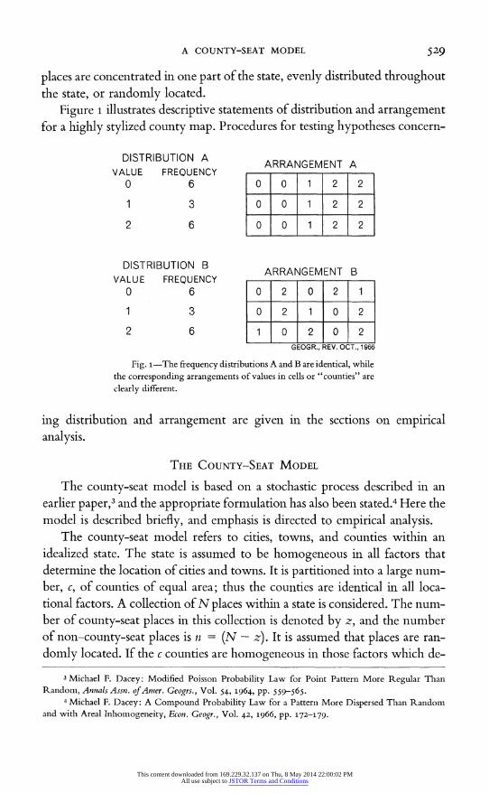
places are concentrated in one part of the state, evenly distributed throughout the state, or randomly located.

Figure 1 illustrates descriptive statements of distribution and arrangement for a highly stylized county map. Procedures for testing hypotheses concern-

DISTRIBUTION A ARRANGEMENT A VALUE FREQUENCY

0 6 0 O 1 2 2

1 3 0 O 1 2 2

2 6 0 O 1 2 2

DISTRIBUTION B ARRANGEMENT B VALUE FREQUENCY

0 6 O 2 O 2 1

1 3 0 2 1 1 2 o 6 0 2 1 2

_ _ 2 2 6 1- - - _ GEOGR., REV. OCT., 1966

Fig. 1-The frequency distributions A and B are identical, while the corresponding arrangements of values in cells or "counties" are clearly different.

ing distribution and arrangement are given in the sections on empirical analysis.

THE COUNTY-SEAT MODEL

The county-seat model is based on a stochastic process described in an earlier paper,3 and the appropriate formulation has also been stated.4 Here the model is described briefly, and emphasis is directed to empirical analysis.

The county-seat model refers to cities, towns, and counties within an idealized state. The state is assumed to be homogeneous in all factors that determine the location of cities and towns. It is partitioned into a large number, c, of counties of equal area; thus the counties are identical in all loca- tional factors. A collection of N places within a state is considered. The number of county-seat places in this collection is denoted by z, and the number of non-county-seat places is n = (N - z). It is assumed that places are randomly located. If the c counties are homogeneous in those factors which de-

3 Michael F. Dacey: Modified Poisson Probability Law for Point Pattern More Regular Than Random, Annals Assn. of Amer. Geogrs., Vol. 54, 1964, pp. 559-565.

4 Michael F. Dacey: A Compound Probability Law for a Pattern More Dispersed Than Random and with Areal Inhomogeneity, Econ. Geogr., Vol. 42, 1966, pp. 172-179.




termine the location of places, each county has an equal and independent probability of receiving a place. The distinction between county-seat places and other places requires two conditions:

A-1. Each county has an equal and independent probability of receiving a county seat, but a county contains at most one place that is a county seat.

A-2. Each county has an equal and independent probability of receiving a place that is not a county seat.

The following is also assumed:

A-3. The probabilities that a county receives county-seat places and other places are mutually independent.

THE DISTRIBUTION AND ARRANGEMENT OF PLACES

From these three assumptions, probability laws are derived that describe the distribution of the N places among the c counties and, in turn, the arrangement of counties with respect to the numbers of places they contain. Properties pertaining to distribution are derived first, then properties pertaining to arrangement.

The probability distribution of county-seat places among counties is obtained from A-1, and the probability distribution of non-county-seat places among counties is obtained from A-2. Since a place is either a county seat or not a county seat, the probability distribution of all places may be obtained from these two probability distributions.

The probability that a county receives Y county seats is obtained from A-1, and the probability is clearly

(Pr { Y = o } = 1- (1) gPr{Y=i} =c,

Pr{ Y o, = o.

The probability that a county receives W places that are not county seats is given by the binomial distribution with parameters n, the number of non- county-seat places, and 1/c, the inverse of the number of counties. By as- suming that the number of counties, c, is relatively large, the Poisson approximation to the binomial distribution may be used; thus (2) Pr { W = w} = =O, 1, 2,....

- o. elsewhere

From these two probabilities it follows, as was previously shown,' that

5 Dacey, Modified Poisson Probability Law [see footnote 3 above].



A COUNTY-SEAT MODEL 5 31

the probability that a county receives X places, where X = Y + W, is

(3) Pr IX = x= (1 -_ ) (n)xexp (-c )/x!

+ (n)XTIexp (-c-)/(x - 1)!, x = 0, 1, 2,

=0. elsewhere

Assumptions A-i and A-2 state that the probabilities of counties receiving places are random and independent events. Further, the probabilities pertaining to county-seat places and other places are mutually independent. It follows that the numbers of places in any two counties are independent events. One important spatial implication of this result is the lack of correlation between the numbers of places in adjacent counties.

The degree of correlation between numbers of places in adjacent counties is one descriptive statement on the arrangement of places. An arrangement is called random if there is no correlation between the numbers of places in pairs of counties specified by positional or distance relations. Arrangement is studied with respect to adjacent counties only, and under the assumptions of the model there is no correlation between the numbers of places in adjacent counties.

A method for describing a random arrangement of values (that is, number of places) on a county map was developed by Moran6 and others. This litera- ture and its application in a geographical context were recently reviewed by the present writer.7 The method yields the expected number and variance of pairs of adjacent counties for which one county has the value i and the other county has the value j, for i, j = o, 1, 2, ....

It is convenient to label counties in the state with the numbers 1, 2,...,

k, .. ., c. Let Lk denote the number of counties adjacent to county k. The following abbreviations are used:

( ~~~~C I A = (1/2)k i lLk,

C

(4) D = k-I 1Lk(Lk -1),

-p(x)Pr {X-x. x=i,j

The expected number of pairs of counties for which one county has i places and the other county hasj places, forj < i, is

6 p. A. P. Moran: The Interpretation of Statistical Maps, Journ. Royal Statist. Soc., Ser. B, Vol. lo, 1948, pp. 243-251.

7 Michael F. Dacey: A Review on Measures of Contiguity for Two and k-Color Maps, U. S. Governiment Research Rept.: Document Ad-612 o68, Washington, D. C., 1965.




(5a) E(i,j) = 2Ap(i)p(j),

and forj = iis (5b) E(i, i) = Ap2(i).

The variance with j x i is

(6a) V(i, j) = 2Ap(i)p(j) + Dp(i)p(j)[p(i) + p(j)] -4(A + D)p2(i)p2(j),

and for] = i the variance is (6b) V(i, i) = Ap2(i) +Dp3(i) - (A + D)p4(i).

The number of pairs of counties for which one county has i places and the other county hasj places is asymptotically distributed as a normal variate with mean E() and variance V(.). The writer has examined conditions for which the normal distribution is appropriate.8 For all analyses of arrangement undertaken in the present study, the assumption of a normal distribution does not lead to serious error in the evaluation of hypotheses.

ANALYSIS OF THE IOWA URBAN PATTERN

The empirical analysis of the central-place model used the cities and towns in Iowa as defined by the United States Bureau of the Census in 1950. To emphasize the areal application of the model, the places used for testing satisfied the census definition of place and, in addition, were areally distinct. For larger places, urbanized areas were used. Smaller places recognized by the Bureau of the Census but contiguous (as seen from a map) to a larger place were combined to form a single place for the purpose of this analysis. If any of the component places was a county seat, the combined place was called a county-seat place. Defined in this way, the 934 places listed in the 1950 census reduced to 912 areally distinct places.

The 1950, instead of the 1960, census was used because the earlier census was extracted from census publications in a form suitable for this analysis. Because only ten more places are listed in the 1960 census (944) than in 1950 (and most of these additional places are suburbs), the differences seem in- significant.

Iowa is divided into 99 counties, so that c = 99 in every case. For use of the Poisson approximation to the binomial distribution, equation (2), this value of c is sufficiently large. The number of places, N, the number of county-seat places, z, and the number of non-county-seat places, n = N -z, vary for the several hypotheses examined.

The county-seat model assumes that the counties are equal in all factors which determine the location of cities and towns. This condition is not satis-




fied by the 99 Iowa counties. The agriculture base is not completely homogeneous; there are, for example, marked differences in agricultural productivity, which are reflected in the varying rural population densities for the counties. Moreover, the counties do not even have equal areas. Although the assumptions of the model are not completely satisfied, it is hoped that the differences among counties are sufficiently small to permit an initial evaluation of hypotheses.

The validity of this county-seat model for the distribution of places was accepted," and a generalization was formulated by treating the parameters of equation (3), m = (N - z)/c and p = zlc, as random variables. This study concentrates on the underlying assumptions in terms of both the distribution and the arrangement of county-seat places, non-county-seat places, and all places.

First, the empirical validity of assumption A-2 is examined for both the distribution and the arrangement of non-county-seat places. Assumption A-1 is examined only for the arrangement of county-seat places because the content of A-1 referring to distribution is tautological. Assumption A-3 is not evaluated directly. However, the empirical evidence supports A-1 and A-2. If A-3 is true, then the observed distribution and arrangement of all places will conform to the model; hypotheses obtained from equation (3) and the con- comitant random arrangement of the resulting values are tested.

EVALUATION OF A-2

Assumption A-2 implies that the places which are not county seats are randomly distributed among counties and that, in turn, the arrangement of these places among counties is random in a spatial sense. These two aspects of randomization are tested for collections of places defined in two different ways. One collection consists of a random sample of non-county-seat places. Other collections consist of the n largest non-county-seat places for several values of n.

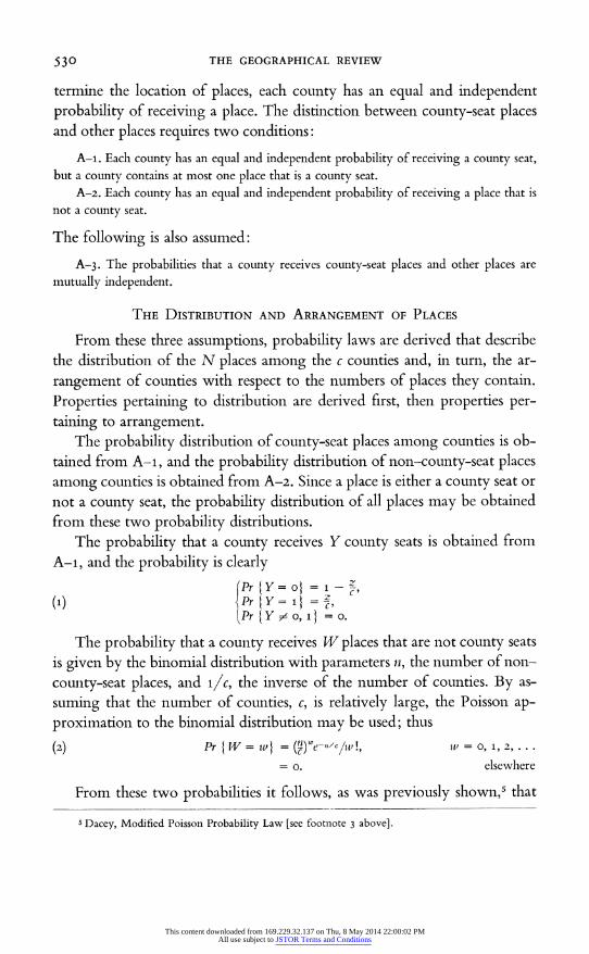
Distribution of Places among Counties. If n non-county-seat places are randomly distributed among c counties and c is relatively large, then it is well known, as stated in equation (2), that the frequency distribution of these places among counties follows the Poisson probability law with parameter equal to nlc, the average number of places per county. This property is evaluated for a random sample of places and systematic samples of larger cities and towns.

A random sample, without replacement, of 99 areally distinct places was

9 Dacey, A Compound Probability Law [see footnote 4 above].




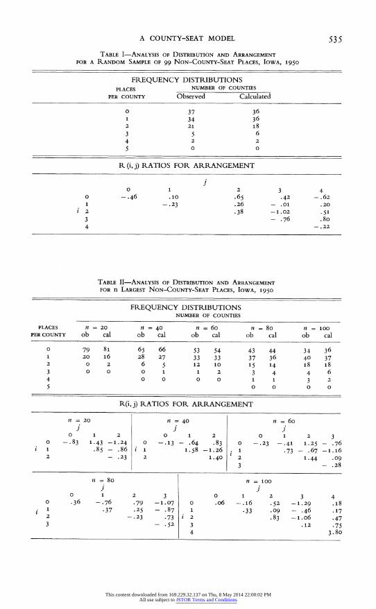
selected from the list of places that are not county seats. Table I gives the observed and calculated frequency distributions of places among counties. Ex- pected frequencies are given by equation (2) with (N - z) = n = 99 and c = 99; that is, the Poisson probability law with a parameter of unity. There is a high level of correspondence between the observed and calculated frequencies; the hypothesis of randomness is not rejected.

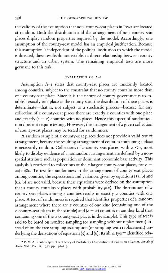
In an urban system cities and larger towns generally have greater interest than the vast number of small towns included in a random sample. For this reason, the distribution of larger places among counties is examined. The observed frequency distributions of the n largest places, for n = 20(20)100,

that are not county seats are given in Table II. The calculated frequencies are from the Poisson probability law, equation (2), with parameter n9gg. The levels of correspondence between observed and calculated values are again high, and the hypothesis of randomness is not rejected.

Arrangement of Places among Counties. Assumption A-2 implies that there is no correlation between the numbers of places in pairs of counties. For this analysis, only the correlation between pairs of adjacent counties is considered. The expected number of pairs of adjacent counties for which one county has i places and the other county has j places may be treated as a normal deviate with mean given by equation (5a, b) and variance given by equation (6a, b). The required probabilities, p(i) and p(j), are obtained from equation (2) with (N - z) = n and c = 99.

Let O(i, j) denote the observed number of adjacent counties for which one county has i places and the other county basj places. The ratio

(7) .R.(i,jI) O(i,j) - E(ij) [ V(i, j)] 1/2

may be treated as a normal variate with mean zero and unit standard devia- tion. Using the .os significance level commonly adopted by statisticians, the hypothesis of randomness is not rejected if R(i, j) lies between -2 and +2.

These ratios have been computed for the arrangements of the random sample of 99 places (Table I) and the collection of n largest non-county-seat places (Table II). The bottom part of each table gives the R(i, j) for all combinations of p(i) and p(j) for which the expected frequency, given by (2),

exceeds .015. The calculated ratios are given in matrix form; since R(i, j) = R(j, i), only values for i > j are listed. The ratios are all within the range - 2 to + 2, and the hypothesis of randomness in the arrangement of non-county- seat places among counties is not rejected.

Conclusions. The data in Tables I and II provide considerable evidence for




TABLE I-ANALYSIS oF DISTRIBUTION AND ARRANGEMENT FOR A RANDOM SAMPLE OF 99 NON-COUNTY-SEAT PLACES, IOWA, 1950

FREQUENCY DISTRIBUTIONS PLACES NUMBER OF COUNTIES

PER COUNTY Observed Calculated

0 37 36 1 34 36 2 21 18 3 5 6 4 2 2 5 0 0

R (i, j) RATIOS FOR ARRANGEMENT

,~~~~~ 0 1 2 3 4

0 -.46 .10 .65 .42 -.62 1 - .23 .26 - .01 .20

a2 .38 -1.02 .51 3 - .76 .80 4 -.22

TABLE II-ANALYSIS OF DISTRIBUTION AND ARRANGEMENT FOR n LARGEST NON-COUNTY-SEAT PLACES, IOWA, 1950

FREQUENCY DISTRIBUTIONS NUMBER OF COUNTIES

PLACES n = 20 11 = 40 n= 6o i= 8o n =oo PER COUNTY ob cal ob cal ob cal ob cal ob cal

0 79 81 65 66 53 54 43 44 34 36 1 20 16 28 27 33 33 37 36 40 37 2 0 2 6 5 12 10 15 14 18 18 3 0 0 0 1 1 2 3 4 4 6 4 0 0 0 0 1 1 3 2 S 0 0 0 0

R(i, j) RATIOS FOR ARRANGEMENT

n =20 n = 40 n= 6o

0 1 2 0 1 2 0 1 2 3 0 -.83 1.43 -1.24 0 -.13 - .64 .83 0 -.23 -.41 1.25 - .76

i 1 .85 - .86 i 1 1.58 -1.26 1 .73 - .67 -1.16 2 - .23 2 1.40 2 1.44 .09

3 - .28

il = 80 11 =1 00

0 1 2 3 0 1 2 3 4 0 .36 -.76 .79 -1.07 0 .o6 -.16 .52 -1.29 .18 1 .37 .25 - .87 1 .33 .09 - .46 .17 2 -.23 .73 i 2 .83 -i.o6 .47 3 - .52 3 .12 .75

4 3.80




the validity of the assumption that non-county-seat places in Iowa are located at random. Both the distribution and the arrangement of non-county-seat places display random properties required by the model. Accordingly, one assumption of the county-seat model has an empirical justification. Because this assumption is independent of the political institution to which the model is directed, these results do not establish a direct relationship between county structure and an urban system. The remaining empirical tests are more germane to this task.

EVALUATION OF A-1

Assumption A-1 states that county-seat places are randomly located among counties, subject to the constraint that no county contains more than one county-seat place. Since it is the nature of county governments to establish exactly one place as the county seat, the distribution of these places is determinate-that is, not subject to a stochastic process-because for any collection of z county-seat places there are exactly z counties with one place and exactly (c - z) counties with no places. Hence this aspect of randomization does not require testing. However, the arrangement of a given collection of county-seat places may be tested for randomness.

A random sample of z county-seat places does not provide a valid test of arrangement, because the resulting arrangement of counties containing a place is necessarily random. Collections of z county-seat places, with z < c, most likely to display evidence of a nonrandom arrangement are defined by a nonspatial attribute such as population or dominant economic base activity. This analysis is restricted to collections of the z largest county-seat places, for z = 20(20)8o. To test for randomness in the arrangement of county-seat places among counties, the expectations and variances given by equations (5a, b) and (6a, b) are not valid, because these equations were derived on the assumption that a county contains x places with probability p(x). The distribution of z county-seat places among c counties results in exactly z counties with one place. A test of randomness is required that identifies properties of a random arrangement where there are z counties of one kind (containing one of the z county-seat places in the sample) and (c - z) counties of another kind (not containing one of the z county-seat places in the sample). This type of test is said to be based on nonfree sampling (or sampling without replacement) instead of on the free sampling assumption (or sampling with replacement) underlying the derivations of equations (5) and (6). Krishna IyerI0 identified rela-

'o P. V. A. Krishna Iyer: The Theory of Probability Distributions of Points on a Lattice, Aninals of

Math. Stat., Vol. 21, 1950, pp. 198-217.




tions between the free sampling and nonfree sampling cases. The results were summarized by the present writer,", and the equations required for this analysis are written below. The expectation and variance for the arrangement of two values, o and 1, under the assumption of nonfree sampling are denoted by E'(-) and V'(). The symbol r(x) denotes the falling factorial

(8) r(x) = r(r -1) ... (r -x + 1).

The three sets of equations required for the analysis of arrangement of z county-seat places among c counties with z < c are

E(1, 1i) = Az(2) /C(2),

(9a) V'(1, 1) = Az(2)/c(2) +Dz(3)(3)3) +(A2 - A - D)z(4)/c(4) - (Az(2)/C(2))2;

Et(o, o) = A(c -Z)(2)IC(2)

(9b) V"(o, o) = A(c -Z) (2) /C(2) + D(c -Z) (3) /c(3)

+(A- - A - D)(c -Z)(4)/C(4) - (A(c -z)(2)/c(2))2;

E'(o, 1) = 2Az(c -Z)AW)

(9C) V(o, 1) = 2Az(c -Z)/C(2) + Dz(c - z)(c -2)/C(3)

+14(A2 - A - D)z(2)(c - Z)(2) C (4)- 4(Az(c -z)/C(2))2.

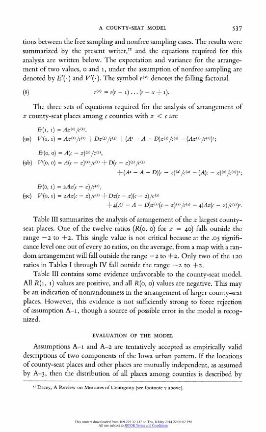
Table III summarizes the analysis of arrangement of the z largest county- seat places. One of the twelve ratios (R(o, o) for z = 40) falls outside the range-2 to +2. This single value is not critical because at the .os significance level one out of every 20 ratios, on the average, from a map with a random arrangement will fall outside the range-2 to +2. Only two of the 120

ratios in Tables I through IV fall outside the range-2 to +2.

Table III contains some evidence unfavorable to the county-seat model. All R(1, 1) values are positive, and all R(o, o) values are negative. This may be an indication of nonrandomness in the arrangement of larger county-seat places. However, this evidence is not sufficiently strong to force rejection of assumption A-1, though a source of possible error in the model is recognized.

EVALUATION OF THE MODEL

Assumptions A-1 and A-2 are tentatively accepted as empirically valid descriptions of two components of the Iowa urban pattern. If the locations of county-seat places and other places are mutually independent, as assumed by A-3, then the distribution of all places among counties is described by

II Dacey, A Review on Measures of Contiguity [see footnote 7 above].




TABLE III-ANALYSIS OF ARRANGEMENT FOR Z LARGEST COUNTY-SEAT PLACES

R(i,j) RATIOS FOR ARRANGEMENT

Z =20 Z 40 Z_ 6o z = 80

0 1 0 1 0 1 0 1 0 -1.15 .31 .0 -2.33 1.26 .o -1.19 - .58 i0 -.76 - .48

t 1 1.32 1 55 1 1.85 1 1.03

TABLE IV-ANALYSIS OF DISTRIBUTION AND ARRANGEMENT FOR N LARGEST PLACES, IOWA, 1950

FREQUENCY DISTRIBUTIONS Parameters

N=20 N=40 N=6o N= 8o N= loo N= 2oo z = 18 z = 34 z = 50 z = 66 z = 78 z =98

PLACES NNUMBER OF COUNTIES PER

COUNTY ob cal ob cal ob cal ob cal ob cal ob cal

0 80 80 6o 61 43 44 28 29 15 17 0 0 1 18 19 38 36 52 50 62 61 69 66 34 35 2 1 0 1 2 4 5 9 8 14 14 38 36 3 0 0 1 1 2 21 19 4 3 6 5 3 2 6 0 1

R(i, j) RATIOS FOR ARRANGEMENT

N =20 N = 40 J J

0 1 0 1 2 0 -.12 -.21 0 -1.04 1.50 -.86 1 .99 i .82 -.84

2 -.29

N = 60 N- 80

0 1 2 0 1 2 0 -.87 - .08 -.74 0 -.38 -.92 - .40 i 1 1.25 .04 i 1 .54 1.21 2 -.62 2 - 37

N = loo N 200

0 1 2 3 1 2 3 4 5 0 -.39 -.80 -.66 -.14 1 .08 -.22 .29 -1.32 .15 1 .72 .21 .18 2 .26 1.23 -1-35 .12 2 .80 -.81 i 3 1.26 -1.43 .40

3 -.22 4 .o6 .67 5 3.58




equation (3), and the observed frequencies are arranged in a random manner among the Iowa counties.

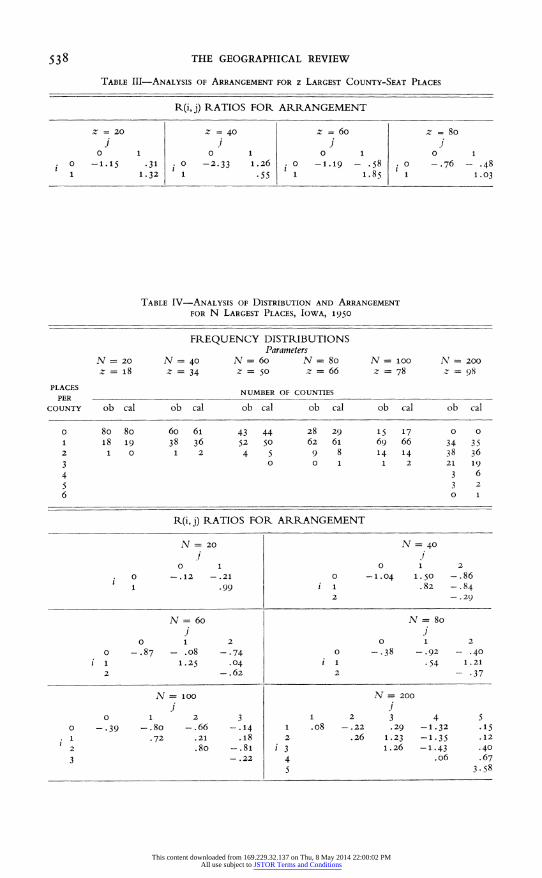
Distribution of All Places among Counties. Equation (2) describes the distribution of non-county-seat places among counties, and, by definition, equation (1) describes the distribution of county-seat places among counties. If the distributions of the two kinds of places are independent, equation (3) describes the distribution of all places among counties. This hypothesis is examined only for collections of cities and larger towns. Random samples of places contain relatively few (approximately 10 percent) county seats and hence do not provide a very severe test of distribution. Table IV gives the frequency distributions of the N largest places among the Iowa counties for N = 20(20)100, 200.

The model asserts that the frequency distribution of places among counties depends on the number of counties, c, and the number of county-seat places, z, in a collection of N places; c = 99 always, and N and z are listed in Table IV. Calculated frequencies were obtained from equation (3) and are listed in Table IV. It is noted that the calculated frequencies are obtained in- dependently of the observed frequency distributions. A closer correspondence between observed and calculated values would undoubtedly be obtained if the parameters of equation (3) were estimated (by method of moments or method of maximum likelihood) from the observed frequency distributions. Because the parameters have a substantive interpretation, it was not necessary to estimate parameters from the data, and a relatively rigorous test of the hypothesis obtained from equation (3) is possible.

Agreement between observed and calculated values is reasonably good. There is, however, a bias toward overestimation (usually by one) of the number of counties with no places, and a bias toward underestimation of the number of counties with exactly one place. Because of this systematic bias, the model is not completely satisfactory. However, the magnitude of the bias is small, and the writer is not willing to reject the model at this stage of analysis. A sterner judge might decide otherwise.

A Limiting Property. The value of z is never greater than c, and the frequency distribution (3) has a limiting property as z approaches or, possibly, is equal to c. The probability law defined by equation (3) has two terms. The first term is multiplied by (1 - zlc), so that as z approaches c this term goes to o and the entire mass of the probability law shifts to the second term. The second term is a Poisson probability shifted up by one value. For z = c, each county necessarily contains at least one place (a county seat) and, by A-2, the remaining n = (N - c) places are randomly distributed among counties.




This limiting property is seen in Table IV. For N = 200, z/c = 98/99, and the expected number of counties containing no places, from equation (3), is less than o.oo5c.

Arrangement of All Places among Counties. The random arrangement of non-county-seat places implied by A-2 was supported by empirical evidence. The random arrangement of county-seat places implied by A-1 was less clearly established. Thus the outcome of this test for randomness in the arrangement of all places is critical to the evaluation of the county-seat model. The hypothesis of randomness is tested by the ratios R(i, j) with the expected values and variances given by equations (5a, b) and (6a, b) respectively. The probabilities p(i) and p(j), as defined in equation (4), are obtained from equation (3). The observed ratios for the N largest places are given in the lower half of Table IV in matrix form. Ratios are given for all combinations of values for which the expected number of counties with x places exceeds 1.5. Only one ratio is outside the range -2 to +2, and the hypothesis of random arrangement is not rejected. However, it is noted that ratio values with i = o are largely negative. This bias probably reflects that the calculated frequency distributions overestimate the number of counties with no places rather than nonrandomness in the arrangement of counties.

EVALUATION AND INTERPRETATION OF RESULTS

A simple model for the distribution and arrangement of places in an urban system was described. It was extensively tested in terms of cities and larger towns in the state of Iowa. Any model as simple as this county-seat model is doomed to fail some experimental test. However, by selecting a study region for which conditions of the model were approximately satisfied, reasonably satisfactory agreement between observed and calculated values was found. It was properly noted that empirical evidence disclosed some inadequacies in the model, but it was not felt that the discrepancies were sufficiently large to justify its immediate rejection.

Evaluation of a model depends on factors other than goodness of fit. These include its generality, its consistency with more general theories, and its status vis-a-vis alternative models for the same phenomenon.

This county-seat model was evaluated only for one urban pattern-an inadequate basis for asserting generality. Although this is the most extensive

test of the model the writer has undertaken, aspects of the model (pertaining to distribution) were considered in the more general context of treating the parameters of equation (3) as random variables.I2 This allowed application

12 Dacey, A Compound Probability Law [see footnote 4 above].




of the model to large regions for which the assumption of homogeneous counties is unacceptable. The model for inhomogeneous situations was tested for the distributions of places among counties in a six-state Midwestern area and for the entire United States. Levels of correspondence between observed and calculated values were acceptable.

The probability law (3) was initially derived in a different context,'3 and it was shown that the same stochastic process was applicable to the distribution of farms on the Tonami Plain in Japan. Completed, but unpublished, research indicates that the basic model has a number of applications. The present analysis does not constitute an isolated application. Accordingly, generality is claimed for the model.

This county-seat model conflicts with the classical formulation of central- place theory. However, it has been shownI4 that central-place theory is essen- tially a statement of space filling, and the county-seat model is compatible with the concept of space filling. A report in preparation interprets central- place theory in terms of this county-seat model. At this stage of the investiga- tion it is safe only to assert that the county-seat model does not conflict with the basic notions of central-place theory, though it may be incompatible with the particular formulations given by Christaller and L6sch.

The county-seat model is consistent with very simple observations on the structure of county governments. Even the casual observer of the American urban landscape recognizes that there is a high probability that a large place is a county seat, and, in turn, the probability is high that the county seat is the largest place in the county. Because county seats were selected by fiat or popular election at an early stage in the development of an urban system, it

seems incontrovertible that the political institution of county governments and the pragmatics of selecting county seats have had a strong effect on the pattern of cities and larger towns. A detailed report on the selection of county seats in Iowa has been compiled by Swisher,'5 which contains many fasci- nating tales of intrigue and comedy.

The county-seat model simply makes explicit the dependence of the urban system on this political process without attempting to incorporate the com- plicated nuances of political reality. Instead, the institution of county seats is interpreted in the areal context of urban systems by abstracting the outcome of political processes to a geographical statement summarizing the distribu-

'3 Dacey, Modified Poisson Probability Law [see footnote 3 above]. '4 Michael F. Dacey: The Geometry of Central Place Theory, Geografiska Annaler, Vol. 47 B, 1965,

pp. 111-124.

I'J. A. Swisher: The Location of County Seats in Iowa, Iowa Journ. of History and Politics, Vol. 22,. 1924, pp. 89-128, 217-294, and 323-362.




tion and arrangement of places. Since randomness defines a simple type of distribution and arrangement, the county-seat model is a somewhat naive formulation of a basic institutional factor. A critic would be justified in asserting that the interpretation of the county structure lacks geographical sophistication.

Central-place theory provides an alternative description for the areal pattern of an urban system. The pattern of central-place theory is a completely determined hexagonal point lattice, and it is inconceivable that any observed urban pattern would conform to the lattice arrangement. Although central- place theory is helpful for an understanding of urban systems, its lack of empirical validity is obvious, and its predictive ability is nil because point estimates (geometrically determined lattice locations) have infinite variance. Because the county-seat model and central-place theory approach urban patterns with entirely different objectives, it is not meaningful to demand empirical analysis of central-place patterns. Evidently the county-seat model is the only statement on the distribution and arrangement of an urban system that satisfies the prerequisites for empirical analysis and has, with some success, described observed patterns.



a county-seat model for the areal pattern of an urban system

Documents