a consistent two-factor model for pricing temperature
TRANSCRIPT
A consistent two-factor model for pricing temperature
derivatives
Andreas Groll ∗ Brenda Lopez-Cabrera † Thilo Meyer-Brandis ‡
Abstract
We analyze a consistent two-factor model for pricing temperature derivatives that
incorporates the forward looking information available in the market by specifying a model
for the dynamics of the complete meteorological forecast curve. The two-factor model is
a generalization of the Nelson-Siegel curve model by allowing factors with mean-reversion
to a stochastic mean for structural changes and seasonality for periodic patterns. Based
on the outcomes of a statistical analysis of forecast data we conclude that the two-factor
model captures well the stylized features of temperature forecast curves. In particular,
a functional principal component analysis reveals that the model reflects reasonably well
the dynamical structure of forecast curves by decomposing their shapes into a tilting and
a bending factor. We continue by developing an estimation procedure for the model,
before we derive explicit prices for temperature derivatives and calibrate the market price
of risk (MPR) from temperature futures derivatives (CAT, HDD, CDD) traded at the
Chicago Mercantile Exchange (CME). The factor model shows that the behavior of the
implied MPR for futures traded in and out of the measurement period is more stable
than other estimates obtained in the literature. This confirms that at least parts of
the irregularity of the MPR is not due to irregular risk perception but rather due to
∗Mathematical Institute, University of Munich, Theresienstrasse 39, 80333 Munich, Germany. Email:
<[email protected]>†Institute for Statistics, Humboldt-Universitat zu Berlin, Spandauer Straße 1, 10178 Berlin, Germany.
Email:< [email protected]>‡Mathematical Institute, University of Munich, Theresienstrasse 39, 80333 Munich, Germany. Email:
1

information misspecification. Similar to temperature derivatives, this approach can be
used for pricing other non-tradable assets.
Key words: factor models, consistency, pricing and hedging, weather derivatives, market
price of risk
1 Introduction
In the last years weather derivatives (WD) have emerged to hedge weather variability. This
leads to the question how such derivatives are priced and hedged. In contrast to other assets,
the pricing of weather derivatives has some challenges since the underlying, contingent on
temperature or rain, is not tradeable and the classical Black, Merton and Scholes framework fails
since hedging principles cannot be applied. Different streams for pricing weather derivatives are
found in the literature: econometric modeling of the underlying dynamics ([12], [10]) followed
by risk neutral pricing, equilibrium models [13], indifference pricing models [11], index modeling
and burn analysis [23].
In the context of no-arbitrage pricing, there has been some work to calibrate and study
the complex structure of the risk premium in temperature derivative prices, or the market
price of risk (MPR). The contributions of [13] and [27] study the MPR of weather deriva-
tives as an implicit parameter in a generalization of the Lucas’ (1978) equilibrium framework.
Equivalent changes of measure with a parametrized time-dependent MPR to get no arbitrage
futures/options prices written on different temperature indices were introduced in [10], how-
ever the calibration of the MPR was not performed. [22] estimate the MPR from the Taiwan
Stock Exchange Capitalization Weighted Stock Index and use it as a proxy for the MPR on
temperature option prices.
While most of the papers on temperature derivative pricing impose by assumption a zero
or constant MPR ([14], [13], [22], [27] and [1]), a more differentiated analysis conducted in
[19], [8], [7], [9] and [20] actually reveals a complex time varying and stochastic behavior of
the MPR. However, we believe that at least parts of the irregular behavior of the MPR is
not due to irregular risk pricing of the market but due to a misspecification of most models
that are used to calibrate market prices: forward looking information about the temperature
2

available to the market is not taken into account in the information modeling. The usual
assumption that all information available to the market is incorporated in the underlying,
i.e. the information filtration is generated by the underlying, might be acceptable for storable
assets (classical financial markets). However, for non-storable underlyings (like temperature
or electricity) this assumption is fundamentally wrong: lots of meteorological forward looking
information available to the market is not reflected in the past evolution of temperature. Hence,
an appropriate model for the pricing of temperature derivatives should take into account the
information about meteorological forecasts available to the market participants.
There is only few literature dealing with the incorporation of meteorological forecast into
weather derivative pricing. [1] suggests, without a model, to incorporate forecasts for short-
term pricing. How to use single and ensemble forecasts to derive probabilistic weather forecasts
for weather derivative pricing is described in [23]. [31] incorporates the seasonal forecast in the
temperature process, by assuming the unconditional mean temperature as a linear combinations
of above-normal (warm), near-normal, and below-normal (cool) mean temperature processes.
[6] apply the theory of enlargement of filtration to describe all information available in the
market and with it estimate information premiums for given filtrations strictly bigger than the
one generated by the underlying. The model from [6] is applied in [28]. There, assuming a
MPR equal to zero, it is shown that incorporating weather forecast gives better accurates of
market prices. [18] also used an enlargement of the filtration set with weather forecasts by
modeling the temperature dynamics process with a larger time series that consists of historical
and weather forecast data. Another empirical study of the information premium is described
in [5]. The challenge of working with the theory of enlargement of filtrations is the analytic
tractability of the forward looking information. In [14] an index modeling approach is used and
it is also shown that weather forecasts significantly influence prices. [21] models temperature
forecasts by a finite dimensional factor model and guarantees consistency with the martingale
dynamics of temperature forecasts. However, no empirical analysis is shown there.
The idea in [21] is two include forward looking information available in the market into
temperature modeling by specifying a model for the complete meteorological temperature fore-
cast curve. More precisely, given a filtered probability space (Ω,F ,Ft≥0,P) fulfilling the usual
3
conditions, it is assumed that the meteorological forecast f(t;T ) at time t of the temperature
τ(T ) at time T is an unbiased estimator of the temperature in the sense that
f(t;T ) = E[τ(T )|Ft] . (1)
For fixed forecast time T , the forecast process f(·;T ) is thus a martingale under the real world
probability measure P with respect to the flow of available information Ft. Next, the evolution
of the forecast curves is modeled by a factor model
f(t, T ) = H(T − t, Z(t)),
where
• H(x, z) : R+ × Rm → R is a given curve family;
• x = T − t is time to forecast time;
• Z(t) is an Rm-valued factor process given by an Ito diffusion
dZ(t) = b(Z(t)) dt+ σ(Z(t)) dW (t), Z(0) = z0,
with W (t) a d-dimensional Ft-Brownian motion.
By setting T = t, we then obtain the dynamic model for the temperature τ(t) = f(t; t) which
now is driven by information contained in the complete forecast curve.
A factor model is called consistent if H(T − t, Z(t)) is an Ft-martingale for any fixed T ≥ 0
in accordance with (1). Given a curve family H(x, z), the consistency requirement imposes
certain restrictions on admissible drift coefficients b(z) and volatility coefficients σ(z) which,
for certain types of families H(x, z), are characterized in [21].
The purpose of this paper is to perform an empirical analysis of temperature and tempera-
ture forecast data in the context of a specific two-factor model introduced in [21]. To this end
we adhere to the following modus operandi.
4

First, a descriptive statistical analysis of the temperature and temperature forecast data is
performed. In particular, a functional principal component analysis (FPCA) is applied which
provides a natural choice for the number of factors and characterizes curve co-movements in
terms of common factors.
Then we introduce the two-factor model and analyze its properties. Based on the previously
performed empirical analysis of curve data we conclude that the consistent two-factor model
for pricing temperature derivatives explains the stylized facts of historical and forecast temper-
ature curves (seasonality, seasonal variance, exponential decaying autocorrelation) accurately
by decomposing the data curve shapes into two factors describing the mean-reversion in the
long horizon and tilting or bending of the curves in the short horizon. The two-factor model
is within the framework of the Nelson-Siegel curve model, incorporating time-dependent fac-
tors for structural changes (namely the impact of additional forward looking information) and
seasonality for periodic patterns. It extends other models proposed in the weather derivative
literature by including a mean-reversion to a stochastic mean level.
Next, we specify and implement an iterative two-step algorithm for the estimation of our
model. The algorithm switches between a joint maximization of the likelihood with respect to
the unknown model parameters and a least-squares estimation step of the second factor of the
two-factor model.
Finally, the results from [21] are extended, as we derive explicit prices for temperature
derivatives written on Cumulative Average Temperature (CAT), Heating Degree Days (HDD)
and Cooling Degree Days (CDD) and quantify risk expectations of market participants by ana-
lyzing the dynamics of the market price of risk (MPR) of the associated equivalent martingale
measure (EMM). With the information available in the market data (historical temperature,
meteorological forecast and futures prices), we calibrate the MPR of temperature derivatives
(CAT, CDD, HDD) traded at the Chicago Mercantile Exchange (CME). The factor model
shows that the behavior of the implied MPR for futures traded in and out of the measurement
period is more stable than other estimates such as e.g. obtained in [19]. This confirms that
irregularity of the MPR is not due to irregular risk perception but rather due to information
misspecification. Similar to temperature derivatives, we conclude that this approach can be
5

used for pricing other non-tradable assets.
Our article is structured as follows. In Section 2 we present the empirical analysis for the
forecast data. Section 3 introduces the consistent two factor model and presents an estimation
algorithm. The pricing of temperature derivatives with the proposed factor model is developed
in Section 4, together with the calibration of the MPR. Section 5 concludes the paper. All com-
putations in this paper were carried out in the statistical program R ([25]). The temperature
and weather derivative data was obtained from Bloomberg and is available in the Risk Data
Center (RDC) of the CRC 649 Economic Risk (http://sfb649.wiwi.huberlin.de/).The meteoro-
logical forecast data was obtained from WeatherOnline. To simplify notation, in the following
dates are denoted with yyyymmdd format.
Throughout the article we will use the following notations for different forecast curves,
depending on the context. As already introduced in (1), f(t; t + x) denotes the forecast curve
implied by our factor model at time t of the temperature τ(t+x) at time t+x. The notation ft;t+x
stands for a time series of observed (discrete) forecast data at time points t of the temperature
at time t+ x, while ft(x) is a smooth (continuous) interpolation of the observed forecast time
series at time t.
2 Empirical analysis of temperature forecast curves
In this section we present an empirical analysis of the temperature and point temperature
forecast data of the cities New York and Berlin1 for the time period 20081229 - 20131003 and
20081229 - 20101202, respectively. The observed forecast at time t of the average temperature at
time t+x is denoted by ft;t+x, x = 0, . . . , 14, i.e. each forecast curve consists of the contemporary
temperature (x = 0) together with the average forecast (which we obtained from the minimum
and maximum) of the next 14 days’ temperatures. Adjusting the data for measurement errors
and missing values2, we end up with 1740 entire forecast curves for New York and 411 entire
1Data source: New York Laguardia Airport and Tempelhof Airport Meteorological forecast data from Weath-erOnline. We thank Dr. Ulrich Romer and Herrad Werner for providing us the data. Note here that as ourforecast and temperature data had to be obtained from different providers, this bears a risk of inconsistenciesin the data.
2For New York on 11 days and for Berlin on 6 days the entire forecast curve was missing; here we imputed,if possible, the forecast of a weather station nearby or by averaging over the preceding and subsequent day.For some other days the forecasts of the last or the last two days of the forecast period were missing; here we
6

forecast curves for Berlin. Figure 1 illustrates the structure of the temperature data together
with the forecast curves of three selected days.
0 2 4 6 8 10 12 14
−10
010
2030
forecast period
tem
pera
ture
(in
C°)
0 2 4 6 8 10 12 14
−5
05
1015
2025
forecast period
tem
pera
ture
(in
C°)
Figure 1: Temperature data (x = 0) together with the forecast curves (x = 1, . . . , 14) of threeselected days (t = 20090111, 20090526, 20090804)) for New York (top) and Berlin (bottom).
2.1 Unbiasedness
As already stated in the introduction, a central issue in this article is to incorporate forward
looking information available in the market by specifying a model for the complete forecast
curve. In our approach we assume that the forecast is unbiased in the sense that it represents
the expected temperature given all available information (see Equation (1)). We first analyze if
this assumption is confirmed in our time series by comparing expected forecasts with expected
temperatures. We use the average differences of true temperatures and forecasts for the different
imputed by the forecast of the preceding day.
7

forecast horizons x, i.e.
Dx :=1
Nx
Nx∑i=1
fti;ti+x − fti+x;ti+x, x = 1, . . . , 14
where Nx denotes the number of available pairs of true temperatures and corresponding fore-
casts for these temperatures. While for Berlin the differences seem to vary randomly around
zero, for New York the forecasts seem to slightly overestimate the true temperature, which in
fact indicates that there are some inconsistencies in the New York data as already suspected in
Footnote 1. Additionally, in order to assess the general predictive quality of the forecasts, we
also present the average of the absolute differences for different forecast horizons, i.e.
|Dx| :=1
Nx
Nx∑i=1
|fti;ti+x − fti+x;ti+x|, x = 1, . . . , 14.
As expected, |Dx| is generally increasing for larger forecast horizons, compare Table 1, but is
still in a moderate range for both cities. Though for Berlin the forecasts seem less biased, in
summary we can say that for both cities the forecasts serve as proper predictions of the true
temperatures.
x 1 2 3 4 5 6 7 8 9 10 11 12 13 14
DxNew York .08 .21 .29 .33 .35 .44 .51 .75 .99 1.14 1.25 1.34 1.42 1.45Berlin -.04 -.06 .05 -.02 .06 .17 .15 -.04 -.07 .07 .22 .35 .51 .60
|Dx|New York .95 1.15 1.31 1.52 1.70 1.95 2.16 2.36 2.63 2.79 2.90 3.05 3.13 3.20Berlin 1.55 1.60 1.68 1.61 1.83 1.86 2.12 2.25 2.21 2.42 2.63 2.73 2.96 3.09
Table 1: Average of standard and absolute differences of true temperatures and forecasts forthe different forecast horizons x and different locations.
2.2 De-seasonalization
Based on the true average temperatures3 of New York - Laguardia airport for the time period
1997-2012 and of Berlin - Tempelhof airport for the time period 1948-2011, a linear trend
(for possible temperature increases due to global warming) together with a periodic seasonal
trend component have been estimated using non-linear least squares estimation (NLSE), which
is implemented e.g. in the R-function nls (see [3]) and is based on the following truncated
3Minimum, maximum and average temperatures are provided by CME website.
8

Fourier series
Λ(t) = a1 + a2t+ a3 cos
(2π(t− a4)
365
)(2)
for parameters ak, k = 1, . . . , 4 and with time t (daily scale). Note that one could refine this
seasonality function by adding more and more periodic terms, but this will increase the number
of parameters. Alternatively, non-parametric techniques could be used as described e.g. in [18].
Next, the temperature time series and the 14 forecast time series for the different forecast
periods of New York and Berlin are de-seasonalized by subtracting the trend function Λ(t)
from Equation (2). Exemplarily, the de-seasonalized time series for the true temperature and
a forecast period of 6 days are illustrated in Figure 2 for both locations. For the set of forecast
curves from Figure 1, the corresponding de-seasonalized forecast curves are shown in Figure 3.
0 500 1000 1500
−10
010
2030
temperature
day
tem
pera
ture
(in
C°)
0 500 1000 1500
−10
010
2030
6−days forecast
day
tem
pera
ture
(in
C°)
0 100 200 300 400
−10
010
20
temperature
day
tem
pera
ture
(in
C°)
0 100 200 300 400
−10
010
20
6−days forecast
day
tem
pera
ture
(in
C°)
Figure 2: Origninal (gray) and de-seasonalized time series (black) for New York (top) andBerlin (bottom), exemplarily for the true temperature and the “6 days” forecast period.
9

0 2 4 6 8 10 12 14
−15
−10
−5
05
forecast period
(des
easo
naliz
ed)
fore
cast
cur
ves
0 2 4 6 8 10 12 14
−15
−10
−5
05
forecast period
(des
easo
naliz
ed)
fore
cast
cur
ves
Figure 3: Three de-seasonalized forecast curves for New York (top) and Berlin (bottom).
2.3 Distributional properties of the forecast data
Next, we graphically analyze the assumption of normality for the de-seasonalized time series.
For both New York and Berlin we found no distinct violations in the corresponding q-q-plots
(see Figure 4). In the next step, we apply a conventional statistical test on normality, the
Kolmogorov-Smirnov test. It rejects the assumption of normality never for both cities at a
significance level of α = 0.01. Hence, the assumption of normality seems justifiable, which is in
accordance with the theoretical properties of the two-factor model presented in Section 3.1.
2.4 Stationarity and autocorrelation
In the next step we check for intertemporal autocorrelation and stationarity of the temperature
and forecast time series. The partial autocorrelation plots indicate that there is significant
10

−4 −2 0 2 4
−4
−2
02
4
q−q−plot temperature
Theoretical Quantiles
Sam
ple
Qua
ntile
s
−4 −2 0 2 4
−4
−2
02
4
q−q−plot forecast 6 days
Theoretical Quantiles
Sam
ple
Qua
ntile
s
−4 −2 0 2 4
−4
−2
02
4
q−q−plot temperature
Theoretical Quantiles
Sam
ple
Qua
ntile
s
−4 −2 0 2 4
−4
−2
02
4
q−q−plot forecast 6 days
Theoretical Quantiles
Sam
ple
Qua
ntile
s
Figure 4: Selected q-q-plots of the de-seasonalized time series (temperature and six day forecast)for New York (top) and Berlin (bottom).
autocorrelation up to about three lags (except for some single artifacts), which is in accordance
with the literature e.g. in [10] and [19]. Figure 5 exemplarily shows the partial autocorrelations
for the temperature and a forecast period of six days for both locations. Moreover, for New York
the corresponding augmented Dickey-Fuller test, implemented in the R-function adf.test,
confirms that all 15 time series (true temperature and 14 forecasts) are stationary and the null
hypotheses corresponding to the presence of a unit root can be rejected for all tests at a level
of significance of α = 0.01. For Berlin we get similar results and the presence of a unit root is
rejected at α = 0.01 for the true temperature as well as for the forecast horizons x ∈ 1, . . . , 9.
For the forecast horizons x ∈ 10, . . . , 14 the presence of a unit root is only rejected at a level
of significance of α = 0.05.
11

5 10 15 20
−0.
20.
20.
6
Lag
Par
tial A
CF
Temperature
5 10 15 20
0.0
0.2
0.4
0.6
Lag
Par
tial A
CF
Forecast 6 days
5 10 15 20
0.0
0.4
0.8
Lag
Par
tial A
CF
Temperature
5 10 15 20
0.0
0.4
0.8
LagP
artia
l AC
F
Forecast 6 days
Figure 5: Partial autocorrelations of the temperature and the forecast time series, exemplarilyfor a forecast period of six days, for New York (top) and Berlin (bottom).
2.5 Functional principal component analysis
In this section, we further explore the features characterizing typical (de-seasonalized) forecast
curves, in particular we analyze by how many factors the curves are driven. A classical approach
in this direction is principal component analysis (PCA), providing an informative way of looking
at the covariance structure.
However, in the two-factor model presented in Section 3.1 the forecast curve at a certain
time t is considered as a smooth continuous function of the forecast horizon x. This suggests to
regard our data in a functional context. Furthermore, several authors such as [29] and [30] state
that the computation of PCA runs into serious difficulties in analyzing functional data because
of the so-called “curse of dimensionality” (see also [4]). Following [29], these difficulties can be
overcome by functional principal components analysis (FPCA, i.e. PCA extended to functional
data; see [26, Chapter 8.]), which provides a more informative way of examining the sample
covariance structure than conventional PCA and which also complements a direct examination
of the variance-covariance structure and characterizes curve comovements in terms of common
factors. Besides, if necessary, FPCA allows to incorporate regularization.
Consequently, we transform all 1740 forecast curves of New York and all 411 forecast curves
12
of Berlin into smooth functional data objects using a penalized basis function approach de-
scribed in [26], which is implemented in the R-package fda. Note here that also the functional
mean of a set of N different functions can be derived following [26], who provide a mean()
method for functional data objects using
g(t) = N−1N∑i=1
gi(t)
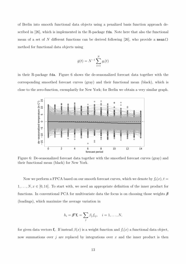
in their R-package fda. Figure 6 shows the de-seasonalized forecast data together with the
corresponding smoothed forecast curves (gray) and their functional mean (black), which is
close to the zero-function, exemplarily for New York; for Berlin we obtain a very similar graph.
0 2 4 6 8 10 12 14
−15
−10
−5
05
1015
forecast period
de−
seas
onal
ized
tem
pera
ture
(in
C°)
Figure 6: De-seasonalized forecast data together with the smoothed forecast curves (gray) andtheir functional mean (black) for New York.
Now we perform a FPCA based on our smooth forecast curves, which we denote by ft(x), t =
1, . . . , N, x ∈ [0, 14]. To start with, we need an appropriate definition of the inner product for
functions. In conventional PCA for multivariate data the focus is on choosing those weights βββ
(loadings), which maximize the average variation in
hi = βββᵀfi =∑j
βjfij, i = 1, . . . , N,
for given data vectors fi. If instead β(x) is a weight function and fi(x) a functional data object,
now summations over j are replaced by integrations over x and the inner product is then
13
defined by∫β(x)fi(x)dx, where the integral is defined over the range of x (as we consider 14
days forecasts together with the contemporary temperature, we have x ∈ [0, 14]). Consequently,
within functional PCA, for a given weight function β(x) the corresponding principal component
score is given by
hi =
∫β(x)fi(x)dx.
In the first FPCA step, a weight function β1(x) is chosen to maximize the sum
1
N
∑i
h2i1 =1
N
∑i
(∫β1(x)fi(x)dx
)2
,
subject to the constraint ||β1||2 :=∫β1(x)2dx = 1, which is the continuous analog of the unit
sum of squares constraint used in the conventional multivariate PCA. Similar to multivariate
PCA, this procedure is carried out in subsequent steps for further weight functions βm(x),m =
2, . . . , p, each satisfying the orthogonality constraint∫βk(x)βm(x)dx = 0, k < m, up to a
maximum of p weight functions, which in our case corresponds to the number of basis functions
determined in the penalized basis function approach. Hence, each weight function defines the
most important mode of variation in the curves subject to each mode being orthogonal to all
modes defined on previous steps. For the computational details concerning the FPCA we refer
to [26, Chapter 8.4].
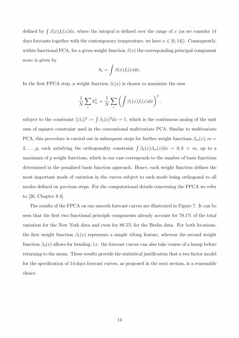
The results of the FPCA on our smooth forecast curves are illustrated in Figure 7. It can be
seen that the first two functional principle components already account for 78.1% of the total
variation for the New York data and even for 88.5% for the Berlin data. For both locations,
the first weight function β1(x) represents a simple tilting feature, whereas the second weight
function β2(x) allows for bending, i.e. the forecast curves can also take course of a hump before
returning to the mean. These results provide the statistical justification that a two factor model
for the specification of 14-days forecast curves, as proposed in the next section, is a reasonable
choice.
14

0 2 4 6 8 10 12 14
−4
−2
02
4
PC 1 (52.8%)
forecast period
Har
mon
ic 1
++++++++++++++++++++++++++++++
++++++++++++++++++++++++++++++++++++++++++++++++++++++++++++++++++++++++++++++++++++++++++++++++++
−−−−−−−−−−−−−−−−−−−−−−−−−−−−−−−−−−−−−−−−−−−−−−−−−−−−−−−−−−−−−−−−−−−−−−−−−−−−−−−−−−−−−−−−−−−−−−−−−−−−−−−−−−−−−−−−−−−−−−−−−−−−−−−−
0 2 4 6 8 10 12 14
−4
−2
02
4
PC 2 (25.3%)
forecast period
Har
mon
ic 2
+++++++++++++++++++++++++++++++
++++++++++
++++++++++
+++++++++++
++++++++++++++++++++++++++++++++++++++++++++++++++++++++++++++++++
−−−−−−−−−−−−−−−−−−−−−−−−−−−−−−−−−−−−−−−−−−−−−−−−−−−−−−−−−−−−−−−−−−−−−−−−−−−−−−−−−−−−−−−−−−−−−−−−−−−−−−−−−−−−−−−−−−−−−−−−−−−−−−−−
0 2 4 6 8 10 12 14
−4
−2
02
4
PC 1 (69.7%)
forecast period
Har
mon
ic 1 ++++++++++++++
++++++++++++++++++++++++++++++++++++++++++++++++++++++++++++++++++++++++++++++++++++++++++++++++++++++++++++++++++
−−−−−−−−−−−−−−−−−−−−−−−−−−−−−−−−−−−−−−−−−−−−−−−−−−−−−−−−−−−−−−−−−−−−−−−−−−−−−−−−−−−−−−−−−−−−−−−−−−−−−−−−−−−−−−−−−−−−−−−−−−−−−−−−
0 2 4 6 8 10 12 14
−4
−2
02
4
PC 2 (18.8%)
forecast period
Har
mon
ic 2
+++++++++++++++++++++++++++++
++++++++++++
++++++++++
++++++++++
+++++++++++++
++++++++++++++++++++
++++++++++++++++++++++++++++++++++
−−−−−−−−−−−−−−−−−−−−−−−−−−−−−−−−−−−−−−−−−−−−−−−−−−−−−−−−−−−−−−−−−−−−−−−−−−−−−−−−−−−−−−−−−−−−−−−−−−−−−−−−−−−−−−−−−−−−−−−−−−−−−−−−
Figure 7: The mean de-seasonalized forecast curve and the effect of adding (+) and subtracting(-) a suitable multiple of the first two weight functions βi(x) for New York (top) and Berlin(bottom); proportion of explained variation in brackets.
2.6 Summary of the stylized features
Summing up, our empirical analysis exhibits the following stylized features of the forecast
curves, both for the New York and Berlin data.
• In terms of average standard and absolute differences the forecasts seem to have quite
good predictive power with respect to the true temperatures, at least for small forecast
horizons.
• In general, the assumption of normality seems justifiable for the de-seasonalized forecasts
(including the contemporary temperature for x = 0) with regard to q-q-plots and a
standard statistical test on normality.
• We found significant autocorrelation up to the third lag in the time series of all de-
seasonalized forecasts and, additionally, unit root tests confirmed that the time series are
also stationary for all forecast horizons x ∈ 0, . . . , 14.
15

• The results of a functional principal component analysis suggest a two factor model for
the specification of 14-days forecast curves, the first weight function representing tilting
and the second weight function allowing for bending.
In the next section a suitable two factor temperature forecast curve model is proposed, together
with a procedure for the estimation of the corresponding model parameters.
3 Estimating a consistent two-factor model
Based on the empirical analysis of the New York and Berlin forecast curve data, we will now
propose a suitable factor model and explain an estimation procedure for this model.
3.1 The model
In accordance with our findings in the functional principal component analysis in Section 2.5,
we propose a two-factor temperature forecast curve model that was introduced in [21]. In this
model, the forecast at time t of the temperature at time t + x (x = T − t is time to forecast)
is given by
f(t; t+ x) = Λ(t+ x) +H(x, Z(t))
:= Λ(t+ x) + Z1(t)e−λx + Z2(t)
1
λ− ρ(e−ρx − e−λx
), (3)
or re-parametrized in terms of forecast time T = x+ t we get
f(t;T ) = Λ(T ) + Z1(t)e−λ(T−t) + Z2(t)
1
λ− ρ(e−ρ(T−t) − e−λ(T−t)
), (4)
where Λ(t) is a deterministic seasonality function (average temperature at time t) and
H(x, z) = z1e−λx + z2
1
λ− ρ(e−ρx − e−λx
),
16

H : R+×R2 → R determines the essential features of our forecast curve family. The model for
the two-dimensional factor process
Z(t) := (Z1(t), Z2(t))
is a R2-valued factor process given in (6)-(7) below. For the de-seasonalized forecast curves
f(t; t+ x) = f(t; t+ x)− Λ(t+ x) model (3) yields
f(t; t+ x) = Z1(t)e−λx + Z2(t)
1
λ− ρ(e−ρx − e−λx
). (5)
Choosing x = 0 in (3), we see that the role of the first factor Z1(t) is to model the de-
seasonalized contemporary temperature: Z1(t) = f(t; t) = τ(t) − Λ(t). The knowledge of the
past temperature at time t contributes to the forecast curve by an exponential mean-reversion
from current temperature levels towards the seasonal average temperature induced by the com-
ponent Z1(t)e−λx. Following the popular approach to model the temperature by an Ornstein-
Uhlenbeck process and to let the information filtration be generated by the temperature (see
for example [10]), the implied forecast curves would be of this exponentially decaying type,
which, however, does not give a good fit to the family of empirically observed forecast curves
(see Figure 11 in Section 3.2). That is why we introduce a second factor Z2(t) which is respon-
sible for modeling the additionally available forward looking information on the temperature.
At time t, it contributes with the component Z2(t)1
λ−ρ
(e−ρx − e−λx
)to the forecast curve and
might produce humps or dips in the curve (see Figure 8).
The two curve components in our model are motivated by the fact that they exhibit the
qualitative behavior of the first two weight functions obtained from the FPCA in Figure 7. See
Figure 8 for some typical (de-seasonalized) curves produced by our model. Note that (4) is
a generalization of the popular Nelson-Siegel curve family in interest rate modeling (see e.g.
[24], [15]), as for λ → ρ our factor model H(x, Z(t)) converges point-wisely to the Nelson-
Siegel model without parallel shift parameter. The reason we consider this generalization is
that then the consistent factors Z1(t) and Z2(t) in (6)-(7) below are allowed to have different
mean-reversion parameters λ 6= ρ while in the Nelson-Siegel model these must be identical.
17

0 2 4 6 8 10 12 14
-50
510
Curve features of the 2-factor model
x
f~ (t, t+x)
λ=0.1; ρ=0.9; Z2(t)= 3λ=0.9; ρ=0.1; Z2(t)= 3λ=0.9; ρ=0.1; Z2(t)=-3
Figure 8: Typical curve features of the de-seasonalized forecast curves f(t; t + x) from (5) fordifferent choices of λ, ρ and Z2(t) for New York.
To complete our forecast curve model it remains to specify the dynamics of the factor
process Z(t) := (Z1(t), Z2(t)) under the restriction that Z(t) is consistent with the forecast
curve family H(x, z), see Introduction. We propose the following two-dimensional Ito-diffusion
which is shown to be consistent in [21]:
dZ1(t) = (−λZ1(t) + Z2(t)) dt+ σ1(t) dW1(t) (6)
dZ2(t) = −ρZ2(t) dt+ σ2 dW2(t) , (7)
where λ, ρ, σ2 > 0, σ1(t) is a deterministic and bounded volatility function, and W1(t) and
W2(t) are independent P-Brownian motions.
We assume that the underlying information filtration Ftt≥0 is the one generated by W1
and W2. Actually, in [21] it is shown that any consistent two-dimensional Ito-diffusion neces-
sarily has the drift given in (6)-(7), while the volatility can be chosen freely subject to some
integrability restrictions. Note that adding the deterministic quantity Λ(T ) to H(T − t, Z(t))
does not change the martingale property such that the model remains consistent.
Our volatility choice σ1(t) is motivated by the analysis in [10], where the authors conclude
that a deterministic but seasonally varying volatility is appropriate for the de-seasonalized tem-
perature Z1. If Z2(t) = 0, the temperature model in (6) would be the same as the one proposed
in [10]. However, compared to the model in [10], the dynamics of the de-seasonalized tem-
perature Z1 implied by our forecast curve model are those of an extended Ornstein-Uhlenbeck
18

process with a stochastic mean-reversion level which is governed by the factor Z2 and integrates
additional forward looking information contained in meteorological temperature forecasts. The
factor Z2 follows a regular Ornstein-Uhlenbeck process, where we chose a constant volatility
since forecast curve time series are not long enough to infer further volatility structures of Z2.
Next, we analyze the distributional properties of our factor process. In particular, since it
is well known that the Ito-diffusion Z is a two-dimensional Markov process, we are interested
in the conditional distribution of Z(s) given Z(t), 0 ≤ t ≤ s, in order to build an appropriate
maximum-likelihood-estimation scheme to estimate the model in Section 3.2.
The analytic solution of the Ornstein-Uhlenbeck process Z2 in (7) for 0 ≤ t ≤ s is given by
Z2(s) = Z2(t)e−ρ(s−t) +
∫ s
t
σ2e−ρ(s−u) dW2(u). (8)
Hence, with the quadratic variation of Ito-processes, for s ≥ t ≥ 0 the conditional distribution
of Z2(s) given Z(t) is
Z2(s)|Z(t) ∼ N
(Z2(t)e
−ρ(s−t),σ22
2ρ(1− e−2ρ(s−t))
).
Similarly, from (6) we obtain a closed form solution for the first factor Z1 at time s ≥ t ≥ 0:
Z1(s) = Z1(t)e−λ(s−t) +
∫ s
t
Z2(u)e−λ(s−u) du+
∫ s
t
σ1(u)e−λ(s−u) dW1(u). (9)
Inserting (8) and employing stochastic Fubini, we obtain for the second summand
∫ s
t
Z2(u)e−λ(s−u) du
=
∫ s
t
Z2(t)e
−ρ(u−t) +
∫ u
t
σ2e−ρ(u−z) dW2(z)
e−λ(s−u) du
= Z2(t)
∫ s
t
e−ρ(u−t)−λ(s−u) du+
∫ s
t
∫ s
z
σ2e−ρ(u−z)−λ(s−u) du dW2(z)
= Z2(t)e−ρ(s−t) − e−λ(s−t)
λ− ρ+
∫ s
t
σ2e−ρ(s−z) − e−λ(s−z)
λ− ρdW2(z). (10)
19

Hence, for s ≥ t ≥ 0 we compute the conditional distribution of Z1(s) given Z(t) to be
Z1(s)|Z(t) ∼ N(µt,s;ψ2t,s) ,
where
µt,s = Z1(t)e−λ(s−t) + Z2(t)
e−ρ(s−t) − e−λ(s−t)
λ− ρ
and
ψ2t,s =
∫ s
t
σ21(u)e−2λ(s−u) du
+σ22
(λ− ρ)2
1− e−2ρ(s−t)
2ρ+
1− e−2λ(s−t)
2λ− 2(1− e−(ρ+λ)(s−t))
ρ+ λ
(11)
From (8) and (9) we see that for s ≥ t ≥ 0 the conditional distribution of Z(s)|Z(t) is
a two-dimensional Gaussian distribution since it is the distribution of a linear transformation
of a two-dimensional vector of independent Gaussian random variables. To specify this two-
dimensional Gaussian distribution it remains to determine the covariance:
Cov(Z1(s), Z2(s)|Z(t))
= E[(Z1(s)− E[Z1(s)|Z(t)])(Z2(s)− E[Z2(s)|Z(t)])|Z(t)]
= E
[(∫ s
t
σ2e−ρ(s−u) dW2(u)
)(∫ s
t
σ2e−ρ(s−u) − e−λ(s−u)
λ− ρdW2(u)
+
∫ s
t
σ1(u)e−λ(s−u) dW1(u)
)|Z(t)
]= E
[(∫ s
t
σ2e−ρ(s−u) dW2(u)
)(∫ s
t
σ2e−ρ(s−u) − e−λ(s−u)
λ− ρdW2(u)
)|Z(t)
]=
∫ s
t
σ22
λ− ρe−ρ(s−u)(e−ρ(s−u) − e−λ(s−u))du
=σ22
λ− ρ
(1− e−2ρ(s−t)
2ρ− 1− e−(ρ+λ)(s−t)
ρ+ λ
):= cs−t
20

Finally, we end up with
Z1(s)
Z2(s)
|Z(t) ∼ N2
µt,s
Z2(t)e−ρ(s−t)
,
ψ2t,s cs−t
cs−tσ22
2ρ(1− e−2ρ(s−t))
(12)
for s ≥ t ≥ 0.
Summing up, the proposed forecast curve model exhibits the following features reflecting
the outcomes of the empirical analysis in Section 2:
• Forecast curves are built from two components that feature the qualitative behavior of
the first two weight functions obtained from the FPCA. This type of qualitative forecast
curve formation catches most of the total variation.
• As the forecast horizon T − t gets large, the volatility of forecast temperature diminishes
and
f(t;T )→ Λ(T ) for (T − t)→∞ .
This behavior is realistic since forward looking information decreases the larger the fore-
cast horizon becomes, and finally average temperature is the best prediction.
• Before reverting to the seasonal average temperature in the long end, there are basically
two different types of qualitative behavior of forecast curves in the shorter end corre-
sponding to the two components:
1. Direct exponential reversion in temperature forecasts from the current temperature
level f(t; t) to the seasonal function Λ(T ).
2. An increase or decrease (hump or dip) from f(t; t) in forecast temperature prior to
exponential reversion to the seasonal function Λ(T ).
• For fixed forecast time T > 0, the forecast f(t;T ) is a martingale (i.e. the model is
consistent), and hence, an unbiased estimate for the true temperature. This is also in
accordance with our findings in Section 2.1.
• From (12) and (5) we see that de-seasonalized forecasts f(t; t + x) (including the con-
temporary de-seasonalized temperature f(t; t)) are Gaussian, which is again generally
21

consistent with the results from Section 2.3.
• It is well known that (for the right initial value and constant volatility σ1) Z is a stationary
process. It follows from (5) that for a fixed time to forecast x, the de-seasonalized forecasts
f(t; t+ x) are stationary processes.
• The imposed evolution of the forecast curves implies that the de-seasonalized temperature
Z1 in (6) follows an extended Ornstein-Uhlenbeck process that is mean-reverting to the
stochastic level 1λZ2(t). In this way, additional forward looking information represented
by Z2 impacts the modeling of future temperature.
3.2 Model estimation
Given a time series ft;t+x, t = 1, ..., N , of observed (de-seasonalized) forecast curves, we present
a two-step algorithm to estimate the model on these data. More precisely, we iteratively repeat
the following two steps until convergence of the estimated parameters:
• In the first step we construct a two-dimensional time series (Z1(t), Z2(t)), t = 1, ..., n,
corresponding to realizations of our factor process Z = (Z1, Z2). We recall that Z1(t) is
observable since Z1(t) represents the contemporary (de-seasonalized) temperature, and
thus the interest in this step is to filter the time series Z2(t), t = 1, ..., n, which we do
with the help of a least-squares- (LS-)method (except for getting initial values; this is
done via a differential evolution algorithm).
• In the second step, given the time series (Z1(t), Z2(t)), t = 1, ..., N , we estimate the
parameters in our model, which are ρ, λ, σ2 and the deterministic process σ1(t), by the
maximum-likelihood- (ML-)method.
We now describe in more detail the procedure, exemplarily for the New York data. The results
for the Berlin data are shortly summarized at the end of this section. In the following we define
for s = t+ 1 in (11)
ψ2(t) := ψ2t,t+1 , t ≥ 0 .
22

010
2030
4050
60
day (1st Jan. − 31th Dec.)
squa
red
resi
dual
s
1 50 100 150 200 250 300 350
Figure 9: New York squared AR(1)-residuals (light gray) for the time period 1997-2012, averagesquared residuals over all 16 years (dark gray) together with a non-linear least squares estimateof ψ2(t) based on a truncated Fourier series approximation (black solid line).
First, we need reasonable starting values for the factor Z2(t) and for the parameters ρ and λ.
These can be obtained by use of a differential evolution- (DE-)algorithm, following [16], who
showed that the DE-algorithm is capable of reliably solving the Nelson-Siegel-Svennson model.
An implementation of the DE-algorithm is available in the R-package NMOF, see [17]. Note that
together with the package, a very helpful vignette called “Fitting the Nelson-Siegel-Svensson
model” is available.
A parametric smooth starting estimate for the process ψ(t) can be obtained by the following
strategy. Based on New York’s average temperatures for the time period 1997-2012 we fit an
AR(1)-model (autoregressive model of order 1), compute the corresponding squared residuals
and average them over the 16 years. Using again the NLSE technique from Section 2.2, the
(average) squared residuals are approximated by a truncated Fourier series4, compare Figure 9
(black solid line), yielding optimal Fourier coefficients γγγ as starting values. Note that ACF-
plots of the squared residuals do not show signs of stochastic volatility: the squared residuals
do not have an exponentially decaying ACF, compare Figure 10, revealing that a determinis-
tic volatility is enough to explain deterministic variations in temperature data, see e.g. [19].
Finally, we propose the following algorithm.
4In fact, we approximated the logarithmic average squared residuals by a truncated Fourier series as in (2)in order to ensure to obtain a positive estimate for ψ1(t).
23
Algorithm
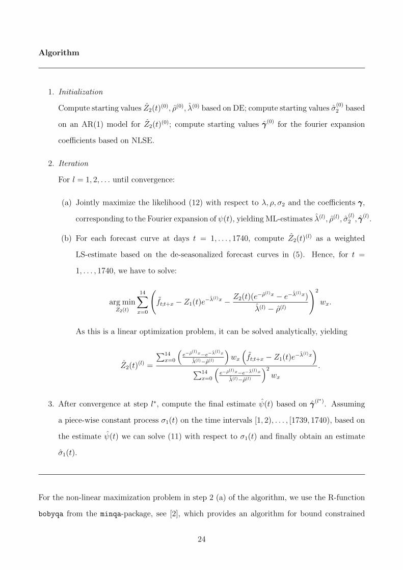
1. Initialization
Compute starting values Z2(t)(0), ρ(0), λ(0) based on DE; compute starting values σ
(0)2 based
on an AR(1) model for Z2(t)(0); compute starting values γγγ(0) for the fourier expansion
coefficients based on NLSE.
2. Iteration
For l = 1, 2, . . . until convergence:
(a) Jointly maximize the likelihood (12) with respect to λ, ρ, σ2 and the coefficients γγγ,
corresponding to the Fourier expansion of ψ(t), yielding ML-estimates λ(l), ρ(l), σ(l)2 , γγγ
(l).
(b) For each forecast curve at days t = 1, . . . , 1740, compute Z2(t)(l) as a weighted
LS-estimate based on the de-seasonalized forecast curves in (5). Hence, for t =
1, . . . , 1740, we have to solve:
arg minZ2(t)
14∑x=0
(ft;t+x − Z1(t)e
−λ(l)x − Z2(t)(e−ρ(l)x − e−λ(l)x)λ(l) − ρ(l)
)2
wx.
As this is a linear optimization problem, it can be solved analytically, yielding
Z2(t)(l) =
∑14x=0
(e−ρ
(l)x−e−λ(l)xλ(l)−ρ(l)
)wx
(ft;t+x − Z1(t)e
−λ(l)x)
∑14x=0
(e−ρ
(l)x−e−λ(l)xλ(l)−ρ(l)
)2wx
.
3. After convergence at step l∗, compute the final estimate ψ(t) based on γγγ(l∗). Assuming
a piece-wise constant process σ1(t) on the time intervals [1, 2), . . . , [1739, 1740), based on
the estimate ψ(t) we can solve (11) with respect to σ1(t) and finally obtain an estimate
σ1(t).
For the non-linear maximization problem in step 2 (a) of the algorithm, we use the R-function
bobyqa from the minqa-package, see [2], which provides an algorithm for bound constrained
24

0 20 40 60 80 100
0.0
0.2
0.4
0.6
0.8
1.0
Lag
AC
F
ACF for sq.resid AR(1)
Figure 10: Autocorrelation function of the squared AR(1)-residuals on the New York data forthe time period 1997-2012.
optimization without using derivatives. Note that, as temperature forecast are naturally less
reliable the longer the forecast period lasts, we suggest to put more weight on shorter forecast
periods and specify the following weight vector in step 2 (b) of the algorithm
w = (w0, w1, . . . , w14)ᵀ = (100, . . . , 100, 10, . . . , 10, 1, . . . , 1)ᵀ,
with w0 = . . . = w4 = 100, w5 = . . . = w9 = 10 and w10 = . . . = w14 = 1. The final estimates
for λ, ρ and σ2 yield λ(l∗) = 1.835, ρ(l
∗) = 0.107 and σ(l∗)2 = 2.713. The final fits of the forecast
curves are illustrated in Figure 11, where we show the curve estimates together with the de-
seasonalized forecast data for 9 chosen days. We can see that the fitted curves do a rather good
job within the bounds of possible curve features covered by the two-factor model (3), whereas
on several days the fitted curves corresponding to a simple AR(1) model cannot reproduce the
true forecast courses in a satisfactory way.
The final (annual) estimate for ψ(t)(l∗), which is based on the final parameter estimates γγγ(l
∗),
is plotted in Figure 12. It indicates that the standard deviation of the conditional distribution of
the temperature in (11) has its maximum in February and its minimum at the end of July. This
conforms with the findings in [10] and [19]. The corresponding piece-wise constant estimates
for σ1(t) yield values in the interval [2.584, 3.351].
25

0 2 4 6 8 10 12 14
−10
010
day 4
forecast period
0 2 4 6 8 10 12 14
−10
010
day 17
forecast period
0 2 4 6 8 10 12 14
−10
010
day 98
forecast period
0 2 4 6 8 10 12 14
−10
010
day 105
forecast period
0 2 4 6 8 10 12 14−
100
10
day 118
forecast period
0 2 4 6 8 10 12 14
−10
010
day 121
forecast period
0 2 4 6 8 10 12 14
−10
010
day 404
forecast period
0 2 4 6 8 10 12 14
−10
010
day 473
forecast period
0 2 4 6 8 10 12 14
−10
010
day 500
forecast period
Figure 11: Estimated forecast curves for the two-factor model (black solid lines) and for a simpleAR(1) model (gray dashed lines) together with de-seasonalized forecast data for 9 chosen daysfor New York.
1.4
1.6
1.8
2.0
2.2
day
ψ1(t
)
1 Jan. 1 Apr. 1 Jul. 1 Sep. 31 Dec.
Figure 12: New York final (annual) estimate ψ(t)(l∗), based on final parameter estimates γγγ(l
∗).
For Berlin, the final estimates for λ, ρ and σ2 yield λ(l∗) = 0.460, ρ(l
∗) = 0.120 and σ(l∗)2 =
0.962. The piece-wise constant estimates for σ1(t) yield values in the interval [3.016, 3.448].
Altogether, we obtain very similar results for Berlin and a comparable quality of the fitted
curves with the major difference that the standard deviation of the conditional distribution of
the temperature for Berlin has its maximum in September and its minimum at the beginning
26

of April.
4 Pricing Weather Derivatives
Weather Derivatives started to trade at the Chicago Mercantile Exchange (CME) in the late ’90s
in order to hedge weather risk. Exchange-traded temperature derivatives are futures written on
different temperature indices I(T1, T2) measured over specified periods [T1, T2] such as weeks,
months or quarters of a year, and European options written on these futures. In the following
we first derive explicit price formulas in our model for the most common futures contracts
before we perform a calibration study on the market price of risk. The question of hedging and
pricing options written on these futures is addressed in [21].
4.1 CAT, HDD and CDD futures
The most common temperature indices I(T1, T2) are: Heating Degree Day (HDD), Cooling De-
gree Day (CDD), Cumulative Averages (CAT). The temperature indices take the accumulated
average temperature over [T1, T2]:
CAT(T1, T2) =
∫ T2
T1
τudu
CDD(T1, T2) =
∫ T2
T1
max(τu − C, 0)du
HDD(T1, T2) =
∫ T2
T1
max(C − τu, 0)du ,
where τu denotes the daily average temperature. The measurement period is usually measured
in standard months or seasons and C is a threshold (typically 18C or 65F) over a period
[T1, T2]. HDD futures contracts are measured during November–April and for CDD and CAT
futures contracts the measurement period is April–November.
According to no-arbitrage theory, pricing of financial assets with the temperature as under-
lying spot price has to be done under some risk-neutral pricing measure which in our setting
can be any probability measure Q equivalent to P since the underlying cannot be traded. The
futures price FI(t, T1, T2) written on a given temperature index I(T1, T2) is chosen such that
27

the value of the futures contract equals zero at emission time t given the information Ft, i.e.
(assuming a deterministic risk-free rate for simplicity):
EQ [I(T1, T2)− FI(t, T1, T2)|Ft] = 0,
or
FI(t, T1, T2) = EQ [I(T1, T2)|Ft] , (13)
with I(T1, T2) being one of the indices CAT, HDD or CDD.
We assume that the temperature dynamics of the temperature f(t; t) = τ(t) under a risk-
neutral measure Q are given as Λ(t) + Z1(t), with
dZ1(t) = (θ1(t)σ1(t)− λZ1(t) + Z2(t)) dt+ σ1(t) dW1(t)
and
dZ2(t) = (θ2(t)σ2 − ρZ2(t)) dt+ σ2(t) dW2(t),
where dW1(t) := dW1(t) − θ1(t)dt and dW2(t) := dW2(t) − θ2(t)dt define independent Q-
Brownian motions and the market price of risk θ = (θ1, θ2) consists of some bounded determin-
istic functions. This imposes a certain restriction on the set of possible pricing measures, but
simplifies the calculations considerably. We first consider the pricing of CAT futures.
Proposition 1. For t ≤ T1, the CAT futures price F CAT(t;T1, T2) is given by
F CAT(t;T1, T2) =
∫ T2
T1
Λ(s) ds− Z1(t) lλT1,T2
(t) + Z2(t)lρT1,T2(t)− l
λT1,T2
(t)
ρ− λ
−∫ T2
t
θ1(u)σ1(u) lλu∨T1,T2(u) du
+
∫ T2
t
θ2(u)σ2lρu∨T1,T2(u)− lλu∨T1,T2(u)
ρ− λdu
28
where the function lαR,S(x) is defined by
lαR,S(x) :=e−α(S−x) − e−α(R−x)
α; α,R, S, x ∈ R ,
and x ∨ y := maxx, y. For T1 < t ≤ T2 we obtain
F CAT(t;T1, T2) =
∫ t
T1
τ(s) ds+ F CAT(t; t, T2) .
In particular, for the special case θ1(u) = θ1, θ2(u) = θ2, σ1(u) = σ1 constant on [t, T2],
Proposition 1 gives by direct computation the following CAT futures price for t ≤ T1:
F CAT(t;T1, T2) =
∫ T2
T1
Λ(s) ds− lλT1,T2(t)(Z1(t) +
Z2(t)
ρ− λ− θ1σ1
λ− θ2σ2λ(ρ− λ)
)+lρT1,T2(t)
(Z2(t)
ρ− λ− θ2σ2ρ(ρ− λ)
)+ (T2 − T1)
(θ1σ1λ
+θ2σ2ρλ
).
Proof. From (13) we obtain with I(T1, T2) the CAT index
F CAT(t;T1, T2) = EQ
[∫ T2
T1
τ(s) ds
∣∣∣∣Ft] .By Fubini’s theorem, we can rewrite
F CAT(t;T1, T2) =
∫ T2
T1
fQ(t; s) ds,
with
fQ(t; s) := EQ [τ(s)| Ft] = Λ(s) + EQ [Z1(s)| Ft] .
Now recall from (9) and (10) that for s ≥ t
Z1(s) = Z1(t)e−λ(s−t) +
∫ s
t
σ1(u)e−λ(s−u) dW1(u) (14)
+ Z2(t)
(e−ρ(s−t) − e−λ(s−t)
)λ− ρ
+
∫ s
t
∫ s
r
σ2(r)e−λ(s−u)−ρ(u−r) du dW2(r)
Rewriting (14) in terms of W1 and W2 and taking conditional expectation with respect to Q
29
gives
fQ(t; s) = Λ(s) + Z1(t)e−λ(s−t) + Z2(t)
e−ρ(s−t) − e−λ(s−t)
λ− ρ
+
∫ s
t
θ1(u)σ1(u)e−λ(s−u) du+
∫ s
t
θ2(u)σ2(u)e−ρ(s−u) − e−λ(s−u)
λ− ρdu .
Finally, using Fubini again, we can compute the CAT-futures price for t ≤ T1 as
F CAT(t;T1, T2) =
∫ T2
T1
fQ(t; s) ds
=
∫ T2
T1
Λ(s) ds− Z1(t) lλT1,T2
(t) + Z2(t)lρT1,T2(t)− l
λT1,T2
(t)
ρ− λ
−∫ T2
t
θ1(u)σ1(u) lλu∨T1,T2(u) du
+
∫ T2
t
θ2(u)σ2(u)lρu∨T1,T2(u)− lλu∨T1,T2(u)
ρ− λdu .
For T1 < t ≤ T2 we obtain
F CAT(t;T1, T2) =
∫ t
T1
τ(s) ds+ EQ
[∫ T2
t
τ(s) ds
∣∣∣∣Ft]=
∫ t
T1
τ(s) ds+ F CAT(t; t, T2) .
Next, we turn our attention to HDD and CDD futures:
Proposition 2. For t ≤ T1, the HDD futures price is given by
F HDD(t;T1, T2) =
∫ T2
T1
(C − Λ(s)− µt,s)Φ
(C − Λ(s)− µt,s
ψt,s
)
+ ψt,sφ
(C − Λ(s)− µt,s
ψt,s
)ds ,
30

and the CDD futures price is given by
F CDD(t;T1, T2) =
∫ T2
T1
(Λ(s) + µt,s − C)Φ
(Λ(s) + µt,s − C
ψt,s
)
+ ψt,sφ
(Λ(s) + µt,s − C
ψt,s
)ds ,
where Φ is the cumulative distribution function, φ the density of the standard normal distribu-
tion, and
µt,s = Z1(t)e−λ(s−t) + Z2(t)
e−ρ(s−t) − e−λ(s−t)
λ− ρ
+
∫ s
t
θ1(u)σ1(u)e−λ(s−u) du+
∫ s
t
θ2(u)σ2e−ρ(s−u) − e−λ(s−u)
λ− ρdu ,
ψ2t,s =
∫ s
t
σ21(u)e−2λ(s−u) du+
∫ s
t
(∫ s
r
σ2e−λ(s−u)−ρ(u−r) du
)2
dr .
For T1 < t ≤ T2 we obtain
F HDD(t;T1, T2) =
∫ t
T1
(C − τ(s))+ ds+ F HDD(t; t, T2) ,
F CDD(t;T1, T2) =
∫ t
T1
(τ(s)− C)+ ds+ F CDD(t; t, T2) .
Proof. The HDD futures price is given by
F HDD(t;T1, T2) = EQ
[∫ T2
T1
(C − τ(s))+ ds
∣∣∣∣Ft]=
∫ T2
T1
EQ[(C − τ(s))+
∣∣Ft] ds .Now, for a Gaussian random variable X ∼ N(µ;σ2) straight forward calculations give
EQ[(C −X)+
]= (C − µ)Φ
(C − µσ
)+ σφ
(C − µσ
),
31

where C is a constant and Φ and φ are as in Proposition 2 above.
Rewriting (14) in terms of W1 and W2 one sees that the conditional distribution of Z1(s)
given Z(t) for s ≥ t ≥ 0 under Q is
Z1(s)|Z(t) ∼ N(µt,s; ψ2t,s)
where µt,s and ψ2t,s are given in Proposition 2 above. Since τ(s) = Λ(s) + Z1(s) the result
follows.
For CDD futures prices the computations are analogue.
4.2 Calibration of the market price of risk
We now turn our attention to the calibration of the market price of risk, i.e. to the calibration of
the pricing measure used by the market to price temperature derivatives, implied by our model.
In a previous study of temperature markets by [19] it was found that the calibrated market
price of risk behaves very irregular in time, in particular when times to futures’ maturities
become short. In that study, the temperature is modeled by a CAR(3) model (continuous
time autoregressive of order 3) and the information available to the market is modeled by the
filtration generated by the temperature.
However, as argued in the introduction, we believe that at least parts of the irregular
behavior of the market price of risk in [19] is not due to irregular risk pricing of the market
but due to a misspecification of the model that is used to calibrate risk prices: forward looking
information about the temperature available to the market is not taken into account in the
information modeling. Obviously, when the information available to the market is assumed to
be generated only by the past temperature, substantial amounts of forward looking information
available to the market is not taken care of in [9] and [19].
In our approach we include, at least essential parts of, available forward looking information
by specifying a model for the complete forecast curve and the intention of this section is now to
estimate the market price of risk structure implied by our model approach and to compare it to
32
the market price of risk obtained without meteorological forecast information. To this end, we
calibrate model implied futures prices to the market and proceed as follows. For simplicity, we
assume the market prices of risk θ1(u) = θ1 and θ2(u) = θ2 to be constant. Then Proposition
2 yields by direct computations:
µt,s = Z1(t)e−λ(s−t) + Z2(t)
e−ρ(s−t) − e−λ(s−t)
λ− ρ
+ θ1
∫ s
t
σ1(u)e−λ(s−u) du+θ2σ2λ− ρ
1− e−ρ(s−t)
ρ+
1− e−λ(s−t)
λ
.
and
ψ2t,s =
∫ s
t
σ21(u)e−2λ(s−u) du
+σ22
(λ− ρ)2
1− e−2ρ(s−t)
2ρ+
1− e−2λ(s−t)
2λ− 2(1− e−(ρ+λ)(s−t))
ρ+ λ
.
We got access to prices for 7 CAT futures contracts for the region of Berlin-Tempelhof
airport from the Chicago Mercantile Exchange (CME) traded within the time period 20081229-
20091031 and measurement period (April - Nov) as well as prices of 45 HDD and CDD futures
contracts for the region of New York-JFK airport5 within the time period 20081229-20120330.
In the following we use the formulas from Proposition 2 to compute the course of the market
price of risk, based on the model parameter estimates derived in Section 3.2. For comparison, we
also compute the market prices of risk based on a simple AR(1) model, which does not include
any meteorological forecast information and is solely estimated on past temperatures. Note here
that as the European CAT futures market is hardly liquid and thus the CAT futures price time
series for Berlin are mostly constant, even within the delivery period, also the corresponding
courses of the market price of risk θ1 are basically constant lines, with some spikes close to
delivery. Hence, we restrict our analysis in the following on the New York data, in particular
on New York HDD futures prices.
For both methods we successively derive the market price of risk θ1(t) for all days t where
futures prices of the considered HDD were available to us, by solving the equality for the HDD
5The temperature futures were obtained from Bloomberg.
33

futures price F HDD(t;T1, T2) from Proposition 2 with respect to θ1. For the AR(1) approach we
simply set both Z2(t) and σ22 equal to zero.
At this point we want to recall the data inconsistencies of temperature and forecasts al-
ready mentioned in Footnote 1 and in Section 2.1 which are a possible error source concerning
the results of our market price of risk calibrations. These inconsistencies don’t allow to fully
exploit the forward looking information contained in meteorological forecasts. So the perfor-
mance of our model parameter estimates and hence, the quality of our market price of risk
calibrations could potentially be considerably improved, if the forecast data would correspond
to the temperature data.
In Figure 13 and Figure 14 we show the results for a selection of New York HDD futures
based on our two-factor model from (3) (black solid line) and based on the AR(1) approach
(gray dashed line). We find that in all investigated scenarios the courses of the market prices
of risk are generally similar for both used methods and at a first glance no major differences
are visible. To make the courses comparable we have standardized them, always taking the
first available day of the futures price time series as the reference point. For both methods, the
market price of risk is quite steady before the delivery period begins, but then becomes more
and more turbulent when getting close to delivery.
But if we have a closer look on the total relative variation in the courses, corresponding to
a given series of HDD futures prices on a time interval [t, T2], i.e.
TV :=
T2−1∑s=t
|θ1(s+ 1)− θ1(s)||θ1(s)|
,
we find that the market prices of risk based on our two-factor model behave more regular than
those based on the AR(1) approach, both on the whole time interval and during the delivery
period, compare Table 2 and Table 3. Though the differences might not seem to be crucial,
we still can observe the trend that a model accounting for forward looking information leads
to more regular market prices of risk. In particular, the quality of the incorporated forward
looking information in the two-factor model could be probably considerably improved, if the
data inconsistencies mentioned above could be eliminated.
34

−3.
0−
2.0
−1.
00.
00.
5
MPR for HDD No. 1
time
MP
R
Dec 30 Jan 06 Jan 13 Jan 20 Jan 27
−2.
0−
1.5
−1.
0−
0.5
0.0
MPR for HDD No. 14
time
MP
R
Mar May Jul Sep Nov
Figure 13: Standardized market price of risk courses for a selection of New York HDD futuresprices based on the two-factor model from (3) (black solid line) and on an AR(1) model (graydashed line); the start of the delivery period is indicated by the dashed vertical line.
35

−1.
0−
0.8
−0.
6−
0.4
−0.
20.
0
MPR for HDD No. 16
time
MP
R
May Jul Sep Nov Jan Mar
−1.
0−
0.8
−0.
6−
0.4
−0.
20.
0
MPR for HDD No. 29
time
MP
R
Sep Jan May Sep Jan
Figure 14: Standardized market price of risk courses for a selection of New York HDD futuresprices based on the two-factor model from (3) (black solid line) and on an AR(1) model (graydashed line); the start of the delivery period is indicated by the dashed vertical line.
36

HDD No. 1 14 16 29TVAR(1) 4.93 25.60 11.13 9.26TV2-factor 3.86 24.51 10.17 8.22
Table 2: Difference in total relative variation between the two-factor and AR(1) model for aselection of New York HDD futures.
HDD No. 1 14 16 29TVAR(1) 4.62 19.07 4.11 4.91TV2-factor 3.59 18.02 3.21 3.91
Table 3: Difference in total relative variation between the two-factor and AR(1) model for aselection of New York HDD futures (only in the delivery period).
5 Conclusion
We propose a consistent two-factor model for pricing temperature derivatives that incorporates
the forward looking information available in the market by specifying a reduced model for the
complete temperature forecast curve in addition to the evolution of the temperature. The
two factors describing the tilting or bending of the curves reflect accurately the stylized facts
of temperature and temperature forecast in the short end. The two-factor model allows for
factors with mean-reversion to a stochastic mean level. We find that the market prices of risk,
calibrated from CME temperature derivatives, based on our two-factor models behave more
regular than those based on an AR(1)-Ornstein-Uhlenbeck approach, both in and out of the
measurement period.
Acknowledgement
The financial support from the Deutsche Forschungsgemeinschaft via SFB 649 “Okonomisches
Risiko”, Humboldt-Universitat zu Berlin is gratefully acknowledged.
37

References
[1] Alaton, P., Djehiche, B., and Stillberger, D. (2002). On modelling and pricing weather
derivatives. Appl. Math. Finance, 9(1):1–20.
[2] Bates, D., Mullen, K. M., Nash, J. C., and Varadhan, R. (2012). minqa: Derivative-free
optimization algorithms by quadratic approximation. R package version 1.2.1.
[3] Bates, D. M. and Watts, D. G. (1988). Nonlinear Regression Analysis and Its Applications.
Wiley.
[4] Bellman, R. E. (1961). Adaptive Control Processes: A Guided Tour. Princeton University
Press, Princeton.
[5] Benth, F., Biegler-Konig, R., and Kiesel, R. (2013). An empirical study of the information
premium on electricity markets. Energy Economics, 36:55–77.
[6] Benth, F. and Meyer-Brandis, T. (2009). The information premium for non-storable com-
modities. Journal of Energy Market, 2.
[7] Benth, F. E. and Benth, S. (2011). Weather derivatives and stochastic modelling of tem-
perature. International Journal of Stochastic Analysis, 2011:1–21.
[8] Benth, F. E., Cartea, A., and Kiesel, R. (2008). Pricing forward contracts in power markets
by the certainty equivalence principle: Explaining the sign of the market risk premium.
Journal of Banking and Finance, 32(10):2006–2021.
[9] Benth, F. E. and Saltyte Benth, J. (2012). Modeling and Pricing in Financial Markets for
Weather Derivatives. Band 17, Advanced Series on Statistical Science and Applied Proba-
bility, World Scientific Publishing Company Incorporated.
[10] Benth, F. E., Saltyte Benth, J., and Koekebakker, S. (2007). Putting a price on tempera-
ture. Scandinavian Journal of Statistics, 12(1):53–85.
[11] Brockett, P., Wang, M., Yang, C., and Zou, H. (2006). Portfolio effects and valuation of
weather derivatives. Financial Review, 41(1):55–76.
38
[12] Campbell, S. and Diebold, F. (2005). Weather forecasting for weather derivatives. Journal
of American Statistical Association, 100(469):6–16.
[13] Cao, M. and Wei, J. (2004). Weather derivatives valuation and market price of weather
risk. The Journal of Future Markets, 24(11):1065–1089.
[14] Dorfleitner, G. and Wimmer, M. (2010). The pricing of temperature futures at the chicago
mercantile exchange. Journal of Banking and Finance, 34(6):1360–1370.
[15] Filipovic, D. (1999). A note on the nelson-siegel family. Mathematical Finance, 9:349–359.
[16] Gilli, M., Große, S., and Schumann, E. (2010). Calibrating the Nelson–Siegel–Svensson
model. COMISEF Working Paper Series No. 31. available from http://comisef.eu/?q=
working_papers.
[17] Gilli, M., Maringer, D., and Schumann, E. (2011). Numerical Methods and Optimization
in Finance. Academic Press.
[18] Hardle, W., Lopez-Cabrera, B., and Ritter, M. (2012). Forecast based pricing of weather
derivatives. SFB 649 Discussion Paper 2012-027.
[19] Hardle, W. K. and Lopez-Cabrera, B. (2012). The implied market price of weather risk.
Applied Mathematical Finance, 19(1):59–95.
[20] Hardle, W. K., Lopez-Cabrera, B., Okhrin, O., and Wang, W. (2011). Localizing tempera-
ture risk. SFB 649 Discussion Paper 2011-01, Humboldt- Universitat zu Berlin. 2nd Revision
in Journal of Econometrics.
[21] Hell, P., Meyer-Brandis, T., and Rheinlander, T. (2012). Consistent factor models for tem-
perature markets. International Journal of Theoretical and Applied Finance, 15(4):1250027–
1–1250027–24.
[22] Huang-Hsi, H., Yung-Ming, S., and Pei-Syun, L. (2008). Hdd and cdd option pricing with
market price of weather risk for taiwan. The Journal of Future Markets, 28(8):790–814.
39
[23] Jewson, S. and Brix, A. (2005). Weather Derivative Valuation. Cambridge University
Press, Cambridge.
[24] Nelson, C. R. and Siegel, A. F. (1987). Parsimonious modeling of yield curves. The Journal
of Business, 60(4):473–489.
[25] R Core Team (2013). R: A Language and Environment for Statistical Computing. R
Foundation for Statistical Computing, Vienna, Austria.
[26] Ramsay, J. O. and Silverman, B. W. (2005). Functional Data Analysis. Springer, New
York, 2nd edition.
[27] Richards, T., Manfredo, M., and Sanders, D. (2004). Pricing weather derivatives. American
Journal of Agricultural Economics, 86(4):1005–1017.
[28] Ritter, M., Musshoff, O., and Odening, M. (2011). Meteorological forecasts and the pricing
of temperature futures. Journal of Derivatives, 19.
[29] Shang, H. L. (2013). A survey of functional principal component analysis. Advances in
Statistical Analysis.
[30] Viviani, R., Gron, G., and Spitzer, M. (2005). Functional principal component analysis of
fMRI data. Human Brain Mapping, 24:109–129.
[31] Yoo, S. (2004). Weather derivatives and seasonal forecast. Asia-Pacific Journal of Finan-
cial Studies, pages 213–246.
40