Evaluating Factor Pricing Models

Using High Frequency Panels1

Yoosoon Chang2, Hwagyun Kim3 and Joon Y. Park4

Abstract

This paper develops a new framework and statistical tools to analyze stock re-turns using high frequency data. We consider a continuous-time multi-factormodel via a continuous-time multivariate regression model incorporating real-istic empirical features, such as persistent stochastic volatilities with leverageeffects. We find that conventional regression approach often leads to misleadingand inconsistent test results. We overcome this by using samples collected atrandom intervals, which are set by the clock running inversely proportional tothe market volatility. We find that the size factor has difficulty in explaining thesize-based portfolios, while the book-to-market factor is a valid pricing factor.

This Version: August, 2010JEL Classification: C33, C12, C13

Key words and phrases: panel, high-frequency, time change, realized variance, Fame-Frenchregression.

1We thank the participants at 2010 International Symposium on Financial Engineering and Risk Man-agement, 2009 Panel Data Conference, 2009 SETA Meeting, 2009 Meeting of Midwest Econometrics Group,and the seminar participants at Cowles Foundation at Yale, Louisiana State University, Michigan State Uni-versity, Ohio State University, Purdue, Rochester, Seoul National University, Soveriges Riksbank, StatisticalColloquium at Indianan and Vanderbilt for their helpful comments. We are also grateful to Yongok Choi andHyosung Yeo for excellent research assistance. Chang gratefully acknowledges the financial support fromthe NSF under Grant SES-0453069/0730152.

2Corresponding author. Address correspondence to Yoosoon Chang, Department of Economics, IndianaUniversity, Wylie Hall Rm 105, 100 S. Woodlawn, Bloomington IN 47401-7104, or to yoosoon@indiana.edu.

3Department of Finance, Mays Business School, Texas A&M University4Department of Economics, Indiana University and Sungkyunkwan University

1. Introduction

The empirical anomalies related to the Capital Asset Pricing Model (CAPM), typified bythe size, value, and momentum effects, lie at the center of multi-factor asset pricing models.Especially, the model by Fama and French (1992, 1993) incorporates the excess returnson two portfolios capturing the size and value premiums as the additional factors. Theyestimated and tested this three-factor model using twenty-five equity returns from portfoliossorted by stocks’ sizes and book-to-market ratios. The research in empirical finance hasbeen focusing on multi-factor asset pricing models since then, and mainly geared towardidentifying asset pricing anomalies, thereby new pricing factors. Finding a new factortypically begins with grouping stocks by a characteristic, such as size, book to market ratio,or past return performances. Then, econometric analyses follow, verifying if there existsignificant, abnormal returns not explained by the incumbent pricing factors, and testing ifa new model embedding an additional factor made from the anomaly variable is rejected.That is, empirical asset pricing involves the construction of panel data sets of returns, andthe ensuing statistical investigation of those data series with some economic restrictions.

In the paper, we develop a new framework and a new set of statistical tools for high fre-quency panels and use them to reexamine Fama-French regressions.5 Our approach utilizessome recent econometric research on models with high frequency observations. Fama-Frenchregressions have still been analyzed largely within the classical regression framework. Thereare at least two dimensions that we may look into for a new opportunity using our approach.First, asset return data sets are available at several different frequencies, e.g., daily, monthlyand yearly. However, very few attempts have been made to address the issue of how to usethese data sets provided at multiple frequencies. In modern financial markets, informationflows almost in real time and assets are traded at high frequencies. Thus, a valid assetpricing model under the premise of well-functioning markets must delineate relationshipsbetween asset returns and pricing factors at the (high) frequency of market clearing. Thisimplies that a proper integration of higher frequency models is needed to accurately estimateand test asset pricing models at lower frequencies.

Second, financial asset returns used in Fama-French regressions are extremely volatileat high frequencies. This excessive volatility introduces too much noise to make it mean-ingful to run regressions at high frequencies. Moreover, virtually all asset returns showa strong evidence of time-varying and stochastic volatilities, and of leverage effects. Thetime-varying and stochastic volatilities would have only a second-order effect, if they areasymptotically stationary. Unfortunately, however, all empirical researches reported in theliterature unanimously and unambiguously find that they are nonstationary, which is at-tributable to structural breaks, switching regimes and/or near-unit roots,6 and endogenous

5The empirical asset pricing literature often uses the term, Fama-French regressions to refer to multi-factor pricing models containing size or firm distress factors. For instance, a model including a momentumfactor in addition to the three Fama-French factors is called, four-factor Fama-French model. See Carhart(1997) for details. Following this convention, we regard Fama-French regressions as multi-factor models incontrast to the CAPM.

6The reader is referred to Jacquier, Polson and Ross (1994, 2004), So, Lam and Li (1998) and Kim, Lee,and Park (2009) for the evidence of nonstationarity in stock return volatilities.

1

due to leverage effects. As shown in Chung and Park (2007), the nonstationary volatilitiesgenerally affect the limit distributions and invalidate the standard tests.7 The negligenceor misspecification of the time-varying and stochastic volatilities would therefore have afirst-order effect. The presence of leverage effects introduces endogeneity in volatilities,which makes it more complicated to deal with the nonstationarity of volatilities.8 It wouldcertainly be a challenging problem to statistically analyze regressions with endogenous non-stationary stochastic volatilities.

To analyze Fama-French regressions, we derive a continuous time multifactor pricingmodel and consider the corresponding panel regression. Our model is very general in thesense that it allows for time-varying and stochastic volatilities, which are both nonsta-tionary and endogenous. The error term is just given as a general martingale differential,consisting of two components, namely, the common component and the idiosyncratic com-ponent, which are independent of each other. The common component is specified as havingvolatility driven by the market, but otherwise it is entirely unrestricted. We may of coursepermit the presence of endogenous nonstationarity in the volatility process of the com-mon component. On the other hand, the idiosyncratic component is only assumed to becross-sectionally independent and have an asymptotically stationary volatility process. Ourspecification for the idiosyncratic component is therefore also very flexible and unrestrictive.In fact, the only meaningful restriction imposed on our error component model is that itsnonstationary volatility component is generated exclusively by the market. This implies inparticular that only the market risk is non-diversifiable over time.9 Our specification of theerror components is justified both theoretically and empirically in the paper.

For the statistical analysis of our model, we develop a new methodology relying on thesampling at random intervals in lieu of fixed intervals, and using the realized variance mea-sure at a higher frequency to estimate the variance of the resulting sample. Our approachexploits a well known theorem in the theory of stochastic processes, due to Dambis, Dubinsand Schwarz, which is often referred to as the DDS theorem.10 It implies that any realiza-tion from a continuous martingale can be regarded as a realization from Brownian motion ifit is read using the clock running at a speed inversely proportional to its quadratic variation.At least on its continuous part, a martingale generated with an arbitrary volatility processcan therefore be converted into a Brownian motion simply by a time change in sampling.Consequently, general martingale differentials now become Brownian differentials, which areindependent and identically distributed normals.11 The DDS theorem is not directly appli-cable if the error process is discountinuous and has jumps. However, our approach remainsto be valid asymptotically also in this case, as long as jumps are exogenous and occurs

7They also show that the regressions may even become spurious in case that the nonstationary volatilitiesare excessive.

8For more details of the leverage effects, the reader is referred to Harvey and Shepard (1996), Jacquier,Polson and Ross (2004), Yu (2005) and Kim, Lee, and Park (2009).

9As shown in Park (2002), the usual law of large numbers does not hold in the presence of nonstationaryvolatility.

10Readers are referred to, e.g., Revuz and Yor (1994) for more details about the DDS theorem.11For the application of this approach in the univariate setup, see Phillips and Yu (2005), and Andersen,

Bollerslev and Dobrev (2007). It has been more systematically and rigorously developed recently by Park(2009).

2

intermittently. This is because our statistical theory only requires asymptotic normality,not normality in finite samples, of the regression errors after time change.

For our model, we may use the market volatility to set the required random samplingintervals. This is because only the market volatility drives the endogenous nonstationarityin our error component model. As long as the volatility in the common component is takencare of by sampling at proper random intervals, the errors become asymptotically normal.The variance of the errors collected at the random intervals is also determined by theidiosyncratic component, but its volatility is asymptotically stationary as in the standardregression model. Moreover, the error variance can be estimated readily by the realizedvariance obtained from higher frequency observations available at each random interval.Our methodology therefore utilizes observations at both high and low frequencies. We useobservations at a high frequency to set the random sampling intervals, and to estimatethe variance of collected samples. On the other hand, are used samples collected at a lowfrequency to analyze the main regressions. They are analyzed at a low frequency to avoiddistortions caused by excessive volatilities existing at high frequency observations. At thesame time, however, we do not discard the available observations at the higher frequency,i.e., we also use them to deal with time-varying and stochastic volatilities in observationscollected at a low frequency.

With this new econometric methodology in hand, we revisit the classic issues in empiricalasset pricing. We estimate and test the CAPM and various multi-factor Fama-French modelson five data sets of daily equity returns, which consist of three sets of decile portfolios sortedrespectively by size, book-to-market ratio (B/M), and past performances (momentum); aset of twenty five portfolios sorted by size and B/M; and a set of thirty portfolios fromdifferent industries. For our random time regressions, we select the sampling intervals usingthe realized variance series of the daily excess market returns by setting the realized varianceover each random sampling interval at the level comparable to the average realized varianceof the monthly excess market returns. In the paper, we compare the results from our randomtime regressions with those from fixed time regressions using monthly observations.

We find that conventional regressions on fixed time intervals yield confusing test results.Specifically, with the fixed time sampling, we cannot reject the CAPM on the size portfoliosand the B/M portfolios even if the estimated market betas cannot explain the higher riskpremium generated by small size or high book-to-market ratio.12 This result is inconsistentwith the vast amount of literature on the existence of size and value premia of stock returns.Furthermore, when we incorporate the B/M or the size factor into the CAPM regression oneach of the corresponding data sets, the fixed-time monthly OLS regressions cannot rejectthe two-factor models with even higher p-values, stating that one cannot statistically rejectneither CAPM nor respective two-factor models on those portfolios. However, when allthree factors are included, i.e., when the Fama-French 3-factor model is used for estimationon 25 portfolios sorted both by size and B/M, we have a flat rejection of the model. That is,this conventional method ignoring time-varying volatilities gives logically inconsistent testresults.

12For the industry portfolios, the CAPM is not rejected either. However, it is rejected in case of themomentum portfolios.

3

Meanwhile, our random sampling approach based on time change decisively rejects theCAPM, reproducing the asset pricing anomalies compatible with the previous literature.Then, we estimate the two-factor models on each corresponding portfolios to find that theB/M factor is indeed a valid pricing factor explaining variations in stock returns due todifferent book-to-market ratios. However, the test result shows that the size factor is notsufficient to capture the cross sections of stock returns. Consistent with these findings,the three-factor model on 25 portfolios is rejected, and it turns out to be closely relatedto the small firm effect. Therefore, the random sampling approach offers a reliable andcorrect statistical method to estimate and test multi-factor asset pricing models with highfrequency data. Related, we find that the estimates of beta coefficients in most cases studiedare not critically different across the two econometric procedures. Thus, their differencesseem to come mainly from the estimates of constant terms and variance-covariance matrixof residual terms, implying the importance of properly treating highly persistent stochasticvolatilities of residual terms.

Finally, when applied to the industry portfolios, we again obtain similar results: theconventional method cannot reject the CAPM, despite significant deviations of abnormalreturns from zero, resulting in the rejection of the CAPM in the random sampling case.The main reason for the rejection turns out to be the portfolio returns from consumerproduct companies. This only prevails in the random sampling case. We find that thereturns from the consumer goods industry help explain the size effect of the Fama-Frenchportfolios, especially the returns of the micro cap, growth firms. In sum, our empiricalresults coherently show that by appropriately handling stochastic volatilities, our methodprovides an accurate statistical procedure for both estimation and testing, without losingthe attractive features of OLS regression. Thus, the good news that we want to conveyis that empirical researchers can run OLS regressions of multi-factor pricing models usingdata sets in any (especially high) frequencies and accurately test the adequacy of thosemodels, provided that the persistent market stochastic volatilities are well treated usingour time-change method. Another related point to be made from our empirical result isthat we still need valid pricing factors to explain cross sectional behaviors of stock returnsvia factor models.

The rest of the paper is organized as follows. In Section 2, we develop a continuous timemulti-factor model of asset returns with stochastic volatilities and propose a panel regressionmodel based on our theoretical framework. Section 3 presents a statistical procedure toanalyze our model and asymptotic theories. In so doing, we also provide a statisticaltoolkit necessary for our empirical analysis. Section 4 describes the data sets used in ourempirical analysis and provide empirical evidence for various specifications of our model. Wethen employ our new methodology to reexamine the CAPM and Fama-French regressionsin Section 5, where empirical results from our analysis of Fama-French regressions aresummarized and compared with other results reported in the literature. Section 6 concludesthe paper. Useful lemmas and their proofs and the proofs of the main theorems are collectedin Mathematical Appendix.

4

2. The Model and Assumptions

2.1 Theoretical Background

In this section, we derive a continuous-time beta model of asset returns on which our studyof Fama-French regressions will be based. For the derivation of our model, we let π be thestate price density given by

dπt

πt= υtdt +

J∑

j=1

τjtdVjt, (1)

where υ and (τj) are respectively drift and volatility processes, and (Vj) are independentBrownian motions. Subsequently, we specify the price process (Pi) of security i = 1, . . . , Ias

dPit

Pit= µitdt + σt

J∑

j=1

κijdVjt +K∑

k=1

λikdWk

+ ωitdZit, (2)

where (µi) and (σ, ωi) are drift and volatility processes, (κij , λik) are nonrandom coefficients,and (Zi) and (Wk) are independent Brownian motions. Throughout the paper, we assumethat

Assumption 2.1 (Zi), (Vj) and (Wk) are independent Brownian motions such that(ωi, Zi) and (σ, Vj ,Wk) are independent of each other, and such that (Wk) are Brownianmotions independent of (Vj) conditional on σ.

State price density π is a process which makes (πPi) a martingale for all i = 1, . . . , I. It iswell known since Harrison and Kreps (1979) that the existence of a state price density impliesno arbitrage in the asset market. Throughout this section, we regard the instantaneousreturns of a risky asset (dPi/Pi) as the total returns from trading gains and the dividendspaid between t and t + dt.

The drift term (µi) in (2) measures the risk return trade off, which will be determinedbelow. For the specification of the diffusion term in (2), we introduce the component withthe common volatility σ, as well as the component representing the idiosyncratic volatility(ωi) specific to asset i. The common volatility component is then further divided intotwo components, the one involving (Vj) and the other consisting only of (Wk) that areindependent of (Vj). In total, we have three terms describing the stochastic evolutionof (dPi/Pi). The first term involving (Vj) results from the covariations with the stateprice density π, and is therefore closely related to the pricing factor. The coefficient (κij)measures the proportionality of the risk of security i relative to that of (Vj). Meanwhile,the second and third terms including (Wk) and (Zi) have no bearing on π, and are notused to pin down the conditional mean component (µi) in (2). Instead, (Wk) and (Zi) areviewed as fluctuations related to the part of a firm’s cash flows which makes volatile thedividend process, and in turn, the gross return process. Alluded is that the remainder ofthe firms’ cash flows will matter for valuing the equity of these firms and these are already

5

included in the first part (σκijdVj).13 What (Wk) and (Zi) capture, we believe, are thefluctuations of the dividends of these firms which do not affect investors’ discount factorsfor pricing purposes. This is a sensible assumption based on the empirical evidence thatrealized sample paths of firms’ dividends are much more volatile than those of aggregateconsumption growth or other macroeconomic variables, which ought to be associated withthe state price density process.14 Our setup states that if individual assets’ payoffs are notcorrelated with the state-price density π, there will be no risk-return trade-off, which willbe reflected via the terms in (µi) despite the volatility of asset returns.

Now we introduce pricing factors (Qj), which we specify as

dQjt

Qjt= νjtdt + ρjσtdVjt (3)

for j = 1, 2, ..., J , where in particular (νj) are drift processes and (ρj) are nonrandomcoefficients. In our specification, (Qj) can be understood as the price of a portfolio made outof individual assets so that only systematic diffusion part relevant for pricing will remain.15

For instance, we can think of the price of a portfolio with a long position for small firms (orhigh book-to-market ratio) and a short position for large firms (or low book-to-market ratio)as a factor. In the similar context, the first factor Q1 is set to be the market factor with theunit corresponding coefficient of ρ’s, i.e., ρ1 = 1.16 The subsequent derivation of our modeldepends crucially on the existence of a common volatility movement σ, especially withconstant proportionality of risk for all assets. When the assumption of constant proportionis relaxed, we obtain a conditional beta representation, leading to conditional factor models.With some additional assumptions on the structure of betas, we may also consider suchmodels as in Ang and Kristensen (2009). However, given our emphasis on the Fama-Frenchregressions on stock returns, we do not pursue this route in this paper.

We derive our main formula by invoking the definition of the state price density. Underno arbitrage condition, we may easily deduce from (1), (2) and (3) that

µit = −υt −J∑

j=1

κijσtτjt

νjt = −υt − ρjσtτjt (4)

holds for i = 1, . . . , I and j = 1, . . . , J . Note that the left-hand-side of the first equation in(4) represents a conditional mean return for holding security i. If κij = 0 for all j, i.e., thereis no risk for this asset’s payoffs, then −υt is the resultant return process, thereby it standsfor the instantaneously riskless rate denoted as rf

t . As mentioned earlier, this equation13It is an important task to quantify the relative contributions to explaining systematic return variations

between the discount factor risk and cash flow risk. However, it is beyond the scope of our paper.14Alternatively, one may consider that the asset market is incomplete in the sense that a source of shock

(Wk) is either not priced or priced with a significantly downward bias via the conditional mean component.15It is possible to allow for the presence of non-pricing factors (Wk) we introduced in (2). This will,

however, make the Fama-French OLS regressions invalid, as we will explain later.16That is, we regard the market as the asset that includes only the systematic component for pricing with

the reference value of 1 for the beta, which will be introduced later.

6

describes the important characteristics of risk-return trade-off via conditional covariationbetween an asset’s return and the discount factor π. Upon setting υt = −rf

t , it followsimmediately from (4) that

µit − rft =

J∑

j=1

βij(νjt − rft ), (5)

where βij = κij/ρj for i = 1, . . . , I and j = 1, . . . , J .Now we have from (2), (3) and (5) that

dYit

Yit= αi +

J∑

j=1

βijdXjt

Xjt+ dUit (6)

with αi = 0 and

dUit = σt

K∑

k=1

λikdWkt + ωitdZit, (7)

if we define

dYit

Yit=

dPit

Pit− rf

t dt

dXjt

Xjt=

dQjt

Qjt− rf

t dt,

for i = 1, . . . , I and j = 1, . . . , J .Our subsequent empirical analysis will be based on the model given by (6) and (7).

Imposing the loadings of all other factors than the market factor to zero gives us theconventional CAPM regression in continuous time. One important restriction given in thismodel is that the constant coefficient αi is not present for all i in our theoretical models.Since we only use excess returns for both factors and test assets, αi = 0 must hold forall i. In this vein, we call α the pricing errors throughout the paper, where we writeα = (α1, . . . , αI)′. Testing the hypothesis of α = 0 has been a focal point of empirical assetpricing literature. Unlike the conventional discrete-time CAPM or multi-factor models,note that our continuous time model offers an error structure derived from the underlyingasset pricing model. Therefore, the estimation of the model (6) and the related statisticalinference require further elaboration. To tackle this, we develop our econometric methodand procedure below.17

2.2 Regression Formulation

Our model (6) is formulated as an instantaneous regression, where both the regressand andregressors are measured over an infinitesimal time interval. The regressions for observations

17In our model, the error process U is assumed to be a continuous process. However, the assumption canbe relaxed and we may allow for the presence of jumps. This will be discussed in the next section.

7

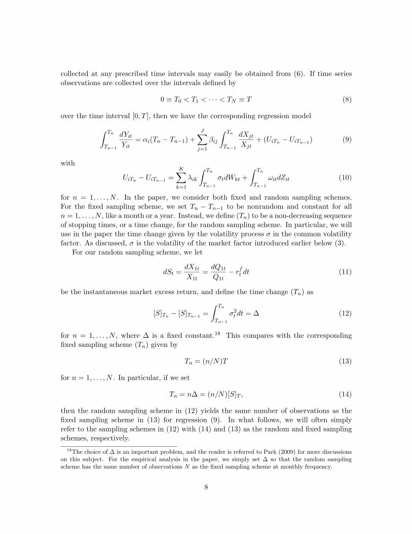
collected at any prescribed time intervals may easily be obtained from (6). If time seriesobservations are collected over the intervals defined by

0 ≡ T0 < T1 < · · · < TN ≡ T (8)

over the time interval [0, T ], then we have the corresponding regression model

∫ Tn

Tn−1

dYit

Yit= αi(Tn − Tn−1) +

J∑

j=1

βij

∫ Tn

Tn−1

dXjt

Xjt+ (UiTn − UiTn−1) (9)

with

UiTn − UiTn−1 =K∑

k=1

λik

∫ Tn

Tn−1

σtdWkt +∫ Tn

Tn−1

ωitdZit (10)

for n = 1, . . . , N . In the paper, we consider both fixed and random sampling schemes.For the fixed sampling scheme, we set Tn − Tn−1 to be nonrandom and constant for alln = 1, . . . , N , like a month or a year. Instead, we define (Tn) to be a non-decreasing sequenceof stopping times, or a time change, for the random sampling scheme. In particular, we willuse in the paper the time change given by the volatility process σ in the common volatilityfactor. As discussed, σ is the volatility of the market factor introduced earlier below (3).

For our random sampling scheme, we let

dSt =dX1t

X1t=

dQ1t

Q1t− rf

t dt (11)

be the instantaneous market excess return, and define the time change (Tn) as

[S]Tn − [S]Tn−1 =∫ Tn

Tn−1

σ2t dt = ∆ (12)

for n = 1, . . . , N , where ∆ is a fixed constant.18 This compares with the correspondingfixed sampling scheme (Tn) given by

Tn = (n/N)T (13)

for n = 1, . . . , N . In particular, if we set

Tn = n∆ = (n/N)[S]T , (14)

then the random sampling scheme in (12) yields the same number of observations as thefixed sampling scheme in (13) for regression (9). In what follows, we will often simplyrefer to the sampling schemes in (12) with (14) and (13) as the random and fixed samplingschemes, respectively.

18The choice of ∆ is an important problem, and the reader is referred to Park (2009) for more discussionson this subject. For the empirical analysis in the paper, we simply set ∆ so that the random samplingscheme has the same number of observations N as the fixed sampling scheme at monthly frequency.

8

The motivation for our random sampling scheme (12) is to effectively deal with theendogenous nonstationarity of market volatility σ in the common error component of (10).It is well known and clearly demonstrated in the literature that the market volatility has anautoregressive root that is very close to unity. Also, its leverage effect on the market excessreturn is quite strongly negative. The reader is referred to Jacquier, Polson and Rossi(1994, 2004) and Kim, Lee and Park (2009) for more discussions on the nonstationarityand leverage effect of market volatility. In this situation, the usual law of large numbersand central limit theory do not hold and hence the usual chi-square tests for inference inregression (9) are invalid as shown in e.g., Park (2002). This poses a serious problem inanalyzing Fama-French regressions. Under the random sampling scheme, however, we have

∫ Tn

Tn−1

σtdWkt =d N(0, ∆) (15)

for all n = 1, . . . , N and k = 1, . . . ,K, and that they are independent of each other. Hereand elsewhere in the paper, we use N to signify normal distribution. This is due to a theoremby Dambis, Dubins and Schwarz, which will be called the DDS theorem in the paper. Ofcourse, the normality in (15) only applies to the random sampling scheme.

The idiosyncratic error component of (10) is expected to behave much more nicely.Under Assumption 2.1, (

∫ Tn

Tn−1ωitdZit) becomes independent across i and has variance

E

(∫ Tn

Tn−1

ωitdZit

)2

= E

(∫ Tn

Tn−1

ω2itdt

)(16)

for each i = 1, . . . , I. In what follows, we assume

Assumption 2.2 For all i = 1, . . . , I, we have

1N

N∑

n=1

∫ Tn

Tn−1

ω2itdt →p $2

i

as N →∞, for some $2i > 0.

Assumption 2.2 is not stringent and should be satisfied widely. It holds under mild reg-ularity conditions if, for instance, the volatilities generated by the idiosyncratic compo-nent over the random sampling intervals are asymptotically stationary. In particular, thepresence of nonstationarity is not allowed in the idiosyncratic error component of ourmodel. Note that we still permit endogeneity in (ωi). In the special case where the id-iosyncratic volatilities (ωi) are independent of the driving Brownian motions (Zi), we have∫ Tn

Tn−1ωitdZit =d MN

(0,

∫ Tn

Tn−1ω2

itdt), where MN denotes mixed normal distribution.19

19This will be the case, if there is no leverage effect on the asset return generated from the idiosyncraticerror component.

9

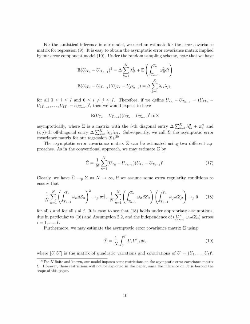
For the statistical inference in our model, we need an estimate for the error covariancematrix for regression (9). It is easy to obtain the asymptotic error covariance matrix impliedby our error component model (10). Under the random sampling scheme, note that we have

E(UiTn − UiTn−1)2 = ∆

K∑

k=1

λ2ik + E

(∫ Tn

Tn−1

ω2itdt

)

E(UiTn − UiTn−1)(UjTn − UjTn−1) = ∆K∑

k=1

λikλjk

for all 0 ≤ i ≤ I and 0 ≤ i 6= j ≤ I. Therefore, if we define UTn − UTn−1 = (U1Tn −U1Tn−1 , . . . , UITn − UITn−1)

′, then we would expect to have

E(UTn − UTn−1)(UTn − UTn−1)′ ≈ Σ

asymptotically, where Σ is a matrix with the i-th diagonal entry ∆∑K

k=1 λ2ik + $2

i and(i, j)-th off-diagonal entry ∆

∑Kk=1 λikλjk. Subsequently, we call Σ the asymptotic error

covariance matrix for our regression (9).20

The asymptotic error covariance matrix Σ can be estimated using two different ap-proaches. As in the conventional approach, we may estimate Σ by

Σ =1N

N∑

n=1

(UTn − UTn−1)(UTn − UTn−1)′. (17)

Clearly, we have Σ →p Σ as N → ∞, if we assume some extra regularity conditions toensure that

1N

N∑

n=1

(∫ Tn

Tn−1

ωitdZit

)2

→p $2i ,

1N

N∑

n=1

(∫ Tn

Tn−1

ωitdZit

)(∫ Tn

Tn−1

ωjtdZjt

)→p 0 (18)

for all i and for all i 6= j. It is easy to see that (18) holds under appropriate assumptions,due in particular to (16) and Assumption 2.2, and the independence of (

∫ Tn

Tn−1ωitdZit) across

i = 1, . . . , I.Furthermore, we may estimate the asymptotic error covariance matrix Σ using

Σ =1N

∫ T

0[U,U ′]t dt, (19)

where [U,U ′] is the matrix of quadratic variations and covariations of U = (U1, . . . , UI)′.20For K finite and known, our model imposes some restrictions on the asymptotic error covariance matrix

Σ. However, these restrictions will not be exploited in the paper, since the inference on K is beyond thescope of this paper.

10

Note that

[Ui]Tn − [Ui]Tn−1 = ∆K∑

k=1

λ2ik +

∫ Tn

Tn−1

ω2itdt

[Ui, Uj ]Tn − [Ui, Uj ]Tn−1 = ∆K∑

k=1

λikλjk

for all 1 ≤ i ≤ I and 1 ≤ i 6= j ≤ I. Therefore, we have Σ →p Σ as N → ∞, which holdswithout any extra regularity conditions.

Due to Assumption 2.1, the usual condition for exogeneity of the regressors in (9) holdsand the OLS procedure is valid for regression (9) for our random sampling scheme as wellas the fixed sampling scheme. To see this more clearly, we let

Fn = σ((

Uit, i = 1, . . . , I, t ≤ Tn

),(Xjt, j = 1, . . . , J, t ≤ Tn+1

)),

n = 1, . . . , N , for our fixed or random sampling scheme (Tn). Then we may easily see thatthe regressors (

∫ Tn

Tn−1dXjt/Xjt), j = 1, . . . , J , are all Fn−1-measurable, and the regression

errors (UiTn − UiTn−1) satisfy the orthogonality condition

E[UiTn − UiTn−1

∣∣∣Fn−1

]= 0

for i = 1, . . . , I, as required for the validity of the OLS regression in (9). Recall in par-ticular that we assume in Assumption 2.1 (Wk) are Brownian motions independent of (Vj)conditional on σ.

3. Statistical Procedure and Asymptotic Theory

In this section, we introduce the actual statistical procedure to analyze our model, anddevelop their asymptotic theory. For our development, it will be convenient to rewrite ourmodel (9) as a more conventional regression. Therefore, we rewrite our model (9) as

yni = αicn +J∑

j=1

βijxnj + uni, (20)

where

yni =∫ Tn

Tn−1

dYit

Yit, cn = Tn − Tn−1,

xnj =∫ Tn

Tn−1

dXjt

Xjt, uni = UiTn − UiTn−1 (21)

for n = 1, . . . , N and i = 1, . . . , I. Under Assumptions 2.1 and 2.2, our choice of randomsampling time (Tn) yields a regression model with errors, which are devoid of endogenous

11

nonstationarity in volatility and have asymptotically stationary volatilities. Note in partic-ular that the regression errors (un), un = (un1, . . . , unI)′, are approximately multivariatenormal with mild heterogeneity, even in the presence of very general form of stochasticvolatility on the underlying error process. In what follows, we let yn = (yn1, . . . , ynI)′ andxn = (xn1, . . . , xnJ)′.

For the subsequent development of our procedure and theory, we assume that

Assumption 3.1 N−1∑N

n=1 xnx′n →p Λ > 0 and N−1/2∑N

n=1 xnu′n →d N(0,Λ ⊗ Σ), asN →∞.

Assumption 3.1 is necessary for all our regression asymptotics, and holds under very gen-eral conditions. For the expositional convenience, we just present the necessary high-levelassumptions instead of laying out the details of required technical conditions.

Of course, (yn) and (xn) are not directly observable, and have to be estimated. Weassume throughout the section that a sample providing observations for

(Yi,mδ, Xj,mδ) (22)

is available for m = 0, . . . ,M with δ-interval in time, for each of i = 1, . . . , I and j = 1, . . . , J .Moreover, from (X1,mδ) and (rf

mδ), we obtain the observations (Smδ) for the excess marketreturn process S introduced in (11) as

Smδ =X1,mδ −X1,(m−1)δ

X1,(m−1)δ=

Q1,mδ −Q1,(m−1)δ

Q1,(m−1)δ− rf

(m−1)δ δ

for m = 1, . . . , M . We let Mδ = T , so that T is the horizon of the sample with size Mcollected at δ-interval in time. Our subsequent procedure is based on the asymptotic theoryrequiring δ → 0 and T →∞. In particular, δ should be small relative to T .21

To implement our approach based on regression (20) under the random sampling scheme,we need to estimate the time change (Tn), which we discuss below. If δ is small relative toT , we may estimate the quadratic variation [S] of the excess market return process S using(Smδ). Indeed, if we set

[S]δt =∑

mδ≤t

(Smδ − S(m−1)δ)2,

then we may expect [S]δ ≈ [S] over [0, T ] if δ is small enough compared with T . Once,we obtain an estimate [S]δ of [S], the corresponding estimate of the time change (Tn) mayeasily be obtained, accordingly as in (12), for a prescribed value of ∆. We propose theestimate (T δ

n) of (Tn), which is given by

T δn = δ argmin

1≤`≤M

∣∣∣∣∣∑

m=1

(Smδ − S(m−1)δ)2 − n∆

∣∣∣∣∣ , (23)

21We use daily observations over approximately forty-five years for the empirical analysis in the paper, forwhich we believe our asymptotics are highly suitable. Of course, our theory allows for observations collectedat intraday ultra-high frequencies. However, they appear to introduce much more noise than signal to ourinference procedure especially if used over a long sampling horizon.

12

and define Mn = δ−1T δn for each n = 1, . . . , N . For the fixed time sampling scheme, we may

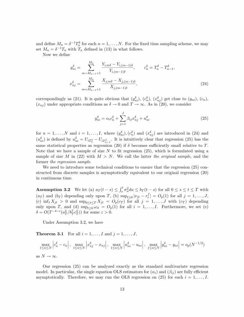
set Mn = δ−1Tn with Tn defined in (13) in what follows.Now we define

yδni =

Mn∑

m=Mn−1+1

Yi,mδ − Yi,(m−1)δ

Yi,(m−1)δ, cδ

n = T δn − T δ

n−1,

xδnj =

Mn∑

m=Mn−1+1

Xj,mδ −Xj,(m−1)δ

Xj,(m−1)δ, (24)

correspondingly as (21). It is quite obvious that (yδni), (cδ

n), (xδnj) get close to (yni), (cn),

(xnj) under appropriate conditions as δ → 0 and T →∞. As in (20), we consider

yδni = αic

δn +

J∑

j=1

βijxδnj + uδ

ni (25)

for n = 1, . . . , N and i = 1, . . . , I, where (yδni), (c

δn) and (xδ

nj) are introduced in (24) and(uδ

ni) is defined by uδni = UiT δ

n− UiT δ

n−1. It is intuitively clear that regression (25) has the

same statistical properties as regression (20) if δ becomes sufficiently small relative to T .Note that we have a sample of size N to fit regression (25), which is formulated using asample of size M in (22) with M > N . We call the latter the original sample, and theformer the regression sample.

We need to introduce some technical conditions to ensure that the regression (25) con-structed from discrete samples is asymptotically equivalent to our original regression (20)in continuous time.

Assumption 3.2 We let (a) aT (t − s) ≤ ∫ ts σ2

udu ≤ bT (t − s) for all 0 ≤ s ≤ t ≤ T with(aT ) and (bT ) depending only upon T , (b) supt≥0 |νjt − rf

t | = Op(1) for all j = 1, . . . , J ,(c) inft Xjt > 0 and sup0≤t≤T Xjt = Op(cT ) for all j = 1, . . . , J with (cT ) dependingonly upon T , and (d) supt≥0 ωit = Op(1) for all i = 1, . . . , I. Furthermore, we set (e)δ = O(T−4−ε(a2

T /b7T c4

T )) for some ε > 0.

Under Assumption 3.2, we have

Theorem 3.1 For all i = 1, . . . , I and j = 1, . . . , J ,

max1≤n≤N

∣∣∣cδn − cn

∣∣∣ , max1≤n≤N

∣∣∣xδnj − xnj

∣∣∣ , max1≤n≤N

∣∣∣uδni − uni

∣∣∣ , max1≤n≤N

∣∣∣yδni − yni

∣∣∣ = op(N−1/2)

as N →∞.

Our regression (25) can be analyzed exactly as the standard multivariate regressionmodel. In particular, the single equation OLS estimators for (αi) and (βij) are fully efficientasymptotically. Therefore, we may run the OLS regression on (25) for each i = 1, . . . , I.

13

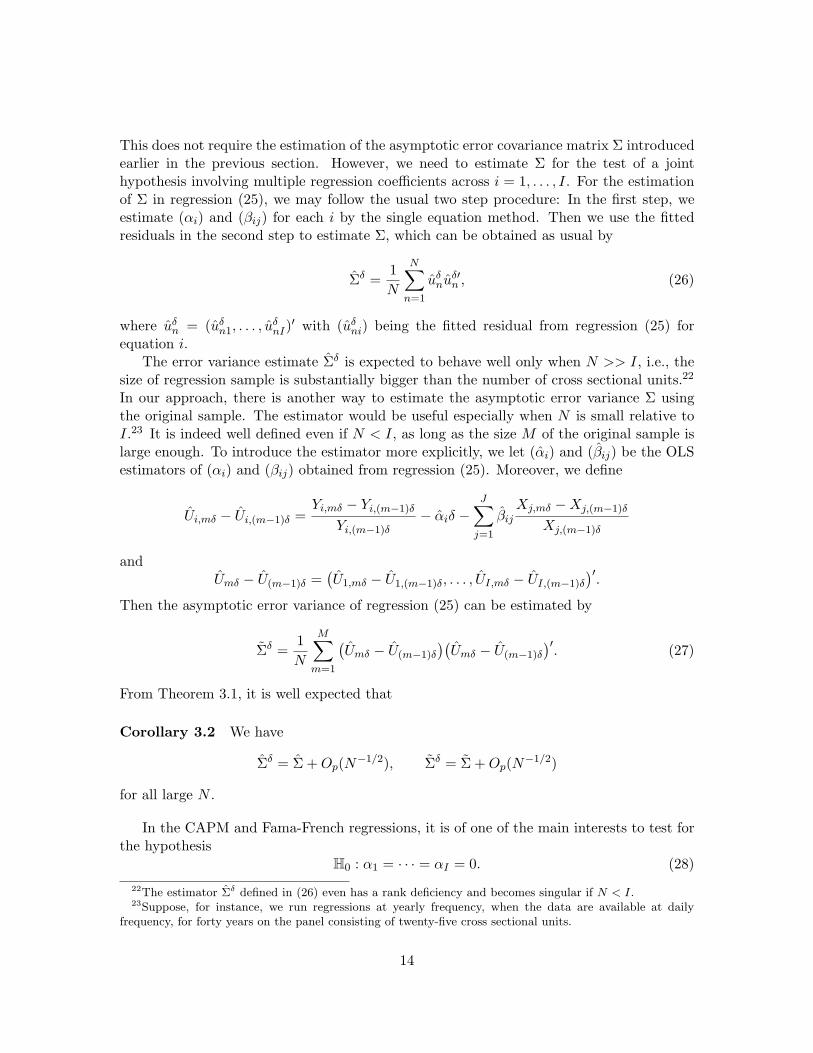
This does not require the estimation of the asymptotic error covariance matrix Σ introducedearlier in the previous section. However, we need to estimate Σ for the test of a jointhypothesis involving multiple regression coefficients across i = 1, . . . , I. For the estimationof Σ in regression (25), we may follow the usual two step procedure: In the first step, weestimate (αi) and (βij) for each i by the single equation method. Then we use the fittedresiduals in the second step to estimate Σ, which can be obtained as usual by

Σδ =1N

N∑

n=1

uδnuδ′

n , (26)

where uδn = (uδ

n1, . . . , uδnI)

′ with (uδni) being the fitted residual from regression (25) for

equation i.The error variance estimate Σδ is expected to behave well only when N >> I, i.e., the

size of regression sample is substantially bigger than the number of cross sectional units.22

In our approach, there is another way to estimate the asymptotic error variance Σ usingthe original sample. The estimator would be useful especially when N is small relative toI.23 It is indeed well defined even if N < I, as long as the size M of the original sample islarge enough. To introduce the estimator more explicitly, we let (αi) and (βij) be the OLSestimators of (αi) and (βij) obtained from regression (25). Moreover, we define

Ui,mδ − Ui,(m−1)δ =Yi,mδ − Yi,(m−1)δ

Yi,(m−1)δ− αiδ −

J∑

j=1

βij

Xj,mδ −Xj,(m−1)δ

Xj,(m−1)δ

andUmδ − U(m−1)δ =

(U1,mδ − U1,(m−1)δ, . . . , UI,mδ − UI,(m−1)δ

)′.

Then the asymptotic error variance of regression (25) can be estimated by

Σδ =1N

M∑

m=1

(Umδ − U(m−1)δ

)(Umδ − U(m−1)δ

)′. (27)

From Theorem 3.1, it is well expected that

Corollary 3.2 We have

Σδ = Σ + Op(N−1/2), Σδ = Σ + Op(N−1/2)

for all large N .

In the CAPM and Fama-French regressions, it is of one of the main interests to test forthe hypothesis

H0 : α1 = · · · = αI = 0. (28)

22The estimator Σδ defined in (26) even has a rank deficiency and becomes singular if N < I.23Suppose, for instance, we run regressions at yearly frequency, when the data are available at daily

frequency, for forty years on the panel consisting of twenty-five cross sectional units.

14

The rejection of the hypothesis implies that the proposed model is not a true model andpresumably requires a new factor.

The Wald test for the hypothesis can be easily formulated in our model (25), which maysimply be regarded as the classical multivariate regression. The test statistic τ(α) is definedby

τ(α) =(c′c− c′X(X ′X)−1X ′c

)−1α′Σ−1α, (29)

where c is an N -dimensional vector with cδn as its n-th component and X is an N × J

matrix with xδnj as its (n, j)-th element, and Σ = Σ or Σ. The test statistic τ(α) has

chi-square limit distribution with I-degrees of freedom. As discussed, we need some extratechnical conditions if we use Σ. It is also possible to use F -distribution after an appropriateadjustment for the degrees of freedom, as in Gibbons, Ross and Shanken (1989).24 We maysimilarly test the hypothesis H0 : β1j = · · · = βIj = 0 for some factor j, using the statistic

τ(βj) =(x′jxj − x′jX

cj (X

c′j Xc

j )−1Xc′

j xj

)β′jΣ

−1βj (30)

where xj is an N -dimensional vector with xδnj as its n-th component and Xc

j is an N × Jmatrix defined by deleting the j-th column from X and adding c as one of its columns.

In order are some discussions on how we deal with the presence of jumps. Our theoreticaldevelopment thus far assumes that the error process is given by a process with a continuoussample path a.s. However, for the validity of our econometric methodology, we do not needto assume that the error process is continuous. Indeed, our random sampling scheme iswell expected to remove endogenous and nonstationary volatilities even in the presence ofjumps. In this case, the DDS theorem does not apply and the regression errors are notin general normally distributed. Nevertheless, this does not affect our statistical theory,since it does not rely on the normality of the regression errors. In fact, following Choi andPark (2010), it is rather straightforward to show that Assumption 2.1 continues to hold ingeneral if the error processes (Ui) are discontinuous and have jumps, with Σ given by theprobability limit of Σ and Σ introduced respectively in (17) and (19). A variety of jumpsmay be allowed as long as they occur exogenously in discrete time intervals. Moreover, wecan show as in Choi and Park (2010) that the presence of jumps in (Ui) does not affect theasymptotic validity of all our subsequent procedures to analyze continuous time processesusing discrete observations.

To be more consistent with our theoretical model, however, we assume that jumpsare generated independently from the continuous part of the model and do not includeany information on the model parameters. Therefore, jumps are regarded as pure noise.Accordingly, we simply get rid of the observations that appear to be contaminated withjumps for our empirical analysis in the paper. We first use a test by Lee and Mykland(2008) to find the locations of jumps. Once we find their locations, we identify the samplingintervals [T δ

n−1, Tδn ] to which they belong, and simply discard the corresponding regression

24Strictly speaking, their test, often referred to as the GRS test in the literature, is not applicable in ourcontext, since we do not assume normality. Of course, the estimation samples would be closer to normalunder the random sampling scheme, and it would be more appropriate to use the random sampling schemefor the GRS test. We do not report their test in the paper, however, since in our case the degrees of freedomadjustment is negligible and their tests always yield the same results qualitatively as the Wald tests.

15

samples.25 It is also possible that we test for the presence of jumps in each of the timeintervals [T δ

n−1, Tδn ], n = 1, . . . , N , using the test developed by, e.g., Barndorff-Nielson and

Shepard (2004b), and delete the regression samples from any of the time intervals which aretested positive. This procedure, however, makes sense only when sufficiently large enoughnumber of the original samples exist in all of the time intervals.

There are various methods developed in the literature that are comparable to our pro-cedure in the paper. Andersen, Bollerslev, Diebold and Wu (2006), Barndorff-Nielsen andShephard (2004a) and Todorov and Bollerslev (2007) all consider the inferential problemin continuous time regression model similar to ours. Indeed, we may directly apply theirmethods to estimate (βi) in our regression model (6).26 However, their approach is differentfrom ours in that they fix T and let δ → 0. They focus more on the analysis of quadraticcovariations of the regressands and regressors in continuous time over a fixed time interval.It would therefore be more appropriate to apply their methods for ultra-high frequencysamples observed over a relatively short time horizon. In contrast, our methodology wouldbe more useful to analyze continuous time regression model over longer time horizons, sincewe require T → ∞ as well as δ → 0. For the inference on constant term (αi) in regression(6), none of the aforementioned existing methods is applicable and it is absolutely necessaryto utilize samples over long time horizons. In particular, all other existing methods are notapplicable to test for the hypothesis (28).

The original Fama-French regressions and their variants have largely been analyzed indiscrete time models using low-frequency observations spanning relatively long time hori-zons. It is possible to accommodate the presence of nonstationary stochastic volatilities indiscrete time framework. In fact, various discrete-time regression models with nonstation-ary stochastic volatilities are suggested and studied by several authors including Hansen(1995), Chung and Park (2007) and Xu (2007). In particular, we may apply the methodolo-gies developed in Hansen (1995) and Chung and Park (2007) to do inference in appropriatediscrete-time models corresponding to our continuous-time model (6). However, the form ofnonstationary stochastic volatility we may consider in discrete-time model is rather limitedand somewhat unrealistic. The required statistical procedure to properly deal with the pres-ence of nonstationary stochastic volatility is nevertheless quite complicated and difficult toimplement. On the other hand, our continuous time approach permits truly general nonsta-tionary stochastic volatility, and provides a very simple yet extremely powerful methodologyto effectively deal with it.

25Of course, this pretesting on jumps would render the size of the subsequent test deviate from its nominaltest. This is, however, ignored for simplicity.

26As shown in Barndorff-Nielsen and Shephard (2004a), (βi) in (6) can be estimated consistently simply bythe usual high-frequency regression without constant term, if δ → 0 with T fixed. It can be shown that theregression continues to yield a consistent estimate for (βi) under our setup requiring T →∞. The inclusionof constant term (αi) does not affect the consistency of the estimate for (βi), as long as the integrated

regressors (∫ T

0dXjt/Xjt) are not exceedingly explosive.

16

4. Data and Preliminary Analysis

4.1 Data

This section describes the data sets used in our empirical analysis. We make use of decileportfolios stratified by sizes, book-to-market ratios (B/M), and past performances. We alsouse 25 portfolios sorted by sizes and B/M and 30 industry portfolios. All the data setsare available at Kenneth French’s web page.27 For pricing factors, we adopt the market(MKT ), the size (SMB), and the B/M (HML), often referred to as the Fama-Frenchfactors, and the momentum factor (MMT ). The data sets cover the period of July, 1963and December, 2008, and all of the returns in the data sets are of the daily frequencyand annualized. Table 1 presents summary statistics of the factors and the correspondingportfolio returns. Specifically, Panel A reports means and standard deviations of the factors,together with correlations across each other. High Sharpe ratios of HML and MMTstate that buying and holding distressed firms or better performing firms would have beenlucrative investment strategies during this period. In terms of correlations, both SMB andHML have moderately negative correlations with MKT , while MMT is weakly, negativelycorrelated with MKT . Correlations across SMB, HML, and MMT are small. Panel Bof Table 1 reports means and standard deviations of annualized returns stratified into tenportfolios. The eleventh row in each group refers to portfolio strategies with long positions ofhigh returns and short positions of low returns, often called the hedged portfolio returns.28

The size strategy yields about 1.6% per annum, while the book-to-market strategy earnsabout 5.6% per annum. During this period, the momentum strategy of buying past winnersand selling past losers produces 18% per year, which is quite substantial. These summarystatistics suggest that they are good candidates for pricing factors, as discussed in theprevious literature. How about the volatility structures of these portfolio returns? Wedelve into this issue in the next subsection.

4.2 Preliminary Analysis

Our factor pricing model specified in (6) and (7) imposes some special error structure inthe Fama-French regressions, which motivated us to invent a new methodology. Before wereexamine the Fama-French regressions using our methodology, it is therefore necessary thatwe investigate whether various specifications of our model are empirically justifiable. Forthis purpose, we consider the conventional 3-factor Fama-French regression which uses 25portfolio returns sorted by size and book-to-market ratio as regressands and Fama-Frenchfactors as regressors.

An important implication of the Assumption 2.1 is that the error processes (dUi) in (6)are correlated cross-sectionally due to the presence of the common component (dWk).29 To

27http://mba.tuck.darthmouth.edu/pages/faculty/ken.french/index.html28This, respectively, corresponds to (i) the returns from the smallest size (1st group) of market equity

minus the returns from the largest size (10th group) for the size strategy, (ii) the returns from the highestB/M (10th group) minus the lowest B/M (1st group) for the book-to-market strategy, and (iii) the returnsfrom the winner (10th group) minus the loser (1st group) in case of the momentum strategy.

29Independence of (ωi, Zi) and (ωi) is not likely to be empirically testable by construction. However,

17

see how much cross-correlations exist among the errors in a typical factor pricing model,we test for diagonality of the covariance matrix of fitted residuals estimated in the usualway from the aforementioned conventional Fama-French regression. We use the residualsfrom both fixed time regression and our new random time regression, which was formallyintroduced in (25), and apply the LM test of diagonality suggested by Breusch and Pagan(1980). As can be seen in Table 2, the null of diagonality is rejected in both cases, indicatingthat there exist cross-correlations among the errors, which may be generated by the commonerror component (dWk) or a common error component not captured by the factors alreadyincluded.

Our specification of the pricing formula given in (6) and (7) presumes the presenceof common volatility factor σ in the diffusion terms (dVj) of all pricing factors (dQj/Qj)specified in (3) and more importantly in the common component (dWk) of the errors (dUi).Especially, we assume that the common volatility factor σ is given by the volatility of theexcess market return which is defined from the first pricing factor as in (11). To see if thisassumption is empirically justified, we plot the quadratic variation series of daily excessmarket return along with those of the daily 25 fitted residuals from the Fama-French threefactor regression in Figure 1.30 It is clear that the 25 residual quadratic variation seriesfollow closely that of the excess market return signified by the dark thicker line, therebystrongly supporting our assumption that the volatility of excess market return representsthe common component of individual residual volatilities.

To more carefully investigate the appropriateness of our assumption, we also estimatethe instantaneous variances of the 25 fitted residuals and compare them with those of theexcess market returns. Note that the quadratic variation series presented in Figure 1 canbe regarded as the estimates for the integrated variances of the fitted residuals, and thatthe instantaneous variances are the time derivatives of integrated variances. For the actualestimation, we apply the local linear smoothing method to the quadratic variation serieswe obtained earlier and compute their time derivatives. We also conduct the principalcomponent analysis to extract the leading factor from the estimates of the instantaneousvariances for the fitted residuals. The leading factor is expected to represent the nonsta-tionary volatility factor in the fitted residuals. Our results are provided in Figure 2. Themagnitudes of the estimated instantaneous variances of the fitted residuals are not exactlyidentical to those of the market, or those of the extracted leading factor. However, it israther strongly suggested that they fluctuate together. In particular, their cycles are re-markably overlapped. For instance, the timings of peaks and troughs for the instantaneousvariance series of the market and the extracted leading factor appear to coincide perfectly.

We also investigate whether the errors (uni) are orthogonal to the regressors (cn) and(xnj) in our regression (20), especially under random sampling scheme. Of course, this iscrucial for the validity of OLS procedure. Indeed, they may be correlated with each other.It happens, for instance, if the pricing factors (dQj/Qj) in (3) has nonpricing volatilitycomponents (dWk), as well as the pricing volatility components (dVj). To see whether the

whether there is a common component in error terms is a fair empirical question, which we illustrate inshort.

30To obtain the residuals at the daily level, we use the coefficient estimates from the random time Fama-French three factor regression.

18

orthogonality between the regressors and the regression errors is a plausible tenet, we runthe fixed time regression using monthly observations to estimate the regression coefficients,and use the estimates to obtain the fitted residuals at the daily frequency. Then we obtainthe time change and compute the sample correlations between the regressors (cn) and (xnj),and the regression errors (uni), for the random time regression. If the assumed orthogonalitydoes not hold, then we must have at least some evidence of nonzero correlation betweenthe regressors and the regression errors under the random sampling scheme. The resultsare reported in Table 3. The values of the actual sample correlations are quite low for allregressors, supporting the validity of OLS in the random time regressions.

Lastly, based on all the results, we are ready to check if the volatility structure we imposeon error terms is plausible and well treated by the random sampling scheme proposed inthe paper. To empirically evaluate this issue, we consider a stochastic volatility model tomeasure the degree of persistency in the stochastic volatilities of regression errors in (20).Therefore, we specify uni =

√fi(vni)εni for n = 1, . . . , N and i = 1, . . . , I with Eε2

ni = 1,where (vni) is the latent volatility factor generated as vni = ρivn−1,i + ηni and (fi) is thevolatility function. We use the logistic function for the volatility function fi, and allowfor nonzero correlation between (εni) and (ηni) which represents the leverage effect.31 Thestochastic volatility model is fitted for each i using the fitted residuals from regression (25)based on the random sampling scheme, and the latent volatility factor is extracted usingthe conventional density-based Kalman filter method. For comparison, we also estimate thestochastic volatility model using the fitted residuals from the fixed time regression. Theextracted volatility factors are given in Figures 3-5 and the estimated values of the ARcoefficients (ρi) of the extracted volatility factors are presented in Table 4.

It seems evident that the extracted volatility factors of the residuals from random timeregressions are not persistent. Note that the volatilities of the individual portfolios consistof both the nonstationary common trend and stationary idiosyncratic components, and onlythe nonstationary common component is corrected via our random sampling method. Thus,one may expect that the estimated AR coefficients in this case reflect only the stationarycomponent of the extracted volatilities. Indeed, the average of the estimated AR coefficientsis around 0.724 in the random time, which is stationary. This is in sharp contrast with thevolatility factors extracted from the fixed time residuals, most of which have the estimatedAR coefficient very close to unity. In addition, the observed high persistency of the volatilityfactors extracted from the fixed time residuals is quite similar to that of the fixed time excessmarket return, as can be seen in the first panel of Figure 6. The estimated AR coefficient ofthe fixed time market volatility factor is 0.9505.32 On the other hand, the AR coefficient ofthe extracted volatility factor from the time changed market return is much smaller, indeedclose to zero, and its sample path clearly shows no persistency as displayed in the secondpanel of Figure 6. Putting things together, the empirical results confirm that our volatilitysetup is realistic and properly handled with the random sampling scheme.

31The reader is referred to Kim, Lee and Park (2009) for more details about the stochastic volatility modeland estimation methodology we use in the paper.

32This is also consistent with the well known fact that the stochastic volatility of market return is highlypersistent. See aforementioned references for the nonstationarity in stock return volatilities.

19

5. Reexamination of Fama-French Regressions

5.1 Tests of the CAPM

In this section, we examine the CAPM regressions on five sets of daily portfolio returns. Firstthree sets consist of eleven portfolios, ten of which are sorted out by a firm characteristic(sizes, B/M ratios or prior returns), and the eleventh one refers to the hedge portfolioexplained in the previous section. The next set consists of thirty industry portfolios. Finally,the last data set comprises traditional 25 portfolios sorted by sizes and B/M ratios. Asdiscussed in Section 2, we run regression (9) under the two sampling schemes, fixed time andrandom time. In case of the fixed time sampling, we construct monthly data by integratingportfolio returns over each month. For the random time sampling scheme, we follow (12)and set ∆ at the level of quadratic variation comparable to the average, monthly excessmarket return. Tables 5 to 9 report estimates of alphas and betas with standard errors foreach portfolio, followed by the Wald statistic defined in (29) to test if the model is rejected.

Table 5 reports results for the decile size portfolios, and the size strategy (1st−10thdecile) portfolio. Beta estimates in both sampling schemes are close to each other andMKT mildly captures exposures to taking risks for small firms (i.e., beta is higher for smallfirms). However, comparing the alpha estimates, one can clearly see that there is a hugedifference between the fixed time and the random time sampling schemes. There existsa significant risk component not captured by the market factor according to small firms’alpha estimates in the random sampling case, whereas the fixed sampling result is muchweaker. As expected, the Wald test statistic states that the CAPM is not rejected in case ofthe fixed sampling regression, while p-value of the random sampling case is 0.0000, a clearrejection. Figure 7 displays this finding graphically. Fixed sampling results show a hump-shape of alpha estimates, which is somewhat confusing, if the size effect does matter. Onthe contrary, the random-sampling result with a proper treatment of stochastic volatilities,shows a nice emergence of monotonically decreasing size premium.

Table 6 reports basically the identical information for the book-to-market portfolios.However, this case shows another evidence that the conventional method fails in doingreliable statistical inferences. Unlike Table 5 with size-based portfolios, Table 6 reportthat both alphas and betas are similarly estimated, and the estimated amount of valuepremium is around 6% to 7% per annum. Figure 8 illustrates that the estimated alphas aresimilar across the two methods. However, when the Wald statistics are compared, the fixedsampling scheme cannot reject the CAPM, while the random sampling rejects the modelwith p-value of 0.0000. In addition, the estimated market betas dictate that the growthstocks are riskier than the value stocks, implying that the CAPM is probably not pricingthese portfolios correctly, as shown by Fama and French (1993).

Based on the results, we suspect that the model is correctly rejected in the random timeregressions, and the conventional fixed time regressions seem to have difficulty in doingthis. However, at this stage, a natural question arises: Fama and French (1993) and manyauthors have used the conventional OLS with the Gibbons, Ross, and Shanken (GRS) teststo reject the CAPM and even various other Fama-French models. Why do our fixed timesampling results differ from the previous OLS results? Recall that the main difference

20

between the conventional OLS and our fixed sampling OLS is the way that data series areconstructed. The conventional monthly return data use two data points of asset pricesbetween two consecutive months, while our data are constructed by integrating the dailydata over a month in fixed sampling cases. The two methods would produce the samemonthly data if the instantaneous returns were defined as the differentials of logarithm ofprices, viz., d log(Pi,t). However, our instantaneous returns are constructed as the ratios ofthe price differentials to previous prices, viz. dPi,t/Pi,t−1, and under this definition the twodata construction methods can produce substantially different monthly return data.

But, can we, then, achieve the same results by directly using the monthly return datawith the conventional OLS machinery instead of using random sampling scheme on a higherfrequency data, because both will take a look at the data at a frequency comparable tomonthly frequency after all? Note that our model is written in continuous time, thenaggregated over time to make the model testable in discrete time environment. As shownin Section 3, the asymptotics and resultant test statistics of the model are different fromthose of the discrete-time counterparts. If continuous time diffusion models better describethe actual market clearing processes, which we believe, then, these differences are critical inevaluating the empirical asset pricing models. To further investigate this point, we run theOLS regressions on the conventional monthly returns with the same decile portfolios. Wefind two interesting results. First, in both size and B/M based decile portfolios, the GRSstatistics report p-values around 0.031 and 0.038 respectively. Therefore, the CAPM is notrejected at 3% despite the prevalent size or value effects. Second, as we vary the startingdate of the data, p-values vary significantly between 0.002 and 0.208.33 This result may bean indirect evidence of conditional factor models. But, even in conditional models, a finaltest on whether a model is rejected would be to look at whether or not the long-run averageof alphas be zero.34 Thus, the use of low frequency data does not necessarily give reliableand accurate test results. On the contrary, our random sampling results are quite robust tosuch variations. This is a subtle but an important point: Conventional methods may failto reject a model too easily, and often produce puzzling results.

Table 7 and Figure 9 report the results on the momentum portfolios. The momentumstrategy generates a huge average abnormal returns of 20% to 22% in both cases and theCAPM is decisively rejected in both sampling regressions. Thus, putting things together,unless deviations from the true model are really obvious, like in the case with the momentumfactor, the conventional testing procedure is inoperable and fails to reject a proposed modeltoo often. As emphasized in our earlier discussions, the failure of the conventional testingprocedure is due to the fact that variance-covariance matrix of the error terms is verydifficult to estimate in the presence of non-stationary stochastic volatilities. Indeed, existingempirical studies unequivocally show that they are nonstationary, though their sources may

33Although not monotonic, CAPM on size portfolios is more difficult to reject when the sample period getslonger, while the opposite is likely to be true for the CAPM regressions on value portfolios. We do not reportthe results as a separate table since similar exercises have been performed in other studies. Nevertheless,our argument here is germane and new in the context of testing factor pricing models with nonstationaryvolatilities in a high frequency setting.

34See Ang and Kristensen (2009) for more details. They test conditional factor pricing models using anon-parametric method.

21

differ. And the models with time-varying and stochastic volatilities would yield misleadingresults, as we discussed earlier. In addition, the presence of leverage effects, also prevalentin stock return data, brings about endogeneity in volatilities, which further complicatesthe treatment of the nonstationary volatilities. We also run a similar exercise for the 25Fama-French portfolios sorted by sizes and B/M ratios and report the results in Table 8 andFigure 10. Now, even the fixed sampling scheme rejects the CAPM with p-value of 0.0000,which contradicts the test results with the decile portfolios. On the contrary, the randomsampling method rejects the model, compatible with the results from the decile portfolios.

As a final exercise for the CAPM, we examine the unmanaged industry portfolios con-sisting of thirty groups and report the results in Table 9. The familiar story prevails again.Despite the similar estimates of alphas and betas on average, Wald test statistics say thatthe conventional approach cannot reject the CAPM at 4.53%, while our approach rejectsthe model with zero p-value. To analyze what makes the difference between the two ap-proaches in this case, we plot the alphas connecting each industry that belongs to one ofmore broadly defined five groups of industries in Figure 11. Most conspicuous are the in-dustries in consumer goods group featuring consistently positive alphas in our random timeregression, while the fixed time regression produces a mixed bag of results. This suggeststhat consumption growth may be a valid pricing factor together with the financial marketfactor, which is reminiscent of consumption-based pricing models employing more flexiblepreferences such as Epstein and Zin (1989). Summing up, the random sampling methodworks reliably in a high-frequency environment, contrary to its fixed sampling counterpart.More importantly, all the test results for the CAPM based on the random sampling providea strong case for multi-factor models.

5.2 Tests of the Fama-French Models

In this section, we investigate multi-factor models of asset returns. Continued from the pre-vious section, we begin with two-factor models, incorporating the size, B/M or momentumfactor into the CAPM on each of the corresponding decile portfolio data sets. In Tables 10and 11, like the CAPM, the fixed time OLS regressions cannot reject the two-factor modelswith the factors (MKT ,SMB) and (MKT ,HML) at even higher p-values, stating that thesize and B/M factors are relevant pricing factors, despite that the CAPM is not rejectedon the same data sets. This is a contradicting result caused by the imprecise statisticalmethod. Meanwhile, the random sampling result shows that the two-factor model with theB/M is not rejected at 8% of p-value for the 10 B/M-based portfolios, though the model withthe size factor fails to explain the 10 size-based portfolios. That is, our method suggeststhat the B/M factor is indeed a valid pricing factor for explaining the variations of stockreturns over the cross-section of B/M ratio groups, while the size factor may be insufficientto account for the spectrum of asset returns in light of the firm sizes. In addition, we wantto note that this is consistent and plausible with the random-sampling CAPM results onsize groups that are decisive rejections. Table 12 reports that the two-factor model withthe momentum is rejected in both approaches.

One common feature in all three of the two factor models we consider here is that theabnormal returns of the hedged portfolios are not statistically different from zero, suggesting

22

that pricing errors are small. What then drives the rejections of the model according to theWald statistics in the random sampling case? A closer look at the Tables 10 and 12 revealsthat other portfolios than those used in forming the hedged portfolios, such as Size 5 orMomentum 3, turn out to have significantly non-zero abnormal returns. Thus, the Waldtest for all assets, compared to the test on a hedged portfolio alone, is a more stringenttest for verifying if a factor model can explain all the returns considered than just the onesspecifically aimed at matching certain characteristics. Therefore, if the results between thetwo tests in a factor pricing model clearly disagree, then the proposed model may neednew factors because it is likely to have difficulty in fitting the returns sorted by othercharacteristics. Consistent with this view, Table 11 shows that the medium value stocks aswell as the hedged portfolio do not have significantly non-zero abnormal returns, hence themodel is not rejected.

Based on this observation and following the tradition, now we estimate and test thethree-factor Fama-French model on the data set with 25 portfolios. Tables 13 and 14 showthat both fixed and random time regressions reject the model. This result is somewhatanticipated from the random sampling results on the two factor model (MKT, SMB) inTable 10, where the size factor fails to explain the 10 size-based portfolios. Compared tothe CAPM results on the 25 portfolios, the extent to which the model misbehaves appearsto be smaller, yet the p-values based on Wald statistic imply a clear rejection of the Fama-French model, which requires careful scrutiny. The first panels for the fixed and randomtime regressions in Figure 12 display the deviations of alpha estimates from zero for the25 portfolios. The first group consisting of the smallest stocks have the largest magnitudeof deviations, which is a common feature in both the fixed sampling and random samplingcases. Related, the two graphs in second panels of Figure 12 connect the alpha estimateswith either the same sizes or B/M groups. Compared to the corresponding graphs in Figure10 for the CAPM, the lines are much closer to the horizontal axis of zero value and even theslope is obviously reversed in some cases. However, one observation, corresponding to (size,B/M) = (1, 1) distinctively deviates from zero value, which seems to drive the rejection ofthe model. Note that this refers to small cap, growth stocks with low book-to-market ratios.To be more precise, we plot the average excess returns for each portfolio and the predictedreturns from the Fama-French regressions in Figure 13, following Cochrane (2001, p441).It is easy to observe that the (1, 1) portfolio is quite off from the 45 degree line comparedto other portfolios and it displays a significant premium within the smallest B/M group.35

This is a part of the size premium, yet we must note that the lower, left panels in Figures 12and 13 display that the small growth stocks show the stark contrast to the typical pattern ofthe size premium, hinting that the conventional size factor may be not enough in capturingthis behavior.36 This suggests that either an additional factor or a replacing factor may be

35This effect also appears in Cochrane (2001) yet with a much weaker pattern. We suspect that thedifference comes from the data period which is between 1947 to 1996 in his case.

36There may be a common economic fundamental that affects both size and B/M portfolio returns in adifferent fashion than the conventional size and B/M factors do. Fama and French (1995) report that boththe size and B/M premiums are related to the earnings of the firms. They find that the small firms havepersistently lower earnings and the growth stocks have persistently high earnings, though the former linkis weak. If persistent high earnings imply low cash flow risk, and the small firm effect is dominated by the

23

needed to justify premiums related to buying large cap stocks and selling small cap stocksin the group of firms with small distress.37

We recall that the portfolio returns from the consumer goods industry feature significantabnormal returns when CAPM is used. Admittedly, there is no direct connection betweenthe small growth stocks and the consumer goods industry. However, given the signifyingrole of consumption goods as a foundational link between a discount factor and asset prices,we believe that including the consumption sector returns as a factor is a worthy trial.Related, Lettau and Ludvigson (2001) found that a macroeconomic factor that captures theconsumption wealth ratio can substantially improve the performance of the consumptionCAPM. Motivated by those findings, we form a consumer goods industry factor, called theCMR factor as the excess returns on the portfolio of the firms producing consumer goods.Regarding the definition of the consumer goods sector, we simply use the returns from theconsumer goods sector out of the data with 5-industry category available in the KennethFrench’s data library. Then, we run regressions of multi-factor models incorporating theconsumer goods industry factor (CMR) on the 10 size-based and B/M-based portfolios, andthe 25 portfolios to see if a model with the CMR factor can help explain the behaviors ofasset returns, especially the small growth stocks. We report the results from three-factormodels, which include the market, the CMR and either the size or B/M factor.38

Table 15 displays the results from the three-factor models with the CMR factor on theportfolios sorted by the size and B/M ratio.39 In comparison with the results in Tables10 and 11, we observe that p-values increase in each case and the beta coefficients for theCMR are mostly significant. Thus, it is inferred that the CMR factor helps explain boththe value-based and size-based portfolios. Especially, the model with the market, B/M andCMR factors is not rejected at 10%.40 Figure 14 shows that the overall fit is good for bothof the three-factor models. Based on this positive result, we select these two three-factormodels to investigate the 25 portfolios. Unfortunately, both models are rejected at 0.0000of p-values, but we find that in case of the model with the market, B/M and CMR factors,the pricing error for the (1,1) portfolio gets significantly reduced and the overall fit appearsto be generally comparable to that of the Fama-French model. This is summarized in Table16 and Figure 15. For the model with the market, size and CMR, overall fit is worse andthe Wald statistic is higher, hence it is clearly inferior to the model with the market, B/Mand CMR, as well as the traditional Fama-French model. The results suggest that the sizefactor is not entirely satisfactory in terms of capturing the cross sectional behaviors of asset

value effect, this story may justify why a small, growth stock is a good asset to short-sell. However, it stilldoes not explain why the large cap within the smallest B/M ratio is a risky bet as illustrated in the lowerleft panel of the Figure 12.

37As one of the usual suspects, we try the momentum factor, making a four-factor model. However, wefind that the momentum factor is orthogonal to the size effect within low book-to-market ratios.

38We also tried the two-factor model consisting only of the market and the CMR. To conserve the spacewe do not report the results here but it appears that the CMR factor captures some of the size premiums,but not the value premiums.

39From now on, we only report the random sampling results, because the fixed sampling results on theindustry portfolio do not pick up the CMR factor as shown in Table 9 and Figure 11.

40When we estimated a four-factor model, i.e., the Fama-French 3-factor model with the CMR factor, wefind that the p-values get lower to 0.0000 and 0.0003 for the B/M and size portfolios, respectively.

24

returns and the returns from the consumer goods industry are useful in complementingthis deficiency. However, further investigation is necessary to incorporate both the size andconsumer factors into the factor pricing model since the four factor model has a much lowerp-value in spite of the additional factor.

6. Conclusion

This paper develops a new econometric framework and tools to analyze multi-factor assetpricing models. We consider a continuous-time factor model with a specific error compo-nent structure consistent with an underlying asset pricing theory. We show that our errorstructure is empirically supported as well. It is well known that asset returns have highlypersistent, time-varying and stochastic volatilities which can substantially harm the relia-bility of estimation and testing of asset pricing models, especially when a higher samplingfrequency is chosen. We overcome this difficulty by using samples collected at random inter-vals, instead of those sampled at calendar time. Specifically, the clock is running inverselyproportional to the market volatility. That is, a time interval is short when volatilities arehigh, and vice versa. Under our random sampling scheme, Fama-French regressions maysimply be regarded as the classical regressions having normal errors with variance givenby the averaged quadratic variation of the martingale differential errors. Our method isquite simple: We run the usual OLS regressions on the time-changed data so that potentialcomplexities from handling high-frequency data and nonstationary volatilities do not arise.

We apply our methods to various portfolios sorted by certain characteristics used toidentify pricing factors. We find that the tests based on conventional regression modelson fixed time intervals often produce invalid and contradicting test results. These issuesdo not prevail in the random time regressions. Even in comparison with the conventionalregressions on lower frequency data, our test appear to yield more reliable results. Ouradditional empirical findings can be highlighted as follows. First, size premium is still animportant part of cross sectional return variations. According to the fixed sampling scheme,size strategy produces around 0.6% annually, while our random sampling regression statesaround 5.6% per annum. In addition, even after including the size factor, the size-basedportfolios are not fully explained. This is not the case for the value-based portfolios. Second,we also find that the three-factor or four-factor Fama-French models cannot fully accountfor the size, value, and momentum premia, and the rejection of the three-factor modelappears to mainly come from the small firms with low book-to-market ratios in case ofthe 25 portfolios sorted by the size and book-to-market ratios. Of course, this is welldocumented in Fama and French (1993). However, we want to point out that althoughFama and French argue that their model still explains cross sectional variations very welldespite this puzzling behavior, this effect does not only survive over time but appears to geteven stronger according to our empirical results. Third, our CAPM and multi-factor resultson industry portfolios suggest some potential role to be played by an additional factor basedon consumer goods industry sector. It is noteworthy that this anomaly does not prevail inthe fixed sampling case.

In an attempt to find out a better factor pricing model, we form a consumer factor using

25

the returns from the consumer goods industry sector and test the model on all the portfolioswe consider. Interestingly, we find that this consumer factor has some explanatory poweron the returns of the small growth stocks. This suggests that factors motivated by economictheories can shed light on the issue of explaining the cross sections of stock returns, becausethese factors are likely to be robust to alternative sets of portfolios to be explained. Related,a recent work by Fama and French (2008) shows that there are many other asset pricinganomalies related to net stock issues, accruals, asset growth, and profitability. Some of themare even robust across all size groups, and the conventional Fama-French model is not ableto deliver satisfying performance. In this vein, a quest for valid pricing factors thereby anew and better asset pricing model is still an important task to sharpen our understandingon how financial markets reward taking systematic risks and uncertainties. We hope thatour newly developed tool is a useful addition to this enterprise.

Mathematical Appendix

Useful Lemmas and Their Proofs

Let (At) be an Ito process given by

dAt

At= ftdt + gtdBt,

where (Bt) is a Brownian motion with respect to a filtration (Ft), to which (ft) and (gt)are adapted. We assume

Assumption A1 For all 0 ≤ s ≤ t ≤ T , aT (t − s) ≤ ∫ ts g2

udu ≤ bT (t − s), where aT andbT are some constants depending only upon T .

Assumption A2 supt≥0 |ft| = Op(1).

Assumption A3 inft≥0 At > 0 and sup0≤t≤T At = Op(cT ), with (cT ) depending only onT .

In the subsequent development of our theory, we assume that the Ito process A satisfiesAssumptions A1-A3.

Lemma A1 We have

sup|s−t|≤δ

|At −As| = Op

(δ1/2−εb

1/2T cT

)

for any ε > 0, uniformly in 0 ≤ s, t ≤ T .

26

Proof of Lemma A1 Write

At −As =∫ t

sfuAudu +

∫ t

sguAudBu

for 0 ≤ s ≤ t ≤ T . We may easily deduce that∣∣∣∣∫ t

sfuAudu

∣∣∣∣ ≤(

sup0≤t≤T

At

)∫ t

s|fu|du = Op(δcT ) (31)

uniformly in 0 ≤ s, t ≤ T , due to Assumptions A2 and A3. Moreover, if we let Ct =∫ t0 gsAsdBs, then C is a continuous martingale with

[C]t − [C]s =∫ t

sg2uA2

udu

≤(

sup0≤t≤T

A2t

)∫ t

sg2udu = Op(δbT c2

T ) (32)

uniformly in 0 ≤ s, t ≤ T . Since C is a continuous martingale, we may represent it as

Ct = (D ◦ [C])t (33)

with the DDS Brownian motion D of C, due to the celebrated theorem by Dambis, Dubinsand Schwarz in e.g., Revuz and Yor (1993, Theorem 5.1.6, p173). Now we may deduce from(33), together with the modulus of continuity of Brownian motion and (32), that

sup|t−s|≤δ

|Ct − Cs| ≤ sup|t−s|≤δ

∣∣(D ◦ [C])t − (D ◦ [C])s

∣∣

≤ sup|t−s|≤δ

∣∣[C]t − [C]s∣∣1/2−ε = Op

(δ1/2−εb

1/2T cT

)(34)

for any ε > 0, uniformly in 0 ≤ s, t ≤ T . Upon noticing that cT δ = o(δ1/2−εbT cT

)for

any ε > 0, the stated result follows immediately from (31) and (34). The proof is thereforecomplete. ¤

Lemma A2 We have

max1≤m≤M

∣∣∣∣∣∫ mδ

(m−1)δ

dAt

At− Amδ −A(m−1)δ

A(m−1)δ

∣∣∣∣∣ = Op(δ1−εbT cT )

for any ε > 0.

Proof of Lemma A2 Define

Rm =∫ mδ

(m−1)δ

dAt

At− Amδ −A(m−1)δ

A(m−1)δ

=∫ mδ

(m−1)δ

(1− At

A(m−1)δ

)dAt

At=

∫ mδ

(m−1)δ

At −A(m−1)δ

A(m−1)δ(ftdt + gtdBt) . (35)

27

We have∫ mδ

(m−1)δ

At −A(m−1)δ

A(m−1)δftdt ≤ 1

inft At

(sup

(m−1)δ≤t≤mδ|At −A(m−1)δ|

)∫ mδ

(m−1)δftdt

= Op

(δ3/2−εb

1/2T cT

)= Op

(δ1−εbT cT

)(36)

uniformly in m = 1, · · · ,M , due in particular to Lemma A1. Moreover,∫ t

(m−1)δ

As −A(m−1)δ

A(m−1)δgsdBs

is a continuous martingale, whose increment in quadratic variation over interval [(m −1)δ,mδ] is bounded by

∫ mδ

(m−1)δ

(At −A(m−1)δ

A(m−1)δ

)g2t dt ≤ 1

inft A2t

(sup

(m−1)δ≤t≤mδ|At −A(m−1)δ|2

)∫ mδ

(m−1)δg2t dt

= Op

(δ2−εb2

T c2T

).

Consequently, we may show that∫ mδ

(m−1)δ

At −A(m−1)δ

A(m−1)δgtdBt = Op

(δ1−εbT cT

)(37)

uniformly in m = 1, · · · , M , using the same argument as in the proof of Lemma A2. Thestated result now follows immediately from (35), (36) and (37). ¤

Subsequently, we let

dFt =dAt

Atand dGt = gtdBt,

and define

[F ]δt =∑

mδ≤t

(Amδ −A(m−1)δ

A(m−1)δ

)2

[G]δt =∑

mδ≤t

(Gmδ −G(m−1)δ)2.

Lemma A3 We have

sup0≤t≤T

∣∣∣[G]δt − [G]t∣∣∣ = Op

((δT )1/2bT

).

Proof of Lemma A3 Under Assumption A1, the stated result follows immediately fromLemma A3.1 of Park (2009).

28

Lemma A4 We have

sup0≤t≤T

∣∣∣[F ]δt − [G]t∣∣∣ = Op

(δ1/2−εTb

3/2T c2

T

)

for any ε > 0.

Proof of Lemma A4 Define

[F δ]t =∑

mδ≤t

(Fmδ − F(m−1)δ)2 =

∑

mδ≤t

(∫ mδ

(m−1)δ

dAt

At

)2

,

and note that ∣∣∣[F ]δt − [G]δt∣∣∣ ≤

∣∣∣[F ]δt − [F δ]t∣∣∣ +

∣∣∣[F δ]t − [G]δt∣∣∣ . (38)

We may readily deduce from Lemmas A1 and A2 that

∣∣∣[F ]δt − [F δ]t∣∣∣ =

∑

mδ≤t

(Amδ −A(m−1)δ

A(m−1)δ

)2

−(∫ mδ

(m−1)δ

dAt

At

)2

≤ 2inft At

(max

1≤m≤M|Amδ −A(m−1)δ|

)

M

(max

1≤m≤M

∣∣∣∣∣∫ mδ

(m−1)δ

dAt

At− Amδ −A(m−1)δ

A(m−1)δ

∣∣∣∣∣

)

=(T/δ)Op

(δ1/2−εb

1/2T cT

)Op

(δ1−εbT cT

)= Op

(δ1/2−εTb

3/2T c2

T

)(39)

for all 0 ≤ t ≤ T .Moreover, it follows that

[F δ]t = [G]δt + 2∑

mδ≤t

(∫ mδ

(m−1)δftdt

)(Gmδ −G(m−1)δ) +

∑

mδ≤t

(∫ mδ

(m−1)δftdt

)2

,

where we have∑

mδ≤t

(∫ mδ

(m−1)δftdt

)2

≤ MOp(δ2) = Op(δT )

and∣∣∣∣∣∣∑

mδ≤t

(∫ mδ

(m−1)δftdt

)(Gmδ −G(m−1)δ)

∣∣∣∣∣∣

≤ ∑

mδ≤t

(∫ mδ

(m−1)δftdt

)2

1/2 ∑

mδ≤t

(Gmδ −G(m−1)δ)

1/2

= Op

((δT )1/2

)Op

((TbT )1/2

)= Op

(δ1/2Tb

1/2T

)

29

uniformly in 0 ≤ t ≤ T . Note that δT = o(δ1/2Tb

1/2T

). Consequently, we have

∣∣∣[F δ]t − [G]δt∣∣∣ = Op

(δ1/2Tb

1/2T

)(40)

uniformly in 0 ≤ t ≤ T . The stated result follows from Lemma A3, and (38), (39) and (40).Note that

δ1/2Tb1/2T , (δT )1/2bT = o

(δ1/2−εTb

3/2T c2

T

),

and therefore, the terms we consider in Lemma A3 and (40) become negligible. ¤In what follows, we let

Ht = infs>0

{[G]s > t

}

and analogously defineHδ

t = infs>0

{[F ]δs > t

}

for 0 ≤ t ≤ [G]T .

Lemma A5 We have

sup0≤t≤[G]T

∣∣∣Hδt −Ht

∣∣∣ = Op

(δ1/2−εTa−1

T b3/2T c2

T

)

for any ε > 0.

Proof of Lemma A5 The proof is virtually identical to that of Corollary 3.3 of Park(2009), and therefore, it is omitted.

In the following lemma, we define Mn by δMn = Hδn∆ for n = 1, . . . N .

Lemma A6 We have

max1≤n≤N

∣∣∣∣∣∣

∫ Hn∆

H(n−1)∆

dAt

At−

Mn∑

m=Mn−1+1

Amδ −A(m−1)δ

A(m−1)δ

∣∣∣∣∣∣= Op

(δ1/4−εT 1/2a

−1/2T b

5/4T cT

)

for any ε > 0.

Proof of Lemma A6 We let

Rn =∫ Hn∆

H(n−1)∆

dAt

At−

Mn∑

m=Mn−1+1

Amδ −A(m−1)δ

A(m−1)δ,

and write|Rn| ≤ |Ra

n|+∣∣∣Rb

n

∣∣∣ , (41)

30

where

Ran =

∫ Hn∆

H(n−1)∆

dAt

At−

∫ Hδn∆

Hδ(n−1)∆

dAt

At

Rbn =

∫ Hδn∆

Hδ(n−1)∆

dAt

At−

Mn∑

m=Mn−1+1

Amδ −A(m−1)δ

A(m−1)δ.

Moreover, we define

In = min(Hn∆,Hδ

n∆

)and Jn = max

(Hn∆,Hδ

n∆

)

for n = 1, . . . , N .We have

|Ran| ≤

∣∣∣∣∣∫ Hn∆

H(n−1)∆

ftdt−∫ Hδ

n∆

Hδ(n−1)∆

ftdt

∣∣∣∣∣ +

∣∣∣∣∣∫ Hn∆

H(n−1)∆

gtdBt −∫ Hδ

n∆

Hδ(n−1)∆

gtdBt

∣∣∣∣∣ .

The first term is bounded by

2 max1≤n≤N

∫ Jn

In

ftdt ≤ 2

(sup

0≤t≤T|ft|

)max

1≤n≤N

∣∣∣Hn∆ −Hδn∆

∣∣∣

for all n = 1, . . . , N , and the quadratic variation of the second term is bounded by

2 max1≤n≤N

∫ Jn

In

g2t dt ≤ 2bT max

1≤n≤N

∣∣∣Hn∆ −Hδn∆

∣∣∣

for all n = 1, . . . , N . Clearly, the first term is of order smaller than that of the second term.Therefore, it follows from Lemma A5 that

Ran = Op

(δ1/4−εT 1/2a

−1/2T b

5/4T cT

), (42)

uniformly in n = 1, . . . , N .Furthermore, we have

∣∣∣Rbn

∣∣∣ ≤Mn∑

m=Mn−1+1

∣∣∣∣∣∫ mδ

(m−1)δ

dAt

At− Amδ −A(m−1)δ

A(m−1)δ

∣∣∣∣∣

≤ max1≤n≤N

∣∣∣Hδn∆ −Hδ

(n−1)∆

∣∣∣ max1≤m≤M

∣∣∣∣∣∫ mδ

(m−1)δ

dAt

At− Amδ −A(m−1)δ

A(m−1)δ

∣∣∣∣∣

for all n = 1, . . . , N . However, we may readily deduce that

max1≤n≤N

∣∣∣Hδn∆ −Hδ

(n−1)∆

∣∣∣ ≤ max1≤n≤N

∣∣Hn∆ −H(n−1)∆

∣∣ + 2 max1≤n≤N

∣∣∣Hn∆ −Hδn∆

∣∣∣ ,

31

andmax

1≤n≤N

∣∣Hn∆ −H(n−1)∆

∣∣ ≤ ∆aT

= Op

(a−1

T

).

Consequently, it follows from Lemma A2 that

Rbn = Op

(δ1−εa−1

T bT cT

)(43)

for any ε > 0, uniformly in n = 1, . . . , N . Note that

max1≤n≤N

∣∣∣Hn∆ −Hδn∆

∣∣∣ = Op

(δ1/2−εTa−1

T b3/2T c2

T

)= op

(a−1

T

),

due to Lemma A5. The stated result now follows immediately from (41), (42) and (43).Note that Rb

n is of order smaller than that of the first term of Ran. ¤

The Proofs of Theorems

Proof of Theorem 3.1 Throughout the proof, we set Tn = Hn∆, where H is introducedabove Lemma A5. Note that (TbT )−1/2 = O(N−1/2), since N∆ ≤ TbT and ∆ is constant.The result for (cn) may easily be obtained if we let X1 = A and apply Lemma A5. It followsthat

max1≤n≤N

∣∣∣cδn − cn

∣∣∣ = max1≤n≤N

∣∣∣(T δn − T δ

n−1)− (Tn − Tn−1)∣∣∣

≤ 2 max1≤n≤N

∣∣∣Hn∆ −Hδn∆

∣∣∣

= Op

(δ1/2−εTa−1

T b3/2T c2

T

)= op((TbT )−1/2) = op(N−1/2).

Similarly, we may simply apply Lemma A6 with Xj = A, and note that

δ1/4−εT 1/2b5/4T cT

a1/2T

= o

(1

T 1/2b1/2T

)= o(N−1/2).

to deduce the stated result for (xnj).The proof for (uin) is slightly more involved. Note that

max1≤n≤N

∣∣∣uδni − uni

∣∣∣ ≤ 2 max1≤n≤N

∣∣∣UiT δn− UiTn

∣∣∣. (44)

However, we have

UiT δn− UiTn =

∫ T δn

0ωitdZit −

∫ Tn

0ωitdZit,

whose quadratic variation is bounded by

max1≤n≤N

∣∣∣T δn − Tn

∣∣∣ = max1≤n≤N

∣∣∣Hδn∆ −Hn∆

∣∣∣ = Op

(δ1/2−εTa−1

T b3/2T c2

T

)

32

uniformly in n = 1, . . . , N , due to Lemma A5. It follows that

max1≤n≤N

∣∣∣UiT δn− UiTn

∣∣∣ = Op

((δ1/2−εTa−1

T b3/2T c2

T )1/2)

, (45)

and therefore,max

1≤n≤N

∣∣∣uδni − uni

∣∣∣ = o(N−1/2),

due to (44) and (45), and (δ1/2−εTa−1T b

3/2T c2

T )1/2 = o((TbT )−1/2) = o(N−1/2).To finish the proof, we note that

∣∣∣yδni − yni

∣∣∣ ≤ |αi|∣∣∣cδ

n − cn

∣∣∣ +J∑

j=1

|βij |∣∣∣xδ

nj − xnj

∣∣∣ +∣∣∣uδ

ni − uni

∣∣∣ ,

uniformly in i = 1, . . . , I, from which and our previous results we may easily deduce thestated result for (yni. ¤

Proof of Corollary 3.2 We may readily deduce the stated result for Σ from

1N

N∑

n=1

uδnuδ′

n =1N

N∑

n=1

uδnuδ′

n + Op(N−1/2)

=1N

N∑

n=1

unu′n + Op(N−1/2),

due to the well known regression asymptotics and Theorem 3.1.For the proof of our result for Σ, we assume that I = J = 1 and suppress the subscript

i and j for notational simplicity. The proof for the general case is essentially the same andcan easily be established as in the simple case we consider here. We write

Umδ − U(m−1)δ = (Umδ − U(m−1)δ)−Rmδ

with

Rmδ = (α− α)δ + (β − β)Xmδ −X(m−1)δ

X(m−1)δ,

so that (Umδ − U(m−1)δ

)2= (Umδ − U(m−1)δ)

2 − 2(Umδ − U(m−1)δ)Rmδ (46)

for m = 1, . . . , M . However, we have

1N

M∑

m=1

R2mδ ≤ 2(α− α)2

δ2M

N+ 2(β − β)2

1N

M∑

m=1

(Xmδ −X(m−1)δ

X(m−1)δ

)2

= o(N−2) + O(N−1) = O(N−1), (47)

33

and∣∣∣∣∣1N

M∑

m=1

(Umδ − U(m−1)δ)Rmδ

∣∣∣∣∣

≤[

1N

M∑

m=1

(Umδ − U(m−1)δ)2

]1/2 [1N

M∑

m=1

R2mδ

]1/2

= O(N−1/2). (48)

Now it follows immediately from (46), (47) and (48) that Σδ = Σ + Op(N−1/2), and theproof is complete. ¤

References

Andersen, T.G., T. Bollerslev, F. Diebold and G. Wu (2006). “Realized beta: Persistenceand predictability,” in T. Fomby and D. Terrell (eds.), Advances in Econometrics:Econometric Analysis of Economic and Financial Time Series, Volume 20.

Andersen, T.G., T. Bollerslev and D. Dobrev (2007). “No-arbitrage semi-martingale re-strictions for continuous-time volatility models subject to leverage effects, jumps andi.i.d. noise: Theory and testable distributional implications,” Journal of Economet-rics, 138, 125-180.

Ang, A. and D. Kristensen (2009). “Testing conditional factor models,” memeographed.

Barndorff-Nielsen, O.E. and N. Shephard (2004a). “Econometric analysis of realizedcovariation: High-frequency covariance, regression and correlation in financial eco-nomics,” Econometrica, 2, 1-48.

Barndorff-Nielsen, O.E. and N. Shephard (2004b). “Power and bipower variation withstochastic volatility and jumps,” Journal of Financial Econometrics, 2, 1-48.

Carhart, M.M. (1997). “On persistence in mutual fund performance,” Journal of Finance,52, 57-82.

Choi, Y. and J.Y. Park (2010). “Generalized methods of moments for regressions incontinuous time,” mimeographed.

Chung, H. and J.Y. Park (2007). “Nonlinear nonstationary heterosckedasticity in regres-sion,” Journal of Econometrics, 137, 230-259.

Cochrane, J. (2001). Asset Pricing, Princeton University Press: Princeton, New Jersey.

Epstein, L., and S. Zin (1989). “Substitution, risk aversion, and the temporal behavior ofconsumption and asset returns: A theoretical framework,” Econometrica, 57, 937-968.

Fama, E.F. and K.R. French (1992). “The cross-section of expected stock returns,” Journalof Finance, 47, 427-465.

34

Fama, E.F. and K.R. French (1993). “Common risk factors in the returns on stock andbonds,” Journal of Financial Economics, 33, 3-56.

Fama, E.F. and K.R. French (1995). “Size and book-to-market factors in earnings andreturns,” Journal of Finance, 50, 131-155.

Fama, E.F. and K.R. French (1996). “Multifactor explanations of asset pricing anomalies,”Journal of Finance, 51, 55-84.

Fama, E.F. and K.R. French (2008). “Dissecting anomalies,” Journal of Finance, 73,1653-1678.

Fan, J. and I. Gijbels (1996). Local Polynomial Modelling and Its Applications, Chapman& Hall: London, UK.

Gibbons, M.R., S.A. Ross, J. Shanken (1989). “A test of the efficiency of a given portfolio,”Econometrica, 57, 1121-1152.

Hansen, B.E. (1995). “Regression with nonstationary volatility,” Econometrica, 63, 1113-1132.

Harvey, A.C. and N. Shephard (1996). “The estimation of an asymmetric stochasticvolatility model for asset returns,” Journal of Business and Economic Statistics, 14,429-434.

Jacquier, E., N.G. Polson and P.E. Rossi (1994). “Bayesian analysis of stochastic volatilitymodel,” Journal of Business and Economic statistics, 12, 371-389.

Jacquier, E., N.G. Polson and P.E. Rossi (2004). “Bayesian analysis of stochastic volatilitymodels with fat-tails and correlated errors,” Journal of Econometrics, 122, 185-212.

Kim, H., H. Lee and J.Y. Park (2009). “A general approach to extract stochastic volatilitieswith an empirical analysis of volatility premium,” memeographed.

Lee, S. and P.A. Mykland (2008). “Jumps in financial markets: A new nonparametric testand jump dynamics,” Review of Financial Studies, 21, 2535-2563.

Lettau, M. and S. Ludvigson (2001). “Resurrecting the (C)CAPM: A cross sectional testwhen risk premia are time-varying,” Journal of Political Economy, 109, 1238-1287.

Park, J.Y. (2002). “Nonlinear nonstationary heteroskedasticity,” Journal of Econometrics,110, 383-415.

Park, J.Y. (2009). “Martingale regressions for conditional mean models in continuoustime,” mimeographed.

Phillips, P.C.B. and J. Yu (2005). “Jackknifing bond option prices,” Review of FinancialStudies, 18, 707-742.

35

Revuz, D. and M. Yor (1994). Continuous Martingale and Brownian Motion, 2nd ed.,Springer-Verlag: New York, New York.

So, M.K.P., K. Lam and W.K. Li (1998). “A stochastic volatility model with Markovswitching,” Journal of Business and Economic Statistics, 16, 244-253.

Todorov, V. and T. Bollerslev (2007). “Jumps and betas: A new framework for disentan-gling and estimating systematic risks,” forthcoming in Journal of Econometrics.

Xu, K.-L. (2007). “Bootstrapping autoregression under nonstationary volatility,” Econo-metrics Journal, 10, 1-27.

Yu, J. (2005). “On leverage in a stochastic volatility model,” Journal of Econometrics,127, 165-178

36

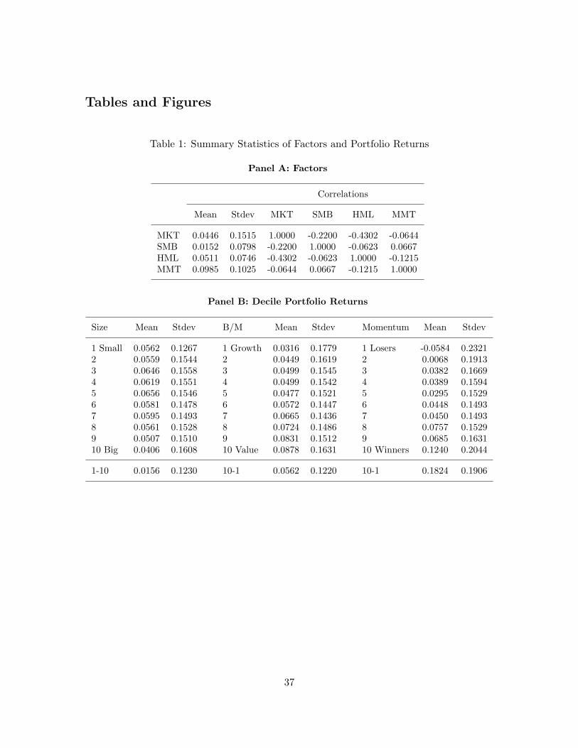
Tables and Figures

Table 1: Summary Statistics of Factors and Portfolio Returns

Panel A: Factors

Correlations

Mean Stdev MKT SMB HML MMT

MKT 0.0446 0.1515 1.0000 -0.2200 -0.4302 -0.0644SMB 0.0152 0.0798 -0.2200 1.0000 -0.0623 0.0667HML 0.0511 0.0746 -0.4302 -0.0623 1.0000 -0.1215MMT 0.0985 0.1025 -0.0644 0.0667 -0.1215 1.0000

Panel B: Decile Portfolio Returns

Size Mean Stdev B/M Mean Stdev Momentum Mean Stdev

1 Small 0.0562 0.1267 1 Growth 0.0316 0.1779 1 Losers -0.0584 0.23212 0.0559 0.1544 2 0.0449 0.1619 2 0.0068 0.19133 0.0646 0.1558 3 0.0499 0.1545 3 0.0382 0.16694 0.0619 0.1551 4 0.0499 0.1542 4 0.0389 0.15945 0.0656 0.1546 5 0.0477 0.1521 5 0.0295 0.15296 0.0581 0.1478 6 0.0572 0.1447 6 0.0448 0.14937 0.0595 0.1493 7 0.0665 0.1436 7 0.0450 0.14938 0.0561 0.1528 8 0.0724 0.1486 8 0.0757 0.15299 0.0507 0.1510 9 0.0831 0.1512 9 0.0685 0.163110 Big 0.0406 0.1608 10 Value 0.0878 0.1631 10 Winners 0.1240 0.2044

1-10 0.0156 0.1230 10-1 0.0562 0.1220 10-1 0.1824 0.1906

37

Table 2: Test of Diagonality of Variance-Covariance Matrix

Model LM Test p-Value

Fixed Time Regression 15185.9766 0.0000Random Time Regression 6974.5703 0.0000

38

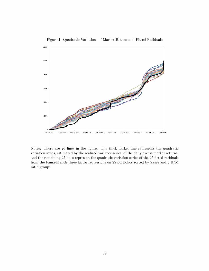
Figure 1: Quadratic Variations of Market Return and Fitted Residuals

Notes: There are 26 lines in the figure. The thick darker line represents the quadraticvariation series, estimated by the realized variance series, of the daily excess market returns,and the remaining 25 lines represent the quadratic variation series of the 25 fitted residualsfrom the Fama-French three factor regressions on 25 portfolios sorted by 5 size and 5 B/Mratio groups.

39

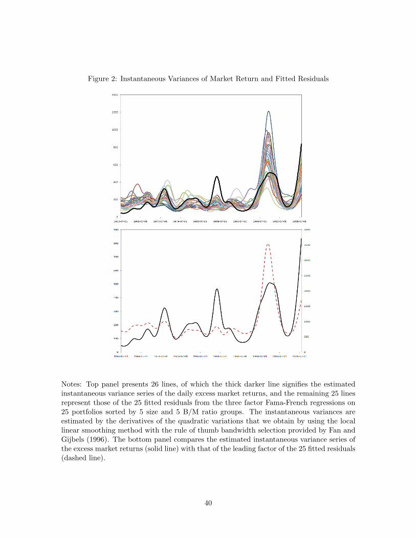
Figure 2: Instantaneous Variances of Market Return and Fitted Residuals

Notes: Top panel presents 26 lines, of which the thick darker line signifies the estimatedinstantaneous variance series of the daily excess market returns, and the remaining 25 linesrepresent those of the 25 fitted residuals from the three factor Fama-French regressions on25 portfolios sorted by 5 size and 5 B/M ratio groups. The instantaneous variances areestimated by the derivatives of the quadratic variations that we obtain by using the locallinear smoothing method with the rule of thumb bandwidth selection provided by Fan andGijbels (1996). The bottom panel compares the estimated instantaneous variance series ofthe excess market returns (solid line) with that of the leading factor of the 25 fitted residuals(dashed line).

40

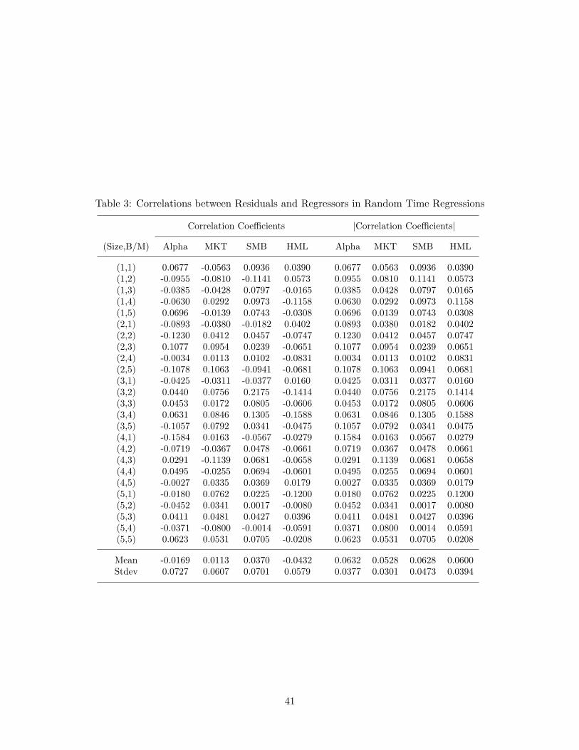
Table 3: Correlations between Residuals and Regressors in Random Time Regressions

Correlation Coefficients |Correlation Coefficients|

(Size,B/M) Alpha MKT SMB HML Alpha MKT SMB HML

(1,1) 0.0677 -0.0563 0.0936 0.0390 0.0677 0.0563 0.0936 0.0390(1,2) -0.0955 -0.0810 -0.1141 0.0573 0.0955 0.0810 0.1141 0.0573(1,3) -0.0385 -0.0428 0.0797 -0.0165 0.0385 0.0428 0.0797 0.0165(1,4) -0.0630 0.0292 0.0973 -0.1158 0.0630 0.0292 0.0973 0.1158(1,5) 0.0696 -0.0139 0.0743 -0.0308 0.0696 0.0139 0.0743 0.0308(2,1) -0.0893 -0.0380 -0.0182 0.0402 0.0893 0.0380 0.0182 0.0402(2,2) -0.1230 0.0412 0.0457 -0.0747 0.1230 0.0412 0.0457 0.0747(2,3) 0.1077 0.0954 0.0239 -0.0651 0.1077 0.0954 0.0239 0.0651(2,4) -0.0034 0.0113 0.0102 -0.0831 0.0034 0.0113 0.0102 0.0831(2,5) -0.1078 0.1063 -0.0941 -0.0681 0.1078 0.1063 0.0941 0.0681(3,1) -0.0425 -0.0311 -0.0377 0.0160 0.0425 0.0311 0.0377 0.0160(3,2) 0.0440 0.0756 0.2175 -0.1414 0.0440 0.0756 0.2175 0.1414(3,3) 0.0453 0.0172 0.0805 -0.0606 0.0453 0.0172 0.0805 0.0606(3,4) 0.0631 0.0846 0.1305 -0.1588 0.0631 0.0846 0.1305 0.1588(3,5) -0.1057 0.0792 0.0341 -0.0475 0.1057 0.0792 0.0341 0.0475(4,1) -0.1584 0.0163 -0.0567 -0.0279 0.1584 0.0163 0.0567 0.0279(4,2) -0.0719 -0.0367 0.0478 -0.0661 0.0719 0.0367 0.0478 0.0661(4,3) 0.0291 -0.1139 0.0681 -0.0658 0.0291 0.1139 0.0681 0.0658(4,4) 0.0495 -0.0255 0.0694 -0.0601 0.0495 0.0255 0.0694 0.0601(4,5) -0.0027 0.0335 0.0369 0.0179 0.0027 0.0335 0.0369 0.0179(5,1) -0.0180 0.0762 0.0225 -0.1200 0.0180 0.0762 0.0225 0.1200(5,2) -0.0452 0.0341 0.0017 -0.0080 0.0452 0.0341 0.0017 0.0080(5,3) 0.0411 0.0481 0.0427 0.0396 0.0411 0.0481 0.0427 0.0396(5,4) -0.0371 -0.0800 -0.0014 -0.0591 0.0371 0.0800 0.0014 0.0591(5,5) 0.0623 0.0531 0.0705 -0.0208 0.0623 0.0531 0.0705 0.0208

Mean -0.0169 0.0113 0.0370 -0.0432 0.0632 0.0528 0.0628 0.0600Stdev 0.0727 0.0607 0.0701 0.0579 0.0377 0.0301 0.0473 0.0394

41

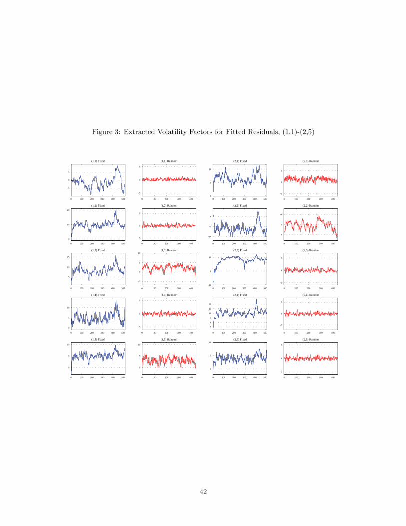
Figure 3: Extracted Volatility Factors for Fitted Residuals, (1,1)-(2,5)

0 100 200 300 400 500

−5

0

5

(1,1) Fixed

0 100 200 300 400

−5

0

5

(1,1) Random

0 100 200 300 400 500

0

10

20

(1,2) Fixed

0 100 200 300 400

−5

0

5

(1,2) Random

0 100 200 300 400 500

5

10

15

(1,3) Fixed

0 100 200 300 400

−5

0

5

10(1,3) Random

0 100 200 300 400 500

0

5

10

(1,4) Fixed

0 100 200 300 400

−5

0

5

(1,4) Random

0 100 200 300 400 500

0

5

10

(1,5) Fixed

0 100 200 300 400

0

5

10

(1,5) Random

0 100 200 300 400 5000

5

10

(2,1) Fixed

0 100 200 300 400

−5

0

5

(2,1) Random

0 100 200 300 400 500

−10

−5

0

(2,2) Fixed

0 100 200 300 400

0

5

10

(2,2) Random

0 100 200 300 400 500−10

0

10

(2,3) Fixed

0 100 200 300 400

−5

0

5

(2,3) Random

0 100 200 300 400 500

−5

0

5

10

15

20

(2,4) Fixed

0 100 200 300 400

−5

0

5

(2,4) Random

0 100 200 300 400 500

0

5

10(2,5) Fixed

0 100 200 300 400

−5

0

5

(2,5) Random

42

Figure 4: Extracted Volatility Factors for Fitted Residuals, (3,1)-(4,5)

0 100 200 300 400 500

5

10

15

(3,1) Fixed

0 100 200 300 400

0

5

10

(3,1) Random

0 100 200 300 400 500

−10

−5

0

(3,2) Fixed

0 100 200 300 400

−5

0

5

(3,2) Random

0 100 200 300 400 500−10

0

10

(3,3) Fixed

0 100 200 300 400−5

0

5

10

(3,3) Random

0 100 200 300 400 500

−10

−5

0

(3,4) Fixed

0 100 200 300 400−5

0

5

(3,4) Random

0 100 200 300 400 500

−5

0

(3,5) Fixed

0 100 200 300 400

0

5

10

(3,5) Random

0 100 200 300 400 500

−10

−5

0

(4,1) Fixed

0 100 200 300 400

0

5

10

(4,1) Random

0 100 200 300 400 500

−10

0

10

(4,2) Fixed

0 100 200 300 400

−5

0

5

(4,2) Random

0 100 200 300 400 500

−10

−5

0

(4,3) Fixed

0 100 200 300 400−5

0

5

10(4,3) Random

0 100 200 300 400 500

−5

0

5

(4,4) Fixed

0 100 200 300 400−5

0

5

10

(4,4) Random

0 100 200 300 400 5000

5

10

15

(4,5) Fixed

0 100 200 300 400

−5

0

5

(4,5) Random

43

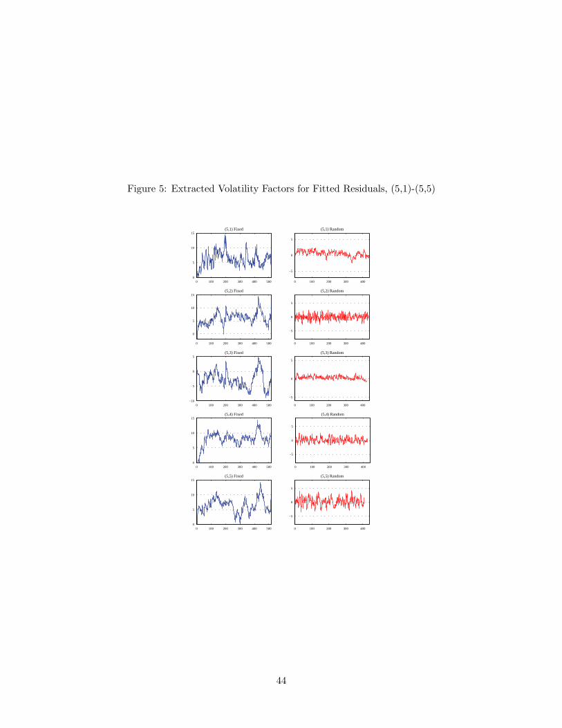
Figure 5: Extracted Volatility Factors for Fitted Residuals, (5,1)-(5,5)

0 100 200 300 400 5000

5

10

15(5,1) Fixed

0 100 200 300 400

−5

0

5

(5,1) Random

0 100 200 300 400 500

0

5

10

15(5,2) Fixed

0 100 200 300 400

−5

0

5

(5,2) Random

0 100 200 300 400 500−10

−5

0

5(5,3) Fixed

0 100 200 300 400

−5

0

5

(5,3) Random

0 100 200 300 400 5000

5

10

15(5,4) Fixed

0 100 200 300 400

−5

0

5

(5,4) Random

0 100 200 300 400 5000

5

10

15(5,5) Fixed

0 100 200 300 400

−5

0

5

(5,5) Random

44

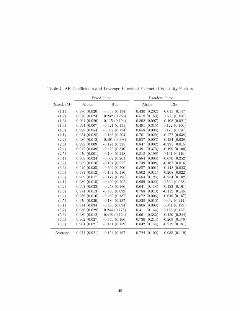
Table 4: AR Coefficients and Leverage Effects of Extracted Volatility Factors

Fixed Time Random Time

(Size,B/M) Alpha Rho Alpha Rho

(1,1) 0.980 (0.020) -0.338 (0.194) 0.430 (0.202) -0.015 (0.147)(1,2) 0.970 (0.024) 0.232 (0.280) 0.518 (0.159) 0.600 (0.166)(1,3) 0.961 (0.029) 0.115 (0.194) 0.892 (0.007) -0.108 (0.021)(1,4) 0.994 (0.007) -0.421 (0.191) 0.491 (0.315) 0.122 (0.160)(1,5) 0.928 (0.054) -0.082 (0.174) 0.858 (0.008) 0.175 (0.020)(2,1) 0.954 (0.028) -0.133 (0.204) 0.701 (0.029) -0.277 (0.038)(2,2) 0.980 (0.012) 0.491 (0.098) 0.957 (0.003) -0.134 (0.028)(2,3) 0.992 (0.009) -0.174 (0.325) 0.847 (0.002) -0.295 (0.015)(2,4) 0.972 (0.039) -0.426 (0.340) 0.491 (0.373) -0.199 (0.100)(2,5) 0.970 (0.001) -0.100 (0.228) 0.518 (0.199) 0.161 (0.119)(3,1) 0.969 (0.024) -0.062 (0.261) 0.884 (0.008) -0.070 (0.252)(3,2) 0.989 (0.010) -0.154 (0.227) 0.739 (0.008) -0.167 (0.016)(3,3) 0.949 (0.035) -0.302 (0.200) 0.857 (0.001) -0.448 (0.023)(3,4) 0.981 (0.012) -0.167 (0.180) 0.802 (0.011) -0.208 (0.022)(3,5) 0.969 (0.017) -0.177 (0.195) 0.584 (0.125) -0.254 (0.182)(4,1) 0.989 (0.015) -0.400 (0.202) 0.959 (0.020) 0.539 (0.023)(4,2) 0.992 (0.023) -0.258 (0.166) 0.641 (0.118) -0.122 (0.161)(4,3) 0.974 (0.013) -0.403 (0.092) 0.788 (0.010) -0.112 (0.145)(4,4) 0.986 (0.016) -0.460 (0.187) 0.872 (0.006) -0.049 (0.157)(4,5) 0.970 (0.020) -0.189 (0.237) 0.828 (0.010) 0.392 (0.214)(5,1) 0.944 (0.034) -0.496 (0.094) 0.808 (0.008) 0.041 (0.199)(5,2) 0.956 (0.029) 0.244 (0.175) 0.411 (0.144) 0.165 (0.155)(5,3) 0.980 (0.012) 0.448 (0.124) 0.661 (0.382) -0.129 (0.244)(5,4) 0.962 (0.027) -0.446 (0.166) 0.730 (0.214) -0.269 (0.178)(5,5) 0.964 (0.021) -0.181 (0.189) 0.842 (0.144) -0.219 (0.181)

Average 0.971 (0.021) -0.154 (0.197) 0.724 (0.100) -0.035 (0.119)

45

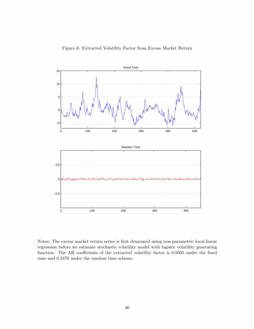
Figure 6: Extracted Volatility Factor from Excess Market Return

0 100 200 300 400 500

−5

0

5

10

15Fixed Time

0 100 200 300 400

−0.5

0

0.5

Random Time

Notes: The excess market return series is first demeaned using non-parametric local-linearregression before we estimate stochastic volatility model with logistic volatility generatingfunction. The AR coefficients of the extracted volatility factor is 0.9505 under the fixedtime and 0.2476 under the random time scheme.

46

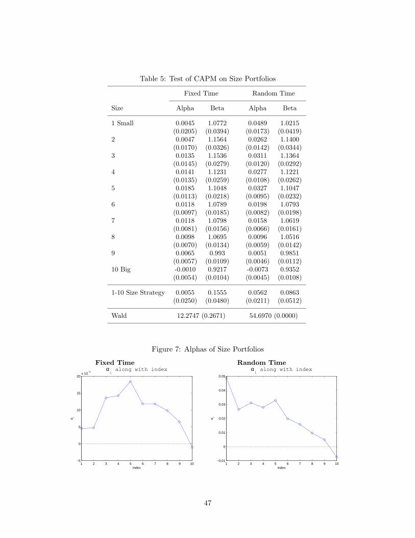
Table 5: Test of CAPM on Size Portfolios

Fixed Time Random Time

Size Alpha Beta Alpha Beta

1 Small 0.0045 1.0772 0.0489 1.0215(0.0205) (0.0394) (0.0173) (0.0419)

2 0.0047 1.1564 0.0262 1.1400(0.0170) (0.0326) (0.0142) (0.0344)

3 0.0135 1.1536 0.0311 1.1364(0.0145) (0.0279) (0.0120) (0.0292)

4 0.0141 1.1231 0.0277 1.1221(0.0135) (0.0259) (0.0108) (0.0262)

5 0.0185 1.1048 0.0327 1.1047(0.0113) (0.0218) (0.0095) (0.0232)

6 0.0118 1.0789 0.0198 1.0793(0.0097) (0.0185) (0.0082) (0.0198)

7 0.0118 1.0798 0.0158 1.0619(0.0081) (0.0156) (0.0066) (0.0161)

8 0.0098 1.0695 0.0096 1.0516(0.0070) (0.0134) (0.0059) (0.0142)

9 0.0065 0.993 0.0051 0.9851(0.0057) (0.0109) (0.0046) (0.0112)

10 Big -0.0010 0.9217 -0.0073 0.9352(0.0054) (0.0104) (0.0045) (0.0108)

1-10 Size Strategy 0.0055 0.1555 0.0562 0.0863(0.0250) (0.0480) (0.0211) (0.0512)

Wald 12.2747 (0.2671) 54.6970 (0.0000)

Figure 7: Alphas of Size Portfolios

Fixed Time Random Timeαi along with index

index

α i

1 2 3 4 5 6 7 8 9 10−5

0

5

10

15

20x 10

−3αi along with index

index

α i

1 2 3 4 5 6 7 8 9 10−0.01

0

0.01

0.02

0.03

0.04

0.05

47

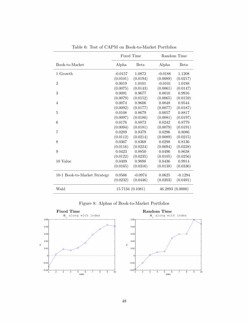
Table 6: Test of CAPM on Book-to-Market Portfolios

Fixed Time Random Time

Book-to-Market Alpha Beta Alpha Beta

1 Growth -0.0157 1.0872 -0.0188 1.1208(0.0101) (0.0194) (0.0089) (0.0217)

2 0.0019 1.0101 -0.0101 1.0188(0.0075) (0.0143) (0.0061) (0.0147)

3 0.0091 0.9677 0.0010 0.9916(0.0079) (0.0152) (0.0065) (0.0159)

4 0.0074 0.9606 0.0048 0.9544(0.0092) (0.0177) (0.0077) (0.0187)

5 0.0108 0.8679 0.0057 0.8817(0.0097) (0.0186) (0.0081) (0.0197)

6 0.0176 0.8873 0.0242 0.8779(0.0094) (0.0181) (0.0079) (0.0191)

7 0.0289 0.8379 0.0296 0.8086(0.0112) (0.0214) (0.0089) (0.0215)

8 0.0367 0.8368 0.0298 0.8136(0.0116) (0.0224) (0.0094) (0.0228)

9 0.0423 0.8850 0.0496 0.8638(0.0122) (0.0235) (0.0105) (0.0256)

10 Value 0.0409 0.9898 0.0436 0.9914(0.0165) (0.0316) (0.0138) (0.0336)

10-1 Book-to-Market Strategy 0.0566 -0.0974 0.0625 -0.1294(0.0232) (0.0446) (0.0203) (0.0491)

Wald 15.7134 (0.1081) 46.2893 (0.0000)

Figure 8: Alphas of Book-to-Market Portfolios

Fixed Time Random Timeαi along with index

index

α i

1 2 3 4 5 6 7 8 9 10−0.02

−0.01

0

0.01

0.02

0.03

0.04

0.05

αi along with index

index

α i

1 2 3 4 5 6 7 8 9 10−0.02

−0.01

0

0.01

0.02

0.03

0.04

0.05

48

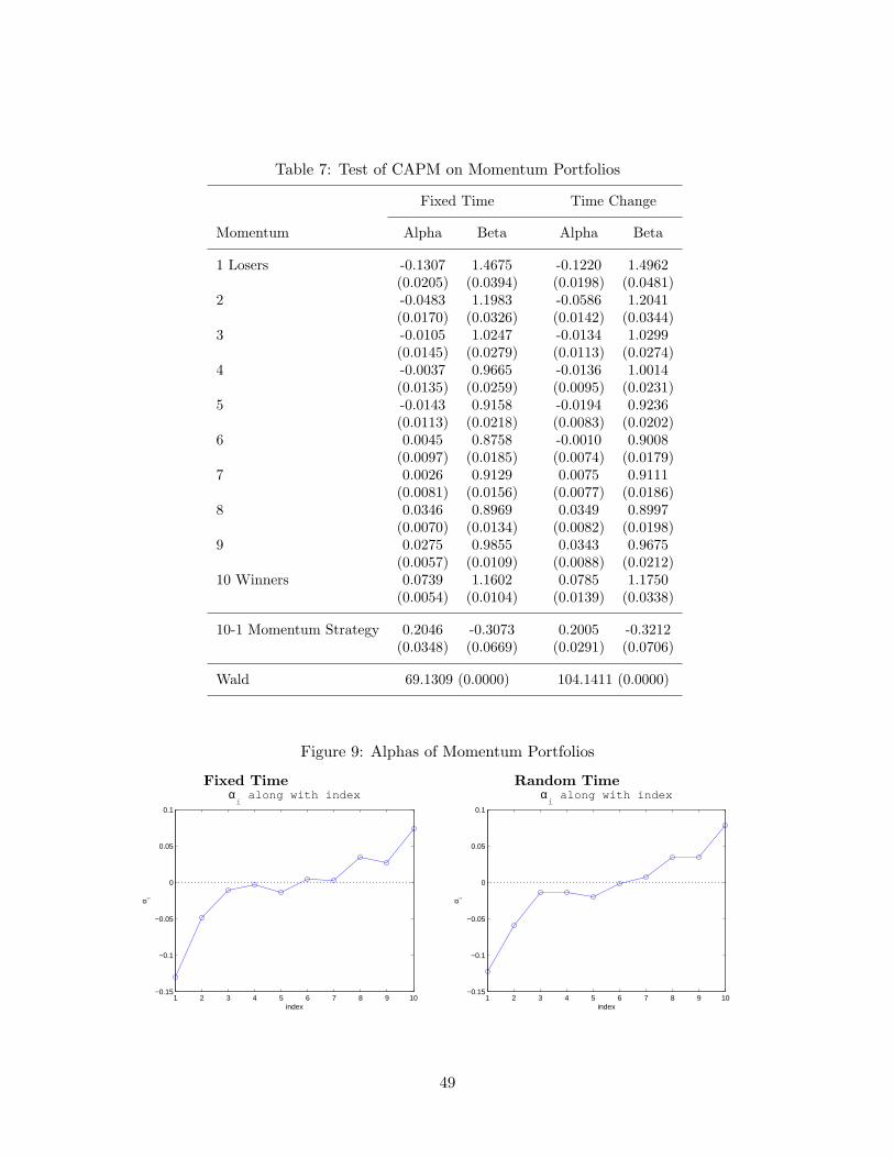
Table 7: Test of CAPM on Momentum Portfolios

Fixed Time Time Change

Momentum Alpha Beta Alpha Beta

1 Losers -0.1307 1.4675 -0.1220 1.4962(0.0205) (0.0394) (0.0198) (0.0481)

2 -0.0483 1.1983 -0.0586 1.2041(0.0170) (0.0326) (0.0142) (0.0344)

3 -0.0105 1.0247 -0.0134 1.0299(0.0145) (0.0279) (0.0113) (0.0274)

4 -0.0037 0.9665 -0.0136 1.0014(0.0135) (0.0259) (0.0095) (0.0231)

5 -0.0143 0.9158 -0.0194 0.9236(0.0113) (0.0218) (0.0083) (0.0202)

6 0.0045 0.8758 -0.0010 0.9008(0.0097) (0.0185) (0.0074) (0.0179)

7 0.0026 0.9129 0.0075 0.9111(0.0081) (0.0156) (0.0077) (0.0186)

8 0.0346 0.8969 0.0349 0.8997(0.0070) (0.0134) (0.0082) (0.0198)

9 0.0275 0.9855 0.0343 0.9675(0.0057) (0.0109) (0.0088) (0.0212)

10 Winners 0.0739 1.1602 0.0785 1.1750(0.0054) (0.0104) (0.0139) (0.0338)

10-1 Momentum Strategy 0.2046 -0.3073 0.2005 -0.3212(0.0348) (0.0669) (0.0291) (0.0706)

Wald 69.1309 (0.0000) 104.1411 (0.0000)

Figure 9: Alphas of Momentum Portfolios

Fixed Time Random Timeαi along with index

index

α i

1 2 3 4 5 6 7 8 9 10−0.15

−0.1

−0.05

0

0.05

0.1

αi along with index

index

α i

1 2 3 4 5 6 7 8 9 10−0.15

−0.1

−0.05

0

0.05

0.1

49

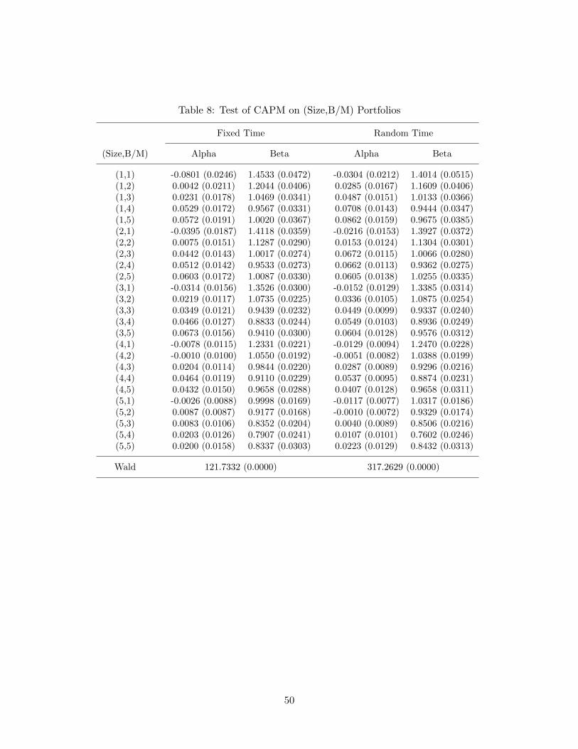
Table 8: Test of CAPM on (Size,B/M) Portfolios

Fixed Time Random Time

(Size,B/M) Alpha Beta Alpha Beta

(1,1) -0.0801 (0.0246) 1.4533 (0.0472) -0.0304 (0.0212) 1.4014 (0.0515)(1,2) 0.0042 (0.0211) 1.2044 (0.0406) 0.0285 (0.0167) 1.1609 (0.0406)(1,3) 0.0231 (0.0178) 1.0469 (0.0341) 0.0487 (0.0151) 1.0133 (0.0366)(1,4) 0.0529 (0.0172) 0.9567 (0.0331) 0.0708 (0.0143) 0.9444 (0.0347)(1,5) 0.0572 (0.0191) 1.0020 (0.0367) 0.0862 (0.0159) 0.9675 (0.0385)(2,1) -0.0395 (0.0187) 1.4118 (0.0359) -0.0216 (0.0153) 1.3927 (0.0372)(2,2) 0.0075 (0.0151) 1.1287 (0.0290) 0.0153 (0.0124) 1.1304 (0.0301)(2,3) 0.0442 (0.0143) 1.0017 (0.0274) 0.0672 (0.0115) 1.0066 (0.0280)(2,4) 0.0512 (0.0142) 0.9533 (0.0273) 0.0662 (0.0113) 0.9362 (0.0275)(2,5) 0.0603 (0.0172) 1.0087 (0.0330) 0.0605 (0.0138) 1.0255 (0.0335)(3,1) -0.0314 (0.0156) 1.3526 (0.0300) -0.0152 (0.0129) 1.3385 (0.0314)(3,2) 0.0219 (0.0117) 1.0735 (0.0225) 0.0336 (0.0105) 1.0875 (0.0254)(3,3) 0.0349 (0.0121) 0.9439 (0.0232) 0.0449 (0.0099) 0.9337 (0.0240)(3,4) 0.0466 (0.0127) 0.8833 (0.0244) 0.0549 (0.0103) 0.8936 (0.0249)(3,5) 0.0673 (0.0156) 0.9410 (0.0300) 0.0604 (0.0128) 0.9576 (0.0312)(4,1) -0.0078 (0.0115) 1.2331 (0.0221) -0.0129 (0.0094) 1.2470 (0.0228)(4,2) -0.0010 (0.0100) 1.0550 (0.0192) -0.0051 (0.0082) 1.0388 (0.0199)(4,3) 0.0204 (0.0114) 0.9844 (0.0220) 0.0287 (0.0089) 0.9296 (0.0216)(4,4) 0.0464 (0.0119) 0.9110 (0.0229) 0.0537 (0.0095) 0.8874 (0.0231)(4,5) 0.0432 (0.0150) 0.9658 (0.0288) 0.0407 (0.0128) 0.9658 (0.0311)(5,1) -0.0026 (0.0088) 0.9998 (0.0169) -0.0117 (0.0077) 1.0317 (0.0186)(5,2) 0.0087 (0.0087) 0.9177 (0.0168) -0.0010 (0.0072) 0.9329 (0.0174)(5,3) 0.0083 (0.0106) 0.8352 (0.0204) 0.0040 (0.0089) 0.8506 (0.0216)(5,4) 0.0203 (0.0126) 0.7907 (0.0241) 0.0107 (0.0101) 0.7602 (0.0246)(5,5) 0.0200 (0.0158) 0.8337 (0.0303) 0.0223 (0.0129) 0.8432 (0.0313)

Wald 121.7332 (0.0000) 317.2629 (0.0000)

50

Figure 10: Alphas of (Size,B/M) Portfolios

Fixed Time

0 5 10 15 20 25−0.1

−0.08

−0.06

−0.04

−0.02

0

0.02

0.04

0.06

0.08

index

α i

αi along the index

size

α i

Fixing B/M

1 2 3 4 5−0.1

−0.08

−0.06

−0.04

−0.02

0

0.02

0.04

0.06

0.08

B/M=1B/M=2B/M=3B/M=4B/M=5

B/M

α i

Fixing Size

1 2 3 4 5−0.1

−0.08

−0.06

−0.04

−0.02

0

0.02

0.04

0.06

0.08

size=1size=2size=3size=4size=5

Random Time

0 5 10 15 20 25−0.04

−0.02

0

0.02

0.04

0.06

0.08

0.1

index

α i

αi along the index

size

α i

Fixing B/M

1 2 3 4 5−0.04

−0.02

0

0.02

0.04

0.06

0.08

0.1B/M=1B/M=2B/M=3B/M=4B/M=5

B/M

α i

Fixing Size

1 2 3 4 5−0.04

−0.02

0

0.02

0.04

0.06

0.08

0.1size=1size=2size=3size=4size=5

51

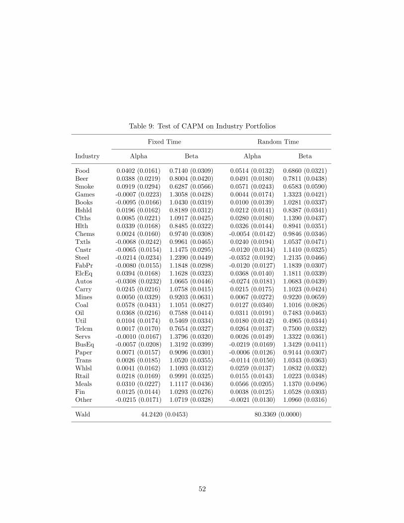
Table 9: Test of CAPM on Industry Portfolios

Fixed Time Random Time

Industry Alpha Beta Alpha Beta

Food 0.0402 (0.0161) 0.7140 (0.0309) 0.0514 (0.0132) 0.6860 (0.0321)Beer 0.0388 (0.0219) 0.8004 (0.0420) 0.0491 (0.0180) 0.7811 (0.0438)Smoke 0.0919 (0.0294) 0.6287 (0.0566) 0.0571 (0.0243) 0.6583 (0.0590)Games -0.0007 (0.0223) 1.3058 (0.0428) 0.0044 (0.0174) 1.3323 (0.0421)Books -0.0095 (0.0166) 1.0430 (0.0319) 0.0100 (0.0139) 1.0281 (0.0337)Hshld 0.0196 (0.0162) 0.8189 (0.0312) 0.0212 (0.0141) 0.8387 (0.0341)Clths 0.0085 (0.0221) 1.0917 (0.0425) 0.0280 (0.0180) 1.1390 (0.0437)Hlth 0.0339 (0.0168) 0.8485 (0.0322) 0.0326 (0.0144) 0.8941 (0.0351)Chems 0.0024 (0.0160) 0.9740 (0.0308) -0.0054 (0.0142) 0.9846 (0.0346)Txtls -0.0068 (0.0242) 0.9961 (0.0465) 0.0240 (0.0194) 1.0537 (0.0471)Cnstr -0.0065 (0.0154) 1.1475 (0.0295) -0.0120 (0.0134) 1.1410 (0.0325)Steel -0.0214 (0.0234) 1.2390 (0.0449) -0.0352 (0.0192) 1.2135 (0.0466)FabPr -0.0080 (0.0155) 1.1848 (0.0298) -0.0120 (0.0127) 1.1839 (0.0307)ElcEq 0.0394 (0.0168) 1.1628 (0.0323) 0.0368 (0.0140) 1.1811 (0.0339)Autos -0.0308 (0.0232) 1.0665 (0.0446) -0.0274 (0.0181) 1.0683 (0.0439)Carry 0.0245 (0.0216) 1.0758 (0.0415) 0.0215 (0.0175) 1.1023 (0.0424)Mines 0.0050 (0.0329) 0.9203 (0.0631) 0.0067 (0.0272) 0.9220 (0.0659)Coal 0.0578 (0.0431) 1.1051 (0.0827) 0.0127 (0.0340) 1.1016 (0.0826)Oil 0.0368 (0.0216) 0.7588 (0.0414) 0.0311 (0.0191) 0.7483 (0.0463)Util 0.0104 (0.0174) 0.5469 (0.0334) 0.0180 (0.0142) 0.4965 (0.0344)Telcm 0.0017 (0.0170) 0.7654 (0.0327) 0.0264 (0.0137) 0.7500 (0.0332)Servs -0.0010 (0.0167) 1.3796 (0.0320) 0.0026 (0.0149) 1.3322 (0.0361)BusEq -0.0057 (0.0208) 1.3192 (0.0399) -0.0219 (0.0169) 1.3429 (0.0411)Paper 0.0071 (0.0157) 0.9096 (0.0301) -0.0006 (0.0126) 0.9144 (0.0307)Trans 0.0026 (0.0185) 1.0520 (0.0355) -0.0114 (0.0150) 1.0343 (0.0363)Whlsl 0.0041 (0.0162) 1.1093 (0.0312) 0.0259 (0.0137) 1.0832 (0.0332)Rtail 0.0218 (0.0169) 0.9991 (0.0325) 0.0155 (0.0143) 1.0223 (0.0348)Meals 0.0310 (0.0227) 1.1117 (0.0436) 0.0566 (0.0205) 1.1370 (0.0496)Fin 0.0125 (0.0144) 1.0293 (0.0276) 0.0038 (0.0125) 1.0528 (0.0303)Other -0.0215 (0.0171) 1.0719 (0.0328) -0.0021 (0.0130) 1.0960 (0.0316)

Wald 44.2420 (0.0453) 80.3369 (0.0000)

52

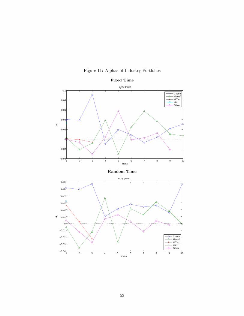
Figure 11: Alphas of Industry Portfolios

Fixed Time

αi by group

index

α i

1 2 3 4 5 6 7 8 9 10−0.04

−0.02

0

0.02

0.04

0.06

0.08

0.1CnsmrManufHiTecHlthOther

Random Time

αi by group

index

α i

1 2 3 4 5 6 7 8 9 10−0.04

−0.03

−0.02

−0.01

0

0.01

0.02

0.03

0.04

0.05

0.06

CnsmrManufHiTecHlthOther

53

Table 10: Test of Two-Factor Model on Size Portfolios

Fixed Time Random Time

Size Alpha Beta MKT Beta SMB Alpha Beta MKT Beta SMB

1 Small -0.0038 0.8466 1.1876 0.0109 0.8010 1.2398(0.0095) (0.0189) (0.0272) (0.0073) (0.0184) (0.0276)

2 -0.0026 0.9551 1.0362 -0.006 0.9534 1.049(0.0060) (0.0121) (0.0174) (0.0051) (0.0127) (0.0191)

3 0.0074 0.9832 0.8771 0.0039 0.9790 0.8847(0.0056) (0.0112) (0.0161) (0.0045) (0.0111) (0.0167)

4 0.0086 0.9682 0.7975 0.0036 0.9828 0.7831(0.0057) (0.0114) (0.0164) (0.0043) (0.0109) (0.0163)

5 0.0139 0.9799 0.6434 0.0123 0.9863 0.6659(0.0056) (0.0112) (0.0162) (0.0045) (0.0113) (0.0170)

6 0.0085 0.9872 0.4718 0.0046 0.9908 0.4978(0.0064) (0.0128) (0.0184) (0.0052) (0.0131) (0.0197)

7 0.0093 1.0119 0.3494 0.0047 0.9976 0.3617(0.0061) (0.0122) (0.0175) (0.0048) (0.0121) (0.0181)

8 0.0082 1.0249 0.2296 0.0026 1.0112 0.2271(0.0060) (0.0120) (0.0173) (0.0052) (0.0129) (0.0194)

9 0.0063 0.9852 0.0402 0.0043 0.9808 0.0240(0.0057) (0.0113) (0.0163) (0.0046) (0.0116) (0.0174)

10 Big 0.0010 0.9788 -0.2942 0.0016 0.9867 -0.2891(0.0030) (0.0060) (0.0087) (0.0026) (0.0064) (0.0096)

1-10 Size Strategy -0.0049 -0.1323 -1.4818 0.0092 -0.1857 1.5290(0.0250) (0.0500) (0.0719) (0.0212) (0.0531) (0.0797)

Wald 12.0613 (0.2810) 31.3234 (0.0005)

54

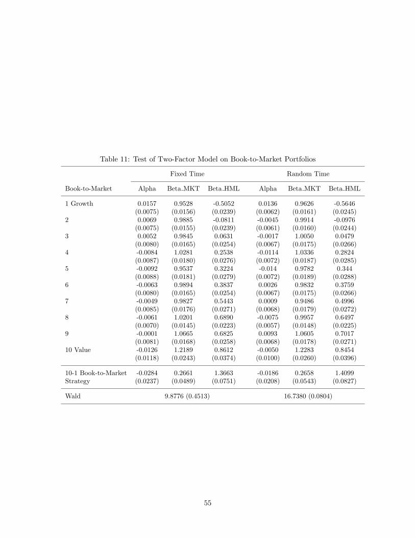
Table 11: Test of Two-Factor Model on Book-to-Market Portfolios

Fixed Time Random Time

Book-to-Market Alpha Beta MKT Beta HML Alpha Beta MKT Beta HML

1 Growth 0.0157 0.9528 -0.5052 0.0136 0.9626 -0.5646(0.0075) (0.0156) (0.0239) (0.0062) (0.0161) (0.0245)

2 0.0069 0.9885 -0.0811 -0.0045 0.9914 -0.0976(0.0075) (0.0155) (0.0239) (0.0061) (0.0160) (0.0244)

3 0.0052 0.9845 0.0631 -0.0017 1.0050 0.0479(0.0080) (0.0165) (0.0254) (0.0067) (0.0175) (0.0266)

4 -0.0084 1.0281 0.2538 -0.0114 1.0336 0.2824(0.0087) (0.0180) (0.0276) (0.0072) (0.0187) (0.0285)

5 -0.0092 0.9537 0.3224 -0.014 0.9782 0.344(0.0088) (0.0181) (0.0279) (0.0072) (0.0189) (0.0288)

6 -0.0063 0.9894 0.3837 0.0026 0.9832 0.3759(0.0080) (0.0165) (0.0254) (0.0067) (0.0175) (0.0266)

7 -0.0049 0.9827 0.5443 0.0009 0.9486 0.4996(0.0085) (0.0176) (0.0271) (0.0068) (0.0179) (0.0272)

8 -0.0061 1.0201 0.6890 -0.0075 0.9957 0.6497(0.0070) (0.0145) (0.0223) (0.0057) (0.0148) (0.0225)

9 -0.0001 1.0665 0.6825 0.0093 1.0605 0.7017(0.0081) (0.0168) (0.0258) (0.0068) (0.0178) (0.0271)

10 Value -0.0126 1.2189 0.8612 -0.0050 1.2283 0.8454(0.0118) (0.0243) (0.0374) (0.0100) (0.0260) (0.0396)

10-1 Book-to-Market -0.0284 0.2661 1.3663 -0.0186 0.2658 1.4099Strategy (0.0237) (0.0489) (0.0751) (0.0208) (0.0543) (0.0827)

Wald 9.8776 (0.4513) 16.7380 (0.0804)

55

Table 12: Test of Two-Factor Model on Momentum Portfolios

Fixed Time Random Time

Momentum Alpha Beta MKT Beta MMT Alpha Beta MKT Beta MMT

1 Losers -0.0396 1.3428 -0.8501 -0.0238 1.3614 -0.9089(0.0147) (0.0279) (0.0296) (0.0133) (0.0314) (0.0364)

2 0.0287 1.0928 -0.7188 0.0203 1.0957 -0.7310(0.0094) (0.0178) (0.0188) (0.0075) (0.0177) (0.0205)

3 0.0454 0.9482 -0.5216 0.0444 0.9506 -0.5348(0.0090) (0.0171) (0.0181) (0.0072) (0.0170) (0.0197)

4 0.0337 0.9152 -0.3498 0.0241 0.9495 -0.3494(0.0094) (0.0178) (0.0189) (0.0079) (0.0185) (0.0215)

5 0.0111 0.8810 -0.2369 0.0035 0.8922 -0.2118(0.0098) (0.0186) (0.0197) (0.0079) (0.0186) (0.0215)

6 0.0115 0.8662 -0.0653 0.0059 0.8913 -0.0638(0.0096) (0.0183) (0.0194) (0.0077) (0.0180) (0.0209)

7 -0.0043 0.9224 0.0645 -0.0017 0.9236 0.0848(0.0089) (0.0168) (0.0178) (0.0079) (0.0186) (0.0215)

8 0.0094 0.9315 0.2358 0.0100 0.9339 0.2309(0.0095) (0.0180) (0.0191) (0.0075) (0.0178) (0.0206)

9 -0.0080 1.0341 0.3312 -0.0030 1.0186 0.3448(0.0084) (0.0159) (0.0169) (0.0069) (0.0162) (0.0188)

10 Winners 0.0070 1.2518 0.6244 0.0116 1.2669 0.6195(0.0121) (0.0230) (0.0244) (0.0097) (0.0229) (0.0266)

10-1 Momentum Strategy 0.0465 -0.0910 1.4745 0.0354 -0.0945 1.5283(0.0357) (0.0677) (0.0718) (0.0305) (0.0717) (0.0831)

Wald 53.4570 (0.0000) 69.3201 (0.0000)

56

Table 13: Test of Fama-French Three-Factor Model (Fixed Time)

Fixed Time

(Size,B/M) Alpha Beta MKT Beta SMB Beta HML

(1,1) -0.0714 (0.0115) 1.1092 (0.0242) 1.3694 (0.0327) -0.2936 (0.0367)(1,2) -0.0107 (0.0084) 0.9804 (0.0176) 1.2834 (0.0238) 0.0949 (0.0267)(1,3) -0.0043 (0.0070) 0.9231 (0.0147) 1.0747 (0.0199) 0.3192 (0.0224)(1,4) 0.0178 (0.0070) 0.8809 (0.0148) 1.0080 (0.0200) 0.4508 (0.0225)(1,5) 0.0074 (0.0073) 0.9737 (0.0155) 1.0771 (0.0209) 0.6798 (0.0235)(2,1) -0.0234 (0.0087) 1.1208 (0.0184) 0.9896 (0.0249) -0.3714 (0.0280)(2,2) -0.0089 (0.0076) 1.0048 (0.0161) 0.8668 (0.0217) 0.1671 (0.0244)(2,3) 0.0137 (0.0073) 0.9580 (0.0154) 0.7772 (0.0208) 0.4028 (0.0234)(2,4) 0.0100 (0.0069) 0.9708 (0.0145) 0.7102 (0.0196) 0.5842 (0.0221)(2,5) 0.0065 (0.0074) 1.0467 (0.0155) 0.8581 (0.0210) 0.7691 (0.0236)(3,1) -0.0095 (0.0082) 1.0944 (0.0172) 0.7330 (0.0232) -0.4356 (0.0261)(3,2) 0.0058 (0.0087) 1.0242 (0.0182) 0.5264 (0.0246) 0.1990 (0.0277)(3,3) 0.0017 (0.0085) 0.9869 (0.0179) 0.4431 (0.0242) 0.4850 (0.0272)(3,4) 0.0037 (0.0082) 0.9800 (0.0172) 0.3885 (0.0232) 0.6469 (0.0261)(3,5) 0.0143 (0.0095) 1.0495 (0.0200) 0.5287 (0.0270) 0.7936 (0.0304)(4,1) 0.0160 (0.0079) 1.0492 (0.0166) 0.3656 (0.0224) -0.4244 (0.0252)(4,2) -0.0180 (0.0092) 1.0811 (0.0194) 0.2064 (0.0262) 0.2487 (0.0295)(4,3) -0.0114 (0.0094) 1.0844 (0.0198) 0.1621 (0.0267) 0.4940 (0.0301)(4,4) 0.0069 (0.0086) 1.0330 (0.0181) 0.2090 (0.0245) 0.6110 (0.0275)(4,5) -0.0085 (0.0104) 1.1331 (0.0219) 0.2414 (0.0296) 0.8050 (0.0333)(5,1) 0.0228 (0.0065) 0.9505 (0.0137) -0.2645 (0.0185) -0.3786 (0.0208)(5,2) 0.0029 (0.0079) 0.9935 (0.0167) -0.2270 (0.0226) 0.1191 (0.0254)(5,3) -0.0083 (0.0091) 0.9611 (0.0191) -0.2432 (0.0258) 0.2957 (0.0290)(5,4) -0.0181 (0.0080) 1.0051 (0.0168) -0.2246 (0.0228) 0.6419 (0.0256)(5,5) -0.0285 (0.0115) 1.0631 (0.0243) -0.0982 (0.0328) 0.7906 (0.0369)

Wald 95.5585 (0.0000)

57

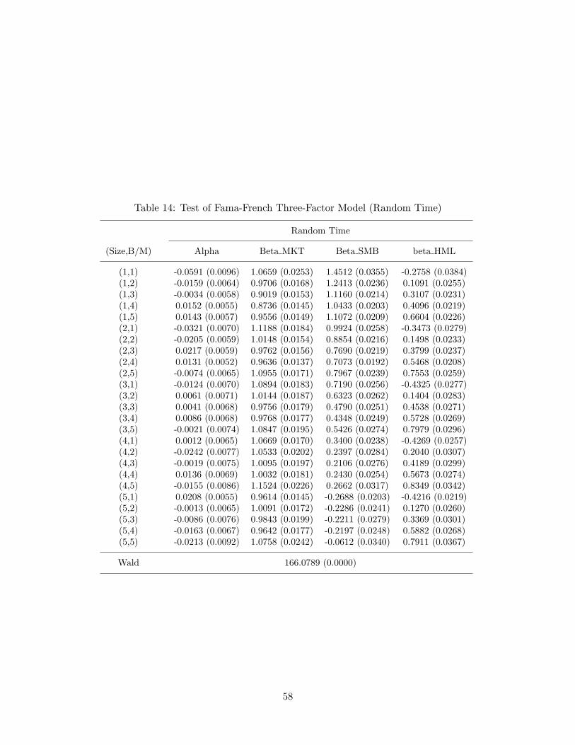
Table 14: Test of Fama-French Three-Factor Model (Random Time)

Random Time

(Size,B/M) Alpha Beta MKT Beta SMB beta HML

(1,1) -0.0591 (0.0096) 1.0659 (0.0253) 1.4512 (0.0355) -0.2758 (0.0384)(1,2) -0.0159 (0.0064) 0.9706 (0.0168) 1.2413 (0.0236) 0.1091 (0.0255)(1,3) -0.0034 (0.0058) 0.9019 (0.0153) 1.1160 (0.0214) 0.3107 (0.0231)(1,4) 0.0152 (0.0055) 0.8736 (0.0145) 1.0433 (0.0203) 0.4096 (0.0219)(1,5) 0.0143 (0.0057) 0.9556 (0.0149) 1.1072 (0.0209) 0.6604 (0.0226)(2,1) -0.0321 (0.0070) 1.1188 (0.0184) 0.9924 (0.0258) -0.3473 (0.0279)(2,2) -0.0205 (0.0059) 1.0148 (0.0154) 0.8854 (0.0216) 0.1498 (0.0233)(2,3) 0.0217 (0.0059) 0.9762 (0.0156) 0.7690 (0.0219) 0.3799 (0.0237)(2,4) 0.0131 (0.0052) 0.9636 (0.0137) 0.7073 (0.0192) 0.5468 (0.0208)(2,5) -0.0074 (0.0065) 1.0955 (0.0171) 0.7967 (0.0239) 0.7553 (0.0259)(3,1) -0.0124 (0.0070) 1.0894 (0.0183) 0.7190 (0.0256) -0.4325 (0.0277)(3,2) 0.0061 (0.0071) 1.0144 (0.0187) 0.6323 (0.0262) 0.1404 (0.0283)(3,3) 0.0041 (0.0068) 0.9756 (0.0179) 0.4790 (0.0251) 0.4538 (0.0271)(3,4) 0.0086 (0.0068) 0.9768 (0.0177) 0.4348 (0.0249) 0.5728 (0.0269)(3,5) -0.0021 (0.0074) 1.0847 (0.0195) 0.5426 (0.0274) 0.7979 (0.0296)(4,1) 0.0012 (0.0065) 1.0669 (0.0170) 0.3400 (0.0238) -0.4269 (0.0257)(4,2) -0.0242 (0.0077) 1.0533 (0.0202) 0.2397 (0.0284) 0.2040 (0.0307)(4,3) -0.0019 (0.0075) 1.0095 (0.0197) 0.2106 (0.0276) 0.4189 (0.0299)(4,4) 0.0136 (0.0069) 1.0032 (0.0181) 0.2430 (0.0254) 0.5673 (0.0274)(4,5) -0.0155 (0.0086) 1.1524 (0.0226) 0.2662 (0.0317) 0.8349 (0.0342)(5,1) 0.0208 (0.0055) 0.9614 (0.0145) -0.2688 (0.0203) -0.4216 (0.0219)(5,2) -0.0013 (0.0065) 1.0091 (0.0172) -0.2286 (0.0241) 0.1270 (0.0260)(5,3) -0.0086 (0.0076) 0.9843 (0.0199) -0.2211 (0.0279) 0.3369 (0.0301)(5,4) -0.0163 (0.0067) 0.9642 (0.0177) -0.2197 (0.0248) 0.5882 (0.0268)(5,5) -0.0213 (0.0092) 1.0758 (0.0242) -0.0612 (0.0340) 0.7911 (0.0367)

Wald 166.0789 (0.0000)

58

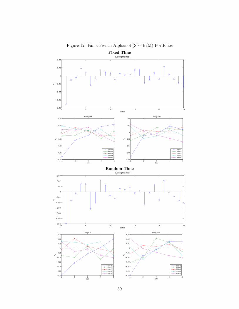
Figure 12: Fama-French Alphas of (Size,B/M) Portfolios

Fixed Time

0 5 10 15 20 25−0.08

−0.06

−0.04

−0.02

0

0.02

0.04

index

α i

αi along the index

size

α i

Fixing B/M

1 2 3 4 5−0.08

−0.06

−0.04

−0.02

0

0.02

0.04

B/M=1B/M=2B/M=3B/M=4B/M=5

B/M

α i

Fixing Size

1 2 3 4 5−0.08

−0.06

−0.04

−0.02

0

0.02

0.04

size=1size=2size=3size=4size=5

Random Time

0 5 10 15 20 25−0.06

−0.05

−0.04

−0.03

−0.02

−0.01

0

0.01

0.02

0.03

index

α i

αi along the index

size

α i

Fixing B/M

1 2 3 4 5−0.06

−0.05

−0.04

−0.03

−0.02

−0.01

0

0.01

0.02

0.03

B/M=1B/M=2B/M=3B/M=4B/M=5

B/M

α i

Fixing Size

1 2 3 4 5−0.06

−0.05

−0.04

−0.03

−0.02

−0.01

0

0.01

0.02

0.03

size=1size=2size=3size=4size=5

59

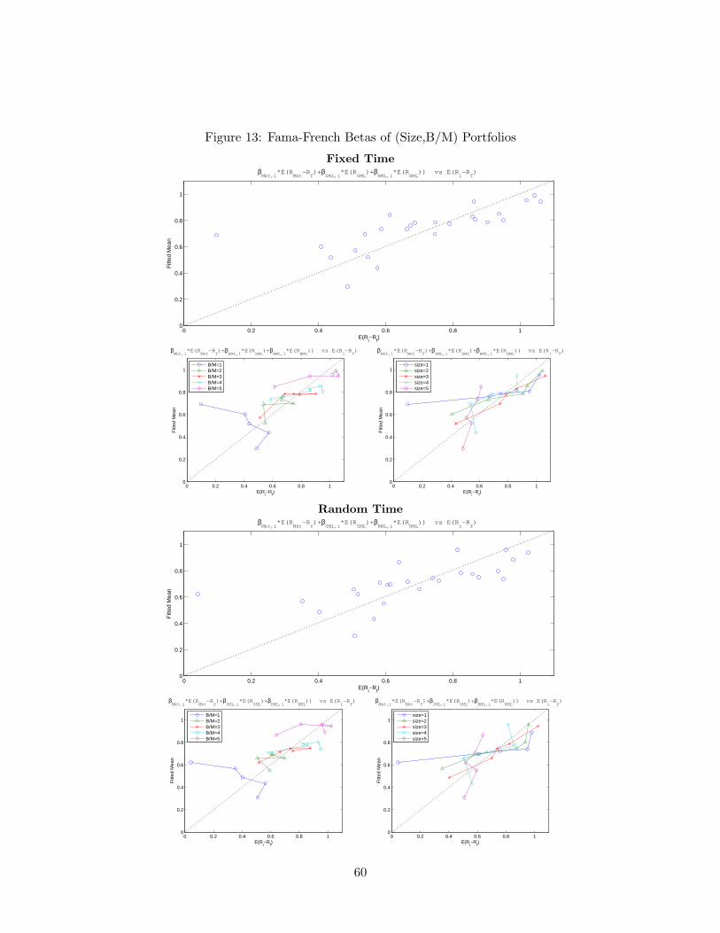
Figure 13: Fama-French Betas of (Size,B/M) Portfolios

Fixed Time

0 0.2 0.4 0.6 0.8 10

0.2

0.4

0.6

0.8

1

βMkt,i

*E(RMkt

−Rf)+ β

SML,i*E(R

SML)+ β

HML,i*E(R

HML)) vs E(R

i−R

f)

E(Ri−R

f)

Fitt

ed M

ean

0 0.2 0.4 0.6 0.8 10

0.2

0.4

0.6

0.8

1

βMkt,i

*E(RMkt

−Rf)+ β

SML,i*E(R

SML)+ β

HML,i*E(R

HML)) vs E(R

i−R

f)

E(Ri−R

f)

Fitt

ed M

ean

B/M=1B/M=2B/M=3B/M=4B/M=5

0 0.2 0.4 0.6 0.8 10

0.2

0.4

0.6

0.8

1

βMkt,i

*E(RMkt

−Rf)+ β

SML,i*E(R

SML)+ β

HML,i*E(R

HML)) vs E(R

i−R

f)

E(Ri−R

f)

Fitt

ed M

ean

size=1size=2size=3size=4size=5

Random Time

0 0.2 0.4 0.6 0.8 10

0.2

0.4

0.6

0.8

1

βMkt,i

*E(RMkt

−Rf)+ β

SML,i*E(R

SML)+ β

HML,i*E(R

HML)) vs E(R

i−R

f)

E(Ri−R

f)

Fitt

ed M

ean

0 0.2 0.4 0.6 0.8 10

0.2

0.4

0.6

0.8

1

βMkt,i

*E(RMkt

−Rf)+ β

SML,i*E(R

SML)+ β

HML,i*E(R

HML)) vs E(R

i−R

f)

E(Ri−R

f)

Fitt

ed M

ean

B/M=1B/M=2B/M=3B/M=4B/M=5

0 0.2 0.4 0.6 0.8 10

0.2

0.4

0.6

0.8

1

βMkt,i

*E(RMkt

−Rf)+ β

SML,i*E(R

SML)+ β

HML,i*E(R

HML)) vs E(R

i−R

f)

E(Ri−R

f)

Fitt

ed M

ean

size=1size=2size=3size=4size=5

60

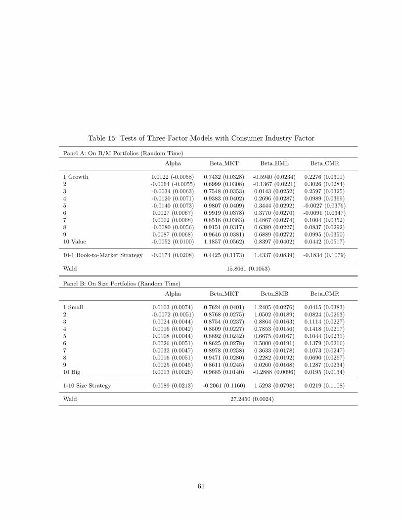
Table 15: Tests of Three-Factor Models with Consumer Industry Factor

Panel A: On B/M Portfolios (Random Time)

Alpha Beta MKT Beta HML Beta CMR

1 Growth 0.0122 (-0.0058) 0.7432 (0.0328) -0.5940 (0.0234) 0.2276 (0.0301)2 -0.0064 (-0.0055) 0.6999 (0.0308) -0.1367 (0.0221) 0.3026 (0.0284)3 -0.0034 (0.0063) 0.7548 (0.0353) 0.0143 (0.0252) 0.2597 (0.0325)4 -0.0120 (0.0071) 0.9383 (0.0402) 0.2696 (0.0287) 0.0989 (0.0369)5 -0.0140 (0.0073) 0.9807 (0.0409) 0.3444 (0.0292) -0.0027 (0.0376)6 0.0027 (0.0067) 0.9919 (0.0378) 0.3770 (0.0270) -0.0091 (0.0347)7 0.0002 (0.0068) 0.8518 (0.0383) 0.4867 (0.0274) 0.1004 (0.0352)8 -0.0080 (0.0056) 0.9151 (0.0317) 0.6389 (0.0227) 0.0837 (0.0292)9 0.0087 (0.0068) 0.9646 (0.0381) 0.6889 (0.0272) 0.0995 (0.0350)10 Value -0.0052 (0.0100) 1.1857 (0.0562) 0.8397 (0.0402) 0.0442 (0.0517)

10-1 Book-to-Market Strategy -0.0174 (0.0208) 0.4425 (0.1173) 1.4337 (0.0839) -0.1834 (0.1079)

Wald 15.8061 (0.1053)

Panel B: On Size Portfolios (Random Time)

Alpha Beta MKT Beta SMB Beta CMR

1 Small 0.0103 (0.0074) 0.7624 (0.0401) 1.2405 (0.0276) 0.0415 (0.0383)2 -0.0072 (0.0051) 0.8768 (0.0275) 1.0502 (0.0189) 0.0824 (0.0263)3 0.0024 (0.0044) 0.8754 (0.0237) 0.8864 (0.0163) 0.1114 (0.0227)4 0.0016 (0.0042) 0.8509 (0.0227) 0.7853 (0.0156) 0.1418 (0.0217)5 0.0108 (0.0044) 0.8892 (0.0242) 0.6675 (0.0167) 0.1044 (0.0231)6 0.0026 (0.0051) 0.8625 (0.0278) 0.5000 (0.0191) 0.1379 (0.0266)7 0.0032 (0.0047) 0.8978 (0.0258) 0.3633 (0.0178) 0.1073 (0.0247)8 0.0016 (0.0051) 0.9471 (0.0280) 0.2282 (0.0192) 0.0690 (0.0267)9 0.0025 (0.0045) 0.8611 (0.0245) 0.0260 (0.0168) 0.1287 (0.0234)10 Big 0.0013 (0.0026) 0.9685 (0.0140) -0.2888 (0.0096) 0.0195 (0.0134)

1-10 Size Strategy 0.0089 (0.0213) -0.2061 (0.1160) 1.5293 (0.0798) 0.0219 (0.1108)

Wald 27.2450 (0.0024)

61

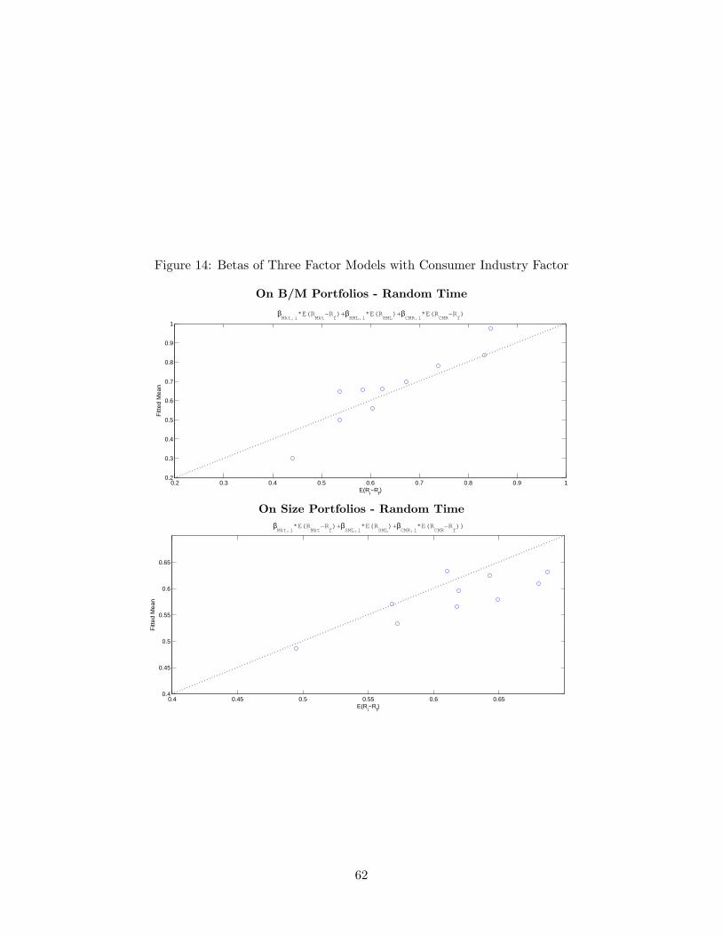
Figure 14: Betas of Three Factor Models with Consumer Industry Factor

On B/M Portfolios - Random Time

0.2 0.3 0.4 0.5 0.6 0.7 0.8 0.9 10.2

0.3

0.4

0.5

0.6

0.7

0.8

0.9

1

βMkt,i

*E(RMkt

−Rf)+ β

HML,i*E(R

HML)+ β

CMR,i*E(R

CMR−R

f)

E(Ri−R

f)

Fitt

ed M

ean

On Size Portfolios - Random Time

0.4 0.45 0.5 0.55 0.6 0.650.4

0.45

0.5

0.55

0.6

0.65

βMkt,i

*E(RMkt

−Rf)+ β

SML,i*E(R

SML)+ β

CMR,i*E(R

CMR−R

f))

E(Ri−R

f)

Fitt

ed M

ean

62

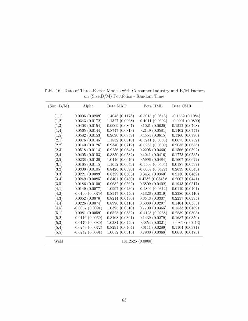
Table 16: Tests of Three-Factor Models with Consumer Industry and B/M Factorson (Size,B/M) Portfolios - Random Time

(Size, B/M) Alpha Beta MKT Beta HML Beta CMR

(1,1) 0.0005 (0.0209) 1.4048 (0.1178) -0.5015 (0.0843) -0.1552 (0.1084)(1,2) 0.0343 (0.0172) 1.1327 (0.0968) -0.1011 (0.0692) -0.0001 (0.0890)(1,3) 0.0408 (0.0154) 0.9009 (0.0867) 0.1021 (0.0620) 0.1522 (0.0798)(1,4) 0.0565 (0.0144) 0.8747 (0.0813) 0.2149 (0.0581) 0.1402 (0.0747)(1,5) 0.0582 (0.0153) 0.9690 (0.0859) 0.4554 (0.0615) 0.1360 (0.0790)(2,1) 0.0076 (0.0145) 1.1832 (0.0818) -0.5241 (0.0585) 0.0675 (0.0752)(2,2) 0.0140 (0.0126) 0.9340 (0.0712) -0.0265 (0.0509) 0.2038 (0.0655)(2,3) 0.0518 (0.0114) 0.9256 (0.0643) 0.2295 (0.0460) 0.1566 (0.0592)(2,4) 0.0405 (0.0103) 0.8850 (0.0582) 0.4041 (0.0416) 0.1773 (0.0535)(2,5) 0.0238 (0.0120) 1.0446 (0.0676) 0.5996 (0.0484) 0.1607 (0.0622)(3,1) 0.0165 (0.0115) 1.1652 (0.0649) -0.5566 (0.0464) 0.0187 (0.0597)(3,2) 0.0300 (0.0105) 0.8426 (0.0590) -0.0008 (0.0422) 0.2639 (0.0543)(3,3) 0.0221 (0.0089) 0.8329 (0.0503) 0.3451 (0.0360) 0.2130 (0.0462)(3,4) 0.0249 (0.0085) 0.8401 (0.0480) 0.4732 (0.0343)‘ 0.2007 (0.0441)(3,5) 0.0186 (0.0100) 0.9682 (0.0562) 0.6809 (0.0402) 0.1943 (0.0517)(4,1) 0.0149 (0.0077) 1.0997 (0.0436) -0.4860 (0.0312) 0.0119 (0.0401)(4,2) -0.0160 (0.0079) 0.8547 (0.0446) 0.1326 (0.0319) 0.2386 (0.0410)(4,3) 0.0052 (0.0076) 0.8214 (0.0430) 0.3543 (0.0307) 0.2237 (0.0395)(4,4) 0.0226 (0.0074) 0.8996 (0.0416) 0.5080 (0.0297) 0.1404 (0.0383)(4,5) -0.0057 (0.0091) 1.0395 (0.0510) 0.7700 (0.0365) 0.1533 (0.0469)(5,1) 0.0081 (0.0059) 0.6528 (0.0332) -0.4128 (0.0238) 0.2839 (0.0305)(5,2) -0.0116 (0.0069) 0.8168 (0.0391) 0.1439 (0.0279) 0.1687 (0.0359)(5,3) -0.0170 (0.0080) 1.0384 (0.0449) 0.3854 (0.0321) -0.0860 (0.0413)(5,4) -0.0259 (0.0072) 0.8291 (0.0404) 0.6111 (0.0289) 0.1104 (0.0371)(5,5) -0.0242 (0.0091) 1.0052 (0.0515) 0.7930 (0.0368) 0.0650 (0.0473)

Wald 181.2525 (0.0000)

63

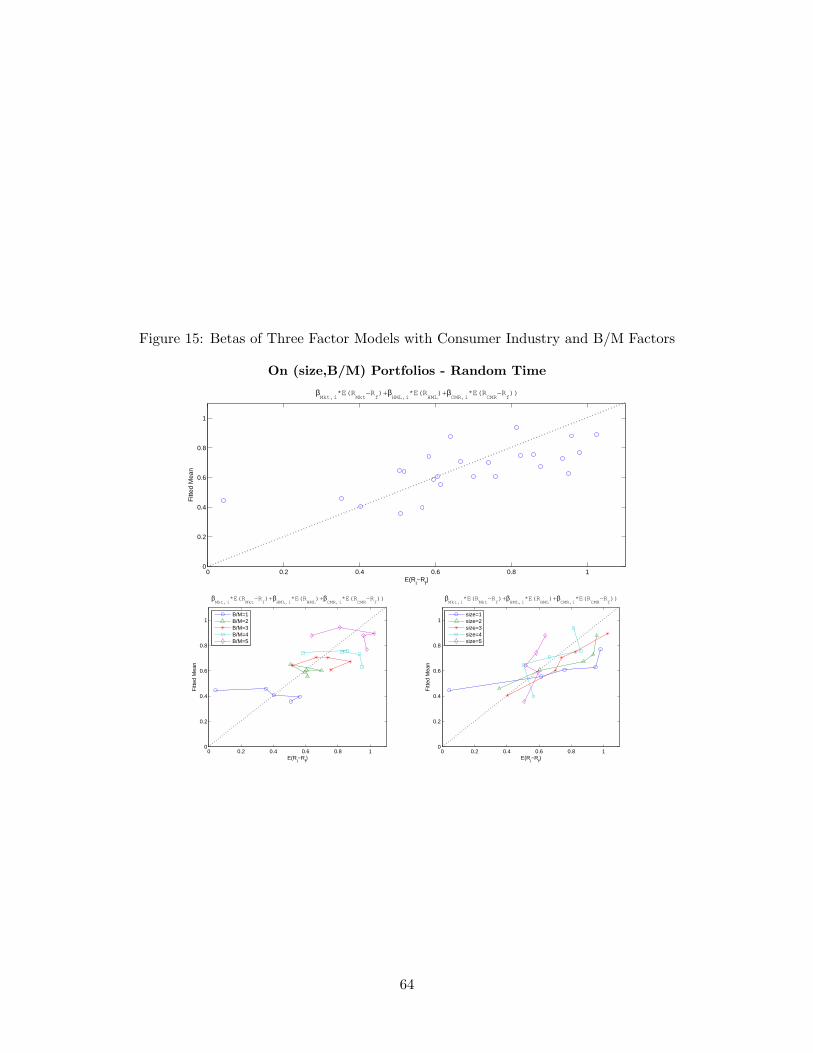
Figure 15: Betas of Three Factor Models with Consumer Industry and B/M Factors

On (size,B/M) Portfolios - Random Time

0 0.2 0.4 0.6 0.8 10

0.2

0.4

0.6

0.8

1

βMkt,i

*E(RMkt

−Rf)+ β

HML,i*E(R

HML)+ β

CMR,i*E(R

CMR−R

f))

E(Ri−R

f)

Fitt

ed M

ean

0 0.2 0.4 0.6 0.8 10

0.2

0.4

0.6

0.8

1

βMkt,i

*E(RMkt

−Rf)+ β

HML,i*E(R

HML)+ β

CMR,i*E(R

CMR−R

f))

E(Ri−R

f)

Fitt

ed M

ean

B/M=1B/M=2B/M=3B/M=4B/M=5

0 0.2 0.4 0.6 0.8 10

0.2

0.4

0.6

0.8

1

βMkt,i

*E(RMkt

−Rf)+ β

HML,i*E(R

HML)+ β

CMR,i*E(R

CMR−R

f))

E(Ri−R

f)

Fitt

ed M

ean

size=1size=2size=3size=4size=5

64