a conditional logit approach to u.s. state-to...

A CONDITIONAL LOGIT APPROACH TO U.S. STATE-TO-STATEMIGRATION*

Paul S. DaviesOffice of Research, Evaluation, and Statistics, Social Security Administration, 500 EStreet SW, 9th Floor, Washington, DC 20254, U.S.A. E-mail: [email protected]

Michael J. GreenwoodDepartment of Economics, University of Colorado, Boulder, CO 80309, U.S.A. E-mail:[email protected]

Haizheng LiSchool of Economics, Georgia Institute of Technology, Atlanta, GA 30332, U.S.A. E-mail:[email protected]

ABSTRACT. This paper uses a conditional logit approach to study interstate migrationin the United States for each of eleven years, from 1986–1987 to 1996–1997. We testsubstantive hypotheses regarding migration in the United States and demonstrate therichness of the conditional logit approach in studies of place-to-place migration. Weinvestigate migration responses to relative economic opportunities (unemployment rate,per capita income) and the associated costs of moving (distance between origin anddestination and its square). We also investigate how noneconomic factors, such as ameni-ties, affect migration between states through a state fixed effect. Finally, we study themagnitude of unmeasured costs associated with a particular migration. The conditionallogit model also allows us to compute various trade-off and other values that are of interestin migration analysis.

1. INTRODUCTION

Early models of the determinants of migration used aggregate data andemphasized place characteristics (Greenwood, 1975). Individual characteristicslike age and education were sometimes crudely proxied by variables relating tothe (origin) population at risk to migrate, but variables relating to personalcharacteristics were frequently lacking significance or were of unanticipatedsign. Such findings were hardly surprising because the aggregate variables were

© Blackwell Publishers 2001.Blackwell Publishers, 350 Main Street, Malden, MA 02148, USA and 108 Cowley Road, Oxford, OX4 1JF, UK.

*The views and interpretations expressed in this paper are the authors’ only and do not reflectthe official position of the Social Security Administration or any other federal agency. We are gratefulto Richard Cebula, the late Steven Sandell, seminar participants at the Georgia Institute ofTechnology, and especially three anonymous referees for helpful comments.

Received

337

JOURNAL OF REGIONAL SCIENCE, VOL. 41, NO. 2, 2001, pp. 337–360

often virtually uncorrelated with the migrant traits of concern (Navratil andDoyle, 1977).

During more recent years, with the availability of various microdata sets,discrete-choice models of the decision to migrate have become fairly standard.For example, logit and probit models have greatly enhanced the understandingof the underlying determinants of the decision to migrate.Early versions of thesemodels tended to include only personal characteristics (Linneman and Graves,1983), but later versions incorporated both personal and place characteristics(Herzog and Schlottmann, 1986).

In the context of models based on aggregate data, as well as many modelsbased on microdata, one of the most troubling problems is the treatment ofalternative destinations. Whereas various investigators address this problem,until recently none of them account for opportunities at all alternative destina-tions. They consider only a single alternative destination, such as that with thebest alternative income or the lowest alternative unemployment rate (Wadycki,1974). In some cases when alternative destinations are taken into account,staying at the present location is not in the choice set (Blank,1988; Bartel, 1989).This approach is often rationalized as a decision maker first deciding whetherto move, and given a decision to move, then deciding where to move. However,the decision regarding whether to move cannot reasonably be separated fromthe decision regarding where to move. Presumably, the decision to stay or go isbased on a rational consideration of the alternatives relative to the presentlocation.

A better method of approaching this problem is in the context of a condi-tional logit model in which the decision to stay is one option, along with aconsideration of all potential alternative destinations. The most importantdistinction between the conditional logit model and the approach used in earlystudies based on aggregate data is that the former has a sound microeconomicfoundation. The conditional logit model is built on an individual utility maximi-zation framework that is based on a random utility model. This is the method-ology adopted in the present study. We use aggregate state-to-state migrationflow data in the context of an individual random-utility-based conditional logitmodel to examine migration choices. In particular, each state (including thecurrent state of residence) is treated as a potential destination choice. Based onutility maximization, individuals may choose to migrate to any state or to stayin the current state. Given that we observe how many individuals move betweeneach pair of states, we develop a maximum likelihood function for estimationbased on the conditional logit model.

Earlier models of state-to-state migration focused on migration over agiven time interval. For example, models estimated with Census data typi-cally analyze migration over five year intervals (e.g., between 1985 and 1990).Although some data sets have the potential to yield annual logit or probitestimates of the determinants of migration, they have not been used in this way.Thus, migration researchers have little information about the repre-sentativeness of their parameter estimates over time. In this paper, we estimate

© Blackwell Publishers 2001.

338 JOURNAL OF REGIONAL SCIENCE, VOL. 41, NO. 2, 2001

our conditional logit model for eleven consecutive years (1986–1987 through1996–1997) using repeated cross-sections of the Area-to-Area Migration FlowData from the Internal Revenue Service. Although they are not panel databecause we cannot follow specific individuals in different years, these data stillprovide us with some sense of the temporal pattern and stability of our parame-ter estimates. Furthermore, annual estimation imposes few restrictions on themodel because all parameters are allowed to vary across time. This procedureis less restrictive than pooling data from multiple cross-sections and using timedummies to partially control for time trends.

Another way that the present study differs from earlier studies is in ourtreatment of the distance variable. In logit or probit models of the decision tomigrate, a distance variable has no place because no specific destination isidentified. However, in the conditional logit model developed here, variousdestinations are specified and thus distance has a role to play. In most earlierstudies that include a distance variable, the implicit assumption is that therelationship between distance and migration is linear or linear in logarithms.However, the deterring effects of distance may decline at greater distancesbecause the marginal cost of moving a unit distance farther is lower at greaterdistances. Thus, we include distance squared in the model.

Finally, we use our conditional logit approach to examine trade-offs relatedto the probability of migration for certain pairs of variables. By measuring thetrade-off between a given variable and per capita income, we can place a roughdollar value on that trade-off. One such trade-off, that between distance anddestination income, was noted by Sjaastad (1962, p.84).

Ideally, to study migration behavior both choice attributes and individualcharacteristics will be included in the model. However, with a large number ofpotential destination choices (states), the computation cost for this maximumlikelihood estimation is very high. Therefore, we impose some additional restric-tions on the model. First, the conditional logit model focuses on the effect ofchoice-specific attributes on the migration decision to identify how the charac-teristics of a state affect an individual’s destination choice. The parameters areassumed to be constant across choices. The effects of individual characteristicsgenerally cannot be directly identified with the conditional logit model. Theconditional logit model is different from the multinomial logit model of migrationthat focuses on the effects of individual characteristics on the migration decision.For a multinomial logit model, the corresponding parameters are different fordifferent choices (Schmidt and Strauss, 1975). However, it is difficult to incorpo-rate this degree of flexibility when studying state-to-state migration. There areup to fifty potential destination choices so the number of parameters quicklybecomes too large for computation. Moreover, we do not have data on individualcharacteristics such as age and education.

Second, an individual’s migration choice should be based on comparisons ofthe characteristics of possible destinations with those of the current state ofresidence. Therefore, the characteristics of the current state of residence can bethought of as a kind of individual characteristic. That is, a characteristic in a


DAVIES, GREENWOOD, & LI: STATE-TO-STATE MIGRATION 339

destination state will be viewed differently for individuals in different origins.In the conditional logit model the effects of individual characteristics cannot bedirectly identified, so we incorporate these origin characteristics by usingrelative measures of attributes between potential destinations and the origin.Although this specification is somewhat restrictive, the use of relative measuresis appealing in the sense that it captures the notion that the migration choiceis based on comparisons of potential destinations with the origin.

Third, an important aspect of our model specification is that we include aset of choice dummy variables (state fixed effects). This greatly increases thenumber of parameters and causes convergence problems. To reduce the numberof parameters, we combine some states and specify state-group fixed effects.Finally, the Independence of Irrelevant Alternatives (IIA) property is requiredfor the conditional logit model. We conduct only limited tests of this property,but the tests cannot reject the validity of the IIA property.

Although these restrictions should be kept in mind in interpreting theresults, our estimation results are consistent and robust across years. Fur-thermore, this study demonstrates that the conditional logit approach canprovide a variety of results and is a powerful tool in studying migration.Results from alternative specifications are reported also. Although we do notinclude personal characteristics such as age and education in the model, thisdoes not change the fact that the model is based on individual behavior. Eachindividual’s choice is based on utility maximization, and the probability of aparticular choice for an individual enters the likelihood function inde-pendently. The likelihood function is constructed from the observed choices(migration) of the entire sample. In addition, individuals who move to thesame destination state but from different origins are treated differentlybecause the attributes of the origin states differ.

The rest of this paper proceeds as follows.Section 2 presents the econometricmodel and discusses some limitations of the approach. Section 3 describes thedata. Section 4 discusses the results. Finally, section 5 provides a brief summaryand conclusions.

2. ECONOMETRIC MODEL

The conditional logit model for migration choices is motivated by a randomutility model. An individual at area i faces J choices, including moving to adifferent area or staying at the current location. Suppose that the utility levelof choosing area j for this individual is

Uij = β′Xij + εij

where Xij is a vector of choice-specific attributes. For the conditional logit, theparameter β is constant across choices. If the individual chooses destination j,then the utility Uij is the highest among all J choices (i.e., Uij >Uik for all k ≠ j).Thus, when choice j is made, the statistical model for the probability of movingfrom area i to area j can be represented as



P(yi = j) = P(Uij > Uik) ∀ k ≠ j

Based on McFadden (1973), if and only if the J disturbances are independentand identically distributed with the Weibull distribution, then the probability ofan individual at area i choosing area j (where j = i for nonmovers) is

The log likelihood function for all individuals moving from any area i to aspecific area j is

where mij = 1 if an individual in area i chooses destination area j.In this framework, if individuals do not move they choose to remain in

the current location. This is an important aspect of our model because itallows us to estimate the unobserved difference between moving and staying.One alternative to this specification is to eliminate the current area ofresidence from the choice set and to focus on movers only. This specificationwould cause a selectivity problem because the possibility of a stayer movingunder certain conditions is eliminated. Another specification is based on thenested logit model (McFadden 1984, Maddala 1983) where a person’s migra-tion is treated as two separate decision procedures: first, the decision to moveor to stay; second, given the decision to move, the choice of a destination. Thisnested approach is not adopted in this study because we believe that thedecision to migrate and the choice of a destination are unlikely to be madesequentially. Rather, the decision regarding whether to move is intimatelyrelated to the possible destination choices.

We focus on migration between states in the coterminous U.S. Individualswho work in Washington, DC may reside in Maryland or Virginia so thesethree areas are combined into one destination choice. Thus, we have a totalof 47 potential destination choices (including the current state of residence)for each individual. We have 47 source states because for each destinationpeople can migrate from any other state. The corresponding log-likelihoodfunction is

where Nij is the number of people moving from state i to state j and

P y je

ei

x

x

k

ij

jk= =

′

′∑b g

β

β

ln lnL m P mij iji

= =∑ 1d i

ln lnL N P mijji

ij= ===

∑∑1

47

1

47

1d i



is the probability of moving from state i to state j.1

The xij vector includes choice-specific attributes such as economic factorsthat will affect individuals’ migration choices. Clearly, unobservable economicand noneconomic state characteristics such as amenities (Greenwood et al.,1991) also play an important role in the migration decision. To capture theseeffects we include a set of dummy variables for potential destinations (state fixedeffects). These choice dummy variables are important for the specification of theconditional logit model because they function as constant terms (the inclusionof a separate constant term will drop out of the probability function).

Another consideration is the choice of the current state if an individualchooses not to move. A substantial difference should exist between this choice(the current state) and all other choices (another state) because no migrationoccurs if the current state is chosen. The difference between moving and stayingcannot be controlled by state fixed effects alone because it also is related tounobserved costs associated with moving. To control for these unobservedfactors, we include a nonmigration dummy variable in the model that is equalto one if the current state of residence is chosen and zero otherwise.

In the conditional logit model, only the effects of choice-specific attributescan be identified. A migration decision is based on the comparison of destinationstate characteristics with the characteristics of the current state of residence,so source state characteristics will certainly affect the migration choice. Forexample, people in a high-income source state i will view the income level in apotential destination state k differently than people in a low-income source statej. However, because source state characteristics do not vary across choices foran individual, they will drop out of the probability function.

Several options are available for treating this problem. The first is to useonly the characteristics of a potential destination state, ignoring those of thesource state. This option is clearly very restrictive. The second option is to

P me

eij

x

x

k

ij

ik

= =′

′

=∑

1

1

47d iβ

β

1As pointed out by an anonymous referee, an alternative specification of the model wouldexplicitly control for the quantity of opportunities available at the destination on the grounds thatthe probability of choosing destination state j should be linearly homogeneous in the number ofalternatives available in state j (Ben-Akiva and Watanatada, 1981). Imposing linear homogeneity,the probability function is specified as

where y is a proxy for the quantity of opportunities avaliable at the destination. Results from thisspecification are discussed below.

P my e

y eij

jx

kx

k

ij

ik

= =′

′

=∑

1

1

47d iβ

β



interact origin state variables with the destination choice dummy variables(state fixed effects).However, this procedure increases the number of parametersdramatically due to the large number of destination choice dummies. In fact, ifall variables for an origin state are interacted with all destination choicedummies, the conditional logit model becomes the multinomial logit modelbecause the parameters effectively vary across choices. The third option is to userelative measures of variables for the destination and origin by creating explana-tory variables that take the form of destination-to-origin ratios. The further thevalue of the ratio from one, the larger the relative difference between thedestination and the origin, and thus, the larger the influence of the variable onthe probability of moving. This approach is restrictive because it essentiallyrequires symmetric responses for changes in an origin state and a destinationstate characteristic.

Among these options, the second appears to be the best. However, perhapsdue to the large number of parameters, the likely correlation between thedestination characteristics and the state fixed effects, and large scalingdifferences between the independent variables, it fails to converge in compu-tation. We adopt the third option and use ratio measures of destination andorigin characteristics in our estimation to avoid computation problems. Moreimportantly, we feel that ratio measures of the independent variables arebetter suited to capture the likely influence of differences between destina-tion and origin characteristics on migration choice. We test the sensitivity ofour specification by running alternative specifications using only destinationcharacteristics. In our preferred specification, the destination choice dummyvariables are replaced by 26 state-group dummies, where states are groupedbased on similarity in terms of geography and amenities. As a result, thecoefficients on the variables representing location characteristics (i.e., popu-lation, unemployment rate, and per capita income) are largely identified bydifferences within the state groups. This approach is justified because thestate groupings result in sets of states that are likely to be similar withrespect to unmeasured characteristics.

Finally, the conditional logit model depends on the independence ofirrelevant alternatives (IIA) assumption. That is, the relative probabilitiesbetween choices must be independent of other alternatives. The IIA assump-tion follows from the initial assumption that the disturbances are inde-pendent and homoskedastic for the random utility model. Two types of testsare available for the IIA assumption, a Hausman-type specification test(Hausman and McFadden, 1984) and a Lagrange multiplier test (McFadden,1987). These tests can be conducted by eliminating a subset of the choicesfrom the choice set and reestimating the model. If the parameters of therestricted model are not systematically different from the parameters of thefull model, then the IIA property holds. In this study with 47 potential



destination choices, the number of subset combinations to test is enormous.2

Furthermore, these tests do not offer a guideline for selecting the subset ofstates to eliminate.

Nevertheless, we conduct limited tests of the IIA property by first eliminat-ing Florida from the choice set and then eliminating Colorado. Although thechoice of these states is somewhat arbitrary, both states are similar in terms oftheir importance as receiving states of internal migrants, whereas they differgreatly in many other respects. The IIA test is conducted following Hausmanand McFadden (1984). The test statistic is

χ2 = (bs – bf)′ (Vs –Vf)–1 (bs – bf)

It has the χ2 distribution with k degrees of freedom, where k is the rank of(Vs –Vf). The parameter estimates based on the restricted subset of states andthe full subset of states are bs and bf, respectively. Vs and Vf are the respectiveestimates of the asymptotic covariance matrices.

In both tests, k is equal to 31. (The state dummy variable that cannot beidentified in the restricted choice set also is removed from the full parametervector.) The corresponding χ2 test statistic is 1.13 when Florida is eliminatedand 0.11 when Colorado is eliminated. The critical value for the χ2 statistic with31 degrees of freedom at the 10 percent level is 41.33. Clearly, in both cases, wecannot reject the hypothesis that the IIA property holds for the choice set.Although the IIA test generally has low power, these limited results do not offerevidence against the conditional logit approach.

3. DATA AND EXPLANATORY VARIABLES

The migration data used in this paper are the Internal Revenue Service(IRS) Area-to-Area Migration Flow Data (hereafter referred to as “the IRSdata”). The IRS data provide a 51 × 51 matrix of internal migration flows for all50 states and the District of Colombia annually beginning in 1975–1976.Nonmovers are on the diagonal of the matrix. Our data cover the eleven-yearperiod from 1986–1987 through 1996–1997. We focus attention on moves withinthe coterminous United States and collapse Maryland, Virginia, and the Districtof Colombia into a single location. This leaves us with a 47 × 47 matrix ofstate-to-state migration flows and nonmovers.

Although this is a rich source of temporal state-to-state migration data,some limitations should be noted. The flows are calculated by matching SocialSecurity numbers from individual income tax returns and comparing addressesacross years. Approximately 94 percent of the population is covered, but treat-ment of spouses and dependents in households is unclear. Migration in the IRSdata is based on the Social Security number of the primary tax payer, so spouses

2For example, if we choose a single state as the subset, there are 47 different combinations(C) to test. If we choose two states as the subset, there are combinations to test.C47

2



and dependents may not get counted as either migrants or nonmigrants.Furthermore, individuals who leave a household and move during the same taxyear (e.g., divorce and move) may not be properly counted as movers. The extentof these problems is largely unknown. Finally, personal and household charac-teristics are not reported due to privacy and confidentiality restrictions. Thesepotential problems notwithstanding, the IRS data hold great potential fortemporal analyses of state-to-state migration.

Based on the discussion in the previous section,we include state fixed effectsand a nonmigration dummy variable in our specification. In addition, statepopulation is included as a comprehensive measure of the quality and quantityof all opportunities and social or family connections that are important tomigration. The population variable is constructed as the ratio of destination-to-origin state population. A large state has more locations from which to choose,as well as more connections, more opportunities, and more widely availableinformation that may serve to reduce the search costs and psychological costsassociated with migration. Therefore, population is a reasonable proxy for thenumber of locations and opportunities available at potential destinations. Otherproxies such as population density are used in alternative specifications.

State per capita income is included to represent the potential economicgains or losses from migration. It is measured as the ratio of destination-to-origin per capita income. The hypothesis that we test is that migrants areattracted to destinations with relatively higher per capita incomes. The ratio ofdestination-to-origin state unemployment rates is included as a comparison ofdifferent job opportunities (or the lack of job opportunities) between destinationand origin states. The hypothesis here is that relatively higher destinationunemployment rates deter migration. Distance, measured in thousands of milesbetween states, is used as a proxy for the direct economic costs and indirectpsychological costs related to migration. Distance squared is included to accountfor nonlinear effects associated with increased distance.

The independent variables are derived from various sources. Per capitaincome and population are from the Regional Economic Information Systems(REIS) data file for 1986–1991 and from the Statistical Abstract of the UnitedStates: 1998 for 1992–1996.3 Distances between states are from Rand-McNally’s Highway Mileage Guide and represent highway mileages betweenprincipal cities in each state. The unemployment rate for each state is fromthe Bureau of Labor Statistics’ Monthly Labor Review for 1986–1991 and fromthe Bureau of Labor Statistics’ Local Area Unemployment Statistics for1992–1996. For Maryland, Virginia, and the District of Colombia as a singlelocation, per-capita income and the unemployment rate are calculated as

3Ideally, per capita income is adjusted for state cost-of-living differences. McMahon (1991)computes state cost-of-living indices; however, they do not cover the entire period of our data. Evenif we were to adjust for interstate differences in cost-of-living, intrastate differences in cost-of-livingwould still remain.



weighted averages. Distance from the Maryland-Virginia-District of Colombialocation is measured from the District of Colombia.

Initially, we created one dummy variable for each state, resulting in46 dummy variables and a total of 52 parameters to be estimated. The compu-tation failed to converge, perhaps due to the large number of parameters to beestimated and the likely correlation between the state fixed effects and thedestination characteristics. To reduce the number of parameters, we combine“similar” states for the state dummy variables, based on similarity in terms ofgeographic location and amenities. This specification may also help to reducethe correlation between the individual state dummy variables and the destina-tion characteristics. A total of 26 state-group dummies are created with Califor-nia as the omitted choice (see Table A1 for the state-group combinations).

After incorporating these variables, the probability function for an individ-ual at state i to move to state j is (for simplicity, we drop the origin notation i)

where = (xj1, xj2, xj3) = destination-to-origin population ratio, destination-to-origin unemployment rate ratio, and destination-to-origin per capita income ratio,respectively; = (z1, z2, . . ., z26) = state-group dummy variables; wj = distance(thousands of miles) between i and j; and s = the nonmigration dummy variable.

4. RESULTS

The conditional logit model described above is estimated separately for eachof eleven years, 1986–1987 through 1996–1997.4 Estimated coefficients for theprimary explanatory variables for each year are presented in Table 1. A numberof alternative specifications also are estimated.5 The results from some of thesealternative specifications are presented in Table A2.6

Pe

ej

x z w w s

x z w w s

j

j j j j

j j j j

=′ + ′ + + +

′ + ′ + + +

=∑

β α γ θ δ

β α γ θ δ

2

2

1

47

′x j

′z j

4The computer software package used is GAUSS. It takes 1 to 5 hours for convergence foreach year, depending on the starting values, on a Pentium II 300 processor.

5The destination-to-origin population ratio is included in the vector of choice-specific attrib-utes to control for the quality and quantity of opportunities offered at the destination relative to theopportunities available at the origin. In one alternative specification, we impose linear homogeneity(as described in footnote 1) using destination state population as a proxy for the quantity ofopportunities available at the destination. The results, (available from the authors on request) arevery similar to the results of our original specification (Table 1) in all respects (sign, magnitude, andsignificance). Given this and noting that the specification imposing linear homogeneity is morerestrictive, we prefer the original specification.

6The results from the alternative specifications in Table A2 and are very similar to the resultspresented in Table 1. One difference is that the coefficient for population density in column 1 isnegative and significant, whereas the coefficient of the population ratio variable is always positiveand significant.We believe that although greater population density may represent greater potentialopportunities, it also may represent greater congestion, thus leading to the negative coefficient.



TABLE 1: Estimated Coefficients from Conditional Logit, Primary Explanatory Variables, 1986–1996a

Variable 1986 1987 1988 1989 1990 1991 1992 1993 1994 1995 1996

Populationb 0.036 0.033 0.038 0.032 0.031 0.031 0.032 0.032 0.031 0.029 0.031(0.0022) (0.0006) (0.0022) (0.0013) (0.0017) (0.0001) (0.0059) (0.0039) (0.0043) (0.0037) (0.0026)

Unemployment Rateb –0.78 –0.66 –0.73 –0.41 –0.74 –0.22 –0.44 –0.48 –0.38 –0.30 –0.58(0.0008) (0.0008) (0.0011) (0.0023) (0.0014) (0.0010) (0.0028) (0.0004) (0.0002) (0.0020) (0.0073)

Per Capita Incomeb 0.81 0.81 0.59 0.71 0.38 0.79 0.58 0.51 0.81 1.00 0.76(0.0029) (0.0013) (0.0011) (0.0009) (0.0040) (0.0003) (0.0007) (0.0008) (0.0002) (0.0018) (0.0013)

Distance –1.72 –1.72 –1.68 –1.73 –1.72 –1.74 –1.69 –1.74 –1.74 –1.78 –1.82(0.0020) (0.0014) (0.0006) (0.0013) (0.0007) (0.0001) (0.0020) (0.0015) (0.0002) (0.0004) (0.0005)

Distance Squared 0.41 0.41 0.40 0.41 0.40 0.41 0.39 0.40 0.40 0.42 0.43(0.0002) (0.0011) (0.0003) (0.0006) (0.0003) (0.0005) (0.0004) (0.0005) (0.0008) (0.0002) (0.0004)

Non-Migration Dummy 6.09 6.11 6.11 6.11 6.10 6.17 6.17 6.15 6.13 6.14 6.12(0.0007) (0.0007) (0.0003) (0.0004) (0.0004) (0.0001) (0.0010) (0.0011) (0.0002) (0.0013) (0.0006)

log L at Convergencec –4.39 –4.26 –4.31 –4.47 –4.25 –4.21 –4.29 –4.29 –4.37 –4.29 –4.35log L at β = 0c –75.2 –74.1 –75.4 –77.5 –74 –77.4 –77.7 –77.9 –77.9 –78.8 –79.9log L at Sample Sharesc –67.2 –66.2 –67.3 –69.1 –66 –68.9 –69.3 –69.5 –69.6 –70.5 –71.5

aAll estimated coefficients are statistically significant at the one percent level. Standard errors are in parentheses.bDestination-to-origin ratiocAll log L values are divided by ten million.

©B

lackwellP

ublishers

2001.

DA

VIE

S,GR

EE

NW

OO

D,&

LI:S

TA

TE

-TO

-ST

AT

EM

IGR

AT

ION

347

The results for most of the primary independent variables are strong andconsistent across time.The last three rows of Table 1 show that the log-likelihoodratio is much larger at convergence (log L at convergence) than when evaluatedwith all coefficients set to zero or at the sample shares of migration flows. Thisis a general indication that our model explains the data better than no model(β = 0) and better than a simple description of the data based on sample shares.7

For the conditional logit model, the direct marginal effects for continuousvariables are

and

The marginal effects of a one standard deviation change in the unemploymentrate ratio and the per capita income ratio for selected i-j pairs of states in 1996are discussed in the text below. Table 2 presents the marginal effect of a onehundred mile increase in distance between the origin and destination for thesame i-j pairs of states in 1996.8 The marginal effects are scaled by theprobability of moving from state i to state j, allowing the marginal effects to be

∂∂

βPx

P Pi

ii i= −1b g

∂∂

γ θPw

P P wi

ii i j= − +1 2b gd i

A migrant stock variable is sometimes included as an independent variable in models ofmigration (Greenwood, 1969) to proxy for the effect of having family and friends at the potentialdestination. The coefficient for migrant stock in column 4 is negative and significant, whereas weexpected it to be positive. To the extent that the previous year’s migration flow from state i to statej may not be stable (e.g., many of these migrants may move on to other destinations or may returnto the origin) and that new migrants may provide negative information to family and friends at theorigin (e.g., homesick, unhappy with new job or residence), it may not accurately reflect the familyand friends effect as in Greenwood (1969). Other constructions of migrant stock, such as the sum offlows from state i to state j over the previous five years, may suffer from even greater measurementerror because we cannot identify how many of these migrants stay in state j. As noted by ananonymous referee, our proxy for migrant ‘stock’ is actually a ‘flow’ measure.A better measure wouldcross-tabulate state of current residence by state of birth from decennial census data. However, atbest such a measure (from the 1990 census) would be applicable to our 1991 and 1992 migrationdata; Therefore, we do not follow this approach. As noted in Greenwood (1997), if migrant stock isnot included, the distance variable (and in this case, distance squared) reflects the importance ofrelatives and friends at the destination, as well as the direct economic costs of moving.

7On average, our model over-predicts out-migration. The maximum value of the predicted-to-actual out-migration ratio occurs for Maine and Vermont in each year. The minimum value occursfor Florida in each year.

8Four states, one from each Census region, are followed throughout the discussion of results.These states are Arizona, Illinois, Massachusetts, and Tennessee. These states were chosen arbitrar-ily apart from the desire to include one state from each Census region. Clearly, other states couldhave been chosen and would display somewhat different results.The results from 1996 are presentedbecause this is the most recent year of our data.



interpreted as proportional changes. Thus, the Pj term drops out of the equationsabove when considering proportional changes.

The result in Table 1 that migrants are more likely to move to relativelymore populous states may suggest that people move to places of greater per-ceived economic and social opportunity. To the extent that information is morewidely available about locations and potential opportunities in more populousstates, search costs and pshychological costs associated with migration may belower, thereby increasing the probability of migrating to a relatively morepopulous state. The results across years for population are very consistent—theestimated coefficient is between 0.029 and 0.038 for each of the eleven years ofour analysis.

In models of place-to-place migration, unemployment-rate variables consis-tently have had insignificant coefficients and unanticipated signs (Greenwood,1975, 1997). However, it is noteable that this is not the case in our conditionallogit model. Migrants are significantly less likely to move to a destination witha relatively higher unemployment rate. Table 1 shows that the direction andsignificance of this result is consistent across all eleven periods. We attributethis result to the inclusion of state-group dummies. As shown in column 6 ofTable A2, when state-group dummies are excluded, the only substantivechange in the results is that the coefficient on the unemployment rate ratiobecomes positive and significant. This finding suggests that unmeasured differ-ences between states are important and that including state-group dummieshelps to identify the parameters. Therefore, we prefer the specification inTable 1 to the specification without state dummies in column 6 of Table A2(in Appendix).

Although the sign and significance of the unemployment rate coefficient isconsistent over time, the magnitude of the coefficient varies considerably, callinginto question the temporal representativeness of previous estimates of therelationship between the unemployment rate and the probability of migrationbased on a single cross-section of data. The range of estimated coefficients forthe unemployment-rate ratio extends from –0.22 in 1991 to –0.78 in 1986(Table 1). This finding appears to be driven by state variations in unemploymentrates. For 1986, the year for which the unemployment-rate coefficient is largest

TABLE 2: Proportional Changes in the Probability of Moving from State i toState j Due to a One Hundred Mile Increase in Distance Between

Destination and Origin, 1996

Destination

Origin Arizona Illinois Massachusetts Tennessee

Arizona –0.02638 0.04573 –0.03560Illinois –0.02638 –0.09943 –0.14321Massachusetts 0.04572 –0.09938 –0.08683Tennessee –0.03560 –0.14314 –0.08685



in absolute value, the mean state unemployment rate is 7.0 percent with avariance of 4.8. For 1991, the year for which the unemployment-rate coefficientis smallest in absolute value, the mean and variance are 6.4 percent and 2.1,respectively.9 The lower variance of state unemployment rates may provide lessinformation for prospective migrants to use in making their location choices;hence, the absolute values of the estimated coefficients are smaller for thoseyears. In other words, for these years, the unemployment rate plays a lessimportant role in the prospective migrant’s decision-making process becausestate unemployment rates are more evenly distributed across the nation. Asevidence in favor of this hypothesis, we note that for the period 1986–1996, thecorrelation between the estimated coefficient on the unemployment-rate vari-able and the variance in state unemployment rates is –0.52 and is statisticallydifferent from zero at the 10 percent significance level.

For 1996, a one-standard deviation change in the destination-to-originunemployment rate ratio reduces the probability of migration by between18 percent and 20 percent, depending on the pair of states (results not shown).As an example, consider a one-standard deviation increase in the Arizona-Illinois destination-to-origin unemployment rate ratio (from 1.04 to 1.38) causedby an increase in the destination unemployment rate for Arizona (from 5.5 per-cent to 7.3 percent). The proportional effect of this change is a 19.43 percentreduction in the probability of migration from Illinois to Arizona. The propor-tional effect of a change in the unemployment rate ratio on the probability ofmigration is quite stable across pairs of states in 1996.

Relative per capita income has the expected positive sign and is highlysignificant for each year (Table 1), indicating that migrants are more likely tomove to destinations with relatively higher per capita incomes or greaterperceived economic opportunities.The estimated coefficient on per capita incomehas a mean of 0.71 and a standard deviation of 0.17 across the years of ouranalysis. The variation in the coefficient estimates over time is considerable butdoes not appear to follow a consistent pattern. For 1996, a one-standard devia-tion change in the destination-to-origin per capita income ratio increases theprobability of migration by between 16 percent and 17 percent, depending onthe pair of states (results not shown). For example, a one-standard deviationincrease in the Illinois-Massachusetts destination-to-origin per capita incomeratio (from 0.90 to 1.11) caused by an increase in destination per capita incomefor Illinois (from 26,855 dollars to 33,087 dollars) increases the probability ofmigration from Massachusetts to Illinois by 16.25 percent. As is the case withthe unemployment rate ratio, the proportional effect of a change in the per capitaincome ratio on the probability of migration is very stable across pairs of statesin 1996.

9Means and variances are calculated from state unemployment rates for the 47 units used inthe analysis—46 coterminous states plus a combined unit including the District of Colombia,Maryland, and Virginia.



Table 1 indicates that the effect of distance on the probability of movingfrom state i to state j is negative, highly significant, and very stable acrossthe eleven periods. The finding that greater distance between origin anddestination deters migration is consistent with previous research. However,we also include distance squared as an explanatory variable to explore thepossibility that the effect of distance on migration is not linear. The resultsin Table 1 indicate that the deterrent effect of distance on the probability ofmigration decreases as distance increases. That is, as distance between originand destination increases, the probability of migration decreases, but at adiminishing rate.

Proportional changes in the probability of migration resulting from aone hundred mile increase in distance between origin and destination arepresented for 1996 in Table 2. These effects vary widely across pairs of states,are predominantly negative as expected, and are quite large in some cases.10

Although a one hundred mile increase in distance between Illinois and Arizonareduces the probability of migration between the two states by only 2.6 percent,the same change in distance between Illinois and Tennessee leads to a 14.3percent decrease in the probability of migration.

The nonmigration dummy variable identifies the decision to stay in theorigin state as distinct from the decision to move. The nonmigration variableallows us to obtain some measure of the unobserved costs of moving fromstate i to state j. These unobserved costs of moving can be thought of aspsychic costs and time costs of moving. Psychic costs include leaving familyand friends, and concerns about adjusting to the surroundings in the newlocation. Time costs of moving include packing and unpacking. The estimatedcoefficient on the nonmigration variable is positive and highly significant forall eleven periods (Table 1). The magnitude of the coefficient is stable overtime, ranging between 6.09 and 6.17. Moreover, the magnitude of the nonmi-gration coefficient relative to the coefficients for the other primary explana-tory variables suggests that unobserved costs of moving are important in thedecision to stay or move.

To interpret the coefficient of the nonmigration dummy variable, supposethere exists a hypothetical state j that is exactly the same as state i (origin) inall respects, including observable characteristics, amenities, and even distance(i.e., wij = 0). That is, one can stay in origin i without moving, or one can “jump”to destination j in which all of the costs associated with migration mentionedabove will be incurred. Then, all measured factors are the same, and the onlydifference between choosing state i and state j is conceptual migration. In this

10The marginal (proportional) effects become positive only for distances greater than approxi-mately 2,500 miles. For 1996, only 2.88 percent of all moves involved state pairs that are more than2,500 miles apart. Furthermore, only 0.15 percent of the at risk population (i.e., movers plus stayers)made a move of greater than 2,500 miles. The effect for the tails of the distribution may not beproperly identified because such a small proportion of moves occurred between states more than2,500 miles apart.



situation, the percentage difference in the probability of moving or not movingis measured by

For example, for 1996, all unobservable costs associated with the migrationdecision make the probability of moving 99.8 percent lower than the probabilityof not moving.

The conditional logit model also allows for the calculation of cross-marginaleffects because we are able to specify numerous alternative destinations. Cross-marginal effects can be interpreted as the effect of a change in a charac-teristic of alternative destination k on the probability of moving from origin ito destination j. For continuous variables, the cross-marginal effects are

where Pj is the probability of moving from state i to state j and Pk

is the probability of moving from state i to state k. The magnitudes of thecross-marginal effects are very small, as expected. Such estimates may be usefulin the context of a specific application. We are unaware of any previous use ofthe conditional logit approach to estimate cross-marginal effects associated withmigration. Bartel (1989) uses the conditional logit approach to examine thelocation choices of immigrants to the United States, but does not explorecross-marginal effects.

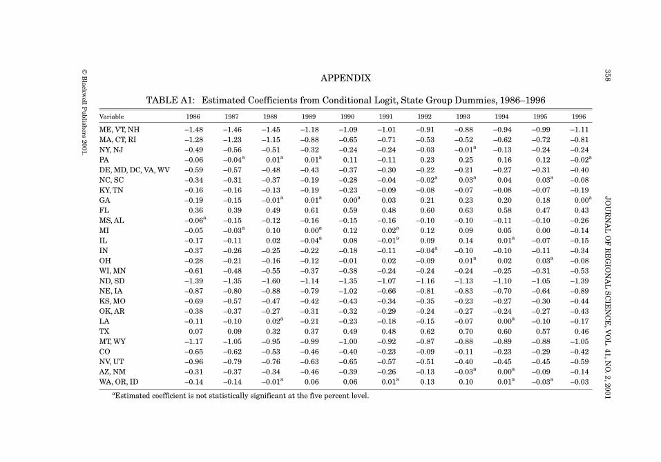
As described above, state-group fixed effects are included to capture unob-servable economic and noneconomic state factors associated with the migrationdecision, such as amenities. The vast majority of the estimated coefficients arestatistically significant (Table A1). The coefficients are predominantly negative,indicating that the state group is a relatively less attractive destination thanthe omitted choice, California. Texas and Florida, with consistently positiveestimated coefficients, appear to be relatively more attractive destinations thanCalifornia. The coefficients for Georgia are negative for the first few years andthen turn positive, indicating that Georgia’s attractiveness relative to Cali-fornia has changed over the period of our analysis. Still other states and stategroups, such as Illinois, Michigan, Ohio, North Carolina/South Carolina, andWashington/Oregon/Idaho, have coefficients that change sign more than oncebetween 1986 and 1996. This temporal pattern suggests that the attractivenessof these state-group destinations relative to California is fluctuating throughthe late 1980s and 1990s. Further research on the temporal patterns of thestate-group fixed effects could make useful contributions to the literature on therelative effects of amenities and other unobservable factors on the migrationdecision.

For certain pairs of independent variables, examination of trade-offsrelated to the probability of migration is of interest. We noted above thatSjaastad (1962) calculated the trade-off between distance and destination

P moving P not movingP not moving

eb g b g

b g− −

−= −−δ 1

∂∂

βP

xP Pj

kj k= −



income. The conditional logit approach allows us to calculate not only thistrade-off, but others as well. By measuring the trade-off between any givenvariable and per capita income, we can place an approximate dollar value onthat trade-off. Three trade-offs are derived and discussed below: the trade-offbetween the unemployment rate and per capita income, the trade-off betweendistance and per capita income, and a money measure of unobserved costsassociated with migration.11

If everything else is held constant, and only the unemployment-rate ratioand the per capita income ratio are allowed to change, then we can derive aniso-probability curve in unemployment-income space.12 The probability ofmoving from state i to state j is held constant (dPj = 0) and

For example, in 1996, this ratio is 0.76, which means that if the ratio of theunemployment rate between destination j and origin i increases by one, thecorresponding ratio of per capita income should increase by 0.76 to keep theprobability of moving constant. That is, if initially the unemployment rate inboth the origin and destination is 4 percent, but now the destination unemploy-ment rate increases to 8 percent, the per capita income ratio should increase by0.76 to compensate. If per capita income in both states is $10,000 initially, thendestination per capita income must increase by $7,600 to $17,600 to compensate.

Table 3 shows the increase in destination per capita income required to keepthe probability of moving constant, resulting from a one-standard deviationincrease in the unemployment-rate ratio and holding origin unemployment rateand per capita income constant.Among the four selected origin states, this dollaramount ranges from $5,428 for Arizona to $7,584 for Massachusetts. Some ofthe variation across states is likely due to state cost-of-living differences. Themagnitude of the unemployment rate–per capita income trade-off varies sub-stantially over the time period of our analysis as a result of changes in therelevant coefficients (per capita income also varies over time).

Following the same procedure but for distance and per capita income, weobtain

dx

dx

P

dx

P

dxj

j

j

j

j

j

3

2 2 3

2

3= = −

∂ ∂ ββ

dx

dw

P

w

P

x

wj

j

j

j

j

j

j3

3 3= − = −

+∂∂

∂∂

γ θβ

11We can calculate trade-offs between amenities based on the state fixed effects also. However,because of space constraints, we do not present these estimates here.

12The iso-probability curve is basically the same concept as the marginal rate of substitution(MRS). These trade-offs measure the MRS between two variables while holding utility constant.



Conceptually, we are considering a move from origin i to a new destination thatis exactly the same as destination j in all respects except that wj has increasedby one mile. We then calculate the change in the per capita income ratio betweenstates i and j required to compensate for the greater distance.

Table 4 calculates the change in per capita income in 1996 required to offsetthe cost of a one-mile increase in distance at various distances from the origin,holding origin income constant. For each mileage there is some variation in thecompensation amounts across origins. For example, at a distance of 500 miles,a one-mile increase in moving distance from Arizona must be compensated bya $45 increase in destination per capita income.At this same distance,a one-mileincrease in moving distance from Massachusetts can be offset by a $63 increasein destination per capita income. These values appear to be higher than thosecalculated by Sjaastad (1962). The trade-off decreases as distance increases,which reflects decreasing marginal costs of moving as distance increases. Theincome compensation for an additional mile from Tennessee falls from $47 at500 miles from the origin to $28 at 2,000 miles from the origin. Correspondingvalues for Illinois are $56 and $34. The values of these trade-offs change overthe time period due to changes in the estimated coefficients and changes in percapita income levels.

The third trade-off calculates a money measure of the unobserved costsassociated with migration. Consider a hypothetical destination state j that isexactly the same as the origin state i, and assume that the distance betweenstate i and state j is zero (i.e., wij = 0). Then the only difference between origini and destination j is that in order for a person to get to destination j, all of theunmeasurable costs associated with moving must be incurred. To compensatefor moving, the change in per capita income in state j must satisfy

∆xj3β3 = δ

where δ is the estimated coefficient on the nonmigration dummy variable. Forexample, for 1996, δ is equal to 6.12, implying that the ratio of destination toorigin per capita income must increase by a factor of 8.01 to induce people tomove. Table 5 shows that, for origin state Arizona, destination per capita incomemust increase by nearly $171,000 to compensate for the unobserved costs ofmigration. Similarly, for origin state Massachusetts, destination per capitaincome must increase by over $238,000 to compensate for the unobserved costsassociated with migration.These estimates are rather large, but we are unaware

TABLE 3: Unemployment Rate - Per Capita Income Trade-Off, 1996

Change in Destination Per Capita Income Required to Offset aOrigin One Standard Deviation Increase in the Unemployment Rate Ratio ($)

Arizona 5,428Illinois 6,833Massachusetts 7,584Tennessee 5,674



of any existing study that provides estimates against which ours may becompared.13

5. SUMMARY AND CONCLUSIONS

This paper employs a conditional logit approach to estimate a model ofinterstate migration in the United States from 1986 to 1996. Because the modelis estimated using annual migration data for each of eleven consecutive years,we are able to approximately assess the temporal stability of the model. Theconditional logit model also allows for the computation of marginal effects andvarious trade-off values that are of interest in migration analysis.

13The magnitude of this trade-off, and the dollar values attached to it, vary widely over thetime period of our analysis. The adjustment factor for each year is shown in the table below

Year δ/β3 Year δ/β3

1996 8.0065 1990 15.86831995 6.1167 1989 8.59981994 7.5507 1988 10.40921993 12.0123 1987 7.53761992 10.5860 1986 7.51381991 7.8451

Given that the coefficient δ does not change much over the period (Table 1), the temporalvariation in the money measure of unobserved costs associated with migration results from changesin the coefficient on per capita income (per capita income levels also vary over time).

TABLE 4. Distance - Per Capita Income Trade-Off, 1996

Change in Destination Per Capita Income Required to Offset the Cost of a One Mile Increase in Distance atVarious Distances from the Origin ($)

Distance from Origin (miles)

Origin 500 1000 1500 2000

Arizona 45 39 33 27Illinois 56 49 41 34Massachusetts 63 54 46 37Tennessee 47 40 34 28

TABLE 5. Monetary Measure of Unobserved Costs Associated withMigration, 1996

Change in Destination Per Capita Income to Compensate forOrigin Unobserved Costs of Migration, Holding Origin Income Constant ($)

Arizona 170,820Illinois 215,016Massachusetts 238,659Tennessee 178,562



One objective of this study is to explore temporal aspects of place-to-placemigration. The conditional logit estimates are relatively stable over time. Sev-eral of the coefficients hardly change for the eleven years over which we haveestimated them (population, distance, distance squared, the non-migrationdummy,and many of the state fixed effects).This is an important finding becauseit indicates that when the data allow estimates to be obtained for migration thatoccurred over a single period, representative estimates can be obtained. How-ever, the coefficients for per capita income, the unemployment rate, andseveral of the state fixed effects change substantially over the period of ouranalysis, thus warranting further study of the temporal features of state-to-state migration.

Many prior studies of place-to-place migration found troublesome resultsconcerning unemployment-rate variables, with coefficients frequently of unan-ticipated signs (Greenwood, 1975, 1997). The conditional logit frameworkadopted here yields the expected sign and statistically significant coefficientson the unemployment-rate variable for each year. One possible reason for ourfindings is that the methodology accounts for unemployment rates in each of thealternative locations, not just in the destination chosen.

Another objective of this study is to demonstrate the potential richness ofthe conditional logit approach to studying place-to-place migration. Accordingly,we have calculated a number of measures that can be derived from the condi-tional logit estimates and that are of potential interest to students of migration.For example, we present the direct marginal effects on the probability of movingdue to changes in the unemployment rate, per capita income, and the distancebetween destination and origin. We also point out the potential for calculatingcross-marginal effects from the conditional logit estimates. The cross-marginaleffect is the effect of a change in a characteristic of alternative destination k onthe probability of moving from state i to state j.

Moreover, because per capita income is one of the independent variables ofthe model, we are able to calculate the rough dollar value of various trade-offs,such as that between distance and income. For example, we ask, what increasein per capita income is required to exactly compensate for a move that is onemile more distant (at various distances), leaving the average migrant indifferentbetween alternative destinations? We employ the concept of the iso-probabilitycurve to show the dollar values of three types of trade-offs: (1) unemploymentrates; (2) distance; and (3) unobserved costs of migrating. Our results shed somelight on these trade-offs, but other estimates for the purpose of comparison arenot available.

In general, the conditional logit approach to the study of place-to-placemigration holds great promise. It has the potential to yield important measuresthat go well beyond what have been calculated to date and that enrich ourunderstanding of migration phenomena.



REFERENCESBartel, Ann P. 1989, “Where Do the New U.S. Immigrants Live?” Journal of Labor Economics, 7,

371–391.Ben-Akiva, Moshe and Thawat Watanatada. 1981. “Application of a Continuous Spatial Choice Logit

Model,” in C.F. Manski and D. McFadden (eds.), Structural Analysis of Discrete Data withEconometric Applications. Cambridge, MA: MIT Press.

Blank, Rebecca M. 1988. “The Effect of Welfare and Wage Levels on the Location Decisions ofFemale-Headed Households,” Journal of Urban Economics, 24, 186–211.

Greenwood, Michael J. 1969. “An Analysis of the Determinants of Geographic Labor Mobility in theUnited States,” Review of Economics and Statistics, 51, 189–194.

———. 1975. “Research on Internal Migration in the United States: A Survey,” Journal of EconomicLiterature, 13, 397–433.

———. 1997. “Internal Migration in Developed Countries,” in M.R. Rosenzweig and O. Stark (eds.),Handbook of Population and Family Economics. Amsterdam: Elsevier.

Greenwood, Michael J., Gary L. Hunt, Dan Rickman, and George I. Treyz. 1991. “Migration, RegionalEquilibrium, and the Estimation of Compensating Differentials,” American Economic Review, 81,1382–1390.

Hausman, Jerry and Daniel McFadden. 1984. “A Specification Test for the Multinomial Logit Model,”Econometrica, 52, 1219–1240.

Herzog, Henry W. Jr. and Alan M. Schlottmann. 1986. “State and Local Tax Deductibility andMetropolitan Migration,” National Tax Journal, 39, 189–200.

Linneman, Peter and Philip E. Graves. 1983. “Migration and Job Change: A Multinomial LogitApproach,” Journal of Urban Economics, 14, 263–279.

Maddala, G.S. 1983. Limited Dependent and Qualitative Variables in Econometrics. New York:Cambridge University Press.

McFadden,Daniel.1973. “Conditional Logit Analysis of Qualitative Choice Behavior,” in P.Zarembka(ed.), Frontiers in Econometrics. New York: Academic Press.

———. 1984. “Econometric Analysis of Qualitative Response Models,” in Z. Griliches and M.D. In-triligator (eds.), Handbook of Econometrics. Vol. 2. Amsterdam: North Holland.

———. 1987. “Regression Based Specification Tests for the Multinomial Logit Model,” Journal ofEconometrics, 34, 63–82.

McMahon, Walter W. 1991. “Geographical Cost of Living Differences: An Update,” American RealEstate and Urban Economics Journal, 19, 426–450.

Navratil, Frank J. and James J. Doyle. 1977. “The Socioeconomic Determinants of Migration and theLevel of Aggregation,” Southern Economic Journal, 43, 1547–1559.

Schmidt, Peter and Robert Strauss. 1975. “The Prediction of Occupation Using Multiple LogitModels,” International Economic Review, 16, 471–486.

Sjaastad,Larry A.1962. “The Costs and Returns of Human Migration,”Journal of Political Economy,70, supplement, 80–93.

U.S. Bureau of the Census. 1998. Statistical Abstract of the United States: 1998. Washington, DC.Wadycki, Walter J. 1974. “Alternative Opportunities and Interstate Migration: Some Additional

Results,” Review of Economics and Statistics, 56, 254–257.



APPENDIX

TABLE A1: Estimated Coefficients from Conditional Logit, State Group Dummies, 1986–1996

Variable 1986 1987 1988 1989 1990 1991 1992 1993 1994 1995 1996

ME, VT, NH –1.48 –1.46 –1.45 –1.18 –1.09 –1.01 –0.91 –0.88 –0.94 –0.99 –1.11MA, CT, RI –1.28 –1.23 –1.15 –0.88 –0.65 –0.71 –0.53 –0.52 –0.62 –0.72 –0.81NY, NJ –0.49 –0.56 –0.51 –0.32 –0.24 –0.24 –0.03 –0.01a –0.13 –0.24 –0.24PA –0.06 –0.04a 0.01a 0.01a 0.11 –0.11 0.23 0.25 0.16 0.12 –0.02a

DE, MD, DC, VA, WV –0.59 –0.57 –0.48 –0.43 –0.37 –0.30 –0.22 –0.21 –0.27 –0.31 –0.40NC, SC –0.34 –0.31 –0.37 –0.19 –0.28 –0.04 –0.02a 0.03a 0.04 0.03a –0.08KY, TN –0.16 –0.16 –0.13 –0.19 –0.23 –0.09 –0.08 –0.07 –0.08 –0.07 –0.19GA –0.19 –0.15 –0.01a 0.01a 0.00a 0.03 0.21 0.23 0.20 0.18 0.00a

FL 0.36 0.39 0.49 0.61 0.59 0.48 0.60 0.63 0.58 0.47 0.43MS, AL –0.06a –0.15 –0.12 –0.16 –0.15 –0.16 –0.10 –0.10 –0.11 –0.10 –0.26MI –0.05 –0.03a 0.10 0.00a 0.12 0.02a 0.12 0.09 0.05 0.00 –0.14IL –0.17 –0.11 0.02 –0.04a 0.08 –0.01a 0.09 0.14 0.01a –0.07 –0.15IN –0.37 –0.26 –0.25 –0.22 –0.18 –0.11 –0.04a –0.10 –0.10 –0.11 –0.34OH –0.28 –0.21 –0.16 –0.12 –0.01 0.02 –0.09 0.01a 0.02 0.03a –0.08WI, MN –0.61 –0.48 –0.55 –0.37 –0.38 –0.24 –0.24 –0.24 –0.25 –0.31 –0.53ND, SD –1.39 –1.35 –1.60 –1.14 –1.35 –1.07 –1.16 –1.13 –1.10 –1.05 –1.39NE, IA –0.87 –0.80 –0.88 –0.79 –1.02 –0.66 –0.81 –0.83 –0.70 –0.64 –0.89KS, MO –0.69 –0.57 –0.47 –0.42 –0.43 –0.34 –0.35 –0.23 –0.27 –0.30 –0.44OK, AR –0.38 –0.37 –0.27 –0.31 –0.32 –0.29 –0.24 –0.27 –0.24 –0.27 –0.43LA –0.11 –0.10 0.02a –0.21 –0.23 –0.18 –0.15 –0.07 0.00a –0.10 –0.17TX 0.07 0.09 0.32 0.37 0.49 0.48 0.62 0.70 0.60 0.57 0.46MT, WY –1.17 –1.05 –0.95 –0.99 –1.00 –0.92 –0.87 –0.88 –0.89 –0.88 –1.05CO –0.65 –0.62 –0.53 –0.46 –0.40 –0.23 –0.09 –0.11 –0.23 –0.29 –0.42NV, UT –0.96 –0.79 –0.76 –0.63 –0.65 –0.57 –0.51 –0.40 –0.45 –0.45 –0.59AZ, NM –0.31 –0.37 –0.34 –0.46 –0.39 –0.26 –0.13 –0.03a 0.00a –0.09 –0.14WA, OR, ID –0.14 –0.14 –0.01a 0.06 0.06 0.01a 0.13 0.10 0.01a –0.03a –0.03

aEstimated coefficient is not statistically significant at the five percent level.

©B

lackwellP

ublishers2001.

358JO

UR

NA

LO

FR

EG

ION

AL

SC

IEN

CE

,VO

L.41,N

O.2,2001

TABLE A2: Estimated Coefficients from Alternative Specifications of the Conditional Logit Model, 1996a

Variable (1) (2) (3) (4) (5) (6) (7)

Population Ratio — — 0.03 0.03 — 0.07 —Population Density Ratio –0.04 — — — — — —Destination Population — 0.04 — — 0.04 — 0.05Unemployment Rate Ratio –0.53 –1.03 –0.56 –0.15 — 0.14 —Destination Unemployment Rate — — — — –0.16 — –0.07Per Capita Income Ratio 1.24 0.01b — 1.42 — 0.52 —Destination Per Capita Income — — 0.05 — 0.03 — 0.00Distance –1.70 –1.78 –1.79 –1.76 –1.82 –1.91 –1.87Distance Squared 0.41 0.43 0.42 0.38 0.44 0.45 0.46Non–Migration Dummy 6.12 6.06 6.11 6.54 6.07 6.18 6.06Migration Stock — — — –0.06 — — —State Group DummiesME, VT, NH –1.32 –0.65 –1.11 –1.46 –0.67 — —MA, CT, RI –0.85 –0.16 –0.97 –1.30 –0.37 — —NY, NJ –0.25 0.14 –0.39 –0.58 –0.07 — —PA –0.01b 0.22 –0.04b –0.23 0.16 — —DE, MD, DC, VA, WV –0.44 –0.02b –0.44 –0.67 –0.08 — —NC, SC –0.07 0.24 –0.02b –0.29 0.29 — —KY, TN –0.21 0.20 –0.14 –0.47 0.22 — —GA –0.03 0.29 0.02b –0.21 0.30 — —FL 0.45 0.52 0.42 0.24 0.50 — —MS, AL –0.26 0.10 –0.17 –0.50 0.17 — —MI –0.17 0.14 –0.15 –0.37 0.09 — —IL –0.19 0.16 –0.21 –0.41 0.04 — —IN –0.34 –0.06 –0.31 –0.52 –0.01b — —OH –0.07 –0.19 –0.08 0.03 –0.13 — —WI, MN –0.62 –0.21 –0.54 –0.73 –0.16 — —ND, SD –1.79 –1.24 –1.32 –1.47 –1.02 — —NE, IA –0.96 –0.86 –0.85 –0.86 –0.66 — —

©B

lackwellP

ublishers

2001.

DA

VIE

S,GR

EE

NW

OO

D,&

LI:S

TA

TE

-TO

-ST

AT

EM

IGR

AT

ION

359

Variable (1) (2) (3) (4) (5) (6) (7)

KS, MO –0.55 –0.05 –0.42 –0.71 –0.04 — —OK, AR –0.47 –0.04 –0.34 –0.68 0.02b — —LA –0.17 0.29 –0.09 –0.53 0.33 — —TX 0.46 0.37 0.50 0.40 0.40 — —MT, WY –1.59 –0.70 –0.99 –1.34 –0.67 — —CO –0.62 0.04 –0.46 –0.73 –0.01b — —NV, UT –0.81 –0.17 –0.58 –0.87 –0.12 — —AZ, NM –0.28 0.37 –0.07 –0.52 0.40 — —WA, OR, ID –0.14 0.44 –0.04b –0.37 0.34 — —Log L at Convergencec –4.35 –4.34 –4.35 –4.34 –4.34 –4.40 –4.37

aIn column 1, we replace the population ratio with the population density ratio. In column 2, we replace the population ratio with destinationpopulation. In column 3, we replace the per capita income ratio with destination per capita income. In column 4, we add migrant stock, measured asa one-year lag of the migration flow from state i to state j. In column 5, we replace all of the ratio variables with destination variables. In column 6,we return to ratio measures of population, unemployment rates, and per capita income, but exclude state-group dummies. Column 7 repeats column5, but excludes state-group dummies.

bEstimated coefficient is not statistically significant at the five percent level.cAll log L values have been divided by 10 million. Log L at β = 0 and log L at sample shares are the same for each specification, –7.99 × 108 and

–7.15 × 108, respectively.

©B

lackwellP

ublishers2001.

360JO

UR

NA

LO

FR

EG

ION

AL

SC

IEN

CE

,VO

L.41,N

O.2,2001

a conditional logit approach to u.s. state-to...

Documents