(random utility) discrete choice - feem-web.it · (random utility) discrete choice ... 11 mixed...
TRANSCRIPT

1
(Random Utility) Discrete Choice Suppose that there are 2 ways to fly from OC to New York. Route 1 is nonstop and expensive and Route 2 stops in Chicago and is cheaper. If consumers have utility given by:
( )( )20 1 2 , 0,ij ij ij ij ijU Time Cost iidNβ β β υ υ σ= + + + ∼
The consumer will choose the nonstop flight if: 1 2 1 1 2 2 1 2
1 2
( ) ( )0
i i i i i i
i i
U U Time Time Cost Costβ βυ υ
− = − + − +− >
If we observe a sample of consumers and code Yi=1 if i takes the nonstop flight, then we can estimate the parameters using a probit model.

2
Variance Normalization Probit model we estimate is given by: Pr(Y = 1|X) = Φ(β0 + β1Δtime + β2Δcost) Since Φ is the cdf of the standard Normal, this implies that the
variance of ( )1 2i iυ υ− = 1 The model is equivalent to: Yi=1 if ( ) 1 21 2
1 2 1 22 2 2
1 22
( ) ( )2 2 2
02
i ii i i i
i i
U U Time Time Cost Costβ βσ σ σ
υ υσ
− = − + − +
− >
This is unchanged if we multiply standard deviation and slope parameters by the same constant!

3
Heteroskedastic Probit
Suppose that the variance of the error terms for business and pleasure travelers are different. Then for the business travelers we are estimating:
( ) 1 2 1 21 22 2 2 2
( ) ( )2 2 2 2
i ii ii i
b b b b
U U Time Costβ β υ υσ σ σ σ
−− = Δ + Δ +
and for pleasure travelers we are estimating:
( ) 1 2 1 21 22 2 2 2
( ) ( )2 2 2 2
i ii ii i
p p p p
U U Time Costβ β υ υσ σ σ σ
−− = Δ + Δ +
4
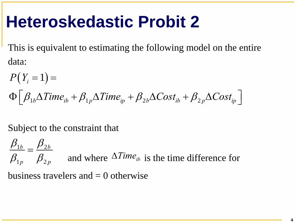
Heteroskedastic Probit 2This is equivalent to estimating the following model on the entire data:
( )
1 1 2 2
1i
b ib p ip b ib p ip
P Y
Time Time Cost Costβ β β β
= =
⎡ ⎤Φ Δ + Δ + Δ + Δ⎣ ⎦
Subject to the constraint that
1 2
1 2
b b
p p
β ββ β
= and where ibTimeΔ is the time difference for
business travelers and = 0 otherwise

5
Marginal Effects for Probit
In the linear model 0 1i i iY Xβ β υ= + + we can interpret 1β
as the marginal impact of X on ( )0 1( | ) ii i
i
XE Y X Xβ β∂ += ∂ which
doesn’t depend on X or 0β . But in the Probit model: ( ) ( )0 1
0 1 1( | ) ii i
ii i
XE Y X XX Xβ β φ β β β∂Φ +∂ = = +∂ ∂
Note that this depends on X and 0β and takes its maximum value where 0 1 0iXβ β+ = . Note that:
( )( ) ( )0 1 1 0 1 1( )i iE X E Xφ β β β φ β β β+ ≠ +

6
Marginal Effects for logitRecall that for the Logit Model the probability of Y=1:
F(β0 + β1X) = 0 1( )
11 Xe β β− ++
The marginal effect is given by:
( )( )
0 10 1
0 1
( )( )
12( )
0 1 0 1 1
1( | ) 1
1
( ) 1 ( )
XXi i
Xi i
eE Y X eX X e
F X F X
β ββ β
β ββ
β β β β β
− +− +
− +
⎛ ⎞∂ ⎜ ⎟∂ +⎝ ⎠= =∂ ∂ +
= + − +
Note that this also depends on X and 0β and takes its maximum value where 0 1 0iXβ β+ = .

7
Multinomial (or Conditional) Logit
Suppose that household i chooses one out of a set of vehicles j (j = 1, …,J):
( ) ( ), , Extreme Valueij ij ij ij ijU V x iidβ ε ε= + ∼ The probability that household i choose alternative j is
( ) 0for all ij ikP U U j k− ≥ ≠ If ij ijV xβ= then scale of parameters is not identified. iid assumption is strong and implies Independence from Irrelevant Alternatives.

8
Advantages of MNL1. Likelihood function is globally concave so maximum
likelihood is easy for even large models. 2. IIA property allows sampling of alternatives in
situations with very large number of discrete alternatives (for example, multi-car household vehicle choice).
3. Prediction and welfare calculations are straightforward and do not require “predicting” random utility components.
9
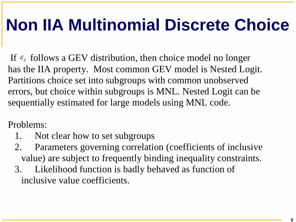
Non IIA Multinomial Discrete Choice
If ijε follows a GEV distribution, then choice model no longer has the IIA property. Most common GEV model is Nested Logit. Partitions choice set into subgroups with common unobserved errors, but choice within subgroups is MNL. Nested Logit can be sequentially estimated for large models using MNL code. Problems:
1. Not clear how to set subgroups 2. Parameters governing correlation (coefficients of inclusive
value) are subject to frequently binding inequality constraints.3. Likelihood function is badly behaved as function of
inclusive value coefficients.

10

11
Mixed logit: General distribution for η and extreme value for ε
Ui = β′xi + [ηi +εi]
U=β′X+[η+ε] where V(ε)=αI with known (i.e.,
normalized) α and V(η) is general
Density of η is f(η|Ω), where Ω are the fixed
parameters of the distribution.

12
Given η, the conditional choice probability is simply logit:
Li(η) = exp(β′xi + ηi) / ∑jexp(β′xj + ηj)
the unconditional choice probability is:
Pi=∫Li(η) f(η|Ω)dη
this is approximated by:
SPi = (1/R) ∑r=1,...,R Li(ηr)
Estimate by Max simulated log-likelihood function:∑nln(SPni)

13
•SPi is an unbiased estimate of Pi for any R
•Variance decreases as R increases
• It is strictly positive for any R, such that
ln(SPi) is always defined
• It is smooth (i.e., twice differentiable)
•The simulated probabilities sum to one over
alternatives, which is useful in forecasting.
•McFadden and Train have shown that any
random utility model can be approximated by
mixed logit

14
LM tests for Mixed Logit
( )2Cninin xxz −=
∑= j jnjnCn Pxx
Hypothesis of no random coefficients on attribute x is rejected if coefficient of z significantly different from zero

15
Mixed Logit Problems1. Mixed Logit likelihood can be very badly behaved so that
most applications use independent error components. 2. Estimates may be sensitive to simulation methods and
number of draws. 3. Identification can be very tricky (see M. Ben-Akiva and J.
Walker). 4. If the model is used for forecasting, there is the problem of
forecasting the random parameters for new observations and/or alternatives. Bottom line – use Mixed Logit LM tests as a specification test for MNL – try hard to find a good MNL specification!

16
Bayesian Discrete Choice
• Provide a principled approach for incorporating non-sample information
• Provide finite sample inference• Easy handling of model uncertainty• Parameters are random variables instead of fixed
constants

17
Prior distribution ( )θπ Likelihood function :
( )θ|xf Observe data and get posterior distribution:
( ) ( ) ( )( ) ( ) ( )∫
=θθπθ
θπθθdxf
xfxp|
||
In many cases the posterior mean is the optimal estimator. The key problem is computing high-dimensional integrals.

18
• Bayes confidence intervals• fixed regions containing θ with specified
coverage probability• conditions on observed data
• Classical confidence intervals• region with random endpoints containing true θ
over independent repeated replications of the data
• depends on distribution of unobserved realizations of the data

19
Bayesian Model UncertaintySuppose there are M competing models, and let
mπ Be the prior probability that model m is correct
( ) ( ) ( )∫= θθθ d| mmm pxfxf
( )( )∑
=
= M
jjj
mmm
xf
xf
1
π
ππ
Marginal density
Posterior probability that model m is correct

20
Unless there is a clear correct model, it is better to average over competing models :
( ) ( )∑=
=M
jjj xpxp
1
|| θπθ
The competing models do not need to be nested, and each model can be analyzed separately.
This only makes sense if you are averaging something with the same meaning (marginal effect or policy simulation!)

21
Bayesian computation:
Posterior distributions for discrete choice models (other than conditional logit) cannot be computed in closed form.
Use Markov Chain Monte Carlo methods to simulate draws from posterior distributions. The output files from these simulations can be saved and used to generate predictions. They can be reweighted to approximate the impact of changing prior distributions.

22
Bayesian Mixed Probit (Allenby and Rossi, 99)
( ) ( ) ( ) ( ) ( )βπθπθηπβηθβη |,||,, iii xfxp ∝
f is likelihood for multinomial probit, iη
is random effect for observation i. θ are the parameters of the distribution of the random effects over the sample. This Bayesian formulation permits inference for the individual effects (repeated SP experiments). Revelt and Train (1999) also give classical methods.
23
Poorly Identified Models:
Likelihood function will be almost flat, so classical
methods will have trouble converging to the optimum.
If proper prior distributions are used, Bayesian
methods will have no computational problems, but
posterior will look like prior for poorly identified
parameters. There are no problems for inference on
well-identified parameters.

24
Measurement Error:Discrete choice applications in transportation are
plagued by serious measurement errors. It is very
difficult to directly observe key variables for unchosen
alternatives, so it is common practice to impute travel
times and costs from network models. Unfortunately
this practice yields inconsistent parameter estimates
and overstates the precision of these estimates.

25
Multiple Imputations:General method for consistent inference using imputed values for missing or erroneous observations.
If the imputed values are somehow produced to match the first two moments of the correct unobserved values, then standard estimation methods that treat the imputed values as if they are correct will yield consistent parameter estimates. Unfortunately the standard errors produced by this approach will be inconsistent and downward biased because they ignore the errors introduced by the imputation process.

26
Rubin (1987) proposed solving this problem by
independently drawing multiple imputed values. The
component of variance due to the imputation error is then
estimated by the variability of the estimates across the
different imputed data sets.
If no data are missing, we use estimator:
θ~ and covariance estimator Ω~

27
Draw m independent imputations and compute corresponding parameter and covariance estimators:
j~θ j
~Ωand Final estimates are given by:
∑= m m1=j j
~ˆ θθ ( ) ,+1+ˆ -1 BmU=Σ
( )( ) ( )1ˆ~ˆ~j1=j j −
′−−= ∑ mB m θθθθ
.~1=j j∑ Ω=
m mU

28
These final estimates are consistent for any fixed number
of imputations, and they only require estimation of the
model where all data are observed without error.
Multiple imputations can be drawn once and stored so
they can be used for estimating different models.

29
Proper multiple imputations:
Draw from the Bayesian posterior predictive distribution of
the missing values under a specified model.
Any proper imputation procedure must condition on all
observed data, and different sets of imputed values must be
drawn independently so that they reflect all sources of
uncertainty in the response process.
30
Ex. San Diego Congestion Pricing ExperimentSolo drivers can pay to use an eight-mile stretch of reversible high occupancy vehicle (HOV) lanes along Interstate Route 15 north of San Diego, California.
Per-trip fee for solo drivers is posted on changeable message signs upstream from the entrance to the lanes, and may be adjusted every six minutes to maintain free-flowing traffic conditions in the HOT lanes.
Carpoolers use HOT lanes for no charge.
Model mode choice as a function of cost and time savings

31
HO
T L
an
e T
ime
Sa
vin
gs
0
5
10
15
20
25 Loop Detector Floating Car

32
Use 5 days with both loop detector and floating car data to estimate an imputation model to predict missing floating car data. Then use multiple imputations to account for errors in imputation when estimating value of time from a conditional logit mode choice model.
First transform time savings to bound between 0 and 35 minutes:
⎟⎠
⎞⎜⎝
⎛⎟⎠⎞
⎜⎝⎛ −⎟
⎠⎞
⎜⎝⎛
351
35log tt

33
Dependent Variable: Logit of Floating Car Time
Savings
R2 = 0.90
Root MSE = 0.36
Independent Variables: Coef. Std. Err. t-Stat.
Logit of Loop Detector Time Savings × Minutes
Past 5:00 A.M.
0.0029 0.00031 9.3
Minutes Past 5:00 A.M. 0.222 0.0149 14.8
(Minutes Past 5:00 A.M.)2 -0.00138 0.000121 -11.4
(Minutes Past 5:00 A.M.)3 2.73E-06 2.91E-07 9.38
Toll -0.229 0.188 -1.22
Toll × Minutes Past 5:00 A.M. 0.00222 0.00126 1.77
Constant -11.4 0.52 -22.1

34
Value of Time ($/hour) Corrected Loop Data95th Percentile 108.70 105.6090th Percentile 72.12 73.6375th Percentile 31.30 35.2750th Percentile 18.71 23.3725th Percentile 10.30 16.5510th Percentile -20.72 14.43
5th Percentile -83.02 14.08Mean 25.63 32.64
Implied value of time saved from mode choice model

The Impact of Residential Density The Impact of Residential Density on Vehicle Usage and Energy on Vehicle Usage and Energy
ConsumptionConsumptionDavid Brownstone and Tom Golob
University of California [email protected]
http://www.economics.uci.edu/~dbrownst/JUESprawlV3final.pdf
36
How does residential density affect travel? • How can we quantify the impacts of urban land use
density for assessing impacts of “urban sprawl” and for evaluating densification policies
• Conventional measures:• household car ownership
• and, for all household members:• trip generation (under-reporting of walk trips?)• trip distances• mode choices

37
Potentially more useful measures• 1. Total travel distance by all household vehicles
• captures: car ownership, trip generation, mode choices, and trip distances
• 2. Total fuel usage on all vehicles• captures vehicle type choice and implicit choice of fleet fuel
efficiency
38
Must control for selectivity biases
• Different types of households choose to live in neighborhoods of varying densities
• long list of potentially relevant demographic and socio-economic variables
• Persons choosing different lifestyles also choose to live in neighborhoods of varying densities
• may not be fully captured by demographic and socio-economic variables
• These household effects influence travel simultaneously with density

39
Previous Literature
• Newman and Kenworthy, 1999• Bento et al. (2005) • Boarnet and Sarmiento (1998) • Bhat and Guo (2007) • Ewing and Cervero, 2001, and Badoe and Miller,
2000, give literature reviews.
40
Our approach to the problem• Make choice of residential density endogenous
• Simultaneous equations with two sets of endogenous variables
• residential density• annual mileage and fuel consumption
• Both sets explained by demographic and socio-economic variables
• The residential density variable affects the two travel variables
• Estimate as a simultaneous system

41
Simultaneous system: 3 endogenous variables
Total annual fuel consumption
Land use density
Total annual mileage
Exogenous effects
income
household structure
ages
number of workers
number of drivers
race and ethnicity
etc.

42
2001 U.S. National Household Transportation Survey (NHTS)
• annual mileage for all household vehicles
• fuel usage for all household vehicles
• census data on land use density
• 24-hour travel diaries for all members
• 28-day record of long-distance travel (50 mi.+)
• demographics and socio-economics
• http://nhts.ornl.gov/2001/index.shtml
43
2001 NHTS data
• Annual mileage for all household vehicles• derived from two odometer readings or imputed
• fuel usage for all vehicles• according to vehicle make, model and vintage• see: Schipper and Pinckney (2003), Supplementing the 2001 NHTS with
Energy-related Data (online)
• Census data on land use density• housing units per sq. mi. (block and tract levels)• population per sq. mi. (block and tract)• jobs per sq. mi. (tract level)

44
2001 NHTS sample
• National sample• about 26,000 households• 82% have complete data on fuel usage
• California subsample• 2583 households• 2079 (80%) have complete data on fuel usage
• Plus 9 add-ons for other areas• about 44,000 additional households• generally, no data on mileage and fuel usage

45
Mileage, fuel usage by residential density
0
200
400
600
800
1,000
1,200
1,400
<50 50-250 250-1k 1-3k 3-5k >5k
housing units per square mile in census block group
gallo
ns p
er y
ear
0
5,000
10,000
15,000
20,000
25,000
30,000
35,000
mile
s pe
r yea
r
total annual fuelconsumption
total annual mileage
15% 23% 31% 8% 7%15%Percent of sample:
46
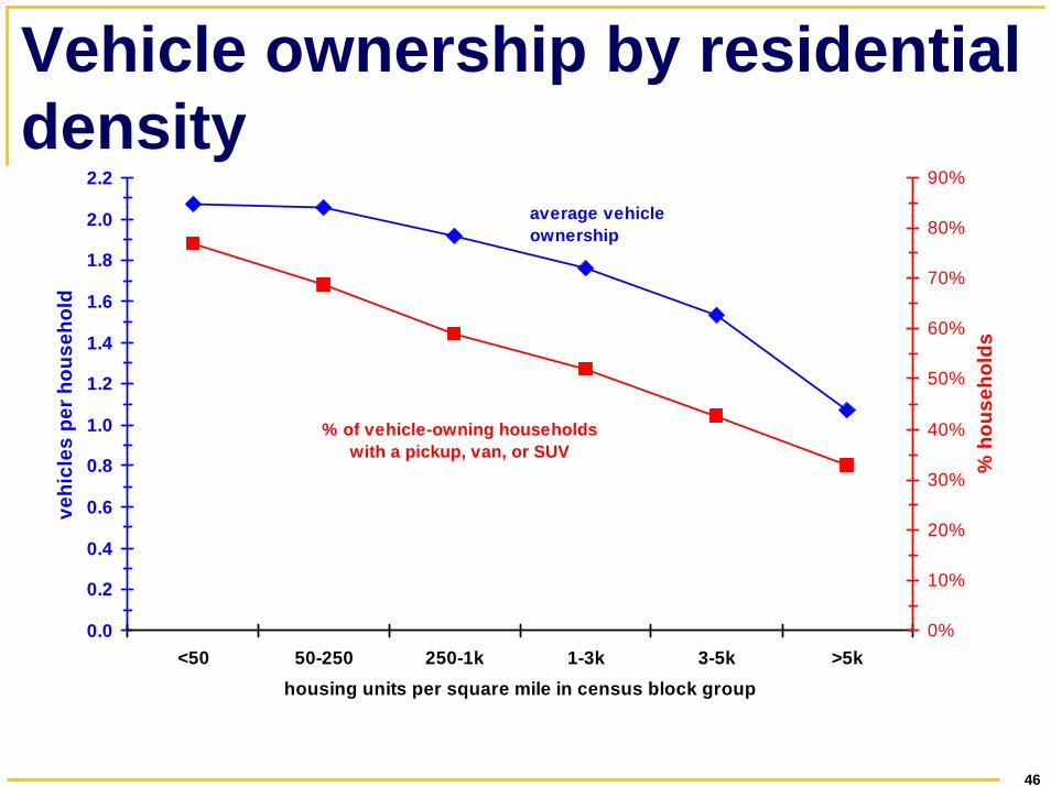
Vehicle ownership by residential density
0.0
0.2
0.4
0.6
0.8
1.0
1.2
1.4
1.6
1.8
2.0
2.2
<50 50-250 250-1k 1-3k 3-5k >5khousing units per square mile in census block group
vehi
cles
per
hou
seho
ld
0%
10%
20%
30%
40%
50%
60%
70%
80%
90%
% h
ouse
hold
s
average vehicleownership
% of vehicle-owning households with a pickup, van, or SUV

47
Demographics by residential density
0.0
0.5
1.0
1.5
2.0
2.5
3.0
<50 50-250 250-1k 1-3k 3-5k >5k
housing units per square mile in census block group
num
ber
0
10,000
20,000
30,000
40,000
50,000
60,000
70,000
$ U
Sdrivers per household
workers per household
household income

48
Mileage & fuel by vehicle type in single-vehicle households
0
100
200
300
400
500
600
700
800
900
1000
car van SUV pickup
type of vehicle in 1-vehicle h'holds (27% of unweighted U.S. sample)
gallo
ns p
er y
ear
0
2,000
4,000
6,000
8,000
10,000
12,000
14,000
mile
s pe
r yea
r
total annual fuelconsumption
total annual mileage
77% 8% 8%7%Percent of sample:

49
Mileage and fuel by vehicle type pairs in two-vehicle households
0
200
400
600
800
1,000
1,200
1,400
1,600
1,800
2 cars car & pickup car & van car & SUV 2 trucks
vehicle types in 2-vehicle h'holds (41% of U.S. sample)
gallo
ns p
er y
ear
0
5,000
10,000
15,000
20,000
25,000
30,000
mile
s pe
r yea
r
total annual fuel consumption
total annual mileage
30% 12% 15% 18%25%Percent of sample:

50
Important exogenous variables• Income• Number of drivers (continuous + dummy vars.)• Number of workers (continuous + dummy vars.)• Number of children (plus dummy for child > 15)• Education (2 dummy vars.)• Single-person household dummy• Retired household dummy• Race/ethnicity (4 dummy vars.)

51
Weighting to account for missing data
0
2,000
4,000
6,000
8,000
10,000
12,000
0 1 2 3 4 5 6+
vehicle ownership
Full energy data
Missing energy data

52
Biases due to missing data
• Missing data strongly related to number of vehicles, and this is closely related to endogenous mileage and fuel usage
• Sample selection problem• Structural approach (Heckman, 1979 Econometrica)
• Weighting (Manski and Lerman, 1977, Econometrica) – use WESMLE

53
Endogenous Missing Data
• Structural (Heckman) approach results are very sensitive to model specification.• But cannot reject hypothesis that missing data are
exogenous for preferred specification.• WESMLE is not efficient, but is less sensitive to
model specification. Also allows easy implementation of error heteroskedasticity.

54
WESMLE
• Model is
• WESMLE is
weight is inverse of probability of selection
( ) Ω=++=
i
iiii
CovBxAyy
εε
( )( ) ( )( )iiiii BxyAIBxyAIw −−Ω′
−− −∑ 1min

55
• WESMLE easy to compute, but variance=
⎟⎠⎞
⎜⎝⎛
⎟⎠⎞⎜
⎝⎛
′∂∂
⎟⎠⎞⎜
⎝⎛
∂∂=Λ
⎟⎠⎞
⎜⎝⎛
′∂∂∂−=Ψ
ΛΨΨ= −−
θθ
θθ
θθθ
)x,(L)x,(L
)x,( L
niiiii
iii2
11
ww
w
V
E
E
Alternative: Bootstrap – we used Wild Bootstrap to get covariance estimator that is consistent under arbitrary error heteroskedasticity

56
Wild Bootstrap
• Estimate model and get residuals, μi.• Multiply vector μi by a draw from
( ) ( ) ( )( ) ( ) ( )5251-1 PRwith251
5251 PRwith25-1
+=+
+=
Add resulting bootstrap residual to yi to get bootstrap samples

57
Specification testing• Reduced form:
• Structural restrictions:
iii Cxy μ+=
( )
( ) ( ) ( ) 11
1
−−
−
−Ω′
−=
−=
AIAICov
BAIC
iμ
Bootstrap variance of difference between restricted and unrestricted estimates of C

58
Is this algebra important?
• Wrong standard errors for WESMLE are between 10 –1000% downward biased.
• WESMLE estimates are statistically and operationally significantly different from unweighted estimates in many specifications.
• Standard overidentification tests reject many structural models that are accepted by bootstrap test – but bootstrap test does reject many specifications.
59
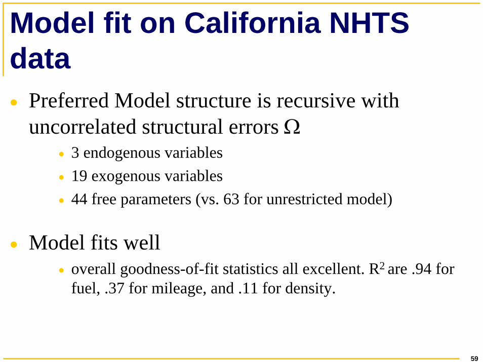
Model fit on California NHTS data• Preferred Model structure is recursive with
uncorrelated structural errors Ω• 3 endogenous variables• 19 exogenous variables• 44 free parameters (vs. 63 for unrestricted model)
• Model fits well• overall goodness-of-fit statistics all excellent. R2 are .94 for
fuel, .37 for mileage, and .11 for density.

60
Annual household fuel consumption in gallons 1173 1201
Total mileage per year for all household vehicles
25018 28486
Thousand dwelling units per sq. mile - Census block group
2.61 1.91
Annual household income in units of $10,000 7.08 5.66
Number of children in household 0.69 1.07
Number of workers in household 1.43 1.08
Number of drivers in household 1.86 1.03
Variable Mean Std. Dev.

61
Structural Parameter EstimatesCausal endogenous variable
Influenced endogenous variable Dwelling units per sq. mile in units of 1,000 –census block group
Total mileage per year on all household vehicles
Total mileage per year on all household vehicles
-1171(-4.97)
Household fuel usage per year in gallons
-20 (Total -65)(-5.12)
0.0382(17.3)

62
Restricted reduced form
Endogenous variable
Exogenous variable fuel usage mileage Density
Income in units of $10,000 24.2 276 -0.017
Number of children in household 55.0 271 -0.232
Number of workers in household -129 -211 0.180
1-worker household 422 8493
2-worker household 761 13316
3-or-more-worker household 1274 23327

63
Exogenous variable fuel usage mileage Density
Number of drivers in household 596 13815 -0.1391-driver household -128 -3716 -0.7012-driver household -315 -8792 -1.0133-or-more-driver household -265 -7515 -1.078
respondent has only college degree -45.9
respondent has postgraduate degree -74.9

64
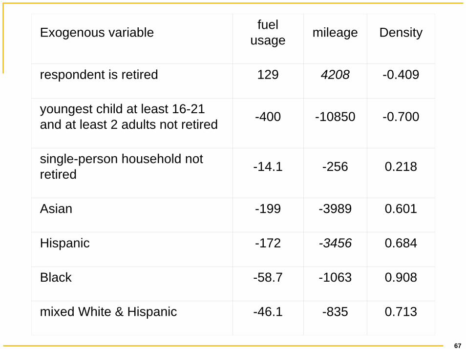
Exogenous variable fuel usage mileage Density
respondent is retired 129 4208 -0.409youngest child at least 16-21 and at least 2 adults not retired -400 -10850 -0.700
single-person household not retired -14.1 -256 0.218
Asian -199 -3989 0.601Hispanic -172 -3456 0.684Black -58.7 -1063 0.908mixed White & Hispanic -46.1 -835 0.713

65
Endogenous variable
Exogenous variable fuel usage mileage Density
Income in units of $10,000 24.2 276 -0.017
Number of children in household 55.0 271 -0.232
Number of workers in household -129 -211 0.180
1-worker household 422 8493
2-worker household 761 13316
3-or-more-worker household 1274 23327

66
Exogenous variable fuel usage mileage Density
Number of drivers in household 596 13815 -0.139
1-driver household -128 -3716 -0.701
2-driver household -315 -8792 -1.013
3-or-more-driver household -265 -7515 -1.078
respondent has only college degree -45.9
respondent has postgraduate degree -74.9
67
Exogenous variable fuel usage mileage Density
respondent is retired 129 4208 -0.409
youngest child at least 16-21 and at least 2 adults not retired -400 -10850 -0.700
single-person household not retired -14.1 -256 0.218
Asian -199 -3989 0.601
Hispanic -172 -3456 0.684
Black -58.7 -1063 0.908
mixed White & Hispanic -46.1 -835 0.713

68
Contrasting results for 3 NHTS samples• National
• N = 21,347
• Portland Metro Area and rest of Oregon• (includes 2 counties in WA)• N = 325
• California• N = 2,079

69
0%
5%
10%
15%
20%
25%
30%
35%
40%
45%
0-50 50-250 250-1k 1-3k 3-5k 5k+Housing units per square mile
USACAOR
Residential densities for 3 NHTS samples

70
Results by areaIncrease in density of 1,000 households / sq. mi. (40%)
Change in annual fuel consumption due to:Change in annual
total mileage on all household
vehicles mileage fuel economy Total
U.S. - 1,630 - 74 - 16 - 90OR - 1,340 - 57 - 20 - 77
CA - 1,200(4.8%) - 45 - 20 - 65
(5.5%)
71
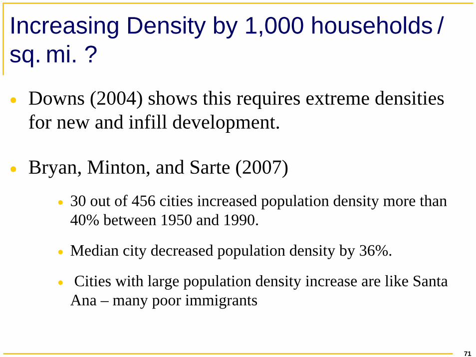
Increasing Density by 1,000 households /sq. mi. ?
• Downs (2004) shows this requires extreme densities for new and infill development.
• Bryan, Minton, and Sarte (2007)• 30 out of 456 cities increased population density more than
40% between 1950 and 1990.
• Median city decreased population density by 36%.
• Cities with large population density increase are like Santa Ana – many poor immigrants

72
Conclusions
• We can measure the effects of residential density controlling for residential choice (self-selection)
• Self-selection effects are fully captured by rich demographics
• Impact of increased density statistically significant but too small for useful policy.

73
Vehicle Type Choice
• Previous results suggest that density may be related to the choice of vehicle fuel efficiency.
• Except for Bhat and Guo (2007) previous literature has treated density as exogenous
• Standard discrete choice has curse of dimensionality in number of vehicles.

74
BMOPT model with endogenous density• Extends Fang’s (2008) Bayesian Multivariate
Ordered Probit and Tobit model to include an equation for density. Can be easily estimated with standard MCMC methods.
• Reduced form alternative to Bhat (2005) MCDEV model. This requires that the total household miles driven is fixed.

75
BMOPT Model
ii ii Dy xα β ε∗ = + + (1)
ii iD zγ η= + (2)
where iy∗ is a 4 by 1 vector of latent dependent variables for number of cars,
number of trucks, mileage on cars, and mileage on trucks; iD is a measure of density for households i at the census tract level, and is endogenous. Therelation between the latent dependent variables and their observed values are:
0
0 1
0 if 1 2
1 if 1 2
2 otherwise 1 2
if 0 3 4
0 otherwise 3 4
j j
j j
j
j j j
j
y y j
y y j
y j
y y y j
y j
α
α α
∗
∗
∗ ∗
= , ≤ , = ,
= , < ≤ , = ,
≥ , , = ,
= , > , = ,
= , , = ,

76
Data and Estimation
• Use a random subsample of 5863 observations from 2001 NHTS (25,027 total observations).
• Use MSA density as instrument for census block level density (appears strong 1st stage F-statistic about 400).
• Do out of sample forecasting tests from subsample to the remainder of the NHTS data.

77
Change in Vehicle Ownership for 50% increase in density
Probability changes for truck choice Δ P(tnum=0) Δ P(tnum=1) Δ P(tnum≥2)
.0267 -.0107 -.0159 (.0058) (.0023) (.0035)
Probability changes for car choice
Δ P(cnum=0) Δ P(cnum=1) Δ P(cnum≥2) -.0047 .0005 .0042 (.0054) (.0007) (.0048)

78
Change in Vehicle miles for 50% increase in density
Δ car miles %Δ car miles Δ truck miles %Δ truck miles
14.02 .16 -610.5 -8.27 (196.79) (2.23) (117.66) (1.59)

79
Out of Sample Predictions
c=0 c=1 c ≥ 2 t=0 t=1 t ≥ 2 Predicted number
of households 1301 2677 1013 2413 1774.6 804
(standard deviation)
(28.8) (33.8) (25.5) (29.7) (34.9) (25.9)
True number of households
1060 2601 1330 2165 1884 942
average miles by cars
average miles by trucks
Forecast 9113.6 7649.3 (standard deviation) (178.9) (210.6)
True 9135 7204.4

80
Conclusions
• No evidence for self-selection bias after controlling for rich sociodemographics
• BMOPT model works well and does tolerably well in out of sample forecasting
• Impact of increased density statistically significant but too small for useful policy.