a comprehensive study and mechanism investigation …
TRANSCRIPT

A COMPREHENSIVE STUDY AND MECHANISM INVESTIGATION FOR
ALKALINE-HEAVY OIL RECOVERY PROCESS
A Thesis
Submitted to the Faculty of Graduate Studies and Research
In Partial Fulfillment of the Requirements
For the Degree of
Master of Applied Science
in
Petroleum Systems Engineering
University of Regina
By
Zhiyu Xi
Regina, Saskatchewan
December, 2019
©copyright 2019-Zhiyu Xi
UNIVERSITY OF REGINA
FACULTY OF GRADUATE STUDIES AND RESEARCH
SUPERVISORY AND EXAMINING COMMITTEE
Zhiyu Xi, candidate for the degree of Master of Applied Science in Petroleum Systems Engineering, has presented a thesis titled, A Comprehensive Study and Mechanism Investigation for Alkaline-Heavy Oil Recovery Process, in an oral examination held on December 3, 2019. The following committee members have found the thesis acceptable in form and content, and that the candidate demonstrated satisfactory knowledge of the subject material. External Examiner: Dr. Amr Henni, Industrial Systems Engineering
Supervisor: Dr. Na Jia, Petroleum Systems Engineering
Committee Member: Dr. Farshid Torabi, Petroleum Systems Engineering
Chair of Defense: Dr. Yiyu Yao, Department of Computer Science

i
ABSTRACT
Alkaline flooding is an important branch of chemical enhanced oil recovery (EOR).
The complexity of alkaline flooding study is mainly embodied by its chemical reaction
required by alkalis to react with oil acids. Consequently, in-situ surfactants are
generated for various emulsification phenomenon. It is known that alkaline flooding
performance in oil recovery is subjected to the emulsion type generation, thus, of great
importance to alkaline flooding study is its mechanism investigation and saponification
rate examination.
In this study, a modified bottle test method that assesses major emulsion type formation
for preliminary prediction of alkaline flooding performance in oil recovery is
introduced. Homogenization and Karl-Fischer water content titration techniques were
applied in the modified bottle test to overcome the emulsion preparation and analysis
difficulties. In addition, sandpack alkaline flooding tests were conducted to prove the
prediction reliability of the modified bottle test through identifying effluent emulsions.
It is found either water in oil emulsion or oil in water emulsion could be
representatively prepared in bottle test based on reaction environments identical to
flooding tests’ conditions. Taking advantages of bottle test’s superior efficiency in
simultaneous multi-case study, alkaline flooding screening test can be easily conducted
applying statistical techniques to provide prior visions regarding dominating driving
mechanism of oil recovery. This research verified a practical solution to representative
emulsion preparation and phase volume quantification in the bottle test especially when
it comes to high viscous heavy oil; therefore, mechanism investigation regarding
alkaline flooding could be easily conducted.
Besides, the CMGTM alkaline flooding simulation model was built considering the
saponification reaction rate of immiscible fluids. A novel experiment design of alkali-

ii
heavy oil reaction system was proposed and implemented to measure reagents’ reaction
rate at various temperatures through monitoring pH change by electrode. Through
which the Arrhenius constant and activation energy were calculated. In addition, the
stoichiometry for emulsification reaction was proposed according to bottle test results.
The simulation model was history matched founded on reaction data thus model
uncertainty was mitigated by reducing number of unconstrained parameters. Oil
recovery predictions have been conducted using the history matched model and the
optimized injection strategies were addressed.

iii
ACKNOWLEDGEMENTS
I would like to express my great gratitude to my supervisor, Dr. Na (Jenna) Jia, for her
full support on my research work without any reservation. Her passionate attitude and
perseverance in discovering scientific findings and solving engineering problems
always encourage me to learn more and work harder. She never stopped igniting the
sparkle of thoughts when I reached the dead end of the research and guiding me back
to the right track with wise advices.
I would also like to express my appreciation to all the committee members, Dr. Amr
Henni, Dr. Farshid Torabi who have spent their precious time to review my thesis and
providing constructive suggestions.
Finally, I would like to acknowledge PTRC and Mitacs Accelerate programs for their
financial support to support my research works and provide me the precious internship
opportunities to cultivate my professional working attitude and research skills.

iv
DEDICATION
For my parents Mr. Hao Xi and Mrs. NingRong Li, and my wife Yalu. In memory of
my grandpa, who was my life mentor from an early age.

v
Table of Contents
ABSTRACT .................................................................................................................. i
ACKNOWLEDGEMENTS ...................................................................................... iii
DEDICATION ............................................................................................................ iv
List of Tables ..............................................................................................................vii
List of Figures .......................................................................................................... viii
Nomenclatures ............................................................................................................ xi
CHAPTER 1: Introduction and Literature review .................................................. 1
1.1 Heavy oil recovery in Canada ............................................................................................1
1.1.1 Heavy oil recovery challenges.................................................................................1
1.1.2 Heavy oil recovery methodology ............................................................................5
1.2 Alkaline flooding in Canada ...............................................................................................6
1.2.1 Driving mechanisms ................................................................................................6
1.2.2 Synergy of alkaline flooding with other EOR methods ...........................................9
1.3 Research Objectives .........................................................................................................10
1.3.1 Improvement of alkaline flooding driving mechanism prediction ........................10
1.3.2 Introduction to enhanced alkaline flooding simulation .........................................13
CHAPTER 2: Experiment design, workflow and fundamental theories ............. 16
2.1 Modified screening bottle test ..........................................................................................16
2.2 Sand pack flooding test ....................................................................................................25
2.3 Chemical reaction rate test ...............................................................................................27
2.3.1 Chemical reaction frequency factor theory ...........................................................27
2.3.2 Experiment design of reaction rate test .................................................................30
CHAPTER 3: Experiment works and results ........................................................ 33
3.1 Gas chromatography (GC) ...............................................................................................33
3.2 Fourier-transform infrared spectroscopy (FTIR) ..............................................................42
3.3 Karl Fischer volumetric water content titrator .................................................................46

vi
3.4 pH/ion meter neutralization reaction rate test ..................................................................48
3.5 Cone and plate viscometer and capillary method .............................................................58
3.6 Spinning drop tensiometer................................................................................................61
CHAPTER 4: Alkaline flooding driving mechanism investigation ...................... 67
4.1 Modified screening bottle test ..........................................................................................67
4.2 Sand pack flooding test ....................................................................................................88
CHAPTER 5: Enhanced Numerical Simulation of Alkaline Flooding .............. 105
5.1 Preliminary alkaline flooding model .............................................................................. 108
5.1.1 Basic settings of preliminary alkaline flooding model ........................................ 108
5.1.2 Sensitivity analysis of alkaline flooding model ................................................... 112
5.2 History matched alkaline flooding simulation ............................................................... 122
5.2.1 Alkaline flooding prediction and optimization .................................................... 122
5.2.2 Alkaline flooding model considering multivalent cation effects ......................... 128
5.2.3 Limit of current alkaline flooding model ............................................................ 140
REFERENCES ........................................................................................................ 146
APPENDICES ......................................................................................................... 151

vii
List of Tables
Table 1. Heavy oil compositional analysis results up to C90+ .............................. 41
Table 2. Neutralization reaction rate measured at 6 temperatures ....................... 52
Table 3. Viscosity measured by cone and plate viscometer ................................ 60
Table 4. Modified bottle test orthogonal experiment designs of two alkalis ....... 69
Table 5. NaOH orthogonal bottle test material balance calculation .................... 71
Table 6. Na2CO3 orthogonal bottle test material balance calculation ................. 71
Table 7. Orthogonal experiment data processing for 2 alkalis ............................ 72
Table 8. NaOH bottle test trend study design ...................................................... 75
Table 9. Volume corrected NaOH trend study results ......................................... 77
Table 10. Na2CO3 bottle test trend study design ................................................. 78
Table 11.Volume corrected Na2CO3 trend study results ...................................... 78
Table 12. Sandpack alkaline flooding test strategies ........................................... 88
Table 13. Marginal cost per PV alkaline injection ............................................ 127
Table 14. Two NaOH flooding sandpack properties comparison ..................... 129
Table 15. EXP6 effluent Ca2+ concentration change with time ......................... 134

viii
List of Figures
Figure 1. Oil trapping model (a) Jamin effect and (b) Pore-doublet model (Green
& Willhite, 2008) ........................................................................................... 3
Figure 2. Bottle test instruments: (a) High-shear homogenizer (b) KF auto titrator
...................................................................................................................... 18
Figure 3. Glass bottle used in bottle test, (a) Unmeasurable top and middle phase
volume and (b) Glass bottle with open-top lid and rubber septa ................. 21
Figure 4. Work flow of modified bottle test ........................................................ 24
Figure 5. Schematic diagram of sandpack alkaline flooding test ........................ 26
Figure 6. Reaction rate test setup ........................................................................ 32
Figure 7. Schematic diagram of Agilent 6890N GC ........................................... 34
Figure 8. Standard mix chromatographs (a) 6890N GC measured and (b)
reference chromatograph provided by Agilent ............................................. 37
Figure 9. Heavy oil sample chromatograph edited by Agilent ChemStation ...... 38
Figure 10. Simulated distillation result with boiling point distribution .............. 40
Figure 11. FTIR spectrum of pentane extracted asphaltenes from crude oil and oil
after neutralization reaction ......................................................................... 44
Figure 12. Schematic diagram of Karl Fischer titration system .......................... 47
Figure 13. Neutralization reaction tests at 27, 35 and 39.5 ℃ ............................ 50
Figure 14. Neutralization reaction tests at 42.5, 47 and 51 ℃ with 35 ℃
repeatability test ........................................................................................... 51
Figure 15. Arrhenius equation plot ..................................................................... 53
Figure 16. Precipitation reaction rate test at (a) 20 and (b) 40 ℃ ...................... 57
Figure 17. Droplet shape observation of (a) NaOH concentration and (b) salinity
effect tests..................................................................................................... 62

ix
Figure 18. IFT change with (a) NaOH concentration change and (b) salinity
change .......................................................................................................... 63
Figure 19. Droplet shape observation of (a) Na2CO3 concentration and (b) salinity
effect tests..................................................................................................... 64
Figure 20. IFT change with (a) Na2CO3 concentration change and (b) salinity
change .......................................................................................................... 65
Figure 21. Bottle test trend study phases at equilibrium after 24 hours .............. 75
Figure 22.Three emulsion phases distribution of bottle test trend study after
calibration starting from: (a) NaOH concentration trend study; (b) NaOH
salinity trend study; (c) Na2CO3 concentration trend study; (d) Na2CO3
concentration trend study ............................................................................. 80
Figure 23. Bottle test trend study oil volume expansion ratio starting from: (a)
NaOH concentration trend study; (b) NaOH salinity trend study; (c) Na2CO3
concentration trend study; (d) Na2CO3 concentration trend study............... 82
Figure 24. Optimum alkali concentrations measured by modified bottle test and
IFT ................................................................................................................ 85
Figure 25. Sandpack flooding test data starting from: (a) NaOH flooding oil
recovery factor; (b) Na2CO3 flooding oil recovery factor; (c) NaOH flooding
pressure drop; (d) Na2CO3 flooding pressure drop ...................................... 89
Figure 26. Emulsion type of effluent from sandpack .......................................... 92
Figure 27. Dimensionless shear rate and corresponding oil recovery every 10 min
during alkaline injection.. ............................................................................. 97
Figure 28. Sandpack flooding test effluents of (a) NaOH introduced W/O
emulsion and (b) Na2CO3 introduced O/W emulsion under microscopic view
...................................................................................................................... 99

x
Figure 29. Emulsion particle size distribution analysis..................................... 100
Figure 30. Water cut data of (a) NaOH flooding and (b) Na2CO3 flooding ...... 102
Figure 31. Reaction 1 enthalpy, Reaction 2 rate frequency and logarithm capillary
number sensitivity tests .............................................................................. 113
Figure 32. History matched relative permeability curves in (a) interpolation set 1
and (b) interpolation set 2 .......................................................................... 117
Figure 33. History match process in sequence of relative permeability, reaction 2
rate frequency and reaction 1 enthalpy ...................................................... 118
Figure 34. Comparison of simulation results and experiment data ................... 119
Figure 35. Oil bank formation and Sor reduction during alkaline flooding ....... 121
Figure 36. Simulation results by escalating concentration NaOH flooding ...... 123
Figure 37.Simulation results by different PV of NaOH injection ..................... 126
Figure 38. Comparison of NaOH flooding results of EXP3 and EXP5 ............ 130
Figure 39. Comparison of NaOH flooding results of EXP5 and EXP6 ............ 132
Figure 40. (a) Ion concentration experiment setup and (b) history match results
.................................................................................................................... 135
Figure 41. CaCl2 effects on oil recovery by NaOH flooding ............................ 137
Figure 42. CaCl2 mole fraction in produced water of different preflush cases . 139
Figure 43. (a) Limit of NaOH flooding model and (b) Optimum prediction range
of PV NaOH injection by current simulation model .................................. 141

xi
Nomenclatures
Modified bottle test material balance:
Voi: initial oil volume, mL
Vwi: initial water volume, mL
Vo: measured oil-external emulsion volume, mL
Vw: measured water-external emulsion volume, mL
msao: bottle weight with oil and solution, g
msa: bottle weight with solution, g
ρoT: oil density at certain temperature, g/mL
ρw: water density, default, g/ mL
ρavg: overall density of a bulk phase after neutralization reaction, g/ mL
Vmcalc1: calculated emulsion phase volume by volume balance, mL
Vmcalc2: calculated emulsion phase volume by mass balance, mL
W%: water content in each bulk phase
Oil external emulsion water content calibration:
W%true: actual water content of oil-external emulsion
mb: mass of bottle
mbo: mass of bottle and oil sample
mboc: mass of bottle, oil sample and solvent
Dimensionless shear rate:
μ: Viscosity, cp
ΔP: Pressure drop, Mpa
Deff: Effective diameter of capillary, m
Q: Volumetric flow rate, m3/s
L: capillary length, m
xii
γactual: actual shear rate, s-1
γapparent: apparent shear rate, s-1
γdim: dimensionless shear rate
Hagen-Poiseuille’s equation:
v: sandpack fluid velocity, m/s
k: sandpack permeability, m2
φ: sandpack porosity
L: sandpack length, m
ΔP: pressure drop, mPa
μo: oil viscosity, mPa·s
Miscellaneous:
Aconc.: alkaline concentration, mol/L
Temp.: Temperature, ℃
Vo+m%: Middle water and top oil external emulsions volume fraction
PcL : left-hand capillary pressure
PcR : right-hand capillary pressure
PA : pressure at A end of capillary
PB : pressure at B end of capillary
σow : oil/water interfacial tension
θ : contact angle
r : capillary radius
Vmcalc1: middle emulsion volume calculated by volume balance, mL
Vmcalc2: middle emulsion volume calculated by mass balance, mL
1
CHAPTER 1: Introduction and Literature review
1.1 Heavy oil recovery in Canada
Canada is well rich in hydrocarbon resources. It has the world’s third largest proven
oil reserves, and it is also one of the world’s largest countries of oil exporter ("Oil
Resources" 2017). The oil recovery and refinery is an important pillar of Canadian
economy development. According to Natural Resources Canada annual energy report
in 2014, oil and gas market has occupied 7.5 % of total Canadian GDP and this value
is still increasing in recent years. The appropriate exploration, development and
distribution of hydrocarbon resources significantly impact the country prosperity.
Heavy oil, which is usually in form of bitumen or tar sands with high viscosity, takes
a considerable part (approximately 95%) among the oil reserves in Canada. Over 90%
of heavy oil reserves were found and developed in Alberta and Saskatchewan ("Oil
Resources" 2017). Unlike conventional oil, more efforts and new technologies are
required for enhancing the recovery of such unconventional resource. Due to the
technology limitation, there are still more than 60% of heavy oil untapped in the
formation waiting to be recovered. Therefore, the research of heavy oil recovery has
never been more popular than nowadays trying to exploit all necessary means to extract
the additional oil out of the formation.
1.1.1 Heavy oil recovery challenges
Heavy oil is named according to its natural fluid properties. Because heavy oil is
usually formed in shallow stratum 500 meters below the sea level at relatively low
pressure and temperature condition, its density is higher than conventional oil so be its
viscosity. Thus, it results in low solution gas storage and the unconsolidated sand
formation is not able to provide sufficient spontaneous rock expansion. The oil flow in
porous media is inferior to gas and brine which flow at higher mobility. This

2
contributes to the continuously declining oil recovery due to the dropping oil saturation
and trapped oil in the long run.
The oil phase trapping in the porous media is mainly due to three reasons which are
the pore structure of porous media, rock fluid wettability and IFT. Description of the
oil trapping considering fluid channel tortuosity will be quite tedious because of the
reservoir heterogeneity. Therefore, these three factors are combined into Jamin Effect
model that portrays how an oil phase is trapped inside the capillary media. Even though
Jamin Effect model is simplified, it still can explain the trapping mechanisms
essentially. As previously stated, the wetting phase will be trapped between solid
surface by interconnected fluid layers over a very long distance, while the non-wetting
phase trapping is usually in the form of isolated drops contributed by snap-off (Blunt,
2017) thus loses its driving motivation. Therefore, it is extremely inefficient to use a
non-wetting phase to displace a wetting phase. The following cases assume the
reservoir rock is water wet while the displaced oil phase is non-wetting phase.
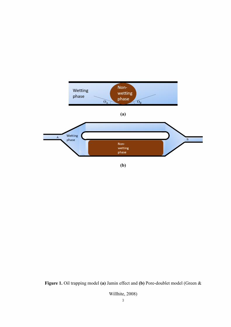
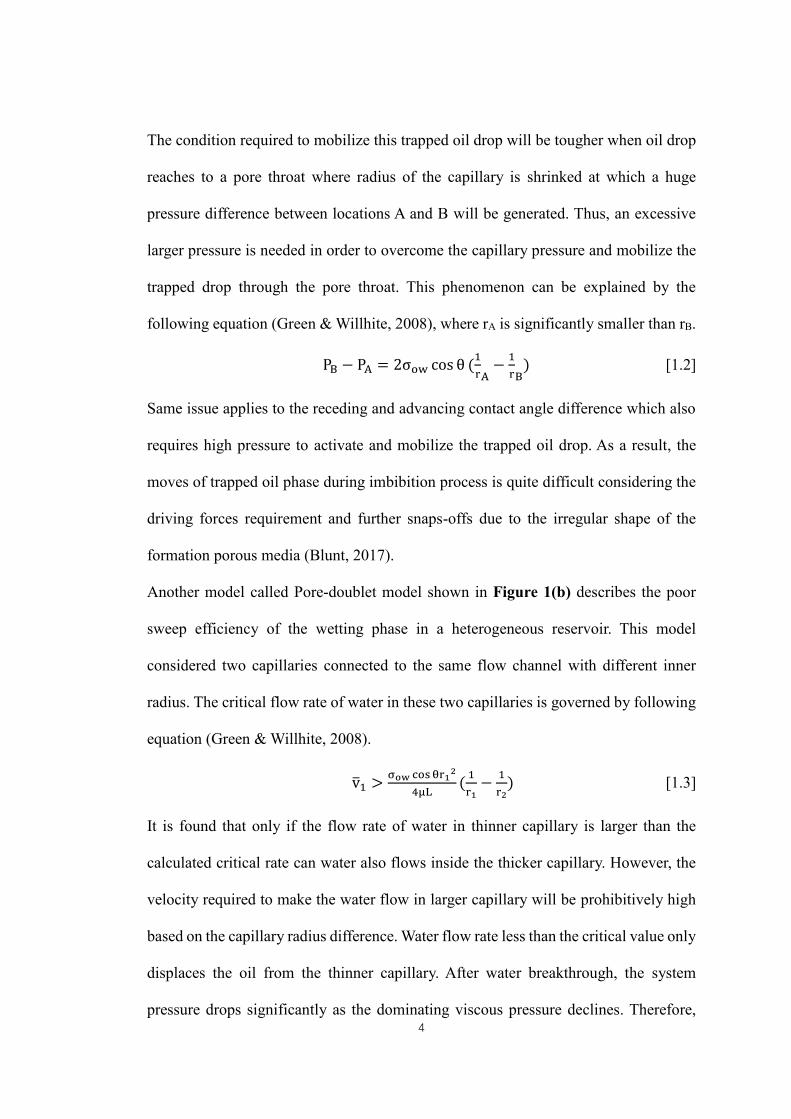
The first model illustrated in Figure 1(a) describes an oil drop trapped in the single
capillary with force balance which is represented by PA + PcL = PB +PcR, where the
viscous force and capillary force on both capillary ends are equal. Rearrange this
equation and the following equation can be derived (Green & Willhite, 2008):
PB − PA = (2σow cosθ
r)A − (
2σow cosθ
r)B [1.1]
For identical wettability and capillary in a homogeneous reservoir, there is no pressure
difference between the two sides of the trapped drop. Consequently, the drop will not
be mobilized until the application of other external forces.
3
(a)
(b)
Figure 1. Oil trapping model (a) Jamin effect and (b) Pore-doublet model (Green &
Willhite, 2008)
4
The condition required to mobilize this trapped oil drop will be tougher when oil drop
reaches to a pore throat where radius of the capillary is shrinked at which a huge
pressure difference between locations A and B will be generated. Thus, an excessive
larger pressure is needed in order to overcome the capillary pressure and mobilize the
trapped drop through the pore throat. This phenomenon can be explained by the
following equation (Green & Willhite, 2008), where rA is significantly smaller than rB.
PB − PA = 2σow cos θ (1
rA−1
rB) [1.2]
Same issue applies to the receding and advancing contact angle difference which also
requires high pressure to activate and mobilize the trapped oil drop. As a result, the
moves of trapped oil phase during imbibition process is quite difficult considering the
driving forces requirement and further snaps-offs due to the irregular shape of the
formation porous media (Blunt, 2017).
Another model called Pore-doublet model shown in Figure 1(b) describes the poor
sweep efficiency of the wetting phase in a heterogeneous reservoir. This model
considered two capillaries connected to the same flow channel with different inner
radius. The critical flow rate of water in these two capillaries is governed by following
equation (Green & Willhite, 2008).
v̅1 >σow cosθr1
2
4μL(1
r1−
1
r2) [1.3]
It is found that only if the flow rate of water in thinner capillary is larger than the
calculated critical rate can water also flows inside the thicker capillary. However, the
velocity required to make the water flow in larger capillary will be prohibitively high
based on the capillary radius difference. Water flow rate less than the critical value only
displaces the oil from the thinner capillary. After water breakthrough, the system
pressure drops significantly as the dominating viscous pressure declines. Therefore,

5
large amount of oil is bypassed inside the thick capillary. Generally, the oil production
at primary and secondary recovery stage is extremely limited and therein only 10 % to
20 % of original oil in place (OOIP) can be recovered.
1.1.2 Heavy oil recovery methodology
The heavy oil recovery process is mainly undergoing three stages. Initially, the primary
production automatically produces oil out of the reservoir by pressure depletion and
formation rock and reservoir fluids expansion (Kokal & Abdulaziz, 2010). However,
the primary recovery will not be long-lasting due to the reservoir pressure depletion
that fails to provide sufficient energy to overcome the viscous force generated by high
viscous nature of heavy oil and Jamin Effect. Water flooding as a secondary recovery
method is conducted afterwards to maintain reservoir pressure and mobilize the
residual oil. Nonetheless, the water with low viscosity as displacing fluid results in
unfavorably large mobility ratio. Severe viscous fingering usually occurs which
contributes to early water breakthrough and high residual oil saturation (Sor) in porous
media (Homsy, 1987; Bryan & Kantzas, 2007). Where Sor indicates the maximum oil
can be recovered. The difficulties of primary and secondary oil recovery have been
explained theoretically in previous Chapter 1.1.1. In order to recover more oil, in other
words, reduce Sor, various enhanced oil recovery (EOR) approaches can be
implemented following water flooding. Most of the EOR processes focus on scaling
down the mobility ratio or reducing IFT thus further diminish the Sor. These goals can
be achieved by incorporating solvent injection, thermal treatment as well as chemical
treatment to purposely recover additional 10% original oil in place (OOIP) or higher
from the reservoir (Kokal & Abdulaziz, 2010).

6
1.2 Alkaline flooding in Canada
As one of the chemical EOR processes, alkaline flooding has numerous merits in oil
recovery which is mainly represented by its low cost (Ding, Zhang, Ge & Liu, 2010)
and high versatility to post water treated oil reservoir. Different from the conventional
surfactant flooding that directly introduces artificial surfactants into the reservoir,
alkalis like sodium hydroxide and sodium carbonate react with the acidic components
of the residual oil and spontaneously generate surfactants in-situ (Ashrafizadeh,
Motaee & Hoshyargar, 2012; Rivas, Gutierrez, Zirrit, Anto’n & Salager, 1997). This
phenomenon majorly relies on the neutralization reaction between the alkalis and fatty
acids of oil. Thus, the total acid number (TAN) of oil becomes an important index that
implies the alkaline flooding feasibility in a certain reservoir. Acevedo, Escobar,
Gutiérrez and Rivas (1992) have concluded that majority of carboxylic acid groups in
oil is contributed from asphaltenes contents, phenols or resins of oil which are known
to be rich in heavy oil. The average asphaltenes contents of Alberta heavy oil is usually
15 wt% according to several heavy oil SARA test reports from commercial labs.
Moreover, the strong natural polarity of asphaltenes is capable of fortifying the
emulsion stability (Dehghan, Masihi & Ayatollahi, 2013). These advantages enable
alkaline flooding to be a good candidate for unconventional heavy oil recovery in
Canada (Bryan & Kantzas, 2007; Ashrafizadeh et al., 2012; Acevedo, Gutierrez &
Rivas, 2001).
1.2.1 Driving mechanisms
There are four major driving mechanisms working collaboratively to facilitate the oil
recovery, which are subjected to the varying emulsion types in alkaline flooding
(Johnson, 1976). The emulsification process is necessary to be thoroughly explained

7
before the discussion of alkaline flooding driving mechanisms. As mentioned
previously, the alkalis react with heavy oil components to generate surfactants in-situ.
Those formed surfactant molecules disperse into the solvent as monomers and also
occupy the interface of the immiscible fluids initially. Then, the molecules gradually
aggregate with increasing surfactant concentration. As the concentration of surfactant
reaches the critical micelle concentration (CMC), micelle is formed in spherical shape
with their hydrophilic ends facing outward if the solvent is water. For organic solvent,
vice versa. Surfactant concentration exceeds CMC leads to further micelle aggregation
but has little influence to initially dispersed monomers on the interface. These micelles
have good solubility within the oil or water phase depend on their types. Thus, even
though water and oil are immiscible phases, they can still be mutually dissolved with
each other and the dispersed phase will be stabilized by electrical repulsion contributed
by the surfactants (Green & Willhite, 2008). This process is so called emulsification.
Remind that interfacial tension is the force per unit length which is required to create
additional surface area. When two immiscible fluids become dispersible, the IFT
between those two fluids drops significantly which is indicated by the increase of
water/oil interfacial area.
Water/oil IFT is determined by surfactant concentration and the IFT has to be low
enough in order to acquire a stable emulsion. Taber number is the index used to
quantify the maximum IFT threshold required to form a stable emulsion thus a
reasonable oil production could be achieved. This number is in the order of 6 (Pitts, et
al., 2004). It has to be at least 30 for alkaline flooding or other IFT reduction targeted
EOR methods for purpose of reducing residual oil saturation significantly, in other
words, generating more stable emulsion. If a typical reservoir has maximum pressure
gradient of 0.5 psi/ft, then, the IFT needs to be dropped to 10-2 dyne/cm in order to

8
achieve a proper oil recovery.
ΔP
Lσ= 30(
psi
ft)/(
dynes
cm) [1.4]
The IFT falls in the range from 10-2 dyne/cm to 10-5 dyne/cm is also called ultralow
interfacial tension.
The emulsions formed in the formation normally have 2 major types, water in oil
emulsion (W/O) and oil in water emulsion (O/W) respectively, which contribute to the
first two driving mechanisms of alkaline flooding. The first driving mechanism is
emulsification and entrainment, for the scenario of fine oil droplets are dispersed in the
water phase and flow with water as one pseudo-phase flow. In this case, previously
unmovable oil bulks are gradually grinded into small particles and flow with water.
This type of emulsion has close viscosity to water which makes it ease at flow. The
second mechanism is called emulsification and entrapment, which illustrates that large
dispersed phase particles in the emulsion block the pore throat of the dominating flow
channel when the emulsion passes through. It usually occurs in the scenario of forming
water in oil emulsion since the average size of the dispersed water droplets is larger
than that of the oil droplets in the water external emulsion. Some researchers also
reported that minor oil droplets in the water external emulsion may block the pore
throat and results in improvement of the areal sweep efficiency. The rest two
mechanisms are related to wettability alteration including water-wetting to oil-wetting
or oil-wetting to water-wetting, which is case specific according to original formation
wettability condition. The oil retention on the oil-wetting rock surface and continuous
water film along porous channel in water-wetting formation are key facts that restrain
the oil production. Altering the rock wettability mitigates the preferential flow channel
effect (continuous water phase) in the flow system therefore facilitates the areal sweep
efficiency and contributes to additional oil recovery. As is mentioned in last section,
9
the trapped oil forms unmovable portion in a water-wetting rock due to the formation
of water preferential channel. Nonetheless, if the formation is altered to be more
intermediate-wetting, the contact angle at the displacing end will increase thus the
pressure required to mobilize the oil portion is reduced. On the other hand, the oil-
wetting to water-wetting alteration is able to improve the water imbibition and oil
counter-current production (Wettability Alteration, 2018). The last but not least
mechanism is called emulsification and coalescence. If the oil in water emulsion is
formed while being unstable, oil droplets will gradually collide with each other and
finally coalesce into bulk oil phase with the emulsion slug propagation. The separated
oil phase is able to form a local high oil saturation zones. This phenomenon promotes
the oil mobility in the local high oil saturation zone. Such mechanism is only applied
when unstable water-external emulsion exists, it is not representative to most practical
cases encountered in this study where emulsion preparation at its optimum stability is
maintained.
1.2.2 Synergy of alkaline flooding with other EOR methods
Regardless of the formation of in-situ surfactant that reduces IFT, the alkline co-
injection also prevents the surfactant adsorption on rock surface. Clay type or carbonate
rock tends to attract anions to adsorb on its surface. If the surfactant is soley introduced
into such formation, the surfactant concentration will be consumed with the slug
propagation because the positively charged rock surface tends to attract negatively
charged surfactant thus results in surfactant adsorption and loss. By injecting alkaline
with surfactant, the dissociated hydroxide group from the alkali can play the role as
sacrificing reagent to neutralize the electrical charge on the rock surface. Therefore,
the interaction between the rock and surfactant is alleviated. This approach is feasible
as the price of alkali is much cheaper compared with surfactant.
10
1.3 Research Objectives
A comprehensive study has been conducted from different research angles to insight
into the alkaline flooding, both experimentally and numerically. The goal of this study
is to analyze the alkaline flooding mechanisms regarding various type of alkalis
involved emulsification process, and further optimize the flooding operating condition
through modified preliminary screening methods. Furthermore, neutralization reaction
is considered and incorporated into the numerical simulation through CMG
commercial simulator. It is expected that the oil recovery through alkaline flooding can
be more controllable and predictable by studying the alkaline flooding mechanisms
experimentally and utilizing the simulation model.
1.3.1 Improvement of alkaline flooding driving mechanism prediction
As one of the major aspect of this study, driving mechanism prediction plays an
important role in the evaluation of the alkaline flooding performance. However, there
are hundreds of alkali types available in the market for the flooding operation. The
flooding condition regarding alkaline concentration, temperature and compatible brine
salinity has to be carefully studied for each specific alkali through several preliminary
tests. In past decades, many chemical EOR studies have been completed regarding the
synergy feature of alkaline, surfactant and polymer injection experimentally and
theoretically; however, there were few researchers put their focus on pure alkaline
injection. Although series of sandpack and microfluidics flooding tests were conducted
to analyze the alkaline flooding performance and mechanisms, the methods used for
preliminarily screening the operating alkaline concentration, salinity and temperature
is relatively rough and slightly unsophisticated, especially for heavy oil samples. These
preliminary screening methods mainly consist of bottle test and spinning drop
interfacial tension (IFT) test (Sun et al., 2017; Dehghan et al., 2013; Acevedo et al.,

11
2001) while both tests have their limits. The IFT test is a convenient way to quantify
the emulsification process because the water and oil IFT change is directly related to
the amount of surfactants on the fluids contact. However, this method is not able to
provide a visualized evidence to predict the type of emulsion generation (Bryan &
Kantzas, 2007). As Bryan and Kantzas (2007) studied, the emulsification process is
controlled by fluid flow morphology and associated shear exerted on the fluid system.
Former researchers usually conducted bottle test through mingling the alkaline solution
and oil at certain volume ratio by shaking the bottle manually (Nelson, Lawson,
Thigpen & Stegemeier, 1984) or through a tube shaker (Aminzadeh et al., 2016). Some
other researchers used blender or agitator to accomplish this task (Ding et al., 2010;
Wang, Dong & Arhuoma, 2010). Nevertheless, these mixing processes cannot
effectively represent the high shear rate encountered in porous media considering
micrometer-scale fluid channels between packed sands at normal injection rate under
high pressure. Correspondingly, the quality of final mixture is strongly affected by
operating temperature and oil viscosity. Among series of alkaline flooding performance
study on heavy oil, oils with viscosity lower than 3,000 cp were frequently studies
(Ashrafizadeh et al., 2012; Aminzadeh et al., 2016; Dehghan et al., 2013) albeit the
heavy oil in Canada is able to rate as high as 10,000 cp to 100,000 cp (Bryan & Kantzas,
2007; Ashrafizadeh et al., 2012; Dong, Liu & Li, 2012), needless to say some oil is
purposely diluted in order to acquire an easy-to-introduce-and-mix state (Aminzadeh
et al., 2016; Sun et al., 2008). For high viscous oil sample, bottle test under temperature
lower than 40℃ will be even tougher to be managed due to the high oil viscosity. The
poor fluidity of high viscous oil is difficult to be whisked thus reduces the contacting
chance with alkaline solution. Several alkaline solution and heavy oil bottle tests have
been managed in this study to compare the mixing quality with conventional methods

12
and it was concluded unsuccessful in all trials. Similar phenomenon has been reported
by Dong, Liu and Li (2012) that the water in oil emulsion is hard to be formed by
shaking the bottle manually. The oil either sticks on the bottle wall or keeps intact as a
solely bulk phase. Aforementioned problems can be overcome by increasing the
temperature (Ding et al., 2010; Baek et al., 2018) with collaborating a stirrer to conduct
mixing whilst it leaves the low temperature testing range unavailable. On the other
hand, as a visualization method, the bottle test result is determined by phase
distribution with water in oil emulsion phase sits on top level, oil in water emulsion
phase locates at the bottom, as well as any possible middle oil in water emulsion phase.
The distribution of three emulsion phases is according to the density difference.
Preceding phase distribution analysis was usually done through direct observation
(Baek et al., 2018; Bryan & Kantzas, 2007; Panthi & Mohanty, 2013; Aminzadeh et al.,
2016; Nelson et al., 1984). The individual phase volume change is determined by
reading the scale on glass bottle or test tube. Yet, there is a significant difference from
the alkaline solution bottle tests to surfactant solution tests. Owing to the neutralization
reaction, the emulsification process occurred in alkaline solution takes longer time and
is not as effective as surfactant solution case. The IFT reduction mainly occurs on the
surface of dispersed droplets in distinct emulsions where in-situ surfactants are
adhering to (Ashrafizadeh et al., 2012) rather than the contact of oil external and water
external bulk emulsions inside the bottle. It prompts the problem to accurately measure
the phase volume because of the high curvature meniscus at the contact of oil external
and water external emulsions. The contact IFT changes accordingly to the solution
salinity and alkaline concentration thus the meniscus curvatures also vary in different
cases. Using a wide mouth bottle in test can soothe the meniscus effect on volume
measurement (Ding et al., 2010) while large volume of oil and alkaline solution is
13
required. Some researchers used fused end ultra slim pipette as the container but the
slim shape of the pipette also aggravates the difficulty of mixing oil and water due to
mechanical failure (Baek et al., 2018; Panthi & Mohanty, 2013). In general, previous
bottle test method is not handy for viscous oil and alkaline solution system, and
conducting conventional bottle test method disregarding its drawbacks may result in
inaccurate measurement and bring misleading predictions. So, a modified bottle test
which partially solves the major drawbacks of the conventional screening test needs to
be developed.
1.3.2 Introduction to enhanced alkaline flooding simulation
CMG simulation is frequently applied in enhanced oil recovery (EOR) in order to
predict the oil recovery performance and optimize the current oil production methods.
CMG software kit has a complete set of modules specifically designed for EOR process.
It includes but not limited to the thermal recovery, gas injection, foamy oil and
chemical flooding models, etc. Alkaline flooding is one of the braches of alkaline-
surfactant-polymer (ASP) flooding and its application is similar to surfactant flooding
case (CMG, 2015).
Conventional surfactant flooding model accounts for the interfacial tension (IFT)
change with surfactant concentration. IFT influences the capillary number of the
water/oil system thus further contributes to the change of water/oil relative
permeability in discretized blocks according to surfactant concentration. The change
of relative permeability curves is revealed by inputting three relative permeability
interpolation sets to describe the miscibility condition of water and oil in porous media.
The first set is the initial state when oil and water are immiscible; the second set
represents the partially miscible condition and the third set stands for 100% miscible
of water and oil phases along with increasing surfactant concentration. Each

14
interpolation set is assigned a logarithm capillary number as the initial interpolation
index. Thus, the first interpolation set will be purely used during water flooding period
when no surfactant is involved. The rest two sets will be used in the interpolation
calculation when surfactant is introduced into the system.
Based on the changing relative permeability curves, the mobility alteration of oil and
water phases can be simulated for surfactant flooding case. In spite of this base tool,
retention and geochemistry are additional means worth consideration for better history
data matching.
However, the second and third interpolation curve sets are major uncertainties from the
relative permeability interpolation. There is currently no experimental method
available to measure the actual oil and water relative permeability at those conditions
which leaves the whole history match process a big speculation. This is due to the
formation of emulsion as the third fluid phase is not considered for the generation of
the CMG relative permeability curves. Besides, the initial logarithm capillary number
of each set also deals great effects on the interpolation calculation. In general, there are
more than one combination of logarithm capillary, interpolation set and other
parameters that fulfills the history data. When flooding condition is subjected to change,
the formerly history matched parameters who are in lack of certain tuning constrains
cannot be confidently applied directly to the new situation. Such drawback makes
relative permeability interpolation method not be able to significantly represent a
certain type of surfactant flooding.
Same as surfactant flooding case, alkaline flooding model applies the identical idea by
using relative permeability curves interpolation to describe the oil mobility increase
during alkali injection. In spite of the similar defects as surfactant flooding model has,
the alkaline flooding model is actually more complicated than surfactant case for its
15
involved chemical reaction process before the emulsification. Implementing the same
simulation strategy as surfactant flooding model will not provide a reliable prediction
tool of alkaline flooding even if the history data is perfectly matched.
Conventional simulation method lacks sufficient measurable parameters to control the
relative permeability interpolation thus contributes to the enormous uncertainty of the
model reliability. For example, the emulsion generation is not considered by
conventional model; while the emulsion formation plays a significant role in improving
the oil recovery. What is more, the in-situ surfactant generation through neutralization
reaction of alkalis and carboxylic acid groups is ignored by such model. Therefore, the
reaction rate variance during the in-situ surfactant formation by applying different
alkali types cannot be monitored. On the contrary, all above mentioned factors
neglected by conventional modelling process will be offset by relative permeability
interpolation, which brings considerable inaccuracy to the alkaline flooding model.
According to above discussions, more relevant constraints that govern the alkaline
flooding process have to be identified, experimentally measured and treated as
integrated part of simulation input in order to reduce the uncertainty incurred by
relative permeability curve interpolation and that is the second major objective of this
study.

16
CHAPTER 2: Experiment design, workflow and fundamental
theories
Conforming to the research objectives, improving the conventional screening tests and
mechanism investigation techniques regarding different alkalis are major tasks in the
experiment part. On the other hand, chemical reaction rate determination of the
saponification reaction is vital for numerical simulation prediction. Accordingly, the
experiment workflow is designed into two stages. The first part of this section explains
how the conventional screening test is modified in order to be suitable for heavy oil
test. Then, sandpack flooding tests regarding flooding strategies and conditions are
introduced in Chapter 2.2. The first two sections play the roles of mutual verification
for proposing a feasible modified screening bottle test. In Chapter 2.3, grounded
theories of chemical reaction rate test which conveys the implementation of
components reactions utilized in numerical simulation is introduced. Other routine
fluid analysis tests required by numerical simulation and modified bottle test including
GC analysis of oi composition, IFT measurement and FTIR functional group
absorption test will be presented in Chapter 3.
2.1 Modified screening bottle test
Bottle test is commonly used in the alkaline flooding screening test to quickly filtrate
out better performing alkaline solution. However, as mentioned in Chapter 1.3.1, there
are several drawbacks of the conventional bottle test which make it inconvenient for
heavy oil tests. Different from the conventional bottle test agitation approaches which
were usually done by hand shaking or stirrer, a high-shear homogenizer was used by
modified bottle test to mix oil and alkaline solution which is capable of mimicking the
shear force applied on water and oil when they flow within porous media. During
homogenization, the separate oil and alkaline solution are forced into extremely narrow
17
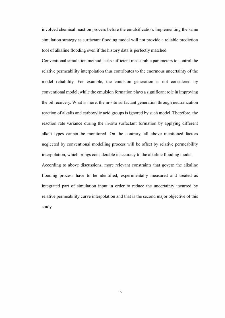
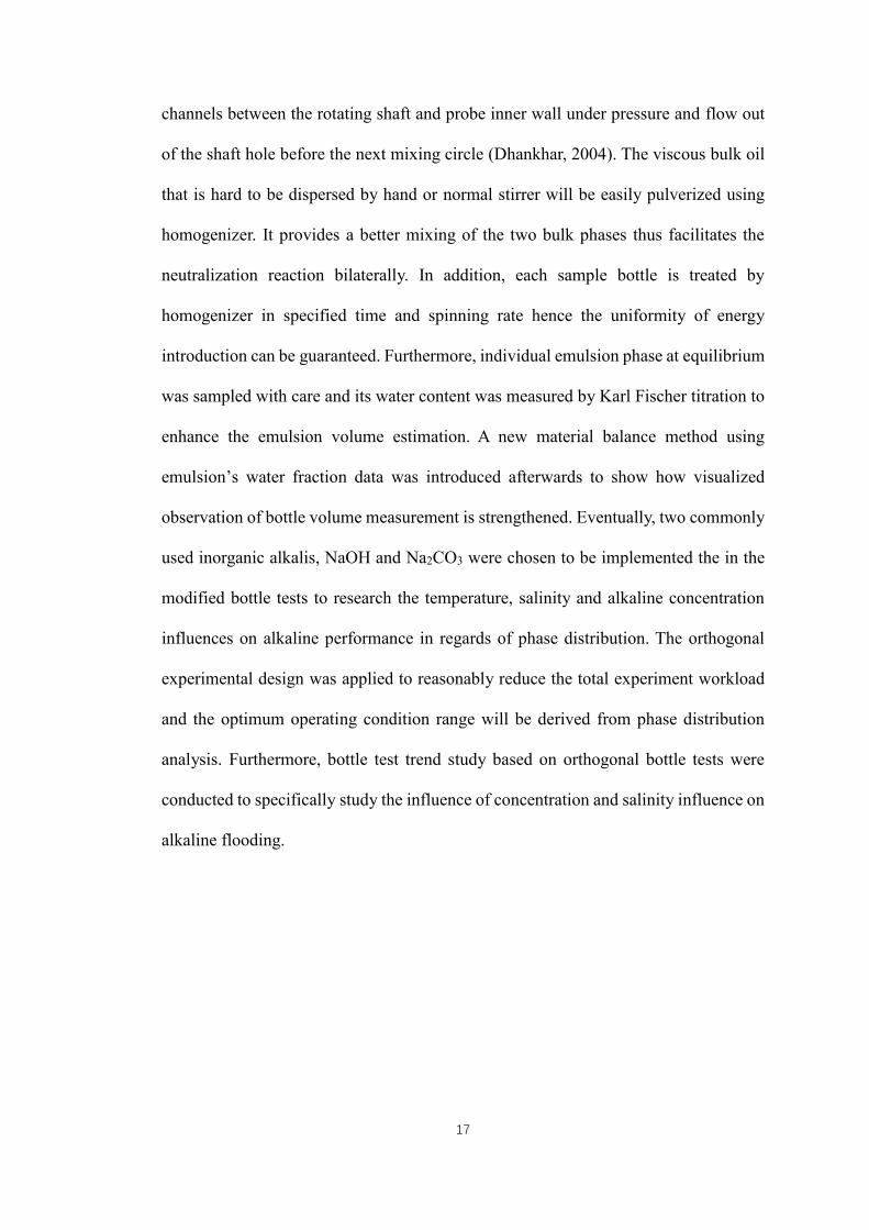
channels between the rotating shaft and probe inner wall under pressure and flow out
of the shaft hole before the next mixing circle (Dhankhar, 2004). The viscous bulk oil
that is hard to be dispersed by hand or normal stirrer will be easily pulverized using
homogenizer. It provides a better mixing of the two bulk phases thus facilitates the
neutralization reaction bilaterally. In addition, each sample bottle is treated by
homogenizer in specified time and spinning rate hence the uniformity of energy
introduction can be guaranteed. Furthermore, individual emulsion phase at equilibrium
was sampled with care and its water content was measured by Karl Fischer titration to
enhance the emulsion volume estimation. A new material balance method using
emulsion’s water fraction data was introduced afterwards to show how visualized
observation of bottle volume measurement is strengthened. Eventually, two commonly
used inorganic alkalis, NaOH and Na2CO3 were chosen to be implemented the in the
modified bottle tests to research the temperature, salinity and alkaline concentration
influences on alkaline performance in regards of phase distribution. The orthogonal
experimental design was applied to reasonably reduce the total experiment workload
and the optimum operating condition range will be derived from phase distribution
analysis. Furthermore, bottle test trend study based on orthogonal bottle tests were
conducted to specifically study the influence of concentration and salinity influence on
alkaline flooding.
18
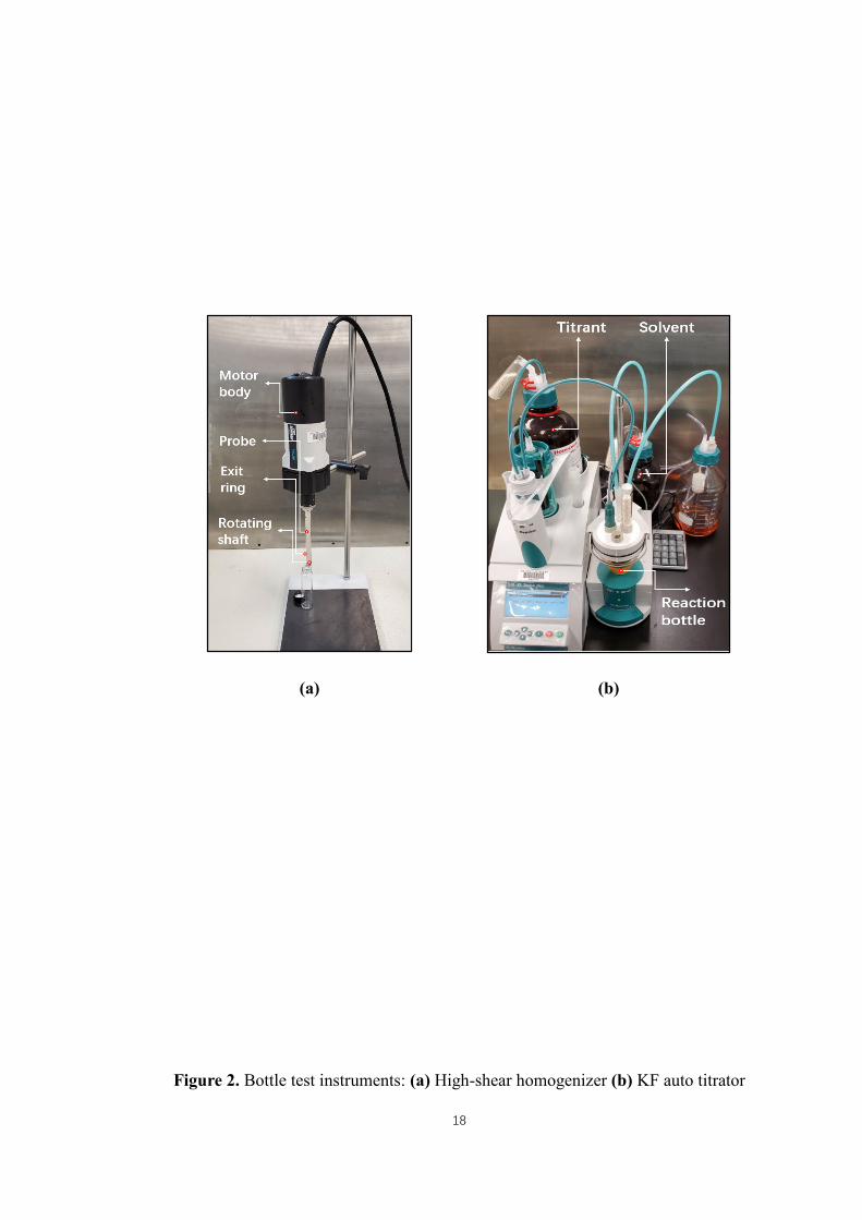
(a) (b)
Figure 2. Bottle test instruments: (a) High-shear homogenizer (b) KF auto titrator
19
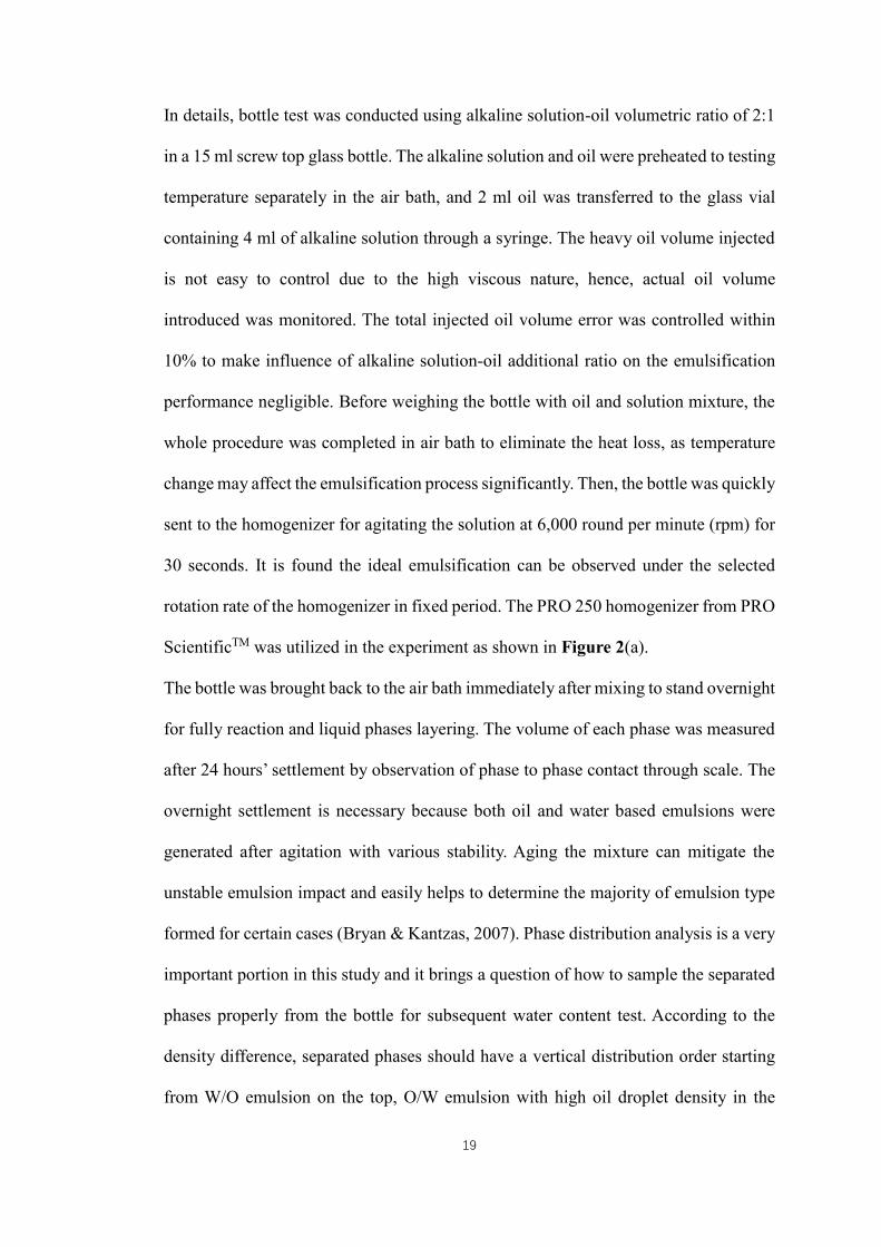
In details, bottle test was conducted using alkaline solution-oil volumetric ratio of 2:1
in a 15 ml screw top glass bottle. The alkaline solution and oil were preheated to testing
temperature separately in the air bath, and 2 ml oil was transferred to the glass vial
containing 4 ml of alkaline solution through a syringe. The heavy oil volume injected
is not easy to control due to the high viscous nature, hence, actual oil volume
introduced was monitored. The total injected oil volume error was controlled within
10% to make influence of alkaline solution-oil additional ratio on the emulsification
performance negligible. Before weighing the bottle with oil and solution mixture, the
whole procedure was completed in air bath to eliminate the heat loss, as temperature
change may affect the emulsification process significantly. Then, the bottle was quickly
sent to the homogenizer for agitating the solution at 6,000 round per minute (rpm) for
30 seconds. It is found the ideal emulsification can be observed under the selected
rotation rate of the homogenizer in fixed period. The PRO 250 homogenizer from PRO
ScientificTM was utilized in the experiment as shown in Figure 2(a).
The bottle was brought back to the air bath immediately after mixing to stand overnight
for fully reaction and liquid phases layering. The volume of each phase was measured
after 24 hours’ settlement by observation of phase to phase contact through scale. The
overnight settlement is necessary because both oil and water based emulsions were
generated after agitation with various stability. Aging the mixture can mitigate the
unstable emulsion impact and easily helps to determine the majority of emulsion type
formed for certain cases (Bryan & Kantzas, 2007). Phase distribution analysis is a very
important portion in this study and it brings a question of how to sample the separated
phases properly from the bottle for subsequent water content test. According to the
density difference, separated phases should have a vertical distribution order starting
from W/O emulsion on the top, O/W emulsion with high oil droplet density in the
20
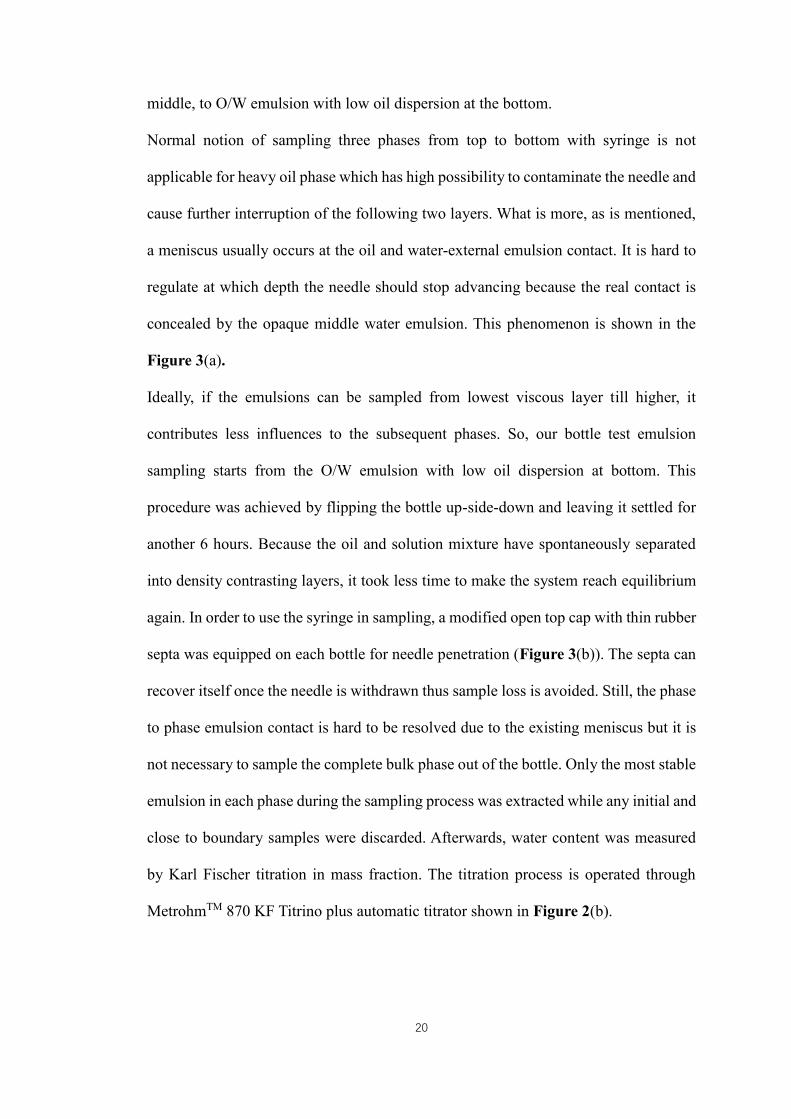
middle, to O/W emulsion with low oil dispersion at the bottom.
Normal notion of sampling three phases from top to bottom with syringe is not
applicable for heavy oil phase which has high possibility to contaminate the needle and
cause further interruption of the following two layers. What is more, as is mentioned,
a meniscus usually occurs at the oil and water-external emulsion contact. It is hard to
regulate at which depth the needle should stop advancing because the real contact is
concealed by the opaque middle water emulsion. This phenomenon is shown in the
Figure 3(a).
Ideally, if the emulsions can be sampled from lowest viscous layer till higher, it
contributes less influences to the subsequent phases. So, our bottle test emulsion
sampling starts from the O/W emulsion with low oil dispersion at bottom. This
procedure was achieved by flipping the bottle up-side-down and leaving it settled for
another 6 hours. Because the oil and solution mixture have spontaneously separated
into density contrasting layers, it took less time to make the system reach equilibrium
again. In order to use the syringe in sampling, a modified open top cap with thin rubber
septa was equipped on each bottle for needle penetration (Figure 3(b)). The septa can
recover itself once the needle is withdrawn thus sample loss is avoided. Still, the phase
to phase emulsion contact is hard to be resolved due to the existing meniscus but it is
not necessary to sample the complete bulk phase out of the bottle. Only the most stable
emulsion in each phase during the sampling process was extracted while any initial and
close to boundary samples were discarded. Afterwards, water content was measured
by Karl Fischer titration in mass fraction. The titration process is operated through
MetrohmTM 870 KF Titrino plus automatic titrator shown in Figure 2(b).

21
(a)
(b)
Figure 3. Glass bottle used in bottle test, (a) Unmeasurable top and middle phase
volume and (b) Glass bottle with open-top lid and rubber septa

22
In purpose of enhancing the phase volume observation, the material balance equation
is used to correct the visualization error mainly appears on oil-external emulsion and
middle water-external emulsion contact (see Figure 3(a)). The material balance
focused on the middle water-external emulsion volume calculation which can be
derived through two methods. The first method is called direct volume balance by
subtracting the top and bottom phases’ volume at equilibrium from initial total volume
ahead of mixing. It can be explained by the following equations:
Voi = (msao −msa)/ρoT [2.1]
Vmcalc1 = Voi + Vwi − Vo − Vw [2.2]
Another method takes advantage of the water content data of each phase and derives
the emulsion densities at equilibrium state in usage of rules of mixture, which is:
ρavg = V% × ρw + (100% − V%) × ρoT [2.3]
V% = 1/(1 + (ρw/ρoT) × (1/W%− 1)) [2.4]
It is assumed the mixture of the two immiscible fluids is in the form of one phase
becomes dispersed as droplets in the second phase thus generates one continuous phase
as emulsion (Chhabra; Richardson, 1999).
Since the original oil and alkaline solution volume are known, the middle emulsion
mass can also be calculated through deducting top and bottom emulsions’ mass from
the original total mass. Then, according to the middle emulsion density from water
content data, volume of middle emulsion is able to be calculated. The calculation can
be conducted by following equations:
mt = Voi × ρoT + Vwi ∗ ρw [2.5]
Vmcalc2 = (mt − Vo × ρavgo − Vw × ρavgw)/ρavgm [2.6]
Error% =Vmcalc2−Vmcalc1
Vmcalc2× 100% [2.7]
In a certain case, the middle emulsion generation is only trace amount which is

23
impossible to be sampled, its density is assumed to be the same as water conforming
to other successful sampling cases all having the middle emulsion density between 0.99
g/ mL to 0.996 g/ mL.
The two calculated middle emulsion volumes should be the same theoretically while
improper oil external emulsion volume observation results in large material balance
error. This material balance error can be mitigated by tuning the top phase volume
which is straightly related to middle emulsion volume. It is found that once the
appropriate tuning range is targeted, the material balance error can be significantly
reduced given correct tuning decision for majority of bottle tests.
Figure 4 provides a simplified work flow of the modified bottle test method to
summarize the above mentioned procedures in sequence.

24
Figure 4. Work flow of modified bottle test
25
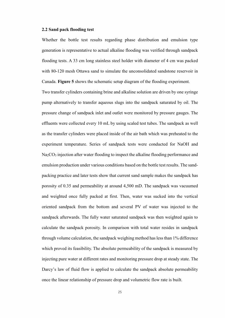
2.2 Sand pack flooding test
Whether the bottle test results regarding phase distribution and emulsion type
generation is representative to actual alkaline flooding was verified through sandpack
flooding tests. A 33 cm long stainless steel holder with diameter of 4 cm was packed
with 80-120 mesh Ottawa sand to simulate the unconsolidated sandstone reservoir in
Canada. Figure 5 shows the schematic setup diagram of the flooding experiment.
Two transfer cylinders containing brine and alkaline solution are driven by one syringe
pump alternatively to transfer aqueous slugs into the sandpack saturated by oil. The
pressure change of sandpack inlet and outlet were monitored by pressure gauges. The
effluents were collected every 10 mL by using scaled test tubes. The sandpack as well
as the transfer cylinders were placed inside of the air bath which was preheated to the
experiment temperature. Series of sandpack tests were conducted for NaOH and
Na2CO3 injection after water flooding to inspect the alkaline flooding performance and
emulsion production under various conditions based on the bottle test results. The sand-
packing practice and later tests show that current sand sample makes the sandpack has
porosity of 0.35 and permeability at around 4,500 mD. The sandpack was vacuumed
and weighted once fully packed at first. Then, water was sucked into the vertical
oriented sandpack from the bottom and several PV of water was injected to the
sandpack afterwards. The fully water saturated sandpack was then weighted again to
calculate the sandpack porosity. In comparison with total water resides in sandpack
through volume calculation, the sandpack weighing method has less than 1% difference
which proved its feasibility. The absolute permeability of the sandpack is measured by
injecting pure water at different rates and monitoring pressure drop at steady state. The
Darcy’s law of fluid flow is applied to calculate the sandpack absolute permeability
once the linear relationship of pressure drop and volumetric flow rate is built.

26
Figure 5. Schematic diagram of sandpack alkaline flooding test

27
The injection strategy of sandpack flooding tests is determined based on actual field
data. According to several pilot tests of NaOH flooding in the USA, the formations
with similar porosity and permeability to the sandpack were selected to investigate the
well injection rate. It is reported that it usually takes 15 years to inject 1 pore volume
(PV) of alkaline solution for a well with an average well injection rate of 1,000
barrel/day. Downscale the field injection to the sandpack model determines the
injection rate during the flooding test to be 1 ml/min. The calculation is shown as below:
1000 bbl/day = 110408 mL/min
sandpack injection rate = 110408 mL/min ×150 mL/q mL/min
15 × 365 × 24 × 60min
= q mL/min
Where 150 mL is the average sandpack pore volume and q is the initial injection rate
guess. Excel goal seek function was used to search for the q value that fulfills
110408mL
min×150 mL/x mL/min
15×365×24×60min− q
mL
min= 0 . It was found that when proposed
injection rate is 1.44 ml/min, the above calculation turns to be 0. Finally, 1 ml/min was
selected as a close value for the convenience of later data processing.
2.3 Chemical reaction rate test
2.3.1 Chemical reaction frequency factor theory
There are three reaction rates require to be determined as the initial input in the alkaline
flooding model. The first one is the saponification reaction between sodium hydroxide
and oleic acid components in the crude oil, which is followed by reaction 2 of
emulsification process. Another reaction is the depletion of sodium hydroxide (NaOH)
when it reacts with calcium chloride (CaCl2) which is assigned as reaction 3.
The reaction frequency factor ‘A’ or Arrhenius pre-exponential factor, has the unit of
dm3/mol-day or L/mol-day, determines the reaction rate constant ‘k’ at various
temperatures. This value in CMG is represented by keyword FREQFAC. It is an
28
important input which directly determines the alkali performance during the injection
process by quantifying the in-situ surfactant generation as well as the depletion of
NaOH concentration. The reaction frequency factor can be calculated based on reaction
rate constants with changing temperature. While reaction rate constant is the coefficient
of the relationship between the reaction rate and participating molecules or ions. Such
relation can be written as (Shao, et al, 2004):
v =dc
dt= k × (ci − c)
2 [2.8]
given the initial concentration of participating ion groups are the same and the second
order reaction is assumed. In order to measure k, the above equation is integrated into
the following equation as:
k =c
tci(ci−c) [2.9]
The reaction rate calculation focuses on the concentration change of the participating
ion groups, thus monitoring the ionic concentration change will be the key task in the
experiments. For reaction 3 regarding depletion of NaOH concentration when it is in
contact with CaCl2. The case is relatively simple because both CaCl2 and NaOH are in
aqueous phase. Since the precipitation reaction consumes [Ca2+] and [OH-]
simultaneously, either [Ca2+] ion can be measured by the ion selective electrode for
[Ca2+] or the system pH change can be tested using the InLab Expert Pro pH electrode.
Several preliminary tests have shown the reaction 3 rate is very fast so that ion selective
electrode which requires longer meter reading time was not selected. In this study, the
InLab Expert Pro pH electrode is used accompanying with the Mettler ToledoTM S220
SevenCompact pH/ion meter to accurately measure pH change in aqueous phase at
different temperatures. When it comes to reaction 1, similarly, determining of
saponification rate is based on system [OH-] concentration and meanwhile the [OH-]
concentration has a direct relation to pH of the aqueous phase. As is known, the water

29
autoprotolysis constant Kw is equal to the product of temperature relating
concentrations of [H3O+] and [OH-] by water dissociation.
So, log[Kw] = log[H3O+] + log[OH−] [2.10]
pKw = −log [Kw] [2.11]
pH = −log [H3O+] [2.12]
pOH = −log [OH−] [2.13]
pKw = pH + pOH [2.14]
The Kw value changes with temperature thus the neutral pH deviates from 7 more or
less at different temperature conditions. This is a very important parameter which
cannot be ignored because it directly determines the pH criterion. Later calculation
regarding Kw was based on the experiment temperature so pKw (pKw = 14 @ room
temperature) is not a fixed value.
Recall k =c
tci(ci−c) , the ci-c represents the NaOH molar depletion same as [OH−] .
Where [OH−] = 10(pH−pKw). Rearrange the equation gives:
(ci − 10(pH−pKw)) = kci × (t × 10
(pH−pKw)) [2.15]
So, by measuring the aqueous phase pH change along with time, above equation can
be plotted with ratio of (ci − 10(pH−pKw)) to (t × 10(pH−pKw)). Thus, the kci value
is able to be derived as the slope of the plot and the reaction rate can be further
calculated. The CMG simulator considers the temperature dependence of reaction rate
in form of Arrhenius equation. Therefore, reaction rate of the saponification reaction
was measured at different temperatures to derive the activation energy and Arrhenius
constant of the reaction. The Arrhenius equation is shown as (Arrhenius, 1889):
k = Ae−EaRT [2.16]
where Ea is the activation energy with the same unit as RT. Rearrange the equation and
30
take natural logarithm gives:
ln k = ln A +−Ea
RT [2.17]
and it is further derived to be:
ln k = (−Ea
R)(1
T) + ln A [2.18]
as a linear relation between temperature reciprocal and natural logarithm reaction
frequency factor. The slope of the linear relation is −Ea
R and reaction rate is calculated
once the Arrhenius constant (FREQFAC) and activation energy (Ea) data are input into
the CMG simulator.
On the other hand, the reaction 2 which represents the emulsification process regarding
oil/water dispersion has unknown reaction frequency factor and it is also hard to be
measured. This is because the emulsification process is not exactly chemistry
dominated but physically controlled by interfacial tension and charge power of
dispersed particles. However, the stoichiometry of the reaction equation can still be
derived based on the preliminary emulsification bottle test with the reagents and
production molecular weight.
2.3.2 Experiment design of reaction rate test
It was designed to preheat the two reagents (NaOH and oil) separately in the air bath
to targeted temperature at the first stage. The measurement of pH changes along with
chemical reactions was conducted at different temperatures. So, a beaker containing
mixed preheated chemical substances would be immersed into a water bath to maintain
temperature during the test. The water bath was covered by several circular covers
allowing electrode insertion into the beaker. The beaker itself was sealed by a rubber
stopper to prevent possible mass loss from the water vaporization. Because the pH
electrode tip can only measure one point of the aqueous phase, agitation of aqueous
phase is necessary to make the measured point representative. The magnetic stirrer bar
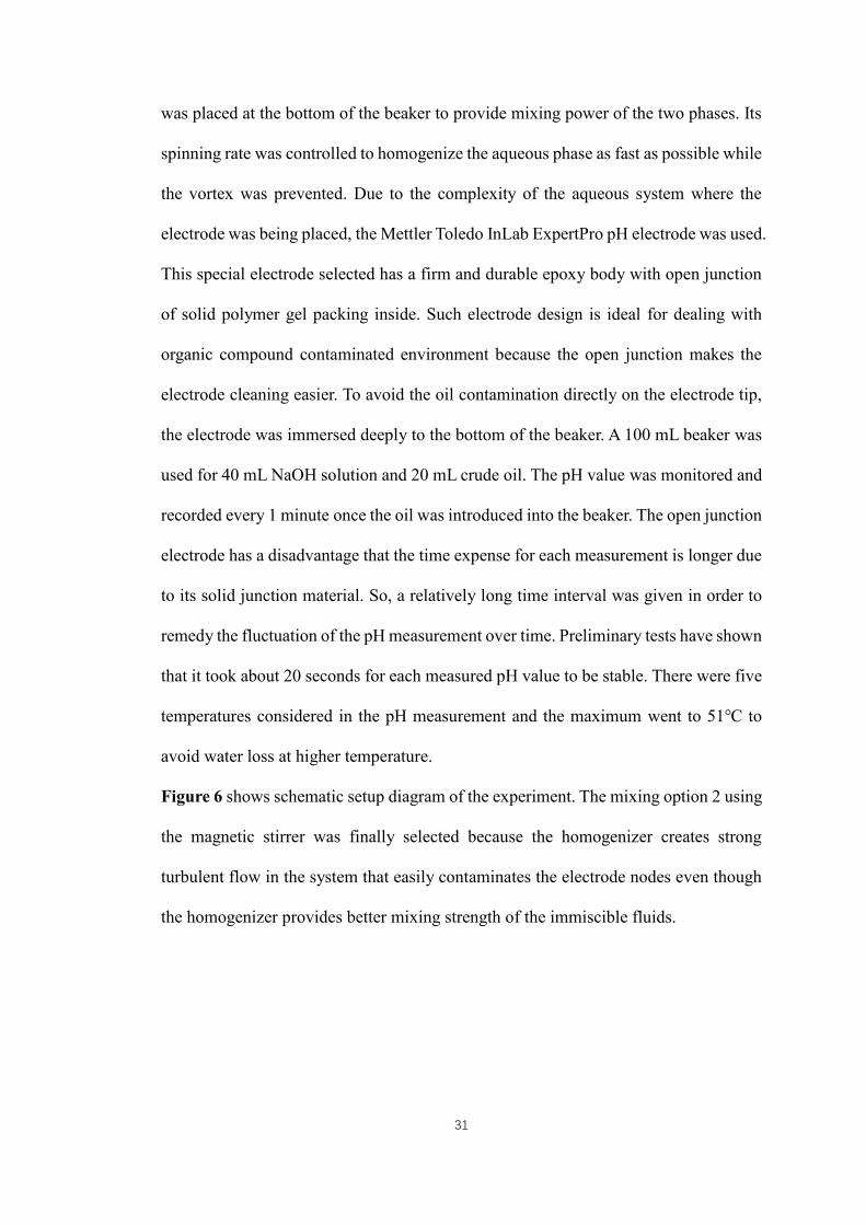
31
was placed at the bottom of the beaker to provide mixing power of the two phases. Its
spinning rate was controlled to homogenize the aqueous phase as fast as possible while
the vortex was prevented. Due to the complexity of the aqueous system where the
electrode was being placed, the Mettler Toledo InLab ExpertPro pH electrode was used.
This special electrode selected has a firm and durable epoxy body with open junction
of solid polymer gel packing inside. Such electrode design is ideal for dealing with
organic compound contaminated environment because the open junction makes the
electrode cleaning easier. To avoid the oil contamination directly on the electrode tip,
the electrode was immersed deeply to the bottom of the beaker. A 100 mL beaker was
used for 40 mL NaOH solution and 20 mL crude oil. The pH value was monitored and
recorded every 1 minute once the oil was introduced into the beaker. The open junction
electrode has a disadvantage that the time expense for each measurement is longer due
to its solid junction material. So, a relatively long time interval was given in order to
remedy the fluctuation of the pH measurement over time. Preliminary tests have shown
that it took about 20 seconds for each measured pH value to be stable. There were five
temperatures considered in the pH measurement and the maximum went to 51℃ to
avoid water loss at higher temperature.
Figure 6 shows schematic setup diagram of the experiment. The mixing option 2 using
the magnetic stirrer was finally selected because the homogenizer creates strong
turbulent flow in the system that easily contaminates the electrode nodes even though
the homogenizer provides better mixing strength of the immiscible fluids.

32
Figure 6. Reaction rate test setup
33
CHAPTER 3: Experiment works and results
In the previous chapter, the fundamentals of major experimental designs and theories
that fulfill the research objectives have been introduced. In this chapter, many detailed
fluid analysis procedures and results which are also vital as solid inputs for modified
bottle test or numerical simulation will be further discussed.
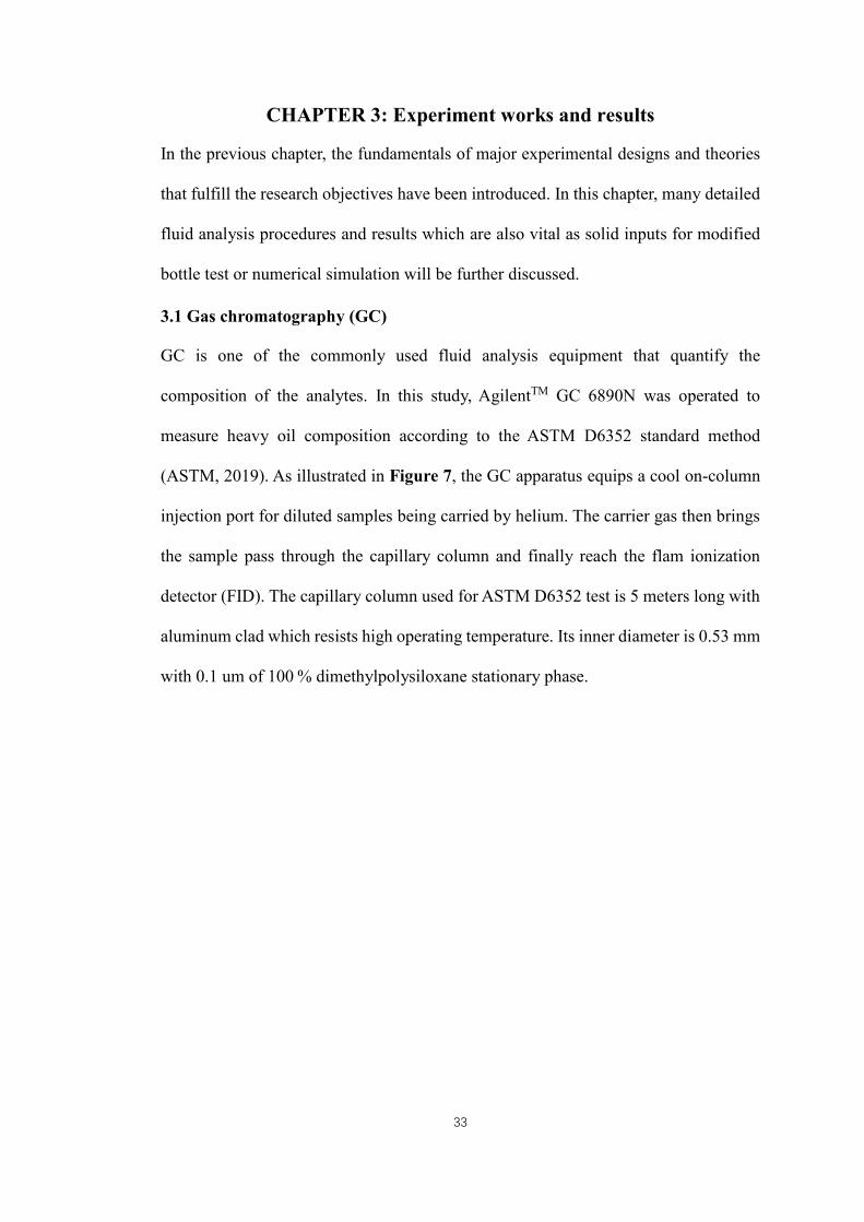
3.1 Gas chromatography (GC)
GC is one of the commonly used fluid analysis equipment that quantify the
composition of the analytes. In this study, AgilentTM GC 6890N was operated to
measure heavy oil composition according to the ASTM D6352 standard method
(ASTM, 2019). As illustrated in Figure 7, the GC apparatus equips a cool on-column
injection port for diluted samples being carried by helium. The carrier gas then brings
the sample pass through the capillary column and finally reach the flam ionization
detector (FID). The capillary column used for ASTM D6352 test is 5 meters long with
aluminum clad which resists high operating temperature. Its inner diameter is 0.53 mm
with 0.1 um of 100 % dimethylpolysiloxane stationary phase.
34
Figure 7. Schematic diagram of Agilent 6890N GC

35
The principle of the GC to measure composition of oil analyte is mainly relies on
components retention in the capillary tube. Heavy oil is composed by hundreds and
thousands of hydrocarbon substances with various molecular weights, boiling points
and structures. When oil sample is injected into the cool on-column inlet, the inlet
chamber temperature which is pre-programmed to rise with time will separate the light
and heavy substances in sequence according to their boiling points. The capillary
column coated with dimethylpolysiloxane is a non-polar adsorption surface with high
porosity. When separated hydrocarbons enter into the column, light molecules adsorb
and desorb from the coating faster than following heavier molecules. So, the long
capillary column further separates the hydrocarbon components along the carrier gas
flow path thus the separated components will arrive the detector in orders based on
their retention time throughout the capillary column. The FID detector is able to detect
the ion concentration formed during the combustion of hydrocarbons in the hydrogen
flame. This type of detector is mass sensitive due to its measuring mechanism, so,
heavy oil has to be diluted with carbon disulfide before being injected into the sample
inlet. The output chromatograph shows the ion concentration signal versus retention
time. Therefore, the mass fraction of each type of components can be determined from
the chromatograph by analyzing the signal strength at certain retention times.
The general GC compositional analysis of heavy oil sample by simulated distillation is
provided in the following section along with final results. The oil sample was weighed
and diluted into carbon disulfide as 1 wt.% solution. The cool on-column inlet
temperature was set in oven track mode whose initial temperature is 50 ℃ with 0 min
initial hold time. The oven temperature was increased by 10 ℃/min until 430 ℃ and
hold for 6 minutes when maximum temperature was reached. The FID was ignited
using hydrogen by feeding pure air at 450 ℃. Carrier gas flow rate was at 18 mL/min.

36
The column was baked at 250 ℃ for 2 hours and it is later purged with helium gas
overnight. Afterwards, the mixture of ASTM D2887 and Polywax 655 calibration mix
which includes the carbon number range from C5 to C44 and C40 to C110 respectively
was firstly measured in order to determine the specific retention time of each type of
the substance. Before that, C13, C14 and C15 FID performance calibration mixture has
been injected as internal standard to locate the C14 retention time. Based on the known
C14 retention time, other standard component location can be traced back and forth to
finish the calibration mix chromatograph analysis as shown in Figure 8(a).
Comparing the measured retention time of C44 and C90 to the reference chromatograph
from ASTM 6352 method in Figure 8(b), it is found the retention time error is less
than 60 seconds which means the repeatability of such method on Agilent 6890N GC
is satisfying.

37
(a)
(b)
Figure 8. Standard mix chromatographs (a) 6890N GC measured and (b) reference
chromatograph provided by Agilent

38
Figure 9. Heavy oil sample chromatograph edited by Agilent ChemStation

39
Then, a blank run is conducted before the sample run using the same standard method
to calibrate the base line. A complete composition test requires three chromatographs
including blank run, standard run and sample run processed by Agilent ChemStation
to subtract the blank chromatograph from the analyte chromatographs to reduce the
background noise. The final heavy oil sample chromatograph processed by Agilent
ChemStation is provided in the Figure 9.
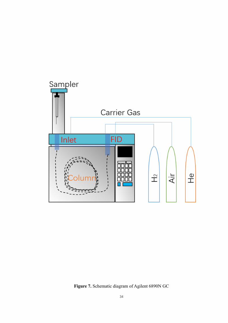
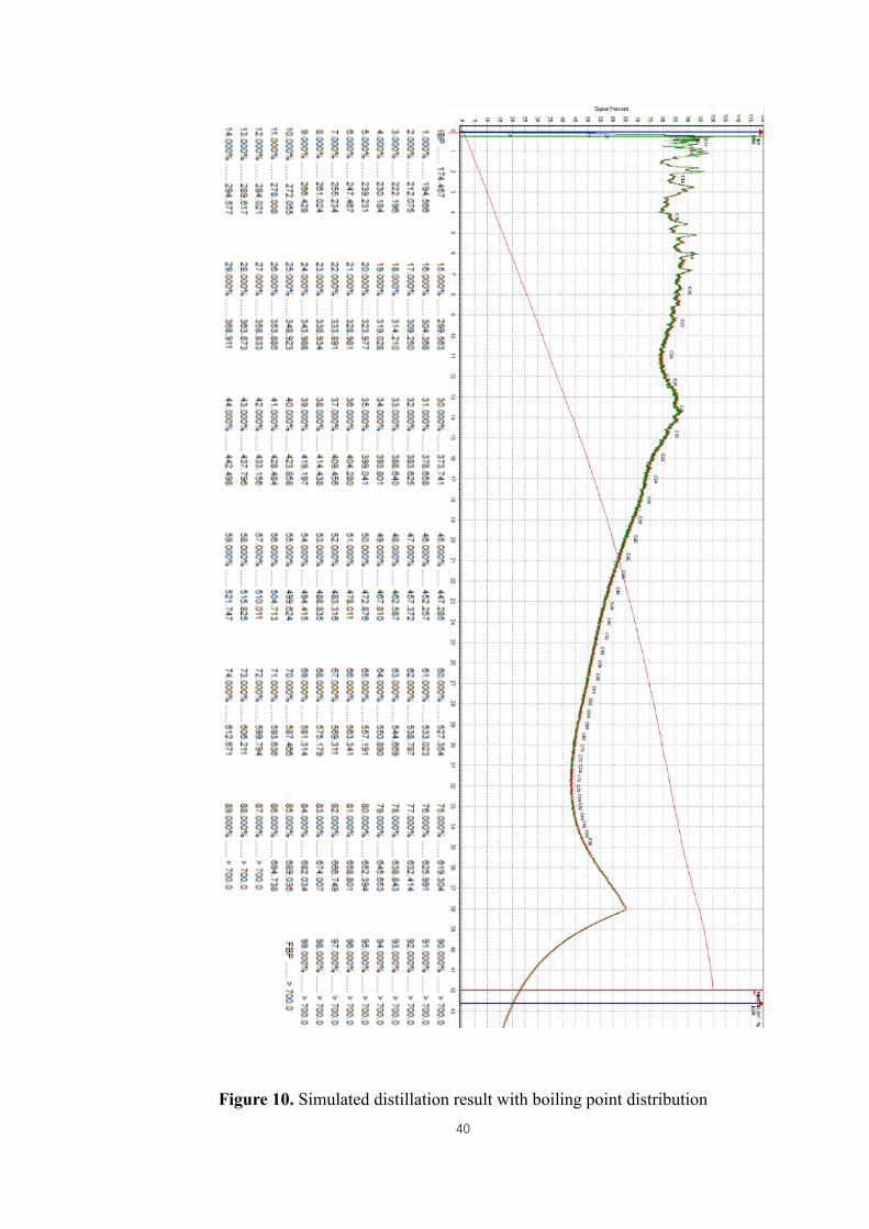
The processed chromatograph was later input into the EvantageTM SimDist software to
conduct simulated distillation. Figure 10 shows the location of each carbon number
components group on the chromatograph as well as the boiling point distribution
according to weight fraction.
Through which the composition of oil is able to be further derived based on provided
boiling point distribution. The boiling point interpolation was conducted automatically
according to the normal alkanes’ boiling points from ASTM6352 method by Matlab
through coding which is provided in Appendix A.
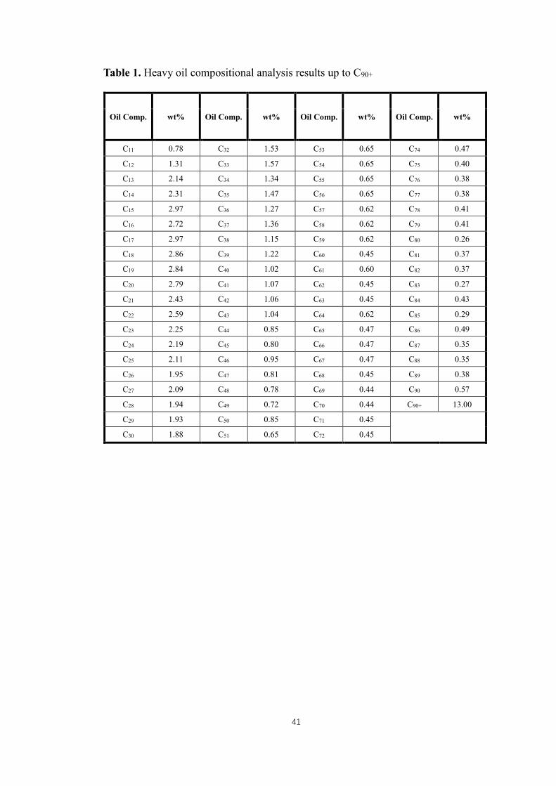
The measured oil composition up to C90+ is shown in Table 1, which was later used for
building the oil model by CMG WinPropTM.
40
Figure 10. Simulated distillation result with boiling point distribution
41
Table 1. Heavy oil compositional analysis results up to C90+
Oil Comp. wt% Oil Comp. wt% Oil Comp. wt% Oil Comp. wt%
C11 0.78 C32 1.53 C53 0.65 C74 0.47
C12 1.31 C33 1.57 C54 0.65 C75 0.40
C13 2.14 C34 1.34 C55 0.65 C76 0.38
C14 2.31 C35 1.47 C56 0.65 C77 0.38
C15 2.97 C36 1.27 C57 0.62 C78 0.41
C16 2.72 C37 1.36 C58 0.62 C79 0.41
C17 2.97 C38 1.15 C59 0.62 C80 0.26
C18 2.86 C39 1.22 C60 0.45 C81 0.37
C19 2.84 C40 1.02 C61 0.60 C82 0.37
C20 2.79 C41 1.07 C62 0.45 C83 0.27
C21 2.43 C42 1.06 C63 0.45 C84 0.43
C22 2.59 C43 1.04 C64 0.62 C85 0.29
C23 2.25 C44 0.85 C65 0.47 C86 0.49
C24 2.19 C45 0.80 C66 0.47 C87 0.35
C25 2.11 C46 0.95 C67 0.47 C88 0.35
C26 1.95 C47 0.81 C68 0.45 C89 0.38
C27 2.09 C48 0.78 C69 0.44 C90 0.57
C28 1.94 C49 0.72 C70 0.44 C90+ 13.00
C29 1.93 C50 0.85 C71 0.45
C30 1.88 C51 0.65 C72 0.45

42
3.2 Fourier-transform infrared spectroscopy (FTIR)
The FTIR test is conducted to explain the neutralization reaction of the acidic oils and
alkali in the preliminary study. It is known that different chemical bond of the
molecules contributes to various IR absorbance due to the bond vibration. The FTIR
utilizes the different infrared absorption abilities of functional groups of a sample to
determine certain molecular structures. For heavy oil case in reaction with alkalis,
carboxylic acid groups on asphaltenes is the major part that interact with the [OH-]
group to be depleted. Monitoring the carboxylic acid group quantity of the asphaltenes
is capable of providing the evidence of its neutralization reaction with alkalis. However,
the typical spectrum peak representing carboxylic acid groups was concealed by other
functional groups due to the complexity of the heavy oil components. So, the
asphaltenes have to be extracted from the oil sample before conducting the FTIR
measurement. In this study, the oil sample reacted with alkaline solution at certain
concentration after bottle test was collected in the flask. The oil surface was washed by
deionized water to remove the extra alkalis and left to be dried. Then, pentane was
introduced into the flask volumetrically 40 times more than oil to dilute the oil sample.
The asphaltenes have extremely low solubility to pentane so it was separated out of the
crude oil gradually with oscillation. The flask was then heated up to 50 ℃ to be hot
filtrated by Buchner funnel system in order to make the wax and resins re-dissolve into
the solution at high temperature. The asphaltenes cake therefore accumulated on the
filter paper and it was being washed by pentane to remove oil residuals. Finally, the
asphaltenes cake was left overnight in the fume hood to be dried.

43
Afterwards, the asphaltenes sample is processed by Perkin ElmerTM UATR polarizer
accessary with Spectrum One FTIR to derive the spectrum. It is clear to see from
Figure 11 that the alkanes’ C-H bound peaks located at 2,840 s-1 to 3,000 s-1 of the
three spectrums are overlapped with each other which means the type and quantity of
alkanes in the oil composition does not change after the reaction. On the other hand,
the 3,200-3,550 s-1 peak which represents O-H group for oil after alkaline reaction
diverges a lot. Because the O-H group embodies the alkaline level of the oil, original
oil has the lowest absorbance at this wavelength range while the oil mixed with alkaline
solution has higher absorbance. This peak height increases when oil reacts with higher
concentration of alkaline solution. The peaks within 1,395 s-1 to 1,440 s-1 stands for the
carboxylic acid group’s O-H bending of the asphaltenes of crude oil. Besides, the peak
located at 1,650 s-1 is interpreted as carboxylic acid group’s C=O stretching. According
to the spectrums, the asphaltenes from original oil has the highest peaks in wavelength
between 1,395 s-1 to1,440 s-1 indicating the strongest O-H vibration of carboxylic acid
groups. After the reaction with alkaline solution, the number of O-H bonds on
carboxylic acids reduces. According to the two cases with alkaline reaction, their O-H
bending absorbance are lower than the original oil. Nevertheless, the peak at 1,650 s-1
wavelength representing C=O stretching shows the opposite order on the other hand.
The asphaltenes of original oil shows a short and sharp peak in this case; however,
asphaltenes of oil sample with alkaline reaction are observed to show higher and
broader peaks. This phenomenon illustrates the saponification reaction mechanism of
oil and alkaline solution that generates carboxylate groups [RCOO-].

44
Original oil
Oil reacted with 0.002 mol/L Na2CO3 solution
Oil reacted with 0.004 mol/L Na2CO3 solution
Figure 11. FTIR spectrum of pentane extracted asphaltenes from crude oil and oil
after neutralization reaction

45
Once alkaline solution is introduced into the oil, the dissociated [OH-] group reacts
with carboxylic acid group [-COOH] on asphaltenes of crude oil. This neutralization
reaction generates carboxylate salts [R-COONa] which functions as surfactants with
lipophilic asphaltenes end and hydrophilic carboxylate end. Once the hydrogen ion of
the carboxylic acid is replaced by sodium ion, the initial weak acids are turned into
salts with higher dissociation in the aqueous phase. The C=O bond in carboxylate
groups becomes stronger due to the loss of its originally conjugated O-H bond since
[Na+] ion is more active and dispersible. Therefore, the higher alkaline concentration
contributes to more carboxylate groups followed by lower alkaline concentration case
which can be traced by their peak height at 1,650 s-1 and 1,350-1,400 s-1. Last but not
least, it is found the pentane extracted asphaltenes content of the oil sample is around
14 wt% which is close to the data of SARA measurement by commercial lab.
46
3.3 Karl Fischer volumetric water content titrator
The water content of emulsions was measured through Karl Fischer (K-F) titration
method in this study. The K-F volumetric water content titrator is used because it is
suitable for wide range of water content measurement from 0 wt% to 100 wt% water
of the sample. The Coulometric titration is not selected because of its limited measuring
range even though it has better accuracy. The principle of K-F titration is based on an
oxidation reaction of iodine that consumes water. Basically, the sample is injected into
the reaction cell containing absolute solvent like ethanol. Then, titrant including iodine
will be introduced into the reaction cell to react with any possible water content brought
by the sample. The cell is monitored by a conductivity electrode to determine whether
the water is fully depleted. By quantifying the consumption of titrant the according
water depletion in the oxidation reaction can be calculated. Since the complete set of
K-F titrator is semi-sealed system and its pressure balance end is filled with desiccant,
the external water vapor invasion can be minimized. In Figure 12, it shows the
schematic diagram of the K-F titration system.
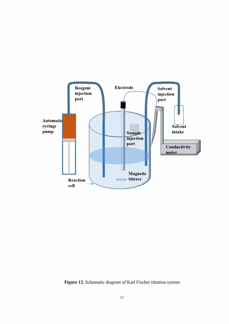
47
Figure 12. Schematic diagram of Karl Fischer titration system
48
For heavy oil samples, the oil is pre-diluted by carbon disulfide before being introduced
into the cell to reduce oil viscosity for smooth injection and reaction. Further
calculation is required to derive the correct water content for oil external emulsion. The
emulsion sample to be diluted and the carbon disulfide used were weighted in advance.
Afterwards, the diluted sample injection mass was calculated by measuring the syringe
weight before and after the injection. The actual water content of oil external emulsion
was calculated based on the following formula.
W%true = W% ∗mbo−mb
mboc−mb [3.1]
Calibration of the titrator is necessary before each measurement because the humid
atmosphere may slightly change the titrant performance in water consumption. The
Titrant 5 chemical was used based on the available sample volume in this study which
is capable to react with 0.02 mg water per gram of titrant. For medium to high water
content samples, the non-calibrated titrant will contribute to more than 50% of data
error. The measured emulsion water content data are shown in the modified screening
bottle test section along with further detailed emulsion distribution analysis.
3.4 pH/ion meter neutralization reaction rate test
The pH and ion meter is used for chemical reaction rate determination as well as the
effluents ion strength monitoring of the flooding tests. The meter used in the
experiment is manufactured by Mettler Toledo with compatible electrodes. The pH
measurement of the liquid sample is quite simple by inserting the electrode into the
sample and then read the displayed value. Because the pH value is sensitive to
temperature, a temperature sensor equipped in the electrode provides real time sample
temperature to calibrate the pH value simultaneously. The calibration is necessary for
the pH electrode to have reliable readings from the meter, thus, at least 3 different pH
standards with given pH values at various temperatures are required. In this study, the

49
pH standard with pH of 4, 7 and 10.1 at 20 ℃ were used and their pre-measured pH
values are within the temperature range from 20 to 50 ℃.
The chemical reaction rate test was conducted based on the experiment design in
Chapter 2.3.2. In total of 6 experiments have been completed to measure the
neutralization reaction rate of NaOH solution with heavy oil sample at the temperature
range between 27 and 51 ℃. Figure 13 and Figure 14 show the test results and some
conclusions can be drawn.

50
(a) pH decline curve with time at 27 ℃ (b) kci function curve at 27 ℃
(c) pH decline curve with time at 35 ℃ (d) kci function curve at 35 ℃
(e) pH decline curve with time at 39.5 ℃ (f) kci function curve at 39.5 ℃
Figure 13. Neutralization reaction tests at 27, 35 and 39.5 ℃

51
(a) pH decline curve with time at 42.5 ℃ (b) kci function curve at 42.5 ℃
(c) pH decline curve with time at 47 ℃ (d) kci function curve at 47 ℃
(e) pH decline curve with time at 51 ℃ (f) kci function curve at 51 ℃
(g) pH repeatability check at 35 ℃ (h) kci function repeatability check at 35 ℃
Figure 14. Neutralization reaction tests at 42.5, 47 and 51 ℃ with 35 ℃ repeatability
test
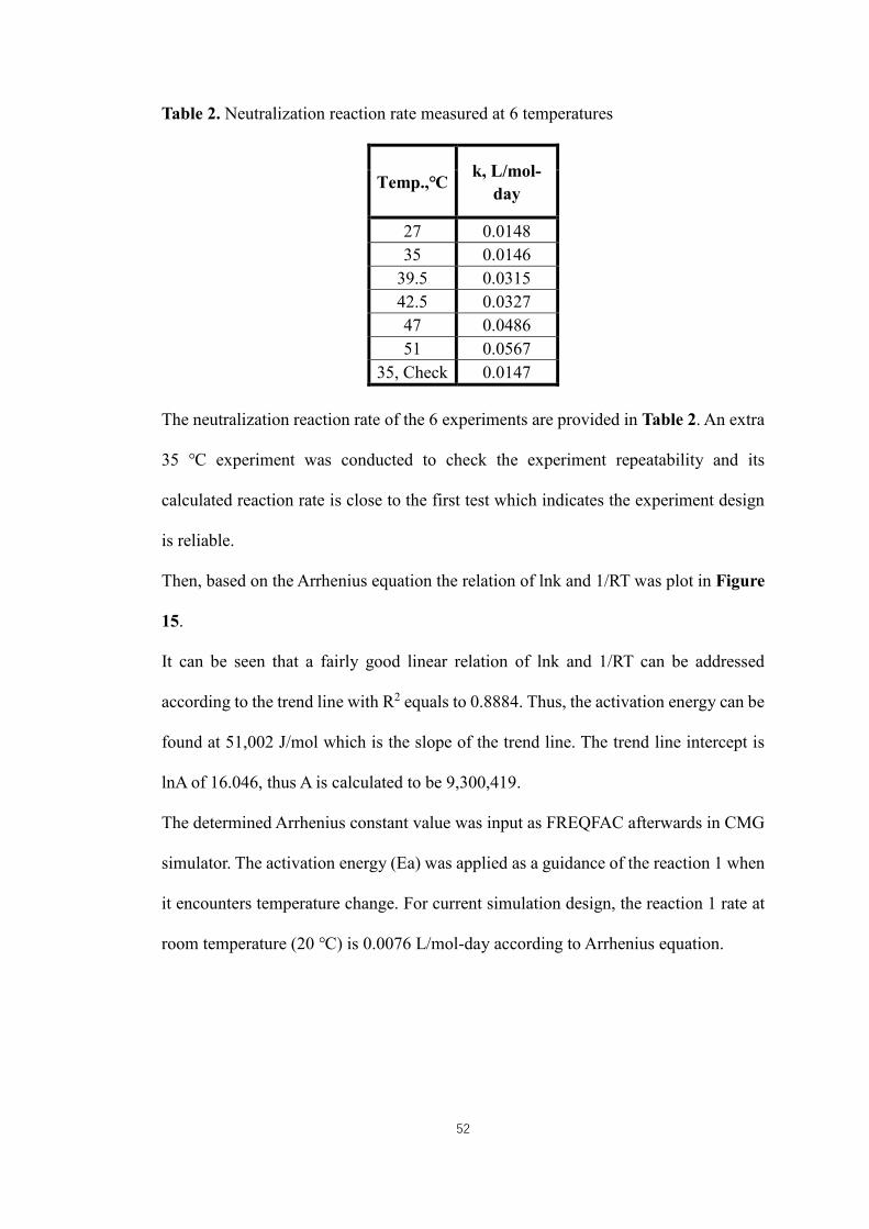
52
Table 2. Neutralization reaction rate measured at 6 temperatures
Temp.,℃ k, L/mol-
day
27 0.0148
35 0.0146
39.5 0.0315
42.5 0.0327
47 0.0486
51 0.0567
35, Check 0.0147
The neutralization reaction rate of the 6 experiments are provided in Table 2. An extra
35 ℃ experiment was conducted to check the experiment repeatability and its
calculated reaction rate is close to the first test which indicates the experiment design
is reliable.
Then, based on the Arrhenius equation the relation of lnk and 1/RT was plot in Figure
15.
It can be seen that a fairly good linear relation of lnk and 1/RT can be addressed
according to the trend line with R2 equals to 0.8884. Thus, the activation energy can be
found at 51,002 J/mol which is the slope of the trend line. The trend line intercept is
lnA of 16.046, thus A is calculated to be 9,300,419.
The determined Arrhenius constant value was input as FREQFAC afterwards in CMG
simulator. The activation energy (Ea) was applied as a guidance of the reaction 1 when
it encounters temperature change. For current simulation design, the reaction 1 rate at
room temperature (20 ℃) is 0.0076 L/mol-day according to Arrhenius equation.

53
Figure 15. Arrhenius equation plot

54
Through chemical reaction test of NaOH/oil, it can be clearly seen that the reaction
rate of neutralization reaction increases with temperature rise from Table 2. It is
theoretically reasonable because the dissociation of carboxylic acid is directly
proportional to temperature increase. Introducing extra energy into the reaction system
fulfills the requirement of hydrogen bond breaking from the molecule. The reaction
rate calculated from the tests all fall in the 0.01 L/mol-day magnitude thus the
significant change of reaction rate with temperature was not observed. This might be
due to the narrow temperature range selected during the test. Besides, the neutralization
reaction rate is also subjected to the mixing method during the measurement.
It has to be noted that, due to the experiment method limitation, the chemical reaction
rate measured from the aforementioned test is not necessary to represent the actual
neutralization reaction rate if only pure substances are involved. Carboxylic acid as
one of the target reagent is sourced from oleic phase. The high viscous oil used in the
test is immiscible to water thus mixing power as well as the oil viscosity play important
roles regarding carboxylic acid dissociation into the aqueous phase during the reaction.
Either increasing the temperature or amplifying the stirring power can improve the
contact of water and oil which facilitate the NaOH/oleic acid molecular collision
possibility. Therefore, the measured reaction rate from the aforementioned tests is not
purely chemical dominating since the neutralization reaction from common sense is
spontaneous and fast especially when it goes with strong alkalis.
As a matter of fact, the k value measured from the experiment is the reaction rate
specialized for reaction of immiscible phases which temperature, flow rate, viscosity
of the two phases are keys to the neutralization reaction rate in porous media. Thus, it
is still reasonable to use this set of reaction rate data in the CMG software.
During the pH measurement, it was found the displayed pH depletion turned unstable

55
after 3 to 5 minutes of the reaction. Analyzing the aqueous phase condition proved that
the oil dispersion in water occurred quickly and the emulsion had been generated
within the short reaction period under slow mixing rate. Dispersed oil contamination
on pH electrode tip makes it impossible to acquire further pH data and the emulsified
water also alters the conductivity of the system. So, the experiment was stopped once
the emulsion is formed and displayed pH value fluctuates. Nevertheless, since the
neutralization reaction rate is constant, as long as the initial pH reduction still follows
the depletion pattern, the pH value change at initial reaction stage is able to generate
sufficient data for the reaction rate model.
What is more, the reaction rate equation used at the first stage before integration has
the power-law value at 2 by assuming the chemical reaction to be second order.
v =dc
dt= k(ci − c)
2 [2.8]
The final model linearity (R2=0.8884) proved the initial assumption of neutralization
reaction order was correct.
Finally, the NaOH depletion due to the multivalent ions effect in aqueous phase is
considered in reaction 3. For reaction frequency factor and activation energy
determination, same pH measurement test will be conducted at different temperatures.
Since precipitation reaction is irreversible, the NaOH concentration is gradually
depleted thus contributes to decrease of pH value readings. In test 1, 0.01 mol/L CaCl2
solution was poured into the beaker containing 0.02 mol/L NaOH solution at 1:1
volume ratio at room temperature. Because the reagents were all in aqueous phases and
miscibility barrier did not exist, the reaction went at a very high rate comparing to the
previous neutralization reaction. The pH readings dropped almost suddenly and white
precipitation was observed right after the two solution contacted. So, the initial pH
value and the pH change after 1 second were recoded to calculate the rough reaction

56
rate of the precipitation reaction. Same experiment design was applied for test 2 except
the system temperature was increased to 40℃.
According to the slopes of the two tests shown in Figure 16, the reaction rate was
calculated to be 102.5 L/mol-day at 20 ℃ and 110.3 L/mol-day at 40 ℃. It is found
the precipitation reaction is an instant reaction and temperature independent thus its
reaction rate is way higher than what was measured in the water/oil neutralization
reaction. However, since the reaction 3 rate is too fast to record the accurate value
considering the inevitable human error during the test, further efforts need to be made
in order to acquire reliable reaction rate of the reaction 3.
Similar to the pH electrode, ion selective electrode was calibrated by three standards
at different ion concentrations before usage. The ionic concentration measurement data
will be shown in the numerical simulation of Chapter 5.

57
(a)
(b)
Figure 16. Precipitation reaction rate test at (a) 20 and (b) 40 ℃
58
3.5 Cone and plate viscometer and capillary method
The fluid viscosity measurement including crude oil and effluent emulsions was
conducted through cone plate viscometer or capillary method based on Hagen-
Poiseuille’s equation depending on the sample volume. The capillary method of fluid
viscosity measurement is widely suggested for its reliability and high result accuracy;
however, the sample quantity required by this method is large. So, it is not suitable for
emulsion viscosity measurement due to the limited emulsion quantity collected from
the sandpack flooding test. For small volume of liquid samples, the BrookfieldTM cone
and plate viscometer was used to measure the viscosity as substitution. The cone and
plate viscometer does not give the measured viscosity as accurate as capillary method
but it is more efficient to conduct series of measurements under various temperatures
within a short period. The capillary method based on Hagen-Poiseuille’s equation is
shown in the following equation.
μ =ΔP×π×Deff
Q×128×L [3.2]
The capillary method viscosity measurement experiment was conducted in an oven to
control temperature. Liquid sample was injected into the capillary tube from the
transfer cylinder at constant rate and the sample was discharged at the capillary output.
The pressure of the discharging end of the capillary tube is confined by a back pressure
regulator (BPR) and the pressure drop along the capillary tube can be calculated from
the pressure gauge readings. The length of the capillary tube used in experiment is 6 m
with inner effective diameter at 0.003134 m which is calibrated by viscous standard.
In this study, since the data of dead oil viscosity at different temperatures has been
provided by the commercial lab already, capillary method was conducted at 20 ℃ to
verify the existing viscosity data for improving the later oil model reliability. Test result
shows that pressure drop of the capillary ends was measured to be 3935.5 kPa at 0.2
59
mL/min. Thus, the dead oil viscosity at 20 ℃ calculated by Hagen-Poiseuille’s
equation was 23,866 cp. The capillary measured viscosity is close to the viscosity
measured by commercial lab (20,300 cp) with 14.7 % error. So, the oil properties
package provided are confident to be referred for building the CMG oil model.
The cone and plate viscometer was operated by routines to adjust the gap between the
cone and plate. 2 cm diameter spindle was placed under the spring rod for high viscous
fluid analysis. Then, 0.5 mL of emulsion collected from the NaOH flooding test was
transfer to the sample cup and water is circulated throughout the cup to maintain
operating temperature. The viscometer was firstly tested by viscous standard to check
its performance before conducting emulsion sample viscosity measurement and the test
results are shown in Table 3.
The performance tests showed the viscometer used in the test was able to provide
reliable sample viscosity readings since the measurement error of viscous standard is
less than 6 %. Then, emulsion sample was introduced into the sample holder to conduct
the measurement. The initial test set the spinning rate at 0.03 RPM. When meter
reading reached 160,000 cp, the viscometer spring torque has been overloaded.
Therefore, the second test reduced the spinning rate to 0.01 rpm. The meter reading
finally turned stable at 236,000 cp with 48.7 % spring torque. It can be seen that the
measured oil external emulsion viscosity at room temperature is more than ten times
higher than the dead oil viscosity. The emulsion viscosity increase was as expected
according to the viscosity model of the heavy oil emulsion system (Ersoy, et al., 2008).
The oil external emulsion viscosity should increase with its water content until the
inversion point is touched and the emulsion system turns into water external. The
measured emulsion viscosity was later used as input property for emulsion component
in CMG simulation.

60
Table 3. Viscosity measured by cone and plate viscometer
Sample standard
viscosity, cp readings, cp RPM Torque %
Standard 2908 2718 0.05 2.80
35510 34459 0.03 21.30
Emulsion - 160000 0.03 Overload
- 236000 0.01 48.70
61
3.6 Spinning drop tensiometer
Alkaline solution and oil IFT is an important index for bottle screening test and it is
also vital for numerical simulation which affects the capillary number of fluid flow
system. In this study, the TemcoTM spinning drop tensiometer was used to measure IFT.
Both oil and alkaline solution were preheated in the heating chamber at 70℃ to avoid
the viscosity barrel of heavy oil during the injection process. The prepared solution was
filled into a glass capillary tube at first. The capillary tube was then inserted into the
spindle of the preheated observation cell which drove the capillary tube spin along its
central axis at 2,000 rpm. Afterwards, a micro syringe containing oil sample was
inserted into the spinning capillary tube and one oil drop was introduced. The spinning
drop tensiometer focuses on the oil drop elongation in the capillary tube at certain
spinning rate. It is a continuous process and it stops when interfacial tension and
internal energy of the droplet reach equilibrium. The final drop shape is captured by a
high-speed camera and the captured image is processed by the Image J software to
measure its diameter and length. According to the elongation of droplet shape, the IFT
value was calculated based on the modified Vonnegut’s equation. The automatic
calculation was processed by Matlab through simple coding as shown in Appendix B.
Two alkaline solutions were applied in the test including NaOH and Na2CO3 to react
with heavy oil sample. Both effects of alkaline concentration change and salinity
change on water/oil IFT were studied according to the modified bottle test design.
Figure 17, Figure 18 stand for the 2 sets of IFT measurement conducted including
NaOH concentration and salinity effect tests. The Na2CO3 concentration and salinity
effect tests results are provided in Figure 19 and Figure 20.
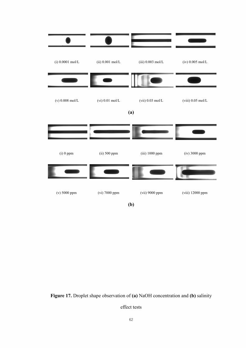
62
(i) 0.0001 mol/L (ii) 0.001 mol/L (iii) 0.003 mol/L (iv) 0.005 mol/L
(v) 0.008 mol/L (vi) 0.01 mol/L (vii) 0.03 mol/L (viii) 0.05 mol/L
(a)
(i) 0 ppm (ii) 500 ppm (iii) 1000 ppm (iv) 3000 ppm
(v) 5000 ppm (vi) 7000 ppm (vii) 9000 ppm (viii) 12000 ppm
(b)
Figure 17. Droplet shape observation of (a) NaOH concentration and (b) salinity
effect tests

63
(a)
(b)
Figure 18. IFT change with (a) NaOH concentration change and (b) salinity change
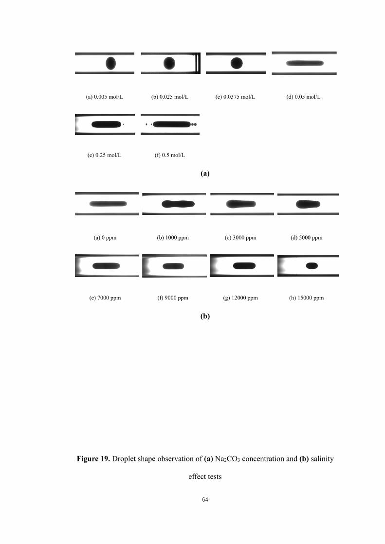
64
(a) 0.005 mol/L (b) 0.025 mol/L (c) 0.0375 mol/L (d) 0.05 mol/L
(e) 0.25 mol/L (f) 0.5 mol/L
(a)
(a) 0 ppm (b) 1000 ppm (c) 3000 ppm (d) 5000 ppm
(e) 7000 ppm (f) 9000 ppm (g) 12000 ppm (h) 15000 ppm
(b)
Figure 19. Droplet shape observation of (a) Na2CO3 concentration and (b) salinity
effect tests

65
(a)
(b)
Figure 20. IFT change with (a) Na2CO3 concentration change and (b) salinity change
66
According to the figures, sudden IFT curve drop is observed once alkaline solution is
introduced into the system. The IFT keeps decreasing until a certain concentration is
reached and further increase of concentration makes IFT slightly increase. The
optimum alkaline concentration can be determined based on where the lowest IFT is
located. For Na2CO3, the optimum alkaline concentration is 0.05 mol/L and it turns out
to be 0.03 mol/L for NaOH solution. On the other hand, the rise of system salinity
basically deals negative effect on the water/oil IFT for both NaOH and Na2CO3 cases
because the IFT increased couple of folds in high salinity system. The evaluation of
spinning drop IFT test will be discussed in Chapter 4.2 and comparison will be made
between the modified bottle test and the IFT test.

67
CHAPTER 4: Alkaline flooding driving mechanism investigation
In Chapter 2, the modified bottle test has been introduced to study the driving
mechanisms of the alkaline flooding through preparing and analyzing different
emulsions from the sample bottle. In this chapter, the modified bottle test has been
conducted using orthogonal experiment design following trend studies for two
different alkalis. The modified bottle test results are provided with detailed
examination of the dominating emulsion type formed under various environments.
Through which, the alkaline flooding mechanism is able to be predicted by the
modified bottle test.
4.1 Modified screening bottle test
Based on the methodology of modified bottle test, a series of bottle tests for two alkalis
with heavy oil under various conditions were conducted. Two inorganic alkalis
including NaOH and Na2CO3 were studied and the oil sample TAN is 2.1 mg KOH/g
oil. The oil viscosity is 20,300 cp at 20 ℃.
There were three main controlling factors studied for each alkali including alkaline
concentration, brine salinity and temperature. In order to determine the proper working
ranges for all three controlling factors, five levels were selected for each factor in a
relatively large scope, where alkaline concentration ranges from 0 ~ 0.5 mol/L, salinity
is within upper limit of 8,000 ppm and highest temperature goes to 70 ℃. The level
selection was determined by preliminary bottle test and it was also conformed to the
experimental condition restrictions. For instance, system temperature higher than 80 ℃
causes noticeable water vaporization thus results in potential weight loss. As the first
stage of screening bottle test, orthogonal design was conducted to reduce the attempted
125 bottle tests to 25 tests in total. The orthogonal experiment design is an experimental
strategy that is capable of taking individual parameters in estimation in a complex

68
system and obtaining optimum results (Athreya & Venkatesh, 2012). 25 combinations
of three controlling factors at certain levels were plugged in a refined L25(53)
orthogonal table for the purpose of evaluating the importance of each factor to alkaline
solution performance in emulsification with oil. The orthogonal design tables of NaOH
and Na2CO3 solutions are given in Table 4.

69
Table 4. Modified bottle test orthogonal experiment designs of two alkalis
(a) NaOH orthogonal experiment design
EXPs Temp, ℃ Salinity,
ppm
Aconc.,
mol/L
EXP1 20 0 0
EXP2 40 1000 0
EXP3 50 3000 0
EXP4 60 5000 0
EXP5 70 8000 0
EXP6 40 0 0.005
EXP7 50 1000 0.005
EXP8 60 3000 0.005
EXP9 70 5000 0.005
EXP10 20 8000 0.005
EXP11 50 0 0.01
EXP12 60 1000 0.01
EXP13 70 3000 0.01
EXP14 20 5000 0.01
EXP15 40 8000 0.01
EXP16 60 0 0.02
EXP17 70 1000 0.02
EXP18 20 3000 0.02
EXP19 40 5000 0.02
EXP20 50 8000 0.02
EXP21 70 0 0.05
EXP22 20 1000 0.05
EXP23 40 3000 0.05
EXP24 50 5000 0.05
EXP25 60 8000 0.05
(b) Na2CO3 orthogonal experiment design
EXPs Temp, ℃ Salinity,
ppm
Aconc.,
mol/L
EXP1 20 0 0
EXP2 40 1000 0
EXP3 50 3000 0
EXP4 60 5000 0
EXP5 70 8000 0
EXP6 40 0 0.005
EXP7 50 1000 0.005
EXP8 60 3000 0.005
EXP9 70 5000 0.005
EXP10 20 8000 0.005
EXP11 50 0 0.01
EXP12 60 1000 0.01
EXP13 70 3000 0.01
EXP14 20 5000 0.01
EXP15 40 8000 0.025
EXP16 60 0 0.025
EXP17 70 1000 0.025
EXP18 20 3000 0.025
EXP19 40 5000 0.04
EXP20 50 8000 0.04
EXP21 70 0 0.04
EXP22 20 1000 0.04
EXP23 40 3000 0.04
EXP24 50 5000 0.01
EXP25 60 8000 0.025
70
An evaluating index of the orthogonal experiment is necessary in ranking the alkaline
solution performance during the emulsification. In this case, the top and middle
emulsions volume fraction (V%m+o) among final phases at equilibrium is selected.
Based on previous alkaline flooding mechanism study, entrainment, entrapment and
wettability alteration phenomenon all facilitate the oil recovery (Johnson, 1976; Dong
et al., 2012). Thus, functioning emulsion type of alkaline flooding can be either O/W
emulsion or W/O emulsion. In consideration of alkaline flooding mechanisms, the
potential middle O/W emulsion and top W/O emulsion are key phases need to be
quantified. The oil dispersion in bottom water phase also occurred in most cases
coexisting with middle oil in water emulsion. However, a clear interface between the
bottom and middle phases can be observed. Since only trace amount of oil was
dispersed into the bottom phase due to the significantly low surfactant concentrations.
The bottom oil in water emulsion phase is treated irrelevant to effective emulsion
volume.
Despite that, the turbidity of the bottom water phase increases with larger volume of
middle phase. So, it still can be used as an indicator to illustrate the emulsification
quality to some extent. The middle phase is observable through bottle and water in oil
emulsion phase is determined if equipoised top phase volume is larger than original
introduced oil volume.
Table 5 and Table 6 exhibit the orthogonal bottle test emulsion volume fraction data
through material balance calibration.
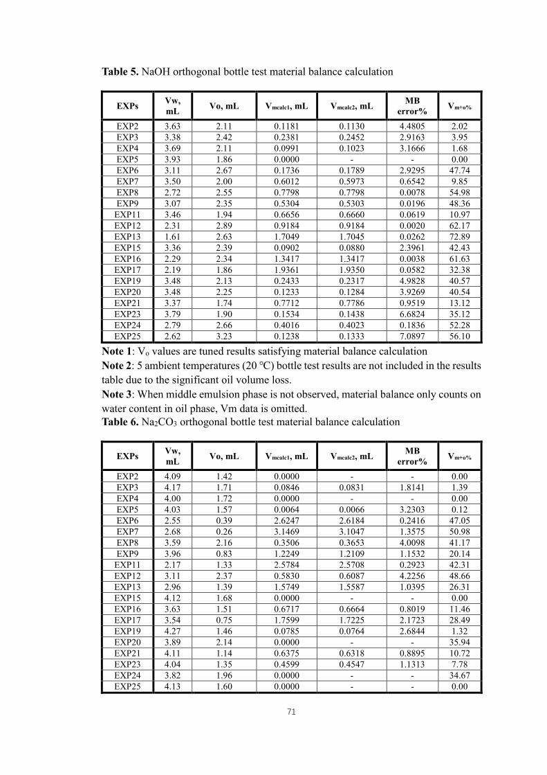
71
Table 5. NaOH orthogonal bottle test material balance calculation
EXPs Vw,
mL Vo, mL Vmcalc1, mL Vmcalc2, mL
MB
error% Vm+o%
EXP2 3.63 2.11 0.1181 0.1130 4.4805 2.02
EXP3 3.38 2.42 0.2381 0.2452 2.9163 3.95
EXP4 3.69 2.11 0.0991 0.1023 3.1666 1.68
EXP5 3.93 1.86 0.0000 - - 0.00
EXP6 3.11 2.67 0.1736 0.1789 2.9295 47.74
EXP7 3.50 2.00 0.6012 0.5973 0.6542 9.85
EXP8 2.72 2.55 0.7798 0.7798 0.0078 54.98
EXP9 3.07 2.35 0.5304 0.5303 0.0196 48.36
EXP11 3.46 1.94 0.6656 0.6660 0.0619 10.97
EXP12 2.31 2.89 0.9184 0.9184 0.0020 62.17
EXP13 1.61 2.63 1.7049 1.7045 0.0262 72.89
EXP15 3.36 2.39 0.0902 0.0880 2.3961 42.43
EXP16 2.29 2.34 1.3417 1.3417 0.0038 61.63
EXP17 2.19 1.86 1.9361 1.9350 0.0582 32.38
EXP19 3.48 2.13 0.2433 0.2317 4.9828 40.57
EXP20 3.48 2.25 0.1233 0.1284 3.9269 40.54
EXP21 3.37 1.74 0.7712 0.7786 0.9519 13.12
EXP23 3.79 1.90 0.1534 0.1438 6.6824 35.12
EXP24 2.79 2.66 0.4016 0.4023 0.1836 52.28
EXP25 2.62 3.23 0.1238 0.1333 7.0897 56.10
Note 1: Vo values are tuned results satisfying material balance calculation
Note 2: 5 ambient temperatures (20 ℃) bottle test results are not included in the results
table due to the significant oil volume loss.
Note 3: When middle emulsion phase is not observed, material balance only counts on
water content in oil phase, Vm data is omitted.
Table 6. Na2CO3 orthogonal bottle test material balance calculation
EXPs Vw,
mL Vo, mL Vmcalc1, mL Vmcalc2, mL
MB
error% Vm+o%
EXP2 4.09 1.42 0.0000 - - 0.00
EXP3 4.17 1.71 0.0846 0.0831 1.8141 1.39
EXP4 4.00 1.72 0.0000 - - 0.00
EXP5 4.03 1.57 0.0064 0.0066 3.2303 0.12
EXP6 2.55 0.39 2.6247 2.6184 0.2416 47.05
EXP7 2.68 0.26 3.1469 3.1047 1.3575 50.98
EXP8 3.59 2.16 0.3506 0.3653 4.0098 41.17
EXP9 3.96 0.83 1.2249 1.2109 1.1532 20.14
EXP11 2.17 1.33 2.5784 2.5708 0.2923 42.31
EXP12 3.11 2.37 0.5830 0.6087 4.2256 48.66
EXP13 2.96 1.39 1.5749 1.5587 1.0395 26.31
EXP15 4.12 1.68 0.0000 - - 0.00
EXP16 3.63 1.51 0.6717 0.6664 0.8019 11.46
EXP17 3.54 0.75 1.7599 1.7225 2.1723 28.49
EXP19 4.27 1.46 0.0785 0.0764 2.6844 1.32
EXP20 3.89 2.14 0.0000 - - 35.94
EXP21 4.11 1.14 0.6375 0.6318 0.8895 10.72
EXP23 4.04 1.35 0.4599 0.4547 1.1313 7.78
EXP24 3.82 1.96 0.0000 - - 34.67
EXP25 4.13 1.60 0.0000 - - 0.00
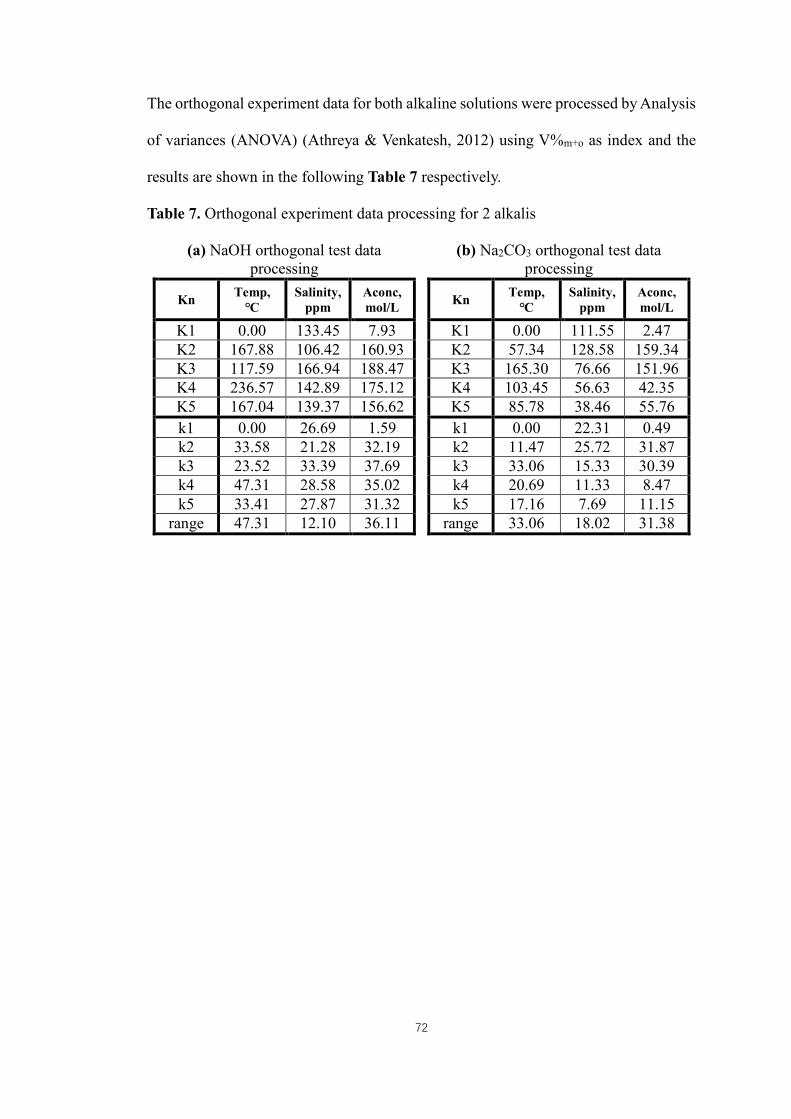
72
The orthogonal experiment data for both alkaline solutions were processed by Analysis
of variances (ANOVA) (Athreya & Venkatesh, 2012) using V%m+o as index and the
results are shown in the following Table 7 respectively.
Table 7. Orthogonal experiment data processing for 2 alkalis
(a) NaOH orthogonal test data
processing
Kn Temp,
℃
Salinity,
ppm
Aconc,
mol/L
K1 0.00 133.45 7.93
K2 167.88 106.42 160.93
K3 117.59 166.94 188.47
K4 236.57 142.89 175.12
K5 167.04 139.37 156.62
k1 0.00 26.69 1.59
k2 33.58 21.28 32.19
k3 23.52 33.39 37.69
k4 47.31 28.58 35.02
k5 33.41 27.87 31.32
range 47.31 12.10 36.11
(b) Na2CO3 orthogonal test data
processing
Kn Temp,
℃
Salinity,
ppm
Aconc,
mol/L
K1 0.00 111.55 2.47
K2 57.34 128.58 159.34
K3 165.30 76.66 151.96
K4 103.45 56.63 42.35
K5 85.78 38.46 55.76
k1 0.00 22.31 0.49
k2 11.47 25.72 31.87
k3 33.06 15.33 30.39
k4 20.69 11.33 8.47
k5 17.16 7.69 11.15
range 33.06 18.02 31.38
73
In the calculation, Kn of a factor represents the summation of estimating indices among
25 bottle tests at nth level and kn is the corresponding average. The range of a factor is
calculated by subtracting the lowest k value from the highest k value within five levels.
The factor range indicates the importance of a factor to the emulsification performance,
thus high range usually implies the compelling influence of a factor on emulsification
of alkaline solution and oil.
According to the bottle test results and phase distribution analysis, the overall
importance of alkaline concentration, brine salinity as well as temperature of NaOH
and Na2CO3 cases to emulsification quality were derived. First and foremost, the
ranking of the three factor ranges shows the same sequence for both alkaline solutions
which temperature change highly influences the amount of functional surfactants
generation followed by the alkaline concentration adjustment. It seems quite
reasonable because oil and water interference plays a critical role during the
emulsification process. High viscous oil under temperature scope between 20 and 40 ℃
will not be deformed easily due to its high molecular attraction that resists to flow
(Nagarajan, Dong, Mullins & Honarpour, 2012). Dispersion of oil droplets into water
requires significant shear rate to drag the particles off the main oil bulk phase at this
stage. Nevertheless, oil viscosity will substantially drop once the system temperature
increases which facilitates the oil and water mixing process. At temperature higher than
50 ℃, the oil viscosity is lower than 1,000 cp and it makes the oil easier to move and
be pulverized into small pieces. This phenomenon increases the contact possibility of
oil and alkaline solution and further promotes the neutralization reaction to generate
extra amount of in-situ surfactants. On the other hand, alkaline solution concentration
is related to the change of system [OH-] group concentration directly. Thus, it shares
similar weight of influence as temperature factor to the alkaline solution performance

74
in emulsification. The brine salinity is the least affecting factor going to alter the
emulsification. This is mainly because of the salinity range selected at 0 to 8,000 ppm
is lower than common reservoir brine salinity and only NaCl is considered in brine
synthesis. However, through salinity K value evaluation, brine with salinity lower than
5,000 ppm is somewhat preferred for higher volume of emulsion generation. The Kn
values of salinity factor have the highest magnitude in such range selected which
illustrates the optimum salinity point is within. Based on orthogonal bottle tests, the
optimum working conditions of temperature, salinity and alkaline concentration can be
roughly determined; however, due to the limited point selections and scattered
combinations of three controlling factors, it is inconvenient to wrap up a regular pattern
of phase distribution from orthogonal experiments. So, another two groups of bottle
test trend study were designed and conducted for NaOH and Na2CO3 to amplify the
emulsion phase distribution pattern with the change of controlling factors.
The trend study is mainly focused on the effects of alkaline concentration and salinity
change to phase distribution. Thus, the operating temperature is set at 70 ℃ to
ultimately facilitate the mixing and reaction according to the factor importance study
of both alkaline solutions. For each alkaline solution, alkaline concentration trend study
was conducted firstly and it keeps the salinity to be 0 ppm to exclude the salinity effect
thoroughly. Then, salinity trend test was performed afterwards at the optimum alkaline
concentration determined from the previous step. Table 8 shows the trend study bottle
test design for NaOH solution.
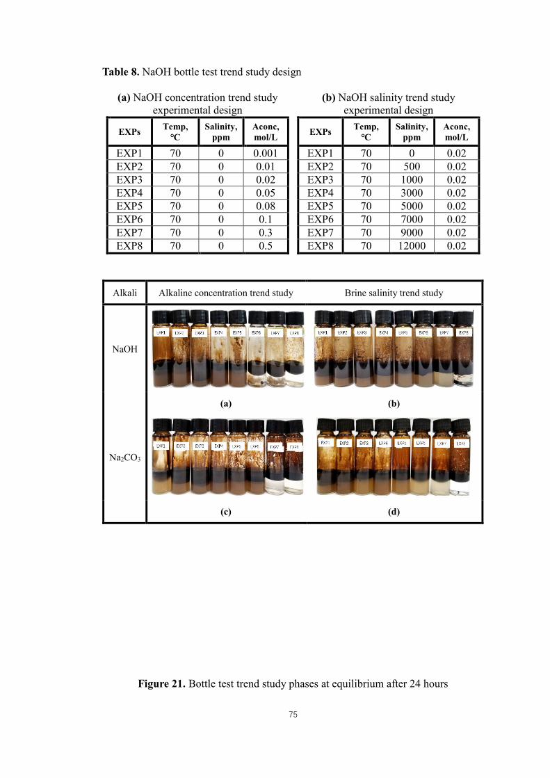
75
Table 8. NaOH bottle test trend study design
(a) NaOH concentration trend study
experimental design
EXPs Temp,
℃
Salinity,
ppm
Aconc,
mol/L
EXP1 70 0 0.001
EXP2 70 0 0.01
EXP3 70 0 0.02
EXP4 70 0 0.05
EXP5 70 0 0.08
EXP6 70 0 0.1
EXP7 70 0 0.3
EXP8 70 0 0.5
(b) NaOH salinity trend study
experimental design
EXPs Temp,
℃
Salinity,
ppm
Aconc,
mol/L
EXP1 70 0 0.02
EXP2 70 500 0.02
EXP3 70 1000 0.02
EXP4 70 3000 0.02
EXP5 70 5000 0.02
EXP6 70 7000 0.02
EXP7 70 9000 0.02
EXP8 70 12000 0.02
Alkali Alkaline concentration trend study Brine salinity trend study
NaOH
(a) (b)
Na2CO3
(c) (d)
Figure 21. Bottle test trend study phases at equilibrium after 24 hours
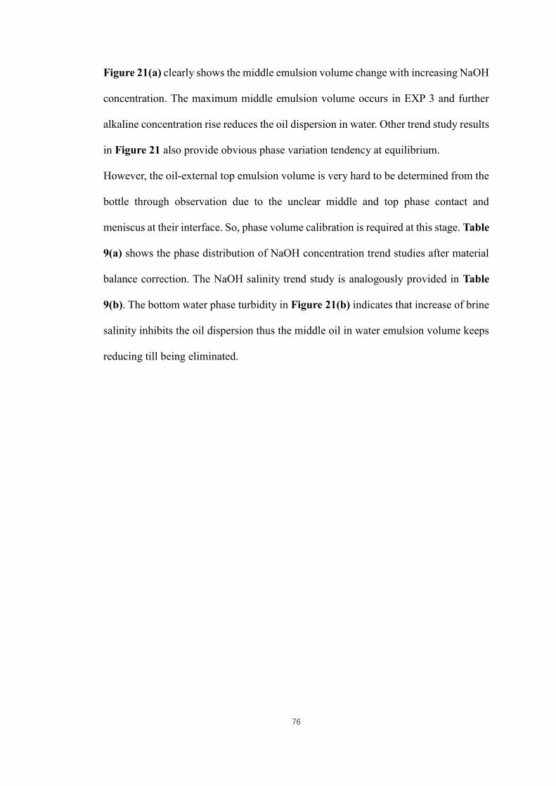
76
Figure 21(a) clearly shows the middle emulsion volume change with increasing NaOH
concentration. The maximum middle emulsion volume occurs in EXP 3 and further
alkaline concentration rise reduces the oil dispersion in water. Other trend study results
in Figure 21 also provide obvious phase variation tendency at equilibrium.
However, the oil-external top emulsion volume is very hard to be determined from the
bottle through observation due to the unclear middle and top phase contact and
meniscus at their interface. So, phase volume calibration is required at this stage. Table
9(a) shows the phase distribution of NaOH concentration trend studies after material
balance correction. The NaOH salinity trend study is analogously provided in Table
9(b). The bottom water phase turbidity in Figure 21(b) indicates that increase of brine
salinity inhibits the oil dispersion thus the middle oil in water emulsion volume keeps
reducing till being eliminated.
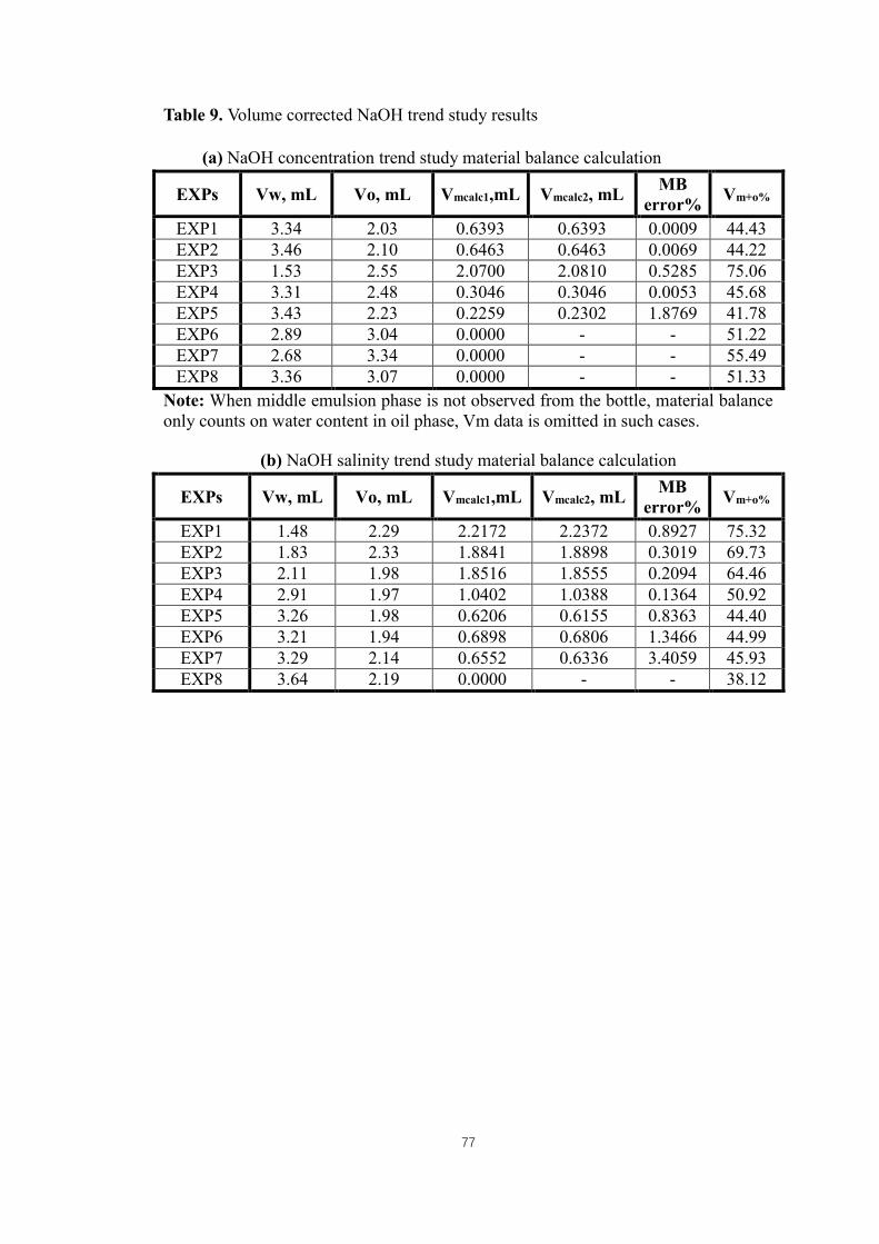
77
Table 9. Volume corrected NaOH trend study results
(a) NaOH concentration trend study material balance calculation
EXPs Vw, mL Vo, mL Vmcalc1,mL Vmcalc2, mL MB
error% Vm+o%
EXP1 3.34 2.03 0.6393 0.6393 0.0009 44.43
EXP2 3.46 2.10 0.6463 0.6463 0.0069 44.22
EXP3 1.53 2.55 2.0700 2.0810 0.5285 75.06
EXP4 3.31 2.48 0.3046 0.3046 0.0053 45.68
EXP5 3.43 2.23 0.2259 0.2302 1.8769 41.78
EXP6 2.89 3.04 0.0000 - - 51.22
EXP7 2.68 3.34 0.0000 - - 55.49
EXP8 3.36 3.07 0.0000 - - 51.33
Note: When middle emulsion phase is not observed from the bottle, material balance
only counts on water content in oil phase, Vm data is omitted in such cases.
(b) NaOH salinity trend study material balance calculation
EXPs Vw, mL Vo, mL Vmcalc1,mL Vmcalc2, mL MB
error% Vm+o%
EXP1 1.48 2.29 2.2172 2.2372 0.8927 75.32
EXP2 1.83 2.33 1.8841 1.8898 0.3019 69.73
EXP3 2.11 1.98 1.8516 1.8555 0.2094 64.46
EXP4 2.91 1.97 1.0402 1.0388 0.1364 50.92
EXP5 3.26 1.98 0.6206 0.6155 0.8363 44.40
EXP6 3.21 1.94 0.6898 0.6806 1.3466 44.99
EXP7 3.29 2.14 0.6552 0.6336 3.4059 45.93
EXP8 3.64 2.19 0.0000 - - 38.12
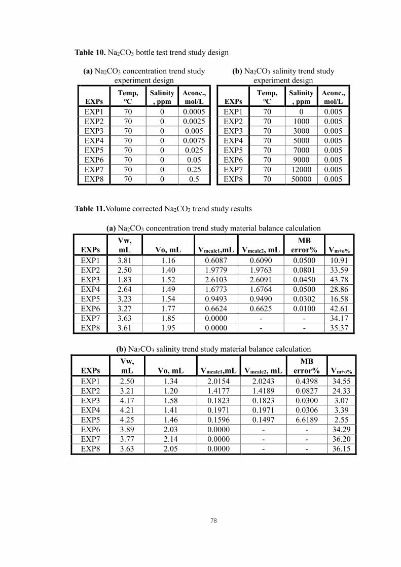
78
Table 10. Na2CO3 bottle test trend study design
(a) Na2CO3 concentration trend study
experiment design
EXPs
Temp,
℃
Salinity
, ppm
Aconc.,
mol/L
EXP1 70 0 0.0005
EXP2 70 0 0.0025
EXP3 70 0 0.005
EXP4 70 0 0.0075
EXP5 70 0 0.025
EXP6 70 0 0.05
EXP7 70 0 0.25
EXP8 70 0 0.5
(b) Na2CO3 salinity trend study
experiment design
EXPs
Temp,
℃
Salinity
, ppm
Aconc.,
mol/L
EXP1 70 0 0.005
EXP2 70 1000 0.005
EXP3 70 3000 0.005
EXP4 70 5000 0.005
EXP5 70 7000 0.005
EXP6 70 9000 0.005
EXP7 70 12000 0.005
EXP8 70 50000 0.005
Table 11.Volume corrected Na2CO3 trend study results
(a) Na2CO3 concentration trend study material balance calculation
EXPs
Vw,
mL Vo, mL Vmcalc1,mL Vmcalc2, mL
MB
error% Vm+o%
EXP1 3.81 1.16 0.6087 0.6090 0.0500 10.91
EXP2 2.50 1.40 1.9779 1.9763 0.0801 33.59
EXP3 1.83 1.52 2.6103 2.6091 0.0450 43.78
EXP4 2.64 1.49 1.6773 1.6764 0.0500 28.86
EXP5 3.23 1.54 0.9493 0.9490 0.0302 16.58
EXP6 3.27 1.77 0.6624 0.6625 0.0100 42.61
EXP7 3.63 1.85 0.0000 - - 34.17
EXP8 3.61 1.95 0.0000 - - 35.37
(b) Na2CO3 salinity trend study material balance calculation
EXPs
Vw,
mL Vo, mL Vmcalc1,mL Vmcalc2, mL
MB
error% Vm+o%
EXP1 2.50 1.34 2.0154 2.0243 0.4398 34.55
EXP2 3.21 1.20 1.4177 1.4189 0.0827 24.33
EXP3 4.17 1.58 0.1823 0.1823 0.0300 3.07
EXP4 4.21 1.41 0.1971 0.1971 0.0306 3.39
EXP5 4.25 1.46 0.1596 0.1497 6.6189 2.55
EXP6 3.89 2.03 0.0000 - - 34.29
EXP7 3.77 2.14 0.0000 - - 36.20
EXP8 3.63 2.05 0.0000 - - 36.15

79
Similarly, the Na2CO3 solution trend study bottle test designs are provided in Table 10.
Figure 21(c) and Figure 21(d) are bottle test results of the Na2CO3 solution trend study
and the corresponding calibrated phase distribution of the two tests are shown in Table
11.
According to the volumes of oil-external and water-external emulsions tuned by
material balance calculation, the three phase volumes in a bottle are normalized into
volume fractions in order to eliminate the natural volume difference between bottles.
Furthermore, the bar chart with three stacked sections representing top W/O emulsion,
middle O/W emulsion and bottom O/W emulsion respectively in a bottle was plot in
Figure 22. The bar chart graph shows actual emulsion volume distribution after
calibration thus all three phases have clear contact to each other. The calibrated
volumes of three phases at equilibrium are somewhat different from the direct
observation results from bottle tests which is mainly embodied by top and middle
emulsion phases whose contact is originally not clear.

80
(a) (b)
(c) (d)
Figure 22.Three emulsion phases distribution of bottle test trend study after
calibration starting from: (a) NaOH concentration trend study; (b) NaOH salinity
trend study; (c) Na2CO3 concentration trend study; (d) Na2CO3 concentration trend
study

81
There are several points of interesting phenomenon can be derived from the phase
distribution data of trend studies for NaOH and Na2CO3 solutions. As is known that
the NaOH is a type of strong base while Na2CO3 is a weak base on the other hand,
different emulsification phenomena were recognized from two alkaline solution bottle
tests. Since water-external emulsion is easy to be distinguished, whether oil-external
emulsion is generated or not relies on the water content data of the top phase samples.
The water inclusion in oil phase results in oil-external emulsion volume expansion.
Thus, the volume ratio of equipoised top phase volume to original oil volume can be
plot in Figure 23 to determine the W/O emulsion generation. It is specified that the oil
phase tends to disperse into the water phase once the volume ratio is lower than 1 and
water in oil emulsion can be generated if this ratio is larger than 1. Such judgment is
also evident in water content data. Cases with oil volume expansion ratio larger than 1
always had water content in top phase higher than 15 wt.% and mostly gathered around
30 to 40 wt.%. Nevertheless, low water content was observed in cases whose oil
expansion ratios were lower than 1. It is worth noting that water did enter into the oil
phase in those cases but oil dispersion dominated the phase re-distribution process after
emulsification. According to Figure 23(a), oil expansion data in NaOH alkaline
concentration trend study are close or higher than 1 at any given concentration. On the
other hand, the oil expansion ratio is able to exceed 1 in Na2CO3 concentration trend
study only if the alkaline concentration is at high level starting from 0.05 mol/L as
illustrated by Figure 23(a); needless to say its maximum ratio is lower than that from
NaOH cases.

82
(a) (b)
(c) (d)
Figure 23. Bottle test trend study oil volume expansion ratio starting from: (a) NaOH
concentration trend study; (b) NaOH salinity trend study; (c) Na2CO3 concentration
trend study; (d) Na2CO3 concentration trend study
83
It is concluded that strong alkali tends to form W/O emulsion and weak alkali inclines
to have oil droplets dispersed in water phase. This conclusion can also be proved by 50
orthogonal bottle test results. Where over 75% of NaOH bottles have oil expansion
ratio higher than 1 while the same phenomenon can only be observed from 25% of the
Na2CO3 bottles. In spite of the emulsion type difference between strong and weak
alkalis’ reaction with oil, their sensitivities to brine salinity also vary. Generally,
additional NaCl in aqueous system deals negative effect to emulsification process for
NaOH cases. It is found the NaCl concentration change does not affect the water in oil
emulsion volume significantly (Figure 23(b)); however, it severely aggravates the
water separation phenomenon of the middle oil in water emulsion phase. Similarly, the
increase of salinity in Na2CO3 system significantly reduced the middle oil in water
emulsion volume. According to Cooke, Williams and Kolodzie (1974), surfactant tends
to soar in elevation to upper phases when aqueous phase salinity is developed. Thus,
the top water in oil emulsion was gradually generated for Na2CO3 cases under high
salinity. Comparing the strong and weak alkaline solution cases is able to conclude that
weak alkaline solution is more sensitive to salinity change than strong alkaline solution.
The salinity difference is also capable of turning the type of emulsion generation during
emulsification process once the system is at equilibrium. Similar results were also
proved through microscopic observation of emulsions by Ge et al. (2012).
It should be noticed the oil expansion ratio for both alkaline solution cases has a limit
regarding alkaline concentration changes. An exponential growth curve or logarithm
curve can be fitted in the oil expansion ratio data to illustrate the expansion ratio
gradient reduction once the alkaline concentration exceeds a certain value. Recalling
the heavy oil used in tests has 2.1 mg KOH/ g oil TAN. 4mL 0.099 mol/L Na2CO3
solution or 0.26 mol/L NaOH solution are required to completely react 2 mL of oil

84
sample. Above calculated concentration values for both alkaline solutions is in the
concentration range between EXP 6 and EXP 7 of the two alkaline concentration trend
studies respectively (See Table 8(a) and Table 10(a)). Within those concentration
ranges are exactly where the oil expansion ratio curves turn flat. This fact implies the
neutralization reaction stopped somewhere at or before these concentrations. Because
the middle emulsion volume reduces simultaneously along with oil expansion when
alkaline concentration rises after optimum points, whether new in-situ surfactants were
generated or not remains unknown. Nonetheless, whenever middle emulsion phase
disappears at higher alkaline concentrations, oil expansion ratios as well as the
according water contents remain steady.
Ever since neutralization stops, the total in-situ surfactants concentration in the system
has been maximized. Excessive alkaline solution introduction only provides additional
cations in aqueous phase like salt that forces in-situ surfactants to move into oil phase.
Consequently, the volume of water in oil emulsion will be gradually built. When in-
situ surfactants concentration in aqueous phase is minimized, there will be no
significant phase volume change afterwards.
Last but not least, recall the IFT tests by spinning drop tensiometer which is also a
method commonly used for alkaline flooding screening test. The optimum NaOH
flooding concentration is 0.03 mol/L which has a good agreement with the bottle test
results. However, the optimum Na2CO3 concentration determined from the two
methods varies a lot where IFT method determined optimum Na2CO3 concentration is
10 times higher than the result of modified bottle test. The difference through the
comparison of optimum alkali concentrations from the two methods can be clearly seen
from the Na2CO3 case which are shown in the following Figure 24(b).

85
(a)
(b)
Figure 24. Optimum alkali concentrations measured by modified bottle test and IFT
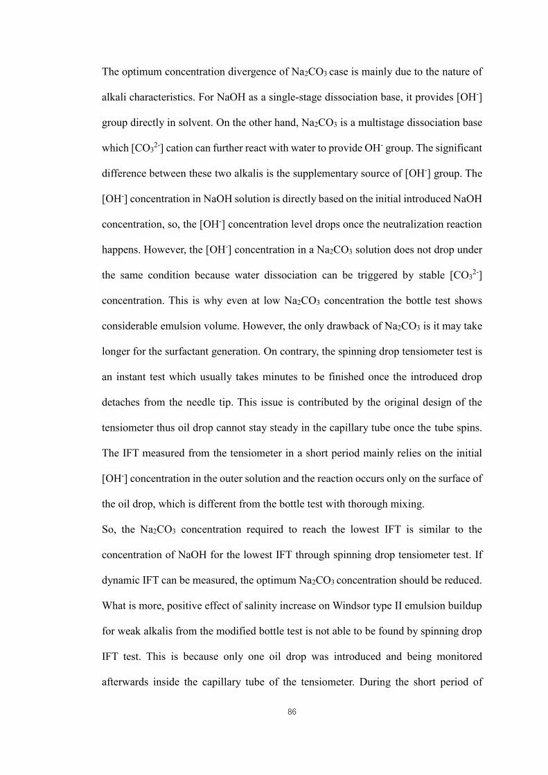
86
The optimum concentration divergence of Na2CO3 case is mainly due to the nature of
alkali characteristics. For NaOH as a single-stage dissociation base, it provides [OH-]
group directly in solvent. On the other hand, Na2CO3 is a multistage dissociation base
which [CO32-] cation can further react with water to provide OH- group. The significant
difference between these two alkalis is the supplementary source of [OH-] group. The
[OH-] concentration in NaOH solution is directly based on the initial introduced NaOH
concentration, so, the [OH-] concentration level drops once the neutralization reaction
happens. However, the [OH-] concentration in a Na2CO3 solution does not drop under
the same condition because water dissociation can be triggered by stable [CO32-]
concentration. This is why even at low Na2CO3 concentration the bottle test shows
considerable emulsion volume. However, the only drawback of Na2CO3 is it may take
longer for the surfactant generation. On contrary, the spinning drop tensiometer test is
an instant test which usually takes minutes to be finished once the introduced drop
detaches from the needle tip. This issue is contributed by the original design of the
tensiometer thus oil drop cannot stay steady in the capillary tube once the tube spins.
The IFT measured from the tensiometer in a short period mainly relies on the initial
[OH-] concentration in the outer solution and the reaction occurs only on the surface of
the oil drop, which is different from the bottle test with thorough mixing.
So, the Na2CO3 concentration required to reach the lowest IFT is similar to the
concentration of NaOH for the lowest IFT through spinning drop tensiometer test. If
dynamic IFT can be measured, the optimum Na2CO3 concentration should be reduced.
What is more, positive effect of salinity increase on Windsor type II emulsion buildup
for weak alkalis from the modified bottle test is not able to be found by spinning drop
IFT test. This is because only one oil drop was introduced and being monitored
afterwards inside the capillary tube of the tensiometer. During the short period of

87
operating time, the oil drop keeps its integrity and the surfactants generated by the
neutralization reaction only attach to the water/oil contact. Theoretically, additional salt
can force the in-situ surfactants move into the oil phase since the dissociated salt
occupies the space in aqueous phase. However, there is no significant oil or water
dispersion occurs for spinning drop IFT test case. Increasing the system salinity may
slightly compress the electrical double layer on the water/oil contact and exceeded
amount of salt deals nothing but breaking the emulsion stability and drive the IFT rise.
In general, the spinning drop IFT measurement is not sufficient to determine the
optimum condition for alkaline flooding thus its overall feasibility is inferior to the
modified bottle test.
As is mentioned by modified bottle test results, increasing alkaline concentration and
salinity alter the major emulsion type generated in the system. An optimum working
concentration and salinity of alkaline flooding can be found for highest total volume
of middle and top emulsions. Besides, since the emulsion type formed after
neutralization reaction determines which mechanism is capable of being achieved to
facilitate the oil recovery. Ideally, it will be a great convenience to predict the possible
emulsion generation during the alkaline flooding process through modified bottle test
to anticipate the alkaline flooding performance.
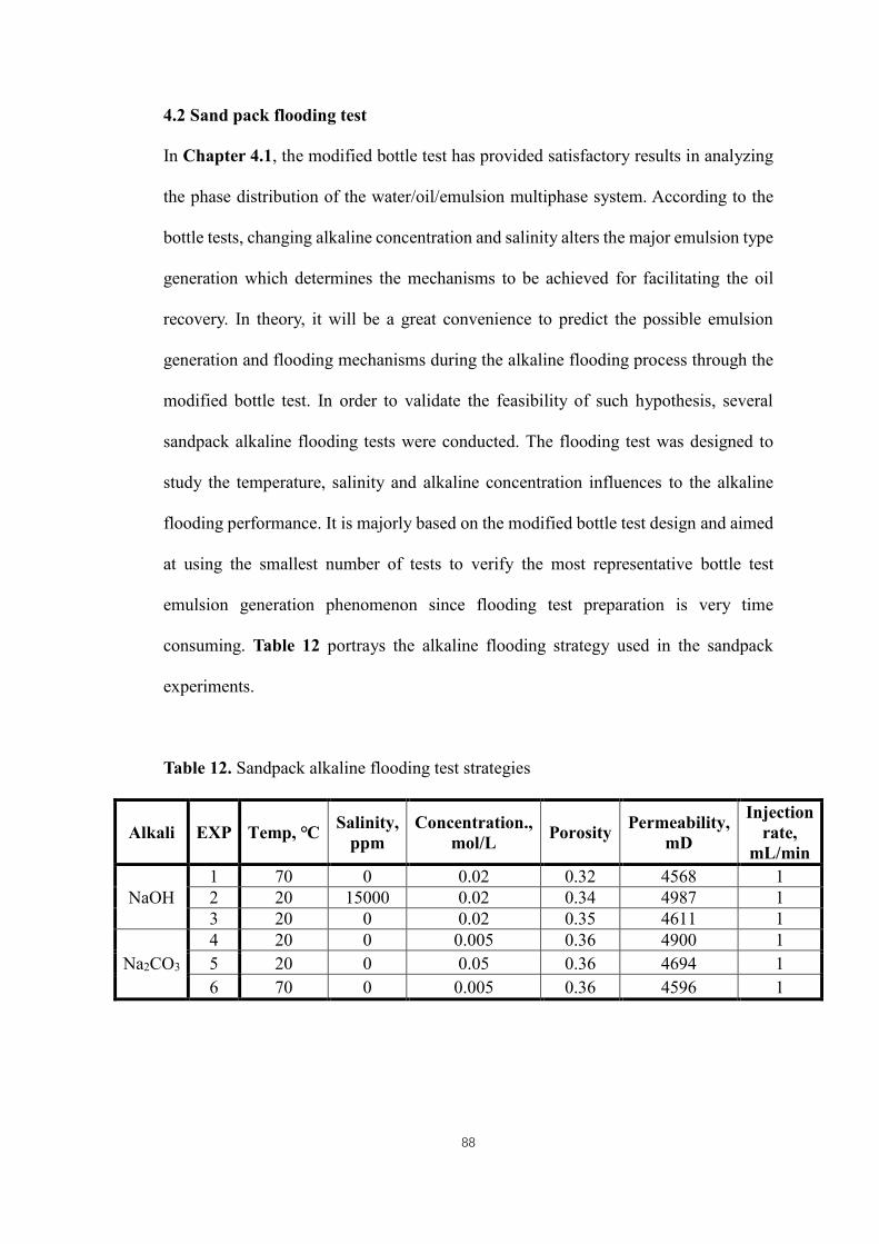
88
4.2 Sand pack flooding test
In Chapter 4.1, the modified bottle test has provided satisfactory results in analyzing
the phase distribution of the water/oil/emulsion multiphase system. According to the
bottle tests, changing alkaline concentration and salinity alters the major emulsion type
generation which determines the mechanisms to be achieved for facilitating the oil
recovery. In theory, it will be a great convenience to predict the possible emulsion
generation and flooding mechanisms during the alkaline flooding process through the
modified bottle test. In order to validate the feasibility of such hypothesis, several
sandpack alkaline flooding tests were conducted. The flooding test was designed to
study the temperature, salinity and alkaline concentration influences to the alkaline
flooding performance. It is majorly based on the modified bottle test design and aimed
at using the smallest number of tests to verify the most representative bottle test
emulsion generation phenomenon since flooding test preparation is very time
consuming. Table 12 portrays the alkaline flooding strategy used in the sandpack
experiments.
Table 12. Sandpack alkaline flooding test strategies
Alkali EXP Temp, ℃ Salinity,
ppm
Concentration.,
mol/L Porosity
Permeability,
mD
Injection
rate,
mL/min
NaOH
1 70 0 0.02 0.32 4568 1
2 20 15000 0.02 0.34 4987 1
3 20 0 0.02 0.35 4611 1
Na2CO3
4 20 0 0.005 0.36 4900 1
5 20 0 0.05 0.36 4694 1
6 70 0 0.005 0.36 4596 1
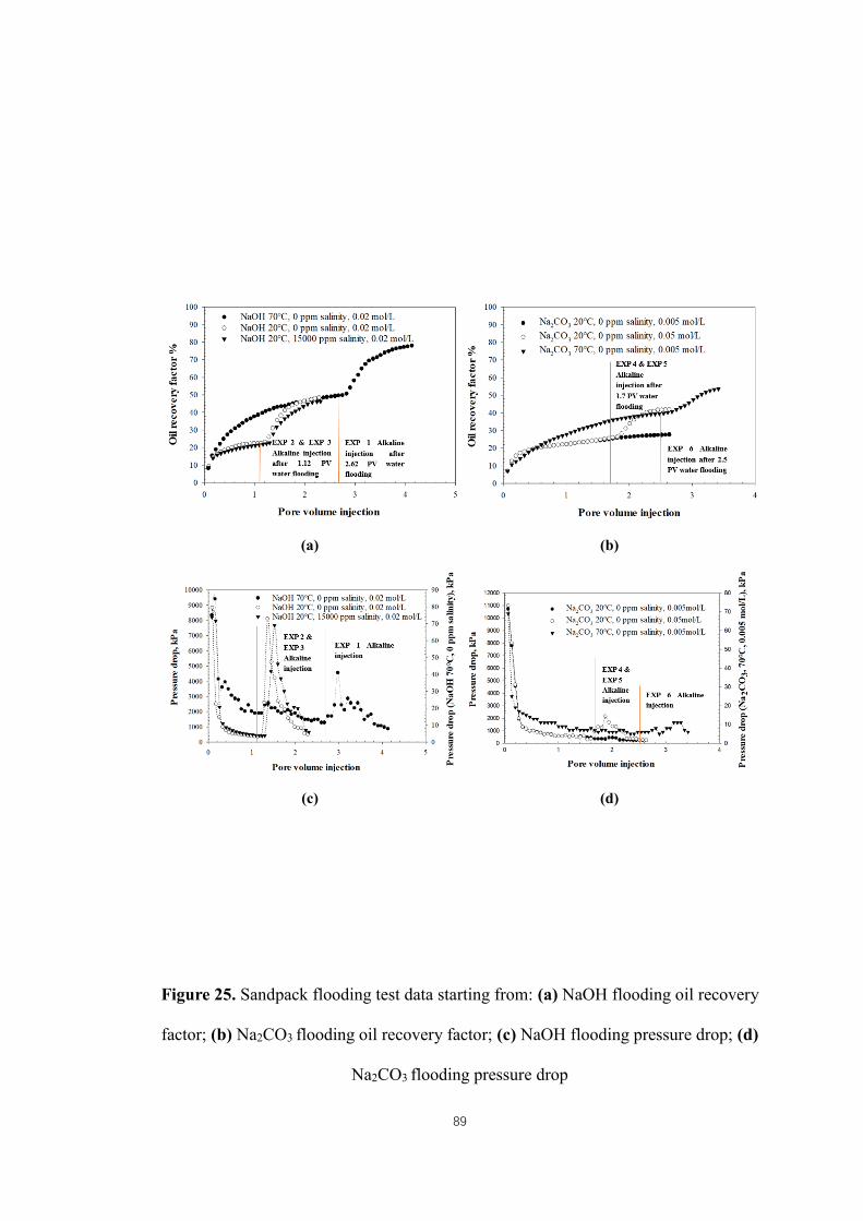
89
(a) (b)
(c) (d)
Figure 25. Sandpack flooding test data starting from: (a) NaOH flooding oil recovery
factor; (b) Na2CO3 flooding oil recovery factor; (c) NaOH flooding pressure drop; (d)
Na2CO3 flooding pressure drop
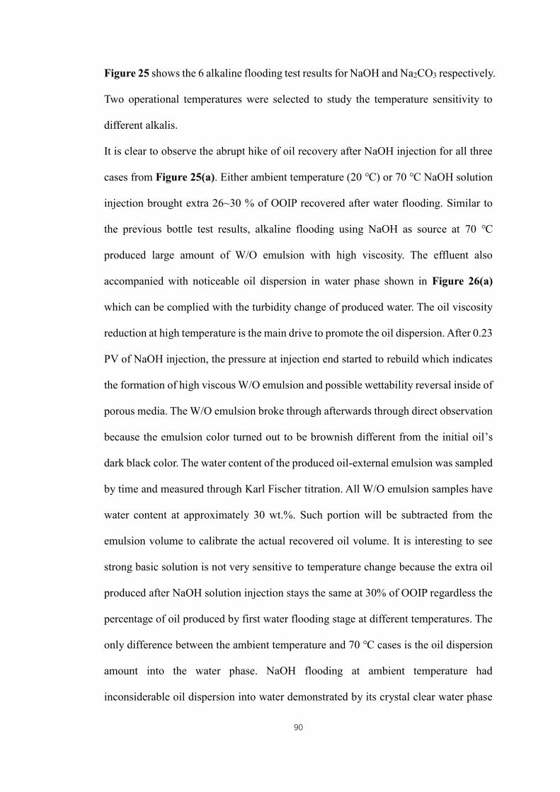
90
Figure 25 shows the 6 alkaline flooding test results for NaOH and Na2CO3 respectively.
Two operational temperatures were selected to study the temperature sensitivity to
different alkalis.
It is clear to observe the abrupt hike of oil recovery after NaOH injection for all three
cases from Figure 25(a). Either ambient temperature (20 ℃) or 70 ℃ NaOH solution
injection brought extra 26~30 % of OOIP recovered after water flooding. Similar to
the previous bottle test results, alkaline flooding using NaOH as source at 70 ℃
produced large amount of W/O emulsion with high viscosity. The effluent also
accompanied with noticeable oil dispersion in water phase shown in Figure 26(a)
which can be complied with the turbidity change of produced water. The oil viscosity
reduction at high temperature is the main drive to promote the oil dispersion. After 0.23
PV of NaOH injection, the pressure at injection end started to rebuild which indicates
the formation of high viscous W/O emulsion and possible wettability reversal inside of
porous media. The W/O emulsion broke through afterwards through direct observation
because the emulsion color turned out to be brownish different from the initial oil’s
dark black color. The water content of the produced oil-external emulsion was sampled
by time and measured through Karl Fischer titration. All W/O emulsion samples have
water content at approximately 30 wt.%. Such portion will be subtracted from the
emulsion volume to calibrate the actual recovered oil volume. It is interesting to see
strong basic solution is not very sensitive to temperature change because the extra oil
produced after NaOH solution injection stays the same at 30% of OOIP regardless the
percentage of oil produced by first water flooding stage at different temperatures. The
only difference between the ambient temperature and 70 ℃ cases is the oil dispersion
amount into the water phase. NaOH flooding at ambient temperature had
inconsiderable oil dispersion into water demonstrated by its crystal clear water phase
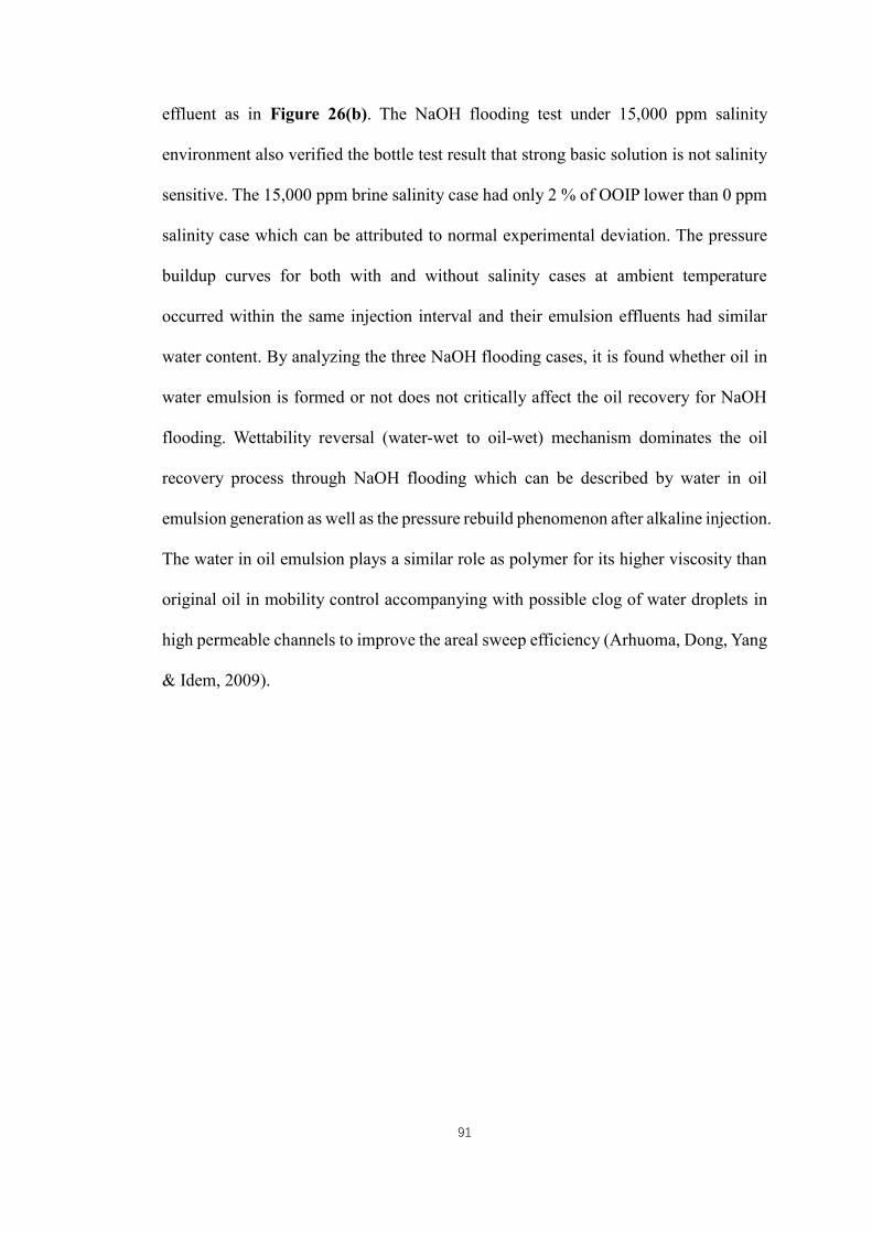
91
effluent as in Figure 26(b). The NaOH flooding test under 15,000 ppm salinity
environment also verified the bottle test result that strong basic solution is not salinity
sensitive. The 15,000 ppm brine salinity case had only 2 % of OOIP lower than 0 ppm
salinity case which can be attributed to normal experimental deviation. The pressure
buildup curves for both with and without salinity cases at ambient temperature
occurred within the same injection interval and their emulsion effluents had similar
water content. By analyzing the three NaOH flooding cases, it is found whether oil in
water emulsion is formed or not does not critically affect the oil recovery for NaOH
flooding. Wettability reversal (water-wet to oil-wet) mechanism dominates the oil
recovery process through NaOH flooding which can be described by water in oil
emulsion generation as well as the pressure rebuild phenomenon after alkaline injection.
The water in oil emulsion plays a similar role as polymer for its higher viscosity than
original oil in mobility control accompanying with possible clog of water droplets in
high permeable channels to improve the areal sweep efficiency (Arhuoma, Dong, Yang
& Idem, 2009).

92
Flooding
EXP
(a) NaOH
70 ℃
0.02 mol/L
(b) NaOH
20 ℃
0.02 mol/L
(c) Na2CO3
70 ℃
0.005 mol/L
(d) Na2CO3
20 ℃
0.05 mol/L
Effluents
after 0.35
PV of
alkaline
injection
Dominating
emulsion
type
O/W + W/O W/O O/W W/O
Figure 26. Emulsion type of effluent from sandpack
93
Identical to the bottle test prediction, as a weak alkaline solution, Na2CO3 flooding
tests showed different phenomenon from the NaOH flooding tests. Same PV of alkaline
injection at 70 ℃ produced extra 13 % of OOIP after water flooding which is half of
oil recovery through NaOH injection. However, there was no apparent pressure buildup
during the Na2CO3 injection stage due to different type of emulsion generation. The
effluent water phase with large amount of oil droplets suspension was observed during
alkaline injection which indicates the formation of O/W emulsion shown in Figure
26(c). The oil dispersion in water of such system is not very stable, so most oil droplets
accumulated after being settled for 48 hours. The produced oil during alkaline injection
was sampled and its water content is lower than 7 wt.%, thus the color of oil is still
black. There was a very slight pressure rebuild period during the final water flooding
stage which was also reported by Aminzadeh et al. (2016). It is believed to be caused
by small number of trapped oil droplets in pore throat so the pressure buildup was
insignificant. This phenomenon can be explained by the sufficient shear rate provided
under 1 mL/min injection rate thus most oil droplets are formed in suitable size that
can be produced with water (Bryan & Kantzas, 2007). The temperature sensitivity test
was also implemented to inject the same 0.005 mol/L (530 ppm) Na2CO3 solution after
water flooding at 20 ℃. The oil recovery factor of such case showed the 0.005 mol/L
Na2CO3 solution was not functioning at low temperature in contrast to the strong
alkaline solution cases. There are two possible assumptions that contribute to the
phenomenon. The first reason is due to the high oil viscosity at low temperature which
significantly reduces the oil emulsification possibility by alkaline solution under the
same shear rate. A second guess is rested on the temperature increase which provides
additional energy that facilitates the dissociation of weak alkali in aqueous phase. As
is known, the dissociation of weak alkali like Na2CO3 has multiple stages, generation

94
of OH- group is not instance but a reversible reaction with postponement as described
in following chemical equations (Acevedo et al., 2001).
Na2CO3H2O→ 2Na+ + CO3
2− [4.1]
CO32− + H2O
↔HCO3
− + OH− [4.2]
HCO3− +H2O
↔H2CO3 + OH
− [4.3]
High temperature condition may favor the positive reaction to generate sufficient [OH-]
group in the system and consequently reduces the IFT to a lower level. According to
the assumptions, 0.05 mol/L of Na2CO3 solution was injected after water flooding at
ambient temperature as well to study the weak alkaline concentration influence to oil
recovery. Although such concentration is somewhat out of the predefined optimum
concentration range, it is still workable since Na2CO3 is an excellent buffer solution
source. It remains the aqueous phase pH at 12 which is within the alkaline flooding
working pH range that keeps asphaltenes and resins active with alkalis (Bryan &
Kantzas, 2007; Ashrafizadeh et al., 2012; Rivas et al., 1997). As expected, the flooding
result fully matched with the previous bottle test result that W/O emulsion was
generated at high Na2CO3 concentration shown in Figure 25(d). In comparison to
Na2CO3 flooding running at optimum temperature and concentration, which
emulsification and entrainment mechanism accounted for the major driving force to
recover extra oil. High concentration of Na2CO3 injection case recovered extra 13 %
of OOIP relying on the W/O emulsion generation. In this case, no more oil dispersion
in water phase was observed from the effluent and the produced oil phase had more
than 20 wt.% of water content. The pressure from injection end also rose after Na2CO3
injection but was not as efficient as the NaOH flooding case. According to Wang et al.
(2010), Dong et al. (2012) as well as Bryan and Kantzas (2007), oil-external emulsion
viscosity increases with growing water content before converting to water-external
95
emulsion. Since water content of oil-external emulsion from high Na2CO3
concentration case is lower than NaOH cases, its lessened viscosity resulted in the
abbreviated pressure buildup peak and therefore recovered less oil than NaOH case.
Consequently, the Na2CO3 injection at high concentration is not very efficient because
its W/O emulsion quality is incomparable to that from NaOH injection; even though
both cases are dominated by wettability reversal (water-wet to oil-wet) and water
droplets entrapment mechanism, the injected Na2CO3 concentration is more than two
times of the NaOH concentration. The emulsion type alteration phenomenon in
sandpack flooding with increasing Na2CO3 concentration also matched well with
Na2CO3 concentration bottle test trend study. The low water content oil-external
emulsion in high Na2CO3 concentration case can be predicted from EXP8 in Table 11(a)
while oil dispersion cases occurred in other low Na2CO3 concentration bottle tests.
In spite of strong relationship between the flooding test results and bottle test
predictions, flooding test results can be solely summarized as well. Although some
outcomes have been pointed out by other researchers, following conclusions are still
solid evidence to prove the reproducibility of preceding studies on different oil types.
Firstly, Figure 27 plots a weak relationship between the dimensionless shear rate
change and corresponding oil recovery for both alkaline flooding cases. The
dimensionless shear rate of flooding tests can be calculated according to the injection
velocity, pressure change and rock properties based of following formulas (Bryan &
Kantzas, 2007).
γactual =4v
√kφ [4.4]
γapparent =4√
k
φΔP
Lμo [4.5]
γdim =γactual
γapparent [4.6]
96
The dimensionless shear rate is the ratio of actual shear rate to apparent shear rate.
During sandpack flooding test, constant flow injection was applied. Figure 27 shows
that periodic oil recovery drops with increasing dimensionless shear rate. It indicates
that more oil was recovered due to the shear rate increase during the alkaline injection.
It also implies that the emulsification process always accompanies with shear rate
increase in a system which from another angle proves that of great importance in a
bottle test to facilitate emulsification is enough shear force.

97
(a) 70 ℃ NaOH flooding oil recovery versus dimensionless shear rate
(b) 70 ℃ Na2CO3 flooding oil recovery versus dimensionless shear rate
Figure 27. Dimensionless shear rate and corresponding oil recovery every 10 min
during alkaline injection. According to the two figures, a weak linear relation can be
plot which less oil can be recovered at higher dimensionless shear rate. It means the
oil recovery performance of the alkali injection is better at higher shear rate.

98
Secondly, strong basic solution EOR like NaOH flooding theoretically has better
performance in oil recovery for large amount of high water content oil-external
emulsion generation. Type II emulsion has been proved of having the highest economic
efficiency by Aminzadeh et al. (2016). NaOH solution is also quiet versatile to different
reservoir environment under various temperature and salinity if putting multivalent
cation effect (Sun et al., 2017; Cooke et al., 1974) aside. The optimum NaOH solution
concentration is 0.02 mol/L or 800 ppm which is reasonable in use from point of
economic view. However, NaOH solution is corrosive to polymer stability if alkaline
polymer (AP) flooding is considered (Guo et al., 2017). Besides, the produced oil-
external emulsion is very hard to be separated which adds extra cost to later processing
(Ezzati, Gorouhi & Mohammadi, 2005; Barroso-Solares, Ointo, Nanni, Fragouli &
Athanassiou, 2018). What is more, it also causes environmental issues once injected
into the reservoir and deals harm to human health. Na2CO3 flooding on the other hand
is more environmental friendly for its mild dissociation process. Appropriate low
concentration of Na2CO3 solution injection under ideal temperature and salinity can
produce oil through emulsification and entrainment mechanism. The residual bulk oil
phase after water flooding is gradually emulsified into droplets and carried by aqueous
phase to be recovered. The essential difference between the two types of emulsion
produced after NaOH and Na2CO3 solution injection can be manifested by microscopic
observation in Figure 28. The Na2CO3 solution introducing water-external emulsion
type lifts partial of the cost from processing due to its low viscosity and instability
while it still provides a satisfying oil recovery.
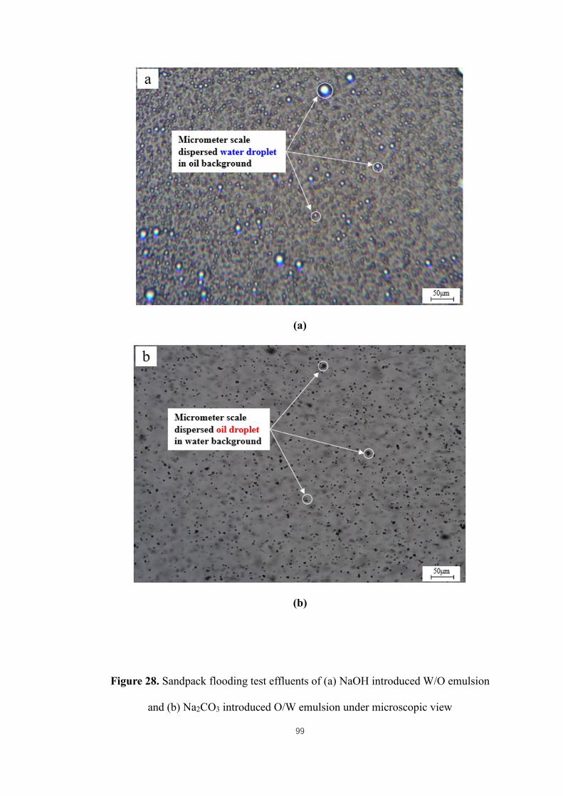
99
(a)
(b)
Figure 28. Sandpack flooding test effluents of (a) NaOH introduced W/O emulsion
and (b) Na2CO3 introduced O/W emulsion under microscopic view

100
The particle size distribution analysis based on microscopic images (Figure 29) shows
that the water droplets in oil-external emulsion have larger radius than oil droplet in
water-external emulsion. The water droplets in oil-external emulsion have higher
possibility to plug the high permeable zone thus improves the sweep efficiency and
contributes to the pressure buildup as well.
Figure 29. Emulsion particle size distribution analysis
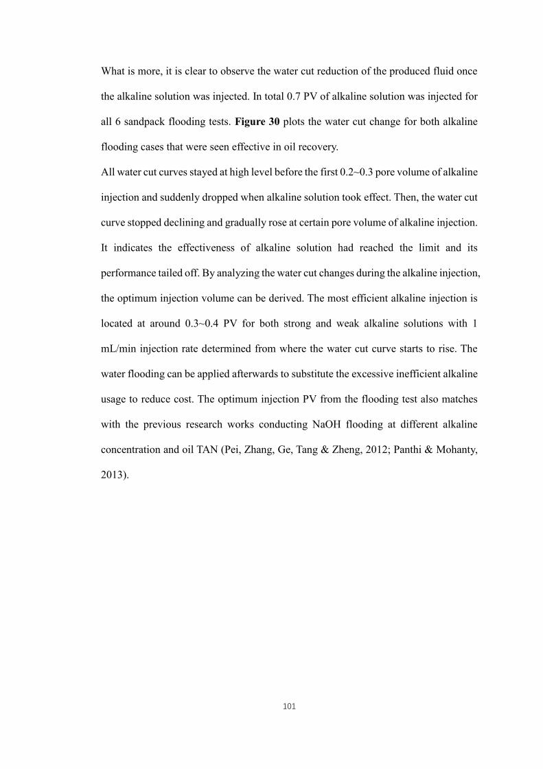
101
What is more, it is clear to observe the water cut reduction of the produced fluid once
the alkaline solution was injected. In total 0.7 PV of alkaline solution was injected for
all 6 sandpack flooding tests. Figure 30 plots the water cut change for both alkaline
flooding cases that were seen effective in oil recovery.
All water cut curves stayed at high level before the first 0.2~0.3 pore volume of alkaline
injection and suddenly dropped when alkaline solution took effect. Then, the water cut
curve stopped declining and gradually rose at certain pore volume of alkaline injection.
It indicates the effectiveness of alkaline solution had reached the limit and its
performance tailed off. By analyzing the water cut changes during the alkaline injection,
the optimum injection volume can be derived. The most efficient alkaline injection is
located at around 0.3~0.4 PV for both strong and weak alkaline solutions with 1
mL/min injection rate determined from where the water cut curve starts to rise. The
water flooding can be applied afterwards to substitute the excessive inefficient alkaline
usage to reduce cost. The optimum injection PV from the flooding test also matches
with the previous research works conducting NaOH flooding at different alkaline
concentration and oil TAN (Pei, Zhang, Ge, Tang & Zheng, 2012; Panthi & Mohanty,
2013).

102
(a)
(b)
Figure 30. Water cut data of (a) NaOH flooding and (b) Na2CO3 flooding

103
Finally, an important conclusion can be summarized from the sandpack flooding test
as well as the modified bottle tests. The emulsion type generated during the alkaline
flooding is not related to the exact alkali type but to the initial [OH-] group
concentration in aqueous phase the alkaline solution is able to provide. It is believed
that strong alkaline solutions can react with long-chain carboxylic acid while weak
alkaline solution at low concentration does not (Sun et al., 2017). Thus the surface
activity of in-situ surfactants under different cases varies. If the alkali dissociation rate
is fast enough to bring sufficient [OH-] group, the W/O emulsion tends to occur
regardless of the slight alkaline concentration adjustment. On the other hand, if the
alkali dissociation rate is slow, which usually happens to those alkalis with multistage
dissociation; W/O emulsion can also be formed given plentiful of alkaline
concentration. The high concentration of weak alkaline will compensate the slow
dissociation rate thus achieve the same emulsion type as strong alkalis. Nevertheless,
temperature change deals different influence from the alkaline concentration effect.
Through introducing internal energy into the fluid system, the weak alkaline solution
at low concentration which is originally not functional at ambient temperature is able
to recover extra oil after alkaline flooding. The temperature influence is essential to
weak alkaline flooding and oil in water emulsion occurred different from all other cases.
So, a new assumption regarding the alkaline flooding mechanism can be expressed:
The initial introduced [OH-] group concentration is the primary factor of an alkaline
flooding process according to its oil recovery performance. Temperature is also a
decisive factor but its importance is subordinate to the [OH-] group concentration.
When initial [OH-] group concentration is not enough, introducing additional energy
into the system facilitates the generation of in-situ surfactants. However, the actual in-
situ surfactant type varies under peculiar temperature. Due to the complexity of the oil

104
components with carboxylic acid group, it is tough to identify the exact substances
generated after neutralization reaction. Yet, in-situ surfactants with stronger
hydrophilic end tend to form at high temperature according to the effluents of flooding
tests from both strong and weak alkali cases. On contrary, in-situ surfactant with
stronger lypophilic end (long-chain molecule) is expected to be formed at ambient
temperature provided sufficient [OH-] group concentration in aqueous phase.

105
CHAPTER 5: Enhanced Numerical Simulation of Alkaline Flooding
CMG simulator has updated the geochemistry feature since version 2016 to enhance
the alkaline flooding model in regards of the ionic reactions including neutralization
reaction and retention. However, the implementation of geochemistry model requires
accurate aqueous phase ion concentrations monitoring of sandpack effluent end. It can
be achieved by conductivity measurement through ion selective electrodes; however,
the ever-changing pH value of the effluent is inevitable which deals great impact on
measurement precision between each trial. The experimental feasibility of the
geochemistry model is relatively low. What is more, emulsion is not represented by the
geochemistry model clearly. For high [OH-] concentration aqueous phase, water in oil
emulsion will be formed once the alkali is introduced into the sandpack. Due to the
high viscous nature of the oil-external emulsion and possible wettability alteration,
there will be noticeable pressure rebuild at alkali injection stage following water
flooding similar to polymer flooding process. The original water dominating channels
will be blocked by emulsion due to the wettability alteration and dispersed water
droplets in the emulsion also plugs the high permeable zone. The synergy of above
mechanisms results in the generation of oil bank at chemical flood front thus facilitates
the additional oil recovery. In general, emulsion generation is a very important
procedure which is controlled by in-situ surfactant concentration change for alkaline
flooding. An alkaline flooding model containing quantification of emulsion generation
is ideal for oil production prediction as more experimentally measurable constraints
are introduced thus weaken the uncertain relative permeability interpolation effect.
There are two major reactions considered in the enhanced alkaline flooding model. The
first is the neutralization reaction that generates in-situ surfactants. Another is the
emulsification process when oil external emulsion is formed. So, in spite of water, oil

106
and alkali in the CMG components, in-situ surfactant (AcNa) and emulsion will be
added to fulfill the construction of reaction 1 and 2 equations. The neutralization
reaction that generates carboxylate salts and water can be written in the form of:
NaOH + Oil → AcNa +Water
Conforming to the reaction 1 stoichiometry balance, the surfactant molecular weight is
assigned 22 g/gmol higher than oil to represent the substitution of [H+] ion by [Na+]
ion after neutralization reaction. Because the neutralization reaction mainly occurs on
carboxylic acid groups from the crude oil, and the [H+] ion exchange during the
reaction does not significantly affect the average total weight of the oil molecules, the
average surfactants molecular weight was assigned similar to the average crude oil
molecular weight.
The latter reaction 2 can be represented by following chemical equation: AcNa + Oil +
Water = Emulsion. According to the bottle test results, the average water content of oil-
external emulsion for optimum alkaline concentration is approximately 30 wt.%. Since
molecular weight of oil, in-situ surfactant and water are known, the average emulsion
molecular weight can be calculated. On the other hand, the amount of surfactant
required for generating 1 mol of emulsion can be derived by measuring the Na+
concentration change in the aqueous phase. This is because not all surfactants are
involved in the emulsification. By tracking the cation concentration difference between
initial stage and after emulsification, it is easy to know how many moles of surfactants
are brought to the oil phase by dispersed water. Therefore, the stoichiometry of reaction
2 is shown as following chemical equation:
1.41Water + 0.1986Oil + 0.00051AcNa → 2Emulsion
For in-situ surfactant generation equation of reaction 1, the stoichiometry of
neutralization reaction implies that every 1 mole of NaOH react with 1 mole of oil and

107
generate 1 mole of in-situ surfactants and 1 mole of water. Because the generation rate
of in-situ surfactant directly determines the emulsion quantity and the location of
emulsion formation in the sandpack, neutralization reaction rate has to be measured
through experimental means to make the simulation more representative. As NaOH
dissociates in aqueous phase acutely, neutralization reaction consumes the [OH-] group
straightly from alkali. Thus, the declination of pH value in the aqueous phase is
proportional to time as reaction undergoes. By monitoring the pH change, [OH-]
concentration reduction with time can be easily calculated thus the neutralization
reaction rate is able to be derived at certain temperature. Simultaneously, the Arrhenius
constant as well as the activation energy can be determined from the exponential
relationship of reaction rate and temperature. What is more, the viscosity of produced
emulsion from sand pack can be measured through cone and plate viscometer as a
component property input. The emulsion viscosity will have a positive effect on oil
recovery as emulsion mass fraction in oleic phase increases during the neutralization
reaction. The details of the experiment design and results have been introduced in
Chapter 2 and Chapter 3.
In general, four more reaction related parameters have been added to the alkaline
flooding model, which were depicted by keywords of FREQFAC, RENTH, EACT and
VISCA in the CMG data file. They stand for the reaction frequency factor (gmol/m3-
day, input unit dependent), reaction enthalpy (J/gmol), activation energy (J/gmol) and
viscosity without temperature control (cp) respectively. The first three parameters have
two sets of data for each of the two reactions (noted as 1 and 2). The RENTH2 is set to
0 since it is not theoretically a chemical process because there is no rearrangement of
the molecular or ionic structure. For better simulation prediction, temperature influence
on emulsion viscosity was not taken consideration regarding emulsion stability issue

108
at high temperature. Even though crude oil viscosity was measured at various
temperatures, it is only used for tuning the WinProp oil model. Alkaline flooding model
will be built based on room temperature condition only.
The alkaline flooding simulation in macroscopic view accompanying chemical
reaction and emulsion generation was rarely studied in the past. However, it is found
the chemical reaction is a very important segment which cannot be simply ignored
during alkaline flooding. Previous macroscopic chemical flooding usually considered
the relative permeability interpolation working with IFT change only to govern the
reservoir fluid flow; nevertheless, the prediction was hardly to be reliable without the
constraints from the chemical reaction part. Due to the complexity of the alkaline
flooding process, many parameters are involved in alteration of the flow condition
inside of reservoir. For the purpose of conducting further prediction and optimization
using the history matched model with confidence, the unknown parameters should be
reduced as many as possible before history matching the relative permeability
interpolation sets or other parameters.
5.1 Preliminary alkaline flooding model
5.1.1 Basic settings of preliminary alkaline flooding model
The CMG STARSTM model was built in order to match the alkaline flooding in
sandpack flooding test. The sandpack holder is in cylindrical shape and its length is 33
cm with 4 cm diameter. The sand packed in the holder is sealed by mesh-guarded
distributors at both ends to prevent sand leakage and the fluid can flow into the
sandpack evenly. In CMG reservoir modelling, the cylindrical reservoir was converted
to the cuboid block with same drainage area to simulate the 1-D reservoir. The cuboid
block was good enough to represent the cylindrical sandpack due to the usage of
distributors. The 33 cm long sandpack was splitted into 20 blocks to study the

109
saturation and pressure gradient along the flooding path.
The oil used in the flooding test is a dead oil sample and its properties are modelled by
CMG Winprop to match the lab data. The GC measured oil compositions were grouped
into 5 pseudo components with the final components as C45+. Afterwards, regression
parameters are conducted to alter the Pc, Tc, MW and viscosity related data of C45+ to
match its density and viscosity at 3 elevating temperatures from 20, 50 to 70 degrees
Celsius. The oil model after regression turns out to have a good agreement with the
experiment data. According to the regression report, the simulated density and
viscosity deviation is within 0.3% which is acceptable. Thus, the dead oil model fully
satisfies the simulation requirements. Simultaneously, the water, alkali, in-situ
surfactant as well as emulsion were added in the components section with proper
molecular weight, density and viscosity as mentioned. Gas phase was not considered
in simulation.
The rock-fluid properties were derived from the sandpack saturation tests. Arbitrary
data was assigned to the gas-liquid relative permeability curve since only water and oil
phases were involved inside of the sandpack. During the sandpack saturation process,
the rock properties, absolute permeability and connate water saturation can be
calculated. Once the sand was packed in the holder, the amount of sand used in packing
was measured. Initially, the sandpack was put straight and vacuumed by a vacuum
pump; then, brine was saturated from the bottom inlet by spontaneous suction.
Afterwards, the sandpack was laid horizontally and water was injected from the same
inlet end at different rates. The pressure drop at each rate was monitored when water
flow turned steady. So, the rock absolute permeability could be calculated based on
Darcy’s law, q = kA
μ
ΔP
L, which pressure drop is directly proportional to volumetric
flow rate. A linear relation could be plot in the figure and the permeability is derived

110
by the slope with known cross sectional area (A), water viscosity (μ) and the absolute
length of flow path (L). The whole sandpack was weighted again once permeability
test was finished to quantify the volume of water introduction. Usually, several pore
volumes of water have been injected into the sandpack and it is considered the
sandpack was fully saturated with water. Thus, the mass increase after permeability test
was contributed by water that occupies the porous media which indicates the whole
sandpack pore volume. Furthermore, the sandpack was put straight again and dead oil
was injected from the top inlet end to drainage the water out of the sand pack as oil
saturation process. The oil was injected above the water saturated sandpack at very
slow rate in order to prevent oil fingering during the drainage. The drainage process
usually took over 25 hours when bottom produced fluid is 100% oil. Then, the expelled
water volume was measured to calculate how much volume of water was left in the
sandpack and such volume fraction over initial saturated water volume is the connate
water saturation Swc. On the other hand, the irreducible oil saturation Soir can be
estimated after the second water imbibition in the sandpack after the drainage process.
According to the aforementioned tests, the rock properties as well as the saturation end
points for water-oil relative permeability curves can be input into the CMG BuilderTM
as initial rock-fluid model setup.
As mentioned, two sets of relative permeability curves will be used in CMG alkaline
flooding model to dynamically change the oil-water relative permeability with mass
transfer of alkalis by interpolation. The initial interpolation index, which is represented
by the logarithm capillary number (DTRAPW) is key value to control the interpolation
region. The capillary number is a dimensionless ratio of viscous force to capillary force
that is represented by: Nca = cμv
σ. C equals to 0.01 when μ is in centi poise, v in cm/s
and σ in dynes/cm. The capillary number during water flooding is calculated to be

111
6.95e-6. So the initial DTRAPW for relative permeability interpolation set 1 was -
5.158. When alkali is introduced, the minimum IFT measured is located at 2e-2
dynes/cm while the viscosity of alkaline solution is assumed to be the same as
deionized water. Consequently, the initial DTRAPW for relative permeability
interpolation set 2 was calculated to be -2.0791.
Finally, the adsorption was not considered for NaOH solution because it is operated at
low concentration and its dissociation as ionized form in aqueous phase has good
solubility to water. However, it is another story if the calcium ion in reservoir brine is
considered. In aqueous phase, calcium ion is easy to react with hydroxide group and
significantly consumes the alkali concentration since the calcium hydroxide generated
from the reaction is slightly soluble to water. So, in addition to the two reactions during
the emulsification process, another reaction regarding Ca(OH)2 generation and
precipitation is taken into consideration to describe the multivalent effects on alkaline
flooding.
Based on above simulation processes and theories, a preliminary CMG alkaline
flooding model was built with some random initial inputs at reasonable ranges. The
multivalent cation effects will be discussed in Chapter 5.2.2 once the representative
alkaline flooding is built. The sensitivity of each parameter in the model except relative
permeability curves are tested by CMG CMOST which are shown in the next section.

112
5.1.2 Sensitivity analysis of alkaline flooding model
Based on the simulation model, there are more than 14 parameters require value input.
10 out of 14 parameters can be derived from the experiment tests. Since these
parameters can be directly determined by experiments, they are not able to be further
tuned even if their values change deal great influence to the flooding performance.
Whether the rest parameters have significant influence to the oil production will be
evaluated by the CMOST sensitivity analysis. The sensitivity analysis process simply
edits the targeted parameter in the data file at values in 110 discrete sampling settings.
These parameters include but not limited to sandpack permeability, emulsion viscosity,
reaction frequency factor (FREQFAC1) and activation energy (EACT) of reaction 1.
Thus, the rest tunable parameters are grouped into four portions based on their
characteristics which contains 4 parameters related to logarithm capillary numbers of
relative permeability curves for interpolation, 4 parameters that fit the power position
in Corey correlation to alter the curvature of the relative permeability curves, reaction
frequency factor of reaction 2 (FREQFAC) as well as reaction enthalpy of
saponification (RENTH). The sensitivity analysis was conducted according to the later
three groups since relative permeability obviously has the highest effect on oil recovery
for changing the core properties of fluid flow in the formation. The parameter sequence
of history matching was determined based on their sensitivity rating from strong to
weak trend. The following study uses cumulative oil recovery at standard condition as
the reference to show the parameter sensitivity. The first parameter tested was reaction
enthalpy of reaction 1. Its originally defined to be 0 J/gmol which means this parameter
is ignored. The upper limit of 100 J/gmol was assigned and 100 experiment were
conducted to observe the oil recovery change. According to Figure 31, the effecting
area of enthalpy change is minor and it only takes effect near the end of alkaline
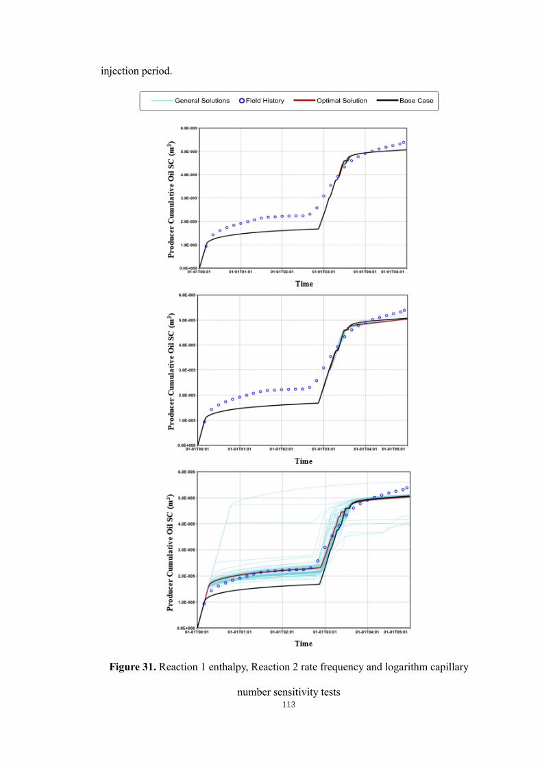
113
injection period.
Figure 31. Reaction 1 enthalpy, Reaction 2 rate frequency and logarithm capillary
number sensitivity tests
114
The reaction 2 frequency factor of emulsification process was studied afterwards. Its
originally value of 0.435 was randomly assigned and the data range of 0.1 to 10 was
set for the sensitivity analysis. From the figure, it is found that the change of reaction
2 frequency factor affects the whole alkaline injection process and later water flooding
which has a wider influence than enthalpy in reaction 1. This is reasonable because the
rate of emulsification process determines the amount of high viscous emulsion
generation.
Finally, the logarithm capillary numbers of relative permeability curves in 2
interpolations are adjusted to test their sensitivity. Since the relative permeability curve
in interpolation set 1 is designed for water flooding while alkaline flooding represented
relative permeability curve is in interpolation set 2, the capillary number in
interpolation set 1 should be smaller than the capillary number in interpolation set 2.
Therefore, their logarithm form should follow the same order. A hard constraint was
assigned when DTRAPW1 and DTRAPW2 are adjusted together, which DTRAPW1
< DTRAPW2 disregarding their predefined data ranges. For simplicity, the DREAPN
values are set equal to DTRAPW values. According to the test result figure, the
capillary number change has great influence to the whole flooding process thus its
sensitivity is the highest.
Once the sensitivity analysis has been completed, the sensitivity rating was produced
from high to low, which starts with the logarithm capillary number (DTRAP), reaction
2 frequency factor followed by reaction 1 enthalpy. The history data match of the
preliminary alkaline flooding model is aiming at ultimately simulate the experiment
result as close as possible. Once the parameters are tuned through CMOST, their values
will not be changed in any case for further study to keep the simulation consistency.
As is mentioned, the preliminary model of alkaline flooding is built based on

115
experience. This model was put into the CMOST to conduct history match. Primarily,
the relative permeability curves were tuned to match injector well bottom-hole pressure,
cumulative oil production and cumulative water production at standard condition.
Initially, it has 15.87% global history match error comparing to the experiment results.
The Corey correlation was used to alternate the curvature of relative permeability curve
based on end saturation points provided by the simulator. Following power-law
equations were used to calculate the water and oil relative permeability curves
respectively while gas saturation is not considered. According to the effluent analysis
from flooding test, the maximum oil and water relative permeability were assigned to
be 1.
kro = kro,max × (1−Sw−Sor
1−Sor−Swc)no [5.1]
krw = krw,max × (Sw−Swc
1−Sor−Swc)nw [5.2]
4 parameters including 2 pairs of no and nw were tuned within the data range from 0.01
to 10. Since relative permeability curves in interpolation set 2 stands for alkaline
flooding region; theoretically, the oil curve should become flatter and water curve
needs to be more arch to facilitate the oil flow in the sandpack. Because CMG
simulation focuses more on a macroscopic view regarding fluid flow, relative
permeability curves majorly play the role as fluid “mobility indicator” to illustrate fluid
flow capability, rock wettability is a separate input in rock-fluids section which cannot
be directly interpreted by initial relative permeability curve sets of the CMG simulator.
Thus, wettability alteration is not represented by the shift of two relative permeability
interpolation sets. When it comes to history data match by tuning power-law
parameters, no1 and nw1 are defined to be smaller than no2 and nw2 in any case no matter
the selections of their data range to satisfy the curve shift theory.
The global history match error of bottom-hole pressure, cumulative oil and water

116
production was reduced by 5.86%. Figure 32 shows the final history matched relative
permeability curves in interpolation set 1 and 2.
Then, the second sensitive parameter group of logarithm capillary number was history
matched which further reduce the global history match error from 5.68% to 4.56%. It
can be seen that the cumulative oil recovery figure well matches the water flooding
period and the turning point during alkaline injection is getting closer to the experiment
data.
Afterwards, the reaction 2 frequency factor tuning slightly increased the final oil
recovery to better match the simulation curve with the experiment data. Finally, the
reaction 1 enthalpy was tuned to have minor adjustment of the second turning point
near the end of alkaline flooding. After four stages of history match for pure alkaline
injection model, the final model global history match error was reduced to 4.47%. The
history match results of above four stages are shown in Figure 32. It can be found that
the simulated oil recovery gradually gets closer to the experiment data by tuning the
related parameters in sequence.
Figure 33 shows the injection bottom-hole pressure, cumulative oil and water
production at standard condition along with the experiment data respectively. It is clear
to see that current model is representative as it matches with the experiment data well
under the same condition.
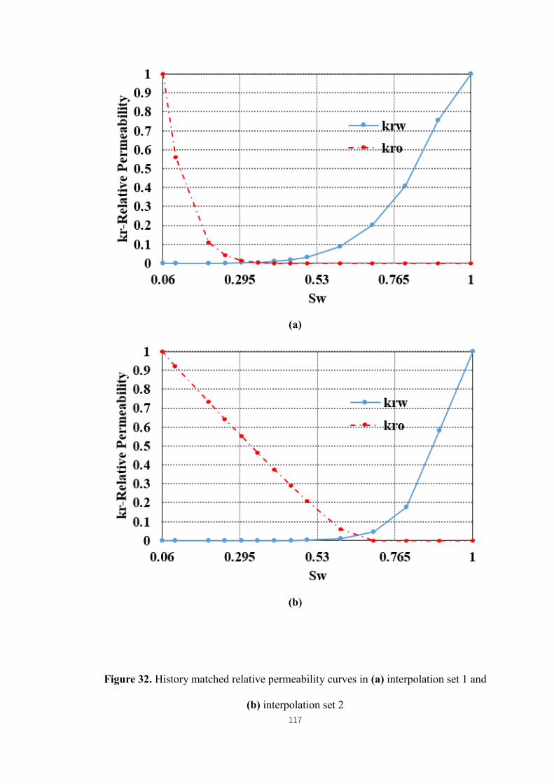
117
(a)
(b)
Figure 32. History matched relative permeability curves in (a) interpolation set 1 and
(b) interpolation set 2
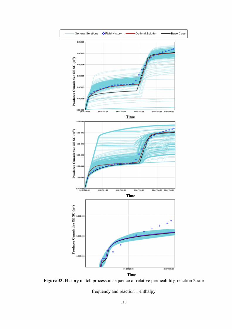
118
Figure 33. History match process in sequence of relative permeability, reaction 2 rate
frequency and reaction 1 enthalpy
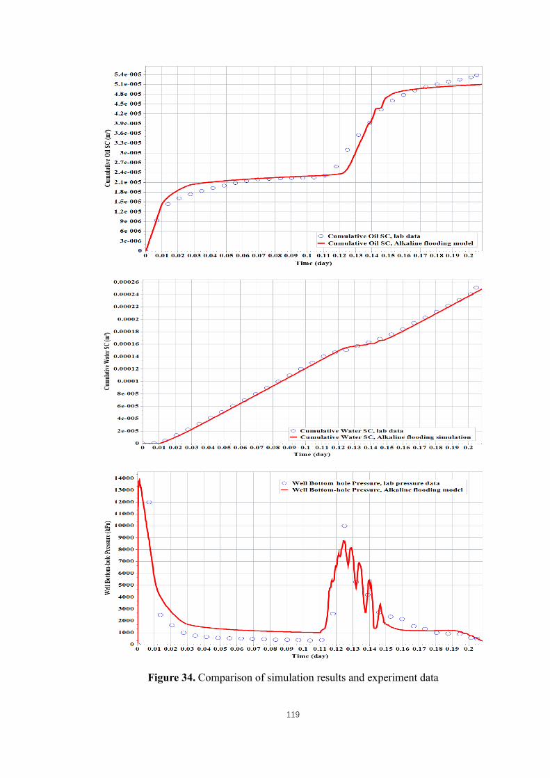
119
Figure 34. Comparison of simulation results and experiment data

120
The cumulative oil recovery, cumulative water recovery and pressure drop of the final
history matched NaOH flooding model are plot with the experiment data in Figure 34.
It is clearly to see that the simulation results have good agreement with history data.
Analyzing the oil saturation distribution of the simulation model can observe an oil
bank was generated during the alkaline flooding depicted in Figure 35. The residual
oil saturation after the initial water flooding is 0.75 which means only 20 % of OOIP
can be produced by water flooding. The oil bank is formed right after the alkali
injection starting at the 4th block. Its volume gradually increases with propagation and
the maximum oil bank oil saturation reaches 0.89. The blocks swept by the oil bank
leaves 0.55 to 0.60 oil saturation indicating additional 20 % of OOIP is recovered by
the alkaline flooding process.
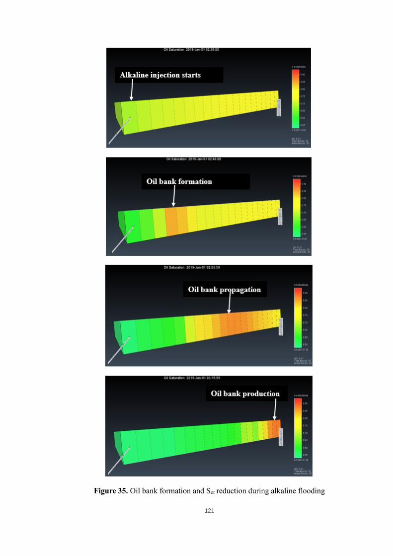
121
Figure 35. Oil bank formation and Sor reduction during alkaline flooding

122
5.2 History matched alkaline flooding simulation
5.2.1 Alkaline flooding prediction and optimization
Several alkaline injection predictions can be conducted based on the history matched
alkaline flooding model. Of significance to the sandpack undergoing alkaline flooding
in ideal condition are alkaline injection quantity/time as well as the flooded alkaline
concentration. Thus, various NaOH concentrations injection were tested at first by
alkaline flooding model to determine the optimum injection concentration primarily.
The cumulative oil recovery varies significantly depends on the type of injected fluid
after 0.11 days according to Figure 36(a). It can be seen that further water flooding
can barely increase the oil production due to the poor mobility of oil at high water
saturation. On the other hand, 0.0001 mol% NaOH injection effectively boosts the oil
recovery after water flooding. The oil recovery gradually increases at higher NaOH
concentration but concentration ceiling occurs when it hits 0.00034 mol% and further
high concentration NaOH injection does not bring extra oil production.
Correspondingly, the oil production curve of NaOH injection at concentration of
0.00034 mol%, 0.00035 mol%, 0.0004 mol% and 0.00045 mol% overlap with each
other which means the NaOH performance limit has been reached. Based on the
production prediction, the optimum NaOH concentration is determined to be 0.00034
mol% equals to 0.019 mol/L and such value is close to the NaOH concentration having
the minimum IFT with oil measured by spinning drop tensiometer that performed
outstandingly during emulsification process in bottle test.

123
(a)
(b)
(c)
Figure 36. Simulation results by escalating concentration NaOH flooding
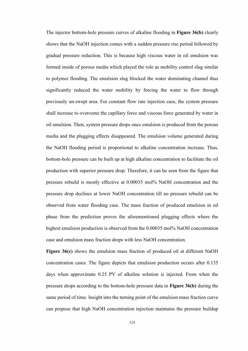
124
The injector bottom-hole pressure curves of alkaline flooding in Figure 36(b) clearly
shows that the NaOH injection comes with a sudden pressure rise period followed by
gradual pressure reduction. This is because high viscous water in oil emulsion was
formed inside of porous media which played the role as mobility control slug similar
to polymer flooding. The emulsion slug blocked the water dominating channel thus
significantly reduced the water mobility by forcing the water to flow through
previously un-swept area. For constant flow rate injection case, the system pressure
shall increase to overcome the capillary force and viscous force generated by water in
oil emulsion. Then, system pressure drops once emulsion is produced from the porous
media and the plugging effects disappeared. The emulsion volume generated during
the NaOH flooding period is proportional to alkaline concentration increase. Thus,
bottom-hole pressure can be built up at high alkaline concentration to facilitate the oil
production with superior pressure drop. Therefore, it can be seen from the figure that
pressure rebuild is mostly effective at 0.00035 mol% NaOH concentration and the
pressure drop declines at lower NaOH concentration till no pressure rebuild can be
observed from water flooding case. The mass fraction of produced emulsion in oil
phase from the prediction proves the aforementioned plugging effects where the
highest emulsion production is observed from the 0.00035 mol% NaOH concentration
case and emulsion mass fraction drops with less NaOH concentration.
Figure 36(c) shows the emulsion mass fraction of produced oil at different NaOH
concentration cases. The figure depicts that emulsion production occurs after 0.135
days when approximate 0.25 PV of alkaline solution is injected. From when the
pressure drops according to the bottom-hole pressure data in Figure 36(b) during the
same period of time. Insight into the turning point of the emulsion mass fraction curve
can propose that high NaOH concentration injection maintains the pressure buildup
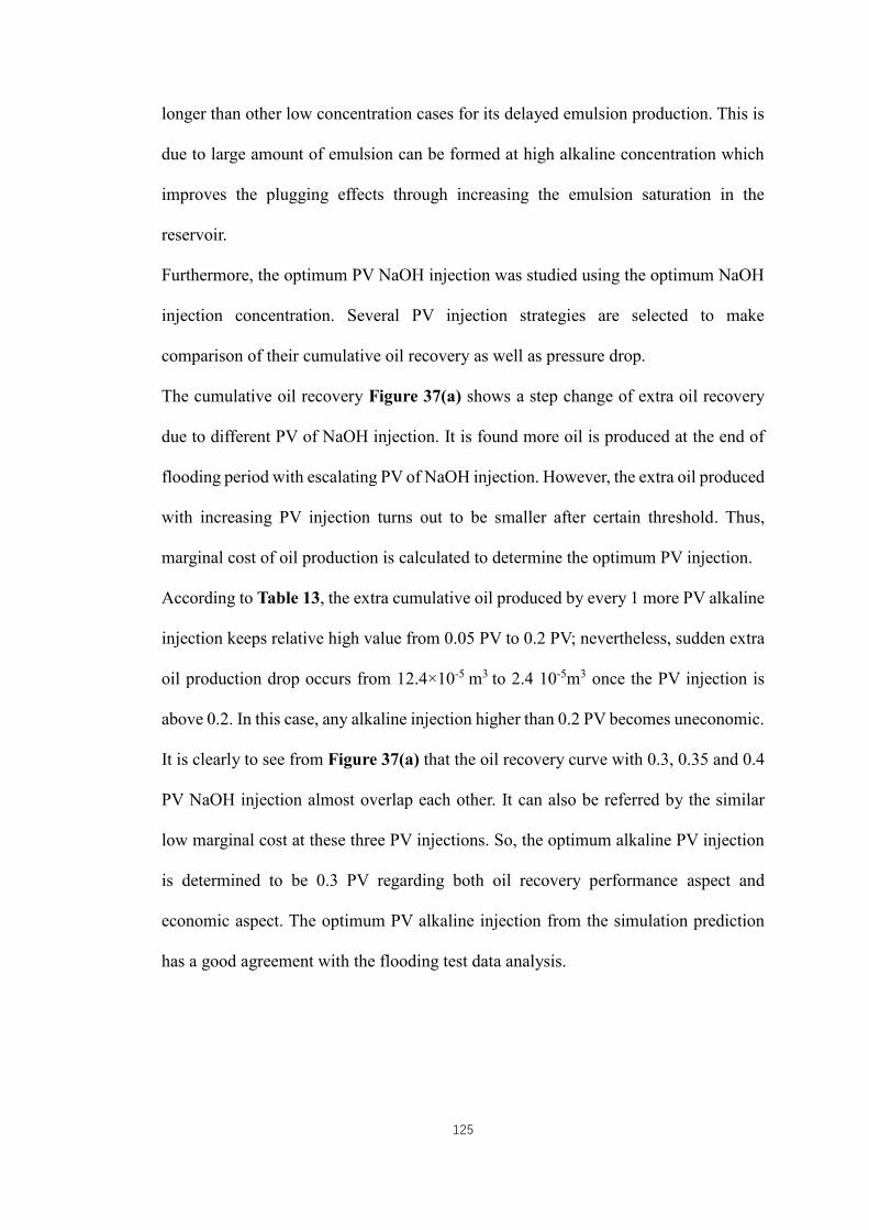
125
longer than other low concentration cases for its delayed emulsion production. This is
due to large amount of emulsion can be formed at high alkaline concentration which
improves the plugging effects through increasing the emulsion saturation in the
reservoir.
Furthermore, the optimum PV NaOH injection was studied using the optimum NaOH
injection concentration. Several PV injection strategies are selected to make
comparison of their cumulative oil recovery as well as pressure drop.
The cumulative oil recovery Figure 37(a) shows a step change of extra oil recovery
due to different PV of NaOH injection. It is found more oil is produced at the end of
flooding period with escalating PV of NaOH injection. However, the extra oil produced
with increasing PV injection turns out to be smaller after certain threshold. Thus,
marginal cost of oil production is calculated to determine the optimum PV injection.
According to Table 13, the extra cumulative oil produced by every 1 more PV alkaline
injection keeps relative high value from 0.05 PV to 0.2 PV; nevertheless, sudden extra
oil production drop occurs from 12.4×10⁻⁵ m3 to 2.4 10-5m3 once the PV injection is
above 0.2. In this case, any alkaline injection higher than 0.2 PV becomes uneconomic.
It is clearly to see from Figure 37(a) that the oil recovery curve with 0.3, 0.35 and 0.4
PV NaOH injection almost overlap each other. It can also be referred by the similar
low marginal cost at these three PV injections. So, the optimum alkaline PV injection
is determined to be 0.3 PV regarding both oil recovery performance aspect and
economic aspect. The optimum PV alkaline injection from the simulation prediction
has a good agreement with the flooding test data analysis.

126
(a)
(b)
(c)
Figure 37.Simulation results by different PV of NaOH injection
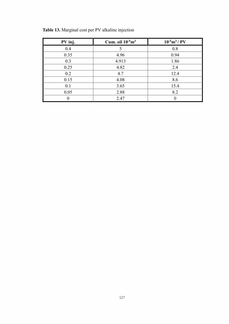
127
Table 13. Marginal cost per PV alkaline injection
PV inj. Cum. oil 10-5m3 10-5m3 / PV
0.4 5 0.8
0.35 4.96 0.94
0.3 4.913 1.86
0.25 4.82 2.4
0.2 4.7 12.4
0.15 4.08 8.6
0.1 3.65 15.4
0.05 2.88 8.2
0 2.47 0

128
Besides, it can be seen from the pressure drop Figure 37(b) that insufficient alkaline
injection deals early pressure reduction for deficient emulsion generation being not
able to compensate the fast depletion of emulsion which has been recovered with oil.
This phenomenon can also be verified by above emulsion mass fraction in recovered
oil Figure 37(c) where the emulsion production of 0.05 PV and 0.15 PV alkaline
injection is not comparable to the cases of 0.25 PV and 0.35 PV alkaline injection when
emulsion generation is sufficient and reservoir pressure is well maintained. Due to the
limit of CMG simulation which majorly focuses on the macroscopic fluid flow
calculation, the pressure rebuild is the calculation based on the interpolated relative
permeability determined by each block’s current alkaline concentration. As injected
NaOH concentration is fixed, all curves share the same pressure rise trend during
alkaline flooding and only the pressure drop section depicts their difference. This is the
nature of CMG simulator which cannot be further modified without deep manipulation.
5.2.2 Alkaline flooding model considering multivalent cation effects
In this section, the reservoir brine’s multivalent cation effects were modelled and
studied. For simplicity, brine NaCl salinity is omitted since extra monovalent cation
deals minor influence to the oil-external emulsification process. Ca2+ was used as the
source of multivalent cation in the form of CaCl2 which reacts with NaOH and generate
solid precipitation. A new reaction was included in the simulation model to present
such precipitation reaction that consumes the injected alkali as following.
2NaOH + CaCl2 → 2NaCl + Ca(OH)2
In which Ca(OH)2 was defined as the solid phase. As correct molecular weight of the
new components were assigned, no stoichiometry error was shown since it fully
satisfies the material balance. The reaction frequency factor of reaction 3 was measured
based on the same pH monitoring method which has been discussed in Chapter 3.1.4.

129
The final calculated average reaction 3 rate is about 106 L/mol-day. As mentioned, the
precipitation reaction at such high rate can barely use the pH method to acquire reliable
pH change with time. So, an additional sandpack flooding test was conducted at this
stage and it is designed to be the copy of the previous room temperature NaOH flooding
test except the brine substitutes the deionized water in saturation and flooding period.
The brine was prepared as a 0.005 mol/L CaCl2 solution to study the negative effects
of multivalent cation to NaOH flooding performance. Unfortunately, the original sand
sample for sandpack flooding test was lost. So, a type of new Ottawa sand was selected
which has similar size distribution to the previous sand from the microscope
observation. The NaOH flooding in deionized water saturated sandpack with new sand
case (EXP5) was conducted to make comparison to the flooding test EXP3.
Table 14. Two NaOH flooding sandpack properties comparison
Experiments Sand packed/ g Porosity Permeability/
mD
Soi
EXP3 761.12 0.34 4987.00 0.94
EXP5 757.71 0.36 8373.00 0.933
130
Figure 38. Comparison of NaOH flooding results of EXP3 and EXP5

131
The Table 14 shows the comparison of the sandpacks’ properties and the flooding
results are provided as well. The EXP5 extends the water flooding period while remain
the NaOH PV injection the same in order to make the comparison of two alkaline
flooding periods straightforwardly in Figure 38. It can be seen that the alkaline
flooding performance after water flooding in both sandpack experiments are similar in
spite of pressure change at injection end. This is mainly due to the sandpack
permeability of EXP5 is higher than that of EXP3 thus contributes to lower maximum
pressure drop in EXP5. Nevertheless, the cumulative oil recovery is still representative
using the new sand sample. Then, same sandpack flooding test were conducted using
CaCl2 solution substituting deionized water following NaOH injection (EXP6). The
test results were provided in Figure 39 in comparison with EXP5. From the figure, the
cumulative oil recovery clearly shows the significant oil recovery reduction in alkaline
flooding period after substituting deionized water with brine as the reservoir fluid. The
additional oil recovery after NaOH flooding was almost halved comparing to EXP5
and the pressure rebuild cannot reach as high as the initial maximum pressure during
water flooding. Besides, the pressure rebuild point experienced a short delay because
most of the NaOH at flood front was depleted for reacting with the CaCl2 in porous
media. Correspondingly, the water cut of effluent after alkaline flooding was higher in
EXP6 which contributed to less oil recovery. The multivalent cation’s negative effects
on alkaline flooding performance was proved based on the sandpack flooding test.

132
Figure 39. Comparison of NaOH flooding results of EXP5 and EXP6

133
What is more, the EXP6 flooding test was used to calibrate the precipitation reaction
rate for the simulation study. The calibration process is designed to match the simulated
effluent CaCl2 mole fraction in water phase with experimentally measured Ca2+ ion
concentration of the aqueous effluents which are collected from the sandpack flooding
test through tuning the reaction 3 frequency factor. The Mettler Toledo perfectION
comp CA electrode is used in this case to measure accurate Ca2+ concentration in
aqueous phase. Because the effluent was collected every 10 mL per test tube, the time
interval of each ion concentration measurement varies from 10 min to 30 min in case
the aqueous phase is inadequate in one test tube to fulfill the minimum volume required
by the test. Each aqueous sample was filtrated by the Buchner funnel to remove the
organic content for better electrode test accuracy. Figure 40(a) shows the schematic
diagram of ion concentration measurement setup.
The sample selection was majorly accumulated near the NaOH injection stage where
the Ca2+ concentration may significantly change. Table 15 shows the
Ca2+ concentration of effluent from EXP6 at different time intervals followed by the
converted CaCl2 mole fraction in water phase.

134
Table 15. EXP6 effluent Ca2+ concentration change with time
Time
interval
Ca2+,
mol/L
CaCl2 mol fraction
W producer
100-150 min 0.00504 0.00009072
200-250 min 0.00504 0.00009072
260 min 0.00504 0.00009072
270 min 0.00503 0.00009054
280 min 0.00353 0.00006354
290 min 0.000303 0.000005454
300-310 min 0.0000754 1.3572E-06
320-330 0.0000677 1.2186E-06
340-350 0.0000444 7.992E-07
360-370 0.00000493 8.874E-08
380-390 0.0000134 2.412E-07
400 min 0.00137 0.00002466
410 min 0.00246 0.00004428
420 min 0.00318 0.00005724
430 min 0.00369 0.00006642
440 min 0.00394 0.00007092
450 min 0.00411 0.00007398
The Mettler Toledo s220 ion meter has the measurement range from 1e-9 mol/L to
9.99e9 mol/L according to its manual. So the measurement accuracy was pretty high.
The Table 15 data has been fit into their corresponding time line along the flooding
test EXP6 and the dot plot in Figure 40(b) shows how Ca2+ concentration was cut due
to the NaOH injection and later rebuild during subsequent water flooding process. Time
points before the alkaline flooding stage were added based on 100-150 min data to
make the whole figure complete.
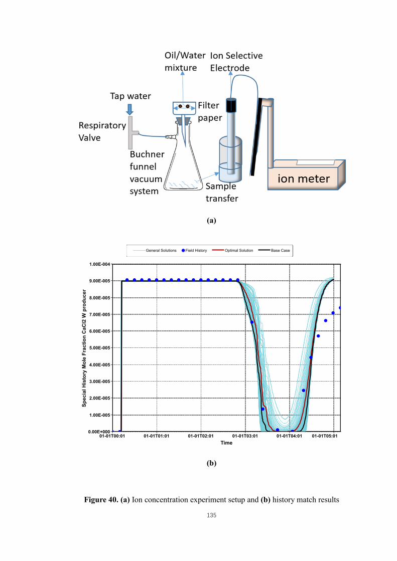
135
(a)
(b)
Figure 40. (a) Ion concentration experiment setup and (b) history match results

136
The history match of CaCl2 case was conducted by CMG CMOST to tune the reaction
3 rate frequency factor in the data range from 1 to 1000 staring from 400. The final
matched results are provided in Figure 40(b). The history matched model has the
optimum FREQFAC3 value to be 130 L/mol-s which is very close to the pH reaction
rate test results at approximate 110 L/mol-s. Thus, the simulation result proves the
feasibility of reaction rate measurement based on pH change from another angle.
Therefore, the simulation model considering multivalent cation effects was completed.
Then, several prediction and optimization studies can be conducted according to the
existence of Ca2+ in the reservoir. Based on the status report, the total dissolved solid
(TDS) of the heavy oil formation brine is about 160000 ppm in which CaCl2 occupies
40000 ppm. So, 0.0065 mol% of CaCl2 solution is assigned to the alkaline flooding
model with 0.3 PV of NaOH injection. Figure 41(a) clearly shows the negative effects
on oil recovery due to the existence Ca2+ ion. The additional oil recovered by alkaline
flooding is only one thirds of the deionized water case. That is why many alkaline
flooding pilot tests were reported ineffective considering the adjacent aquifer that
continuously provides brine to the reservoir. To solve this problem, we can either
increase the injected NaOH solution concentration or conduct preflush to reduce the
reservoir salinity. Increasing the NaOH PV injection also benefits the oil recovery but
it is not recommended to be simulated by current model and it will be discussed in the
Chapter 5.2.3.

137
(a)
(b)
(c)
Figure 41. CaCl2 effects on oil recovery by NaOH flooding

138
The first trial of increasing the NaOH injection amount is by adding extra 0.0001 mol%
of NaOH per simulation to see effects. Through simulation results shown by Figure
41(b), it can be concluded that increasing injected NaOH concentration can effectively
boost the oil recovery by compensating the depleted NaOH with additional alkali
quantity. However, the high salinity nature of the reservoir brine makes this method
uneconomic for tripling the alkali concentration only brings 65% more of oil recovery.
What is more, the preflush method is also simulated to see effects. There are several
preflush types in fields including fresh water, softened reservoir brine and brackish
water (Mayer, et al., 1983). The latter two has salinity higher than fresh water but
significantly lower than reservoir brine considering the cost of fresh water and the
reservoir location. So, the preflush with different CaCl2 concentrations at 0.9 PV were
simulated and the oil recovery and CaCl2 mole fraction produced in water phase were
compared.
The oil recovery Figure 41(c) shows preflush does benefit the alkaline flooding
performance. Low preflush water salinity can bring more additional oil recovery during
the alkaline flooding stage. So, even mix the fresh water with reservoir brine and
reinject at volume ratio 1:1 is able to provide 10% more oil recovery according to the
simulation results.

139
Figure 42. CaCl2 mole fraction in produced water of different preflush cases

140
The Figure 42 of CaCl2 mole fraction in produced water phase also indicates the clear
reduction once the preflush is conducted. It can be seen that after 0.3 PV of preflush
the produced CaCl2 mole fractions in water of the 4 cases have already achieved the
injected CaCl2 concentrations respectively which implies the optimum preflush PV
injection. Beyond 0.3 PV, water preflush becomes unnecessary and uneconomic. This
result has a good agreement with many previous conducted alkaline flooding pilot tests
in high salinity (60000 ppm) oil reservoirs where 0.1 to 0.2 PV freshwater or brackish
water were used (Mayer, et al., 1983).
5.2.3 Limit of current alkaline flooding model
As is known that CMG is a macroscopic simulator which mainly focus on porous flow
according to Darcy equation. The dominant flow channel was not considered by the
current 1-D sandpack model. Thus, the injected alkaline solution is forced to flow each
consecutive blocks without path selection. As is depicted by Figure 43(a), when it
comes to the multivalent cation effects on alkaline flooding study, as long as the NaOH
PV injection is large enough, the final oil recovery will be similar to the deionized
water case because cation effect to emulsification quality was not considered by the
model. The residual multivalent cation in the porous media only plays the role to delay
the emulsion generation; so we can observe lower oil recovery in the middle of alkaline
flooding stage but the oil recovery is quickly compensated later.
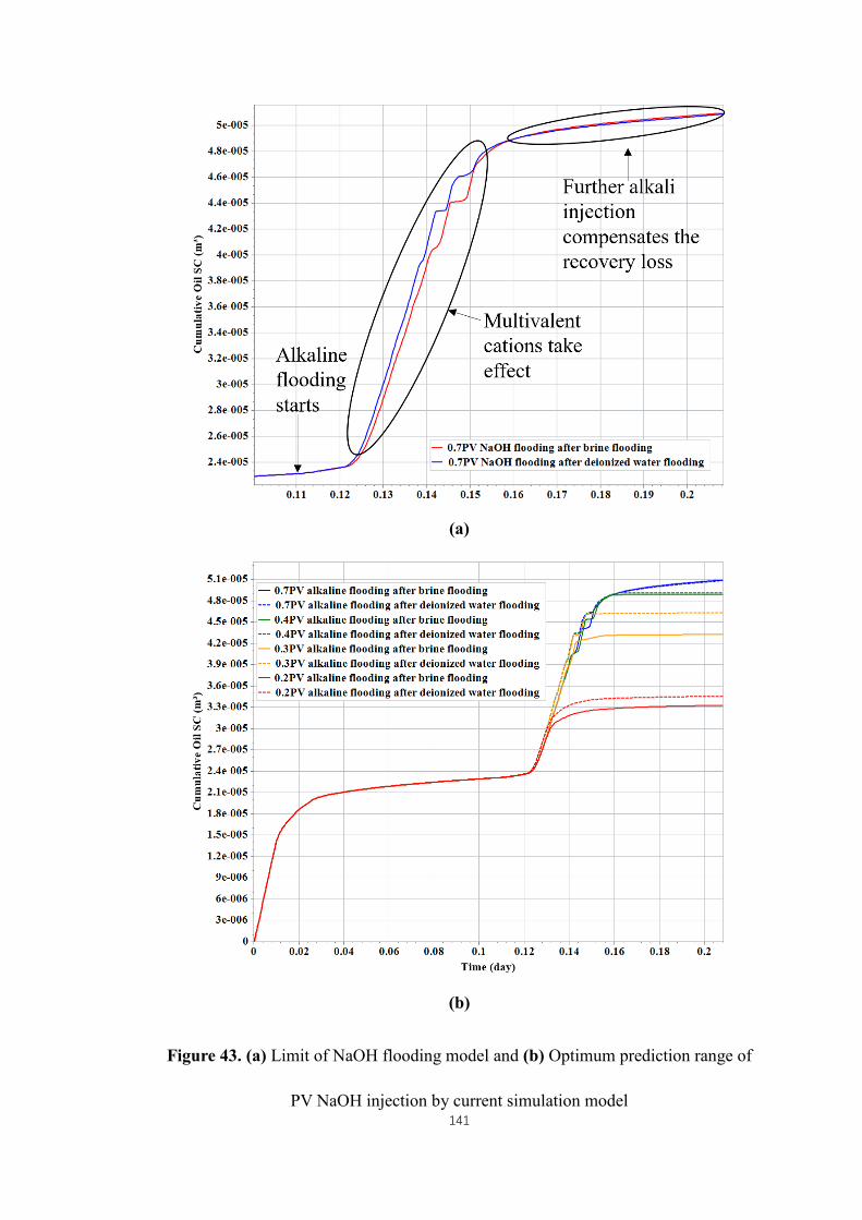
141
(a)
(b)
Figure 43. (a) Limit of NaOH flooding model and (b) Optimum prediction range of
PV NaOH injection by current simulation model

142
In reality, the injected alkaline solution goes into the water dominant channel at first
and react with the Ca2+ cation instantly. The system pH suddenly drops with solid
precipitation occurs. Due to the complexity of the saponification reaction, pH change
or ion occurrence is capable of alternating the in-situ surfactant generation types thus
affect the emulsification performance as well as the emulsion stability. The plugging
effect of the high viscous emulsion is crippled by the CaCl2 thus reduce the areal sweep
efficiency the NaOH injection should have achieved. Due to the depletion of carboxylic
acid in residual oil, more alkaline solution is wasted through the water dominating
channel than the deionized water case who enjoys the smooth and continuous
emulsification and plugging process. So, even at high PV NaOH injection, the real
cumulative oil recovery of flooding test should be less than the optimum condition
which is different from the simulation result. Current simulation model can be further
improved by building a 3D model to facilitate the water fingering during the flooding
process to make the model more representative. Besides, the multivalent cation effects
on the emulsification and emulsion stability is worth studying and additional
component reactions or models may be applied to the simulation to make the model
more physically accurate. For now, several comparison of oil recovery by brine model
and deionized model at various PV NaOH injection are plot in Figure 43(b). The eight
cases are divided into 4 groups by color based on the PV injection. The obvious
reduction of oil recovery due to the multivalent cation introduction is shown in 0.2 PV
and 0.3 PV alkaline injections. It can be concluded that the current model is still able
to be used to predict multivalent cation effect for PV NaOH injection lower than 0.3
PV, which is the optimum NaOH PV injection whose quantity required to produce
expected amount of oil is just fulfilled beyond this point.

143
Chapter 6: Conclusions and Recommendations
There are several conclusions can be drawn from the experiment and simulation results
which are listed in the following statements.
Firstly, sufficient shear force is significant for emulsion preparation. High shear mixer
like homogenizer which provides similar fluid channel configuration as sandpack
porous media is an ideal candidate in bottle test to successfully generate water in oil
emulsions. Secondly, the proposed modified bottle test is feasible for alkaline flooding
mechanism prediction as the major emulsion type determined by bottle test fully
matched the effluent emulsion type from flooding test. Besides, the emulsification and
entrapment mechanism plays the most effective role in oil recovery among other
alkaline flooding mechanisms. Such mechanism is mainly contributed by W/O
emulsion because of its extremely high viscosity and the large average water droplet
size which facilitates pore throat plugging. What is more, it is found that alkali type
selection is not the key to certain type of emulsion generation, but initial system’s [OH-]
concentration is. The emulsion type generated during alkaline flooding is not fixed but
interchangeable. W/O emulsion is more likely to occur under high [OH-] concentration
environment and vice versa. Weather in-situ surfactant with strong lipophilic or weak
lipophilic end is generated depend on the natural dissociation ability of alkalis, alkaline
concentration and environment temperature which consequently contributes to distinct
emulsion types that relate to different oil recovery mechanisms. Furthermore, brine
salinity effects on alkaline flooding rely on salt type. Monovalent cation generally
functions in moving the surfactants from aqueous phase to oil phase. So, alkaline
solution that introduces water in oil emulsion at initial stage is not sensitive to salinity
change. While emulsion type alteration is able to achieve if the original in-situ
surfactants introduced by alkaline solution reside in aqueous phase. On the contrary,

144
even small amount of multivalent cation deals great negative effects on alkaline
flooding performance as precipitation reaction directly consumes the inorganic alkali
quantity. In addition, the simulation model using reactions to represent essential
mechanisms of alkaline flooding have shown good prediction confidence at room
temperature. The prediction of emulsion production is the bonus of the enhanced
simulation model. What is more, according to the flooding test and simulation, the
optimum slug size of alkaline injection should be 0.3 PV. Last but not least, the preflush
operation requires 0.3 PV treated water to successfully reduce the brine salinity. Other
optimum alkaline concentration data was derived under ideal condition when deionized
water was used. These values are 0.02 mol/L for NaOH and 0.005 mol/L for Na2CO3
as references but actual value may vary depending upon reservoir brine salinity and
salt types.
As mentions, due to the design defect of the spinning drop tensiometer, IFT method
cannot provide correct optimum concentration for slow dissociation rate alkali. It is
recommended to use the tensiometer with dynamic sealing technology and advanced
balancing system to conduct dynamic IFT measurement. The IFT measurement should
be more representative to slow dissociation rate alkalis given enough reaction time.
The screening result will be better to collaborate IFT method with modified bottle test
to determine best combination of alkali concentration, salinity and temperature
according to different type of alkalis. What is more, further study of correlating the
homogenizing rate with the injection rate is recommended. By building the bridge
between the bottle test and sandpack flooding test, the representativeness of simulated
emulsification process in the bottle test can be enhanced. Moreover, as the modified
bottle test has been proved its feasibility in alkaline flooding mechanism prediction,
more studies regrading other types of alkalis, salts and temperature ranges can also be
145
conducted to further expand the utilization of the modified bottle test. As only two
inorganic alkalis and two salts were used in this research. The modified bottle test
including organic alkali, bio-alkali, newly synthesized alkali and brine water may lead
to a better illustration of current alkaline flooding development and closer relation to
the actual field. On the other hand, even though the alkaline simulation model provides
confident prediction for NaOH injection at room temperature, the high temperature
simulation does not provide satisfying results according to 70 ℃ flooding test. The
issue is targeted at the alkaline injection period because the simulated water flooding
performance is close to the sandpack flooding test. However, the response of oil
recovery to alkaline injection by simulation is delayed more than 2 hours. This is highly
possible that the saponification reaction rate calculated by CMG is not fast enough. It
is recommended to conduct the reaction rate measurement at higher temperature since
current Arrhenius equation is plotted based on 27~51 ℃ tests. The extrapolation of
higher temperature reaction rate may deviate as R2 of the Arrhenius equation is 0.88.
Besides, the emulsification reaction should be tuned as well regarding history data.
Therefore, there is still huge space of improvement for current reaction rate
measurement design as pH electrode has certain operating temperature limit. Other
advanced reaction rate instrument using titration method is suggested in this case. Last
but not least, the W/O emulsion viscosity and stability at various temperatures is
another point that worth studying and being considered by simulation.

146
REFERENCES
Acevedo, S., Escobar, G., Gutiérrez, L., & Rivas, H. (1992). Isolation and
characterization of natural surfactants from extra heavy crude oils, asphaltenes
and maltenes. Interpretation of their interfacial tension-pH behaviour in terms of
ion pair formation. Fuel, 71(6), 619-623.
Acevedo, S., Gutierrez, X., & Rivas, H. (2001). Bitumen-in-Water Emulsions
Stabilized with Natural Surfactants. Journal of Colloid and Interface Science,
242(1), 230-238.
Aminzadeh, B., Hoang, V., Inouye, A., Izgec, O., Walker, D., Chung, D., Dwarakanath,
V. (2016). Improving Recovery of a Viscous Oil Using Optimized Emulsion
Viscosity. SPE Improved Oil Recovery Conference.
Arhuoma, M., Dong, M., Yang, D., & Idem, R. (2009). Determination of Water-in-Oil
Emulsion Viscosity in Porous Media. Industrial & Engineering Chemistry
Research, 48(15), 7092-7102.
Arrhenius, S. A. (1889). "Über die Dissociationswärme und den Einfluß der
Temperatur auf den Dissociationsgrad der Elektrolyte". Z. Phys. Chem. 4: 96–116.
Ashrafizadeh, S., Motaee, E., & Hoshyargar, V. (2012). Emulsification of heavy crude
oil in water by natural surfactants. Journal of Petroleum Science and Engineering,
86-87, 137-143.
ASTM d6352-15, 2019, "Standard Test Method for Boiling Range Distribution of
Petroleum Distillates in Boiling Range from 174 °C to 700 °C by Gas
Chromatography" ASTM International.
Athreya, S. and Y.D. Venkatesh, 2012. Application of Taguchi method for optimization
of process parameters in improving the surface roughness of lathe facing
operation. Intl. Refereed J. Eng. Sci., 1:13-19.
147
Baek, K. H., Argüelles-Vivas, F. J., Okuno, R., Sheng, K., Sharma, H., & Weerasooriya,
U. P. (2018). Organic Alkali as a Steam Additive for Improved SAGD:
Experimental Study of Emulsion Phase Behavior and Viscosity. SPE Canada
Heavy Oil Technical Conference.
Barroso-Solares, S., Pinto, J., Nanni, G., Fragouli, D., & Athanassiou, A. (2018).
Enhanced oil removal from water in oil stable emulsions using electrospun
nanocomposite fiber mats. RSC Advances, 8(14), 7641-7650.
Blunt, Martin J. (2017) “Multiphase Flow in Permeable Media by Martin J. Blunt.”
Cambridge Core, Cambridge University Press.
Bryan, J. L., & Kantzas, A. (2007). Enhanced Heavy-Oil Recovery by Alkali-
Surfactant Flooding. SPE Annual Technical Conference and Exhibition.
Chhabra R.P., Richardson J.F., in Non-Newtonian Flow in the Process Industries, 1999
CMG, Stars User Guide: Advanced Processes & Thermal Reservoir Simulation, 2015
Cooke, C., Williams, R., & Kolodzie, P. (1974). Oil Recovery by Alkaline
Waterflooding. Journal of Petroleum Technology, 26(12), 1365-1374.
Dehghan, A. A., Masihi, M., & Ayatollahi, S. (2013). Evaluation of Chemicals
Interaction with Heavy Crude Oil through Water/Oil Emulsion and Interfacial
Tension Study. Energy & Fuels, 27(10), 5852-5860.
Dhankhar, P. (2014). Homogenization Fundamentals. IOSR Journal of Engineering,
4(5), 01-08.
Ding, B., Zhang, G., Ge, J., & Liu, X. (2010). Research on Mechanisms of Alkaline
Flooding for Heavy Oil. Energy & Fuels, 24(12), 6346-6352.
Dong, M., Liu, Q., & Li, A. (2012). Displacement mechanisms of enhanced heavy oil
recovery by alkaline flooding in a micromodel. Particuology, 10(3), 298-305.

148
Ersoy, Gizem, et al. “Modeling of Inversion Point for Heavy Oil-Water Emulsion
Systems.” SPE Annual Technical Conference and Exhibition, 2008.
Ezzati, A., Gorouhi, E., & Mohammadi, T. (2005). Separation of water in oil emulsions
using microfiltration. Desalination, 185(1-3), 371-382.
Ge, J., Feng, A., Zhang, G., Jiang, P., Pei, H., Li, R., & Fu, X. (2012). Study of the
Factors Influencing Alkaline Flooding in Heavy-Oil Reservoirs. Energy & Fuels,
26(5), 2875-2882.
Green, Don W., and G. Paul Willhite. Enhanced Oil Recovery. Society of Petroleum
Engineers, 2018.
Guo, H., Li, Y., Wang, F., Yu, Z., Chen, Z., Wang, Y., & Gao, X. (2017). ASP Flooding:
Theory and Practice Progress in China. Journal of Chemistry, 2017, 1-18.
Homsy, G. (1987). Viscous Fingering In Porous Media. Annual Review of Fluid
Mechanics, 19(1), 271-311.
“IR Spectrum Table & Chart.” Sigma, https://www.sigmaaldrich.com/technical-
documents/articles/biology/ir-spectrum-table.html.
Johnson, C. (1976). Status of Caustic and Emulsion Methods. Journal of Petroleum
Technology, 28(01), 85-92.
Kokal, S.; Abdulaziz, A. Enhanced Oil Recovery: Challenges and Opportunities.
InWorld Petroleum Council: Global Energy Solutions; World Petroleum Council:
London, UK, 2010; pp. 64–69.
Mayer, E H, et al. “Alkaline Injection for Enhanced Oil Recovery - A Status Report.”
Society of Petroleum Engineering of AIME, Jan. 1983, pp. 209–221.
Nagarajan, N. R., Dong, C., Mullins, O. C., & Honarpour, M. M. (2012). Challenges
of Heavy Oil Fluid Sampling and Characterization. SPE Annual Technical
Conference and Exhibition.
149
Nelson, R., Lawson, J., Thigpen, D., & Stegemeier, G. (1984). Cosurfactant-Enhanced
Alkaline Flooding. Proceedings of SPE Enhanced Oil Recovery Symposium.
“Oil Resources.” Natural Resources Canada, 25 July 2017,
https://www.nrcan.gc.ca/energy/energy-sources-distribution/crude-oil/oil-
resources/18085.
Panthi, K., & Mohanty, K. K. (2013). Effect of Alkaline Preflush in an Alkaline-
Surfactant-Polymer Flood. Energy & Fuels, 27(2), 764-771
Pei, H., Zhang, G., Ge, J., Tang, M., & Zheng, Y. (2012). Comparative Effectiveness
of Alkaline Flooding and Alkaline–Surfactant Flooding for Improved Heavy-Oil
Recovery. Energy & Fuels, 26(5), 2911-2919.
Pitts, M.J., Wyatt, K., and Surkalo, H. “Alkaline-Polymer Flooding of the David Pool,
Lloydminster Alberta.” Proceedings of SPE/DOE Symposium on Improved Oil
Recovery, 2004
Rivas, H., Gutierrez, X., Zirrit, J. L., Anto'n, R. E. & Salager, J. L. 1997.
“Microemulsion and optimum formulation occurrence in pH dependent systems
as found in alkaline enhanced oil recovery”. In Industrial Applications of
Microemulsions Edited by: Solans, C. and Kunieda, H. 305–329. New York: M.
Dekker.
Shao, S., Li, X., Pang, L., & Ma, L. (jun. 2004). Measurement of Rate Constant for
Saponification Reaction of Ethyl Acetate by Acidometer. Journal of Xi`an
University of Science and Technology, 24(2), 196-199.
Sun, J., Sun, L., Liu, W., Liu, X., Li, X., & Shen, Q. (2008). Alkaline consumption
mechanisms by crude oil: A comparison of sodium carbonate and sodium
hydroxide. Colloids and Surfaces A: Physicochemical and Engineering Aspects,
315(1-3), 38-43.

150
Sun, N., Jing, J., Jiang, H., An, Y., Wu, C., Zheng, S., & Qi, H. (2017). Effects of
Surfactants and Alkalis on the Stability of Heavy-Oil-in-Water Emulsions. SPE
Journal, 22(01), 120-129.
Wang, J., Dong, M., & Arhuoma, M. (2010). Experimental and Numerical Study of
Improving Heavy Oil Recovery by Alkaline Flooding in Sandpacks. Journal of
Canadian Petroleum Technology, 49(03), 51-57.
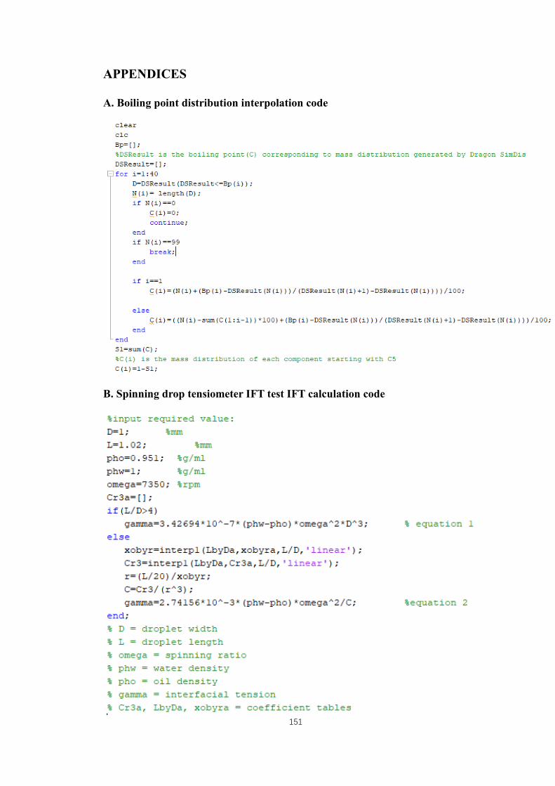
151
APPENDICES
A. Boiling point distribution interpolation code
B. Spinning drop tensiometer IFT test IFT calculation code