an experimental investigation of the mechanism of heat
TRANSCRIPT

An Experimental Investigation of the Mechanism of Heat Transfer Augmentation by Coherent Structures
David Owen Hubble
A dissertation submitted to the faculty of the Virginia Polytechnic Institute and State University in partial
fulfillment of the requirements for the degree of
Doctor of Philosophy
in
Mechanical Engineering
Virginia Tech Department of Mechanical EngineeringAdvanced Experimental Thermofluids Research Laboratory
Thomas Diller, ChairmanPavlos Vlachos, Co Chairman
Roger SimpsonClinton DanceyScott HuxtableMark Stremler
02.08.2011Blacksburg, Virginia
Keywords: heat transfer, mechanism, turbulence, heat flux sensor, particle image velocimetry, timeresolved, vortex
Copyright 2011, David O. Hubble

An Experimental Investigation of the Mechanism of Heat Transfer Augmentation by Coherent Structures
David Owen Hubble
Abstract
The mechanism by which convective heat transfer is augmented by freestream turbulence in the
stagnation region was studied experimentally. Previous work has suggested that the primary mechanism
for the observed augmentation is the amplification of vorticity into strong vortices which dominate the
flow field near the surface. Therefore, two separate experimental investigations were performed to
further study this phenomenon. In the first, the spatiotemporal convection from a heated surface was
measured during the normal collision of a vortex ring. The convection was observed to increase
dramatically in areas where vortices forced outer fluid through the natural convection boundary layer to
the surface. Regions where fluid was swept along the surface experienced much smaller increases in
convection. These observations led to the development of a mechanistic model which predicted the
heat transfer based on the amount of time that fluid remained within the thermal boundary layer prior
to reaching the surface. In subsequent testing, the model was able to accurately predict the time
resolved convection based solely on the transient properties of the vortex present. In the second
investigation, the model was applied to the vortices which form in a stagnating turbulent flow. Three
turbulence conditions were tested which changed the properties of the vortices produced. Again, the
model was successful in predicting the time resolved convection over much of the experimental
measurement time.
The work of designing and calibrating the heat flux sensor used is also reported. A new sensor was
developed specifically for the convection research performed herein as no existing sensor possessed the
required spatiotemporal resolution and underwater capabilities. Utilizing spot welded foils of
thermoelectric alloys resulted in a very robust and sensitive sensing array which was thoroughly
analyzed and calibrated. In the final section, the hybrid heat flux (HHF) method is presented which
significantly increases the performance of existing heat flux sensors. It is shown (both numerically and
experimentally) that by combining the spatial and temporal temperature measurements from a
standard sensor, the time response increases by up to a factor of 28. Also, this method causes the
sensor to be insensitive to the material to which it is mounted.
Acknowledgements
There are a number of people who have helped me reach my goal of obtaining a PhD in mechanical
engineering. First, my research advisors Dr. Tom Diller and Dr. Pavlos Vlachos deserve recognition. You
have taught me how to be a successful researcher but more importantly how to be a professional. Your
guidance is deeply appreciated. Also, to my dissertation committee I give a sincere thank you for your
help guiding this research.
No one has helped in this research more than my fellow AEThER lab mates. In particular I thank my
collaborators Andrew Gifford, Clayton Pullins, Arun Mangalam, and Jerrod Ewing. I have also worked
closely with a number of other lab mates including Christopher Weiland, Satya Karri, Nick Cardwell,
Kelley Stewart, Dave Griffiths, Sam Raben, John Charonko, the list goes on and on. I really enjoyed are
time together and hope that we can work together again in the future.
Several members of the Randolph Hall staff deserve special recognition for their help. The ladies of
the ME office have helped me out of many jams with special thanks to Cathy Hill, Diana Isreal, and
Renee Shack. A special thanks also goes out to the ME machine shop and Bill Songer in particular for
always tolerating my requests for him to machine inconel.
My family has been very supportive of this endeavor and my life long goal of being an engineer. No
one has taught me more about engineering than my dad. My mom always pushed me to do my best and
to her education is everything. For instilling in me this love of learning I say thank you.
Lastly I thank Samantha for putting our life together on hold while I pursue this degree. Thanks for
bringing me supper 12 hours into a 24 hour test and putting up with me going back to work after
supper. I wouldn’t have been able to do this without your support.

iv
Table of Contents
Abstract............................................................................................................................... ...................... ii
Acknowledgements............................................................................................................................... ... iii
List of Figures ............................................................................................................................... .......... viii
List of Tables ............................................................................................................................... ............. xi
1 Introduction ..................................................................................................................... 1
1.1 Motivation............................................................................................................................... ...... 1
1.2 Objective and Structure of Dissertation ....................................................................................... 1
2 A Mechanistic Model for the Convection Caused by Coherent Structures: Examining a
Vortex Ring Collision with a Surface ........................................................................................ 4
2.1 Abstract ............................................................................................................................... .......... 4
2.2 Nomenclature ............................................................................................................................... 4
2.3 Introduction ............................................................................................................................... ... 5
2.4 Experimental Measurements........................................................................................................ 7
2.4.1 Vortex Ring Generator. ......................................................................................................... 8
2.4.2 Instrumented Flat Plate ........................................................................................................ 9
2.4.3 Flow Measurements: Time Resolved Particle Image Velocimetry ..................................... 11
2.4.4 Vortex identification and circulation calculation ................................................................ 12
2.4.5 Steady properties of the heated surface ............................................................................ 13
2.5 Ring impingement and resulting heat transfer........................................................................... 14
2.6 A Mechanistic Model .................................................................................................................. 17
2.6.1 A time resolved model........................................................................................................ 17
2.7 Comparison of the analytical model and experimental results .................................................. 20
2.8 Conclusions ............................................................................................................................... ..24

v
3 A Mechanistic Model of Turbulent Heat Transfer Augmentation in Stagnation Flow...... 26
3.1 Abstract ............................................................................................................................... ........ 26
3.2 Nomenclature ............................................................................................................................. 26
3.3 Introduction ............................................................................................................................... .27
3.4 Mechanistic Model...................................................................................................................... 28
3.5 Experimental Methodology ........................................................................................................ 30
3.5.1 Water Tunnel Facility and Turbulence Generation............................................................. 31
3.5.2 Instrumented Flat Plate ...................................................................................................... 32
3.5.3 Flow Measurements: Time Resolved Particle Image Velocimetry ..................................... 32
3.5.4 Vortex identification ........................................................................................................... 32
3.6 Experimental Measurements...................................................................................................... 32
3.6.1 Laminar Baseline ................................................................................................................. 32
3.6.2 Transient Flow and Convection: Physical Insight of the Mechanism.................................. 33
3.7 Comparison of the analytical model and experimental results .................................................. 35
3.8 Conclusions ............................................................................................................................... ..40
3.9 Acknowledgements..................................................................................................................... 40
4 Development and Evaluation of the Time Resolved Heat and Temperature Array ......... 41
4.1 Abstract ............................................................................................................................... ........ 41
4.2 Nomenclature ............................................................................................................................. 41
4.3 Introduction ............................................................................................................................... .42
4.4 Sensor Design.............................................................................................................................. 44
4.5 Sensor Fabrication ...................................................................................................................... 45
4.6 Theoretical Sensitivity and Time Response ................................................................................ 46
4.7 Sensor Calibration ....................................................................................................................... 49
4.7.1 Seebeck Coefficient Measurement..................................................................................... 49

vi
4.7.2 Conduction Calibration ....................................................................................................... 50
4.7.3 Radiation Calibration .......................................................................................................... 53
4.7.4 Hybrid Heat Flux Analysis.................................................................................................... 57
4.7.5 Calibration Summary........................................................................................................... 58
4.8 Example of Sensor Application ................................................................................................... 59
4.8.1 Steady Convection .............................................................................................................. 59
4.8.2 Unsteady Convection .......................................................................................................... 60
4.9 Uncertainty Analysis ................................................................................................................... 61
4.10 Conclusions ............................................................................................................................... ..63
4.11 Acknowledgments....................................................................................................................... 63
5 A Hybrid Method for Heat Flux Measurement................................................................ 64
5.1 Abstract ............................................................................................................................... ........ 64
5.2 Nomenclature ............................................................................................................................. 64
5.3 Introduction ............................................................................................................................... .65
5.4 Background ............................................................................................................................... ..65
5.5 HHF Methodology ....................................................................................................................... 68
5.5.1 Differential Term................................................................................................................. 68
5.5.2 Slug Term ............................................................................................................................ 70
5.5.3 Hybrid Heat Flux.................................................................................................................. 71
5.6 HHF Numerical Validation........................................................................................................... 73
5.7 HHF Experimental Validation ...................................................................................................... 77
5.8 Conclusions ............................................................................................................................... ..83
5.9 Acknowledgments....................................................................................................................... 83
6 Conclusions and Recommendations for Future Work ..................................................... 84
6.1 Conclusions ............................................................................................................................... ..84

vii
6.2 Recommendations for Future Research ..................................................................................... 85
7 Appendix ........................................................................................................................ 87
7.1 Experimental details of the vortex ring experiment................................................................... 87
7.2 Details of the fabrication of the THeTA ...................................................................................... 87
7.3 Experimental validation of the HHF method .............................................................................. 89
7.4 Computational codes .................................................................................................................. 90
7.4.1 Vortex ring analysis ............................................................................................................. 90
7.4.2 Stagnating flow analysis...................................................................................................... 95
7.4.3 Simulation of heat flux sensors......................................................................................... 103
7.5 References ............................................................................................................................... .107
7.6 Copyright Transfer Material...................................................................................................... 111

viii
List of Figures
*Unless otherwise noted, all images are the property of the author
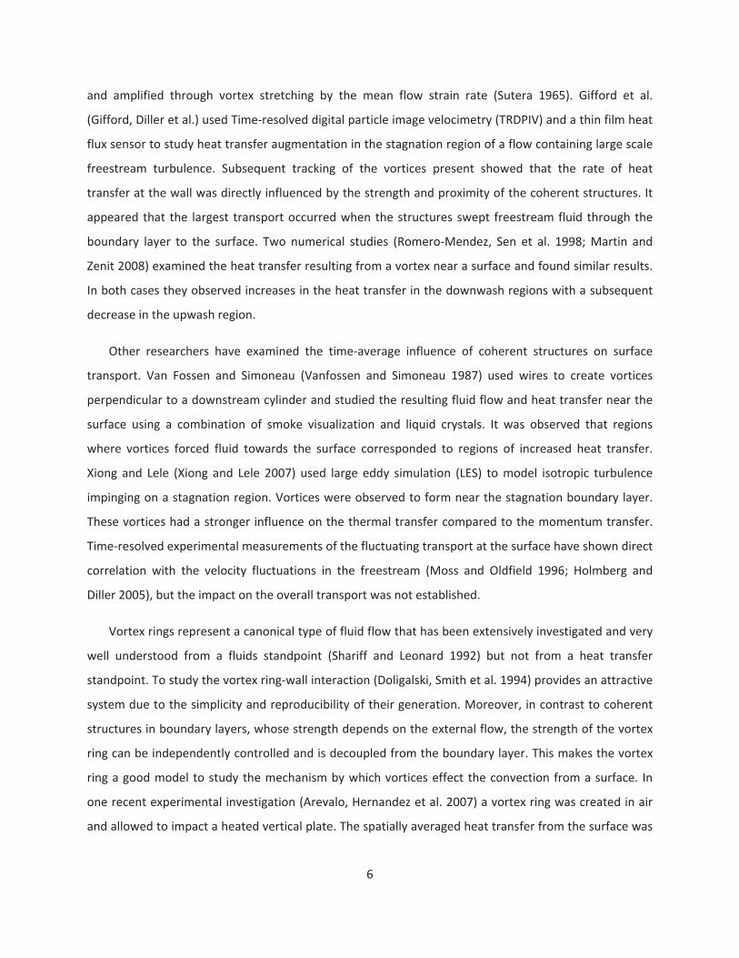
FIG. 2.1WATER TUNNEL FACILITY AND EXPERIMENTAL SETUP .....................................................................................................8
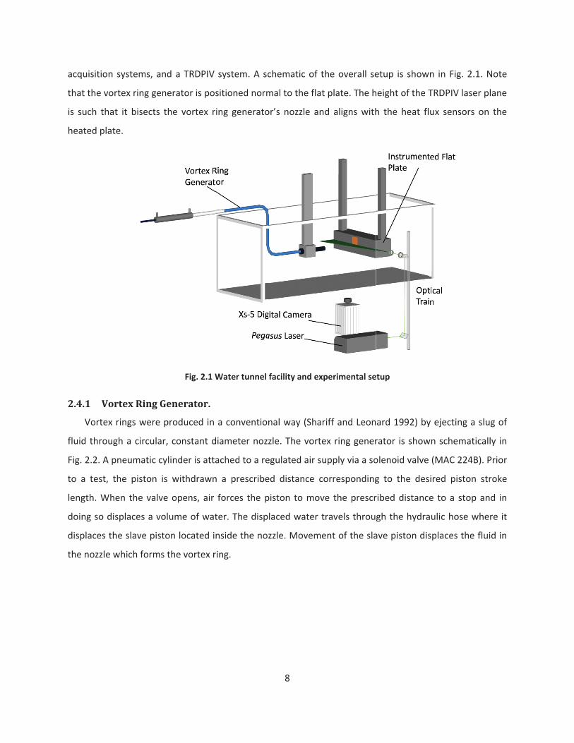
FIG. 2.2 SCHEMATIC OF VORTEX RING GENERATOR.................................................................................................................... 9
FIG. 2.3 FLAT PLATE MODEL AND INSTRUMENTATION ..............................................................................................................10
FIG. 2.4 THE TIME RESOLVED HEAT AND TEMPERATURE ARRAY (THETA). PROVIDES A MEASURE OF BOTH HEAT FLUX AND SURFACE
TEMPERATURE AT 10 LOCATIONS. ............................................................................................................................... 11
FIG. 2.5 NON DIMENSIONAL BOUNDARY LAYER PROFILE SHOWNWITH STANDARD SCALING.............................................................14
FIG. 2.6 ILLUSTRATION OF RING IMPINGEMENT AND HEAT TRANSFER. VELOCITY FIELDS SEQUENCE AT LEFT REPRESENT ONE HALF OF THE
VORTEX RING OVER A ONE HALF SECOND PERIOD. AS THE RING APPROACHES THE HEATED PLATE THE MEASURED CONVECTION
INCREASES AS ILLUSTRATED AT RIGHT. MARKERS IN THE VELOCITY FIELDS CORRESPOND TO INDIVIDUAL HEAT FLUX SENSOR LOCATIONS
AND INDICATE THE TIMING AT RIGHT. ........................................................................................................................... 16
FIG. 2.7 CLOSE UP OF INTERACTION PROCESS AND MEASURED RATE OF CONVECTION. THE SENSORS IN THE DOWNWASH REGION OF THE
VORTEX EXPERIENCE MORE CONVECTION THAN THE SENSOR DIRECTLY BENEATH THE VORTEX AND MUCH MORE CONVECTION
COMPARED TO SENSORS IN THE UPWASH REGION. ..........................................................................................................17
FIG. 2.8 SCHEMATIC USED IN MODEL DEVELOPMENT ALONGWITH FUNCTIONAL MODEL RESULTS. MODEL PREDICTS MUCH LARGER
CONVECTION IN THE DOWNWASH REGION COMPARED TO THE UPWASH REGION DUE TO THE SHORTER VALUE OF DBA COMPARED TO
DBC. ............................................................................................................................... .......................................18
FIG. 2.9MEASURED CIRCULATION OF VORTEX AS IT APPROACHES THE PLATE FOR THREE DIFFERENT TESTS. THE CIRCULATION IS USED TO
CALCULATE THE INDUCED VELOCITY AT THE SENSOR LOCATION ON THE PLATE USING THE BIOT SAVART LAW...............................21
FIG. 2.10 THE DISTANCE THAT FLUID MUST TRAVEL WITHIN THE THERMAL BOUNDARY LAYER (DBA,+) IS CALCULATED FROM THE MEASURED
VORTEX LOCATION. COMBING THIS VALUE WITH THE INDUCED VELOCITY FROM ABOVE YIELDS THE CHARACTERISTIC TIME ( , ) USED
IN THE MODEL. RE =5800............................................................................................................................... ..........22
FIG. 2.11 COMPARISON OF MODEL PREDICTION TO MEASURED CONVECTION DURING VORTEX INTERACTION. RESULTS SHOWN FROM THREE
REPRESENTATIVE TESTS SPANNING THE RANGE OF VORTEX STRENGTHS. ...............................................................................23
FIG. 2.12 COMPARISON OF THE MAXIMUMMEASURED CONVECTION WITH MAXIMUMMODEL PREDICTION FOR THE RANGE OF TEST
CONDITIONS. THE DOTTED LINES REPRESENT THE + 15% BOUNDS. ....................................................................................24
FIG. 3.1 SCHEMATIC USED IN MODEL DEVELOPMENT WITH FUNCTIONAL MODEL RESULTS. MODEL PREDICTS LARGER CONVECTION IN THE
DOWNWASH REGION DUE TO THE SHORTER DISTANCE THAT FLUID TRAVELS WITHIN THERMAL BOUNDARY LAYER. ........................30
FIG. 3.2WATER TUNNEL FACILITY AND POSITION OF MODEL RELATIVE TO TURBULENCE GRID AND TRDPIV SYSTEM.............................31
FIG. 3.3 INSTANTANEOUS SNAP SHOT OF THE FLOW FIELD AND CONVECTION. SENSOR LOCATIONS ARE INDICATED BY THE BLACK DOTS AND
CONVECTION MEASUREMENTS ARE GIVEN BY THE BARS AT RIGHT. THE CONTOUR OF THE VECTOR FIELD SHOWS THE MAGNITUDE OF
THE U VELOCITY. CONVECTION INCREASES ARE LOCALIZED TO AREAS OF VORTEX DOWNWASH. ................................................34

ix
FIG. 3.4 TRANSIENT INTERACTION OF A SINGLE VORTEX WITH THE SURFACE AND RESULTING CONVECTION. VORTEX LOCATION AND
STRENGTH ARE INDICATED BY THE CIRCULAR MARKERS AT LEFT WHILE THE COLOR CORRESPONDS TO THE TIME AT RIGHT. CONVECTION
HISTORY FOR THREE NEARBY SENSOR LOCATIONS IS SHOWN. .............................................................................................35
FIG. 3.5 THREE VORTEX TRACKS AND RESULTING MEASURED CONVECTION.MARKER SIZE INDICATES RELATIVE STRENGTH (CIRCULATION) OF
VORTEX WHILE THE FILL COLOR CORRESPONDS TO THE TIME AS INDICATED AT RIGHT WHERE THE MEASURED CONVECTION IS SHOWN.
............................................................................................................................... .............................................36
FIG. 3.6 TRANSIENT PROPERTIES OF THE THREE VORTICES DURING THE INTERACTION TIME ..............................................................37
FIG. 3.7 TRANSIENT MODEL INPUTS DERIVED FROM VORTEX PROPERTIES .....................................................................................38
FIG. 3.8MODEL PREDICTION WITH MEASURED CONVECTION. THE SHADED REGION CORRESPONDS TO THE 3.5 SECONDS STUDIED IN DETAIL
IN THE PREVIOUS THREE FIGURES. ............................................................................................................................... .39
FIG. 4.1 CONCEPTUAL DESIGN OF THE THETA. THE TEMPERATURE DROP IS PROPORTIONAL TO V1 AND THE SURFACE TEMPERATURE IS
INDICATED BY V2............................................................................................................................... .....................45
FIG. 4.2 THETA DURING CONSTRUCTION. SPOT WELDED THERMOELECTRIC FOILS ARE FOLDED OVER KAPTON RESISTANCE BARRIER........46
FIG. 4.3 COMPLETED THETAWIRE FOR 10 HEAT FLUX AND SURFACE TEMPERATURE MEASUREMENTS ..............................................46
FIG. 4.4 CROSS SECTIONAL VIEW OF THETA AND ITS ELECTRICAL ANALOGY..................................................................................48
FIG. 4.5 STEADY STATE CONDUCTION CALIBRATION FACILITY. HEAT FLUX IS MAINTAINED BETWEEN THE UPPER HEATED PALTE AND THE
LOWER COOLED PLATE................................................................................................................................ ...............51
FIG. 4.6 CONDUCTION CALIBRATION RESULTS WITH 95% CONFIDENCE UNCERTAINTY AND THEORETICAL PREDICTION...........................52
FIG. 4.7 SENSITIVITY DEPENDENCE ON SENSOR THICKNESS ........................................................................................................53
FIG. 4.8 LAMP RADIATION INTENSITY AS A FUNCTION OF RADIAL LOCATION..................................................................................54
FIG. 4.9 RADIATION CALIBRATION SETUP. SHUTTER UTILIZED TO PROVIDE A STEP CHANGE IN INCIDENT FLUX.......................................55
FIG. 4.10 RADIATION CALIBRATION RESULTS WITH 95% CONFIDENCE UNCERTAINTY AND THEORETICAL PREDICTION ............................55
FIG. 4.11 TRANSIENT RESPONSE OF THETA TO STEP RADIATION HEAT FLUX INPUT ........................................................................56
FIG. 4.12 TIME RESPONSE OF THE LOGARITHMIC HEAT FLUX AND LEAST SQUARES FIT. FIT USED TO MEASURE FIRST ORDER TIME CONSTANT
............................................................................................................................... .............................................57
FIG. 4.13 HYBRID HEAT FLUX RESPONSE OF THETA TO STEP CHANGE INPUT COMPARED TO DIFFERENTIAL RESPONSE ...........................58
FIG. 4.14 SETUP FOR CONVECTION ANALYSIS. HIEMENZ FLOW PRODUCED IN A WATER TUNNEL FACILITY............................................60
FIG. 4.15 COMPARISON OF MEASURED AND PREDICTED HEAT TRANSFER COEFFICIENT VALUES. ........................................................60
FIG. 4.16 SENSOR APPLICATION, VORTEX RING IMPINGING ON A HEATED PLATE. ...........................................................................61
FIG. 5.1 SENSOR BACKING SYSTEM. T1 AND T2 ARE THE TWO SENSOR SURFACE TEMPERATURES.......................................................66
FIG. 5.2 INSTANTANEOUS TEMPERATURE PROFILE WITHIN SENSOR BACKING SYSTEM. ....................................................................69
FIG. 5.3 COMPARISON OF SLUG CALORIMETER RESPONSE USING DIFFERENT SENSOR TEMPERATURE MEASUREMENTS. ..........................71
FIG. 5.4 SIMULATED RESPONSE OF SENSOR IN THREE MODES OF OPERATION. HHF METHOD SIGNIFICANTLY INCREASES SENSOR
PERFORMANCE. ............................................................................................................................... ........................74
FIG. 5.5 ERROR AS A FUNCTION OF TIME AND BACKING MATERIAL THERMAL CONDUCTIVITY FOR THREE MODES OF SENSOR OPERATION. ..75

x
FIG. 5.6 ERROR OF HHF2 USING ONLY T2 IN SLUG CALORIMETER TERM OF HHF COMPARED WITH STANDARD METHODS. .....................76
FIG. 5.7 ERROR OF HHF1 USING ONLY T1 IN SLUG CALORIMETER TERM OF HHF COMPARED WITH STANDARD METHODS. .....................77
FIG. 5.8 HTHFS DESIGN OVERVIEW. THERMOPILE USE TO MEASURE TEMPERATURE DROP ACROSS CALIBRATED THERMAL RESISTANCE. ...78
FIG. 5.9 STAGNATION FLOW CONVECTION CALIBRATION FACILITY. T NOZZLE PRODUCES SYMMETRIC STAGNATING JETS ON TEST SENSOR
AND REFERENCE SENSOR................................................................................................................................ ............79
FIG. 5.10 CONVECTIVE HEAT TRANSFER COEFFICIENT MEASURED BY THE HFM REFERENCE SENSOR. .................................................80
FIG. 5.11 SENSOR RESPONSE ON WATER COOLED BACKING WITH APPLIED FLUX SHOWN. ................................................................81
FIG. 5.12 SENSOR ON WATER COOLED BACKING USING ONLY T2 IN SLUG AND HYBRID METHODS. .....................................................81
FIG. 5.13 SENSOR RESPONSE MOUNTED ON A THERMAL INSULATOR WITH APPLIED FLUX SHOWN. ....................................................82
FIG. 5.14 SENSOR ON INSULATED BACKING USING ONLY T2 IN SLUG AND HYBRID METHODS.............................................................83
FIG. 7.1 DIFFERENTIAL, SLUG, AND HHF RESPONSE OF SENSOR TO STEP RADIATION FLUX. RESULTS OF 6 TESTS OVERLAID AND NORMALIZED
BY THE APPLIED HEAT FLUX. ............................................................................................................................... .........90

xi
List of Tables
TABLE 3.1 DETAILS OF GRIDS AND TURBULENCE STATISTICS.......................................................................................................31
TABLE 3.2 SUMMARY OF TIME AVERAGED AUGMENTATION AND MODEL PREDICTIONS...................................................................39
TABLE 4.1 SUMMARY OF THETA CALIBRATION RESULTS...........................................................................................................58
TABLE 5.1 PARAMETERS USED IN NUMERICAL SIMULATION .......................................................................................................73
TABLE 7.1 SUMMARY OF TEST CONDITIONS USED IN VORTEX RING EXPERIMENT ............................................................................87

1
1 Introduction
1.1 MotivationFreestream turbulence has a major effect on surface heat transfer which influences many
engineering applications, for example, gas turbines, combustors, electronic cooling devices, and heat
exchangers. Numerous studies have shown that elevated freestream turbulence levels cause an increase
in the time averaged heat transfer over laminar flow levels. Modeling this augmentation in such
circumstances is difficult even for simple flows and geometries because of the unpredictable effect of
the freestream turbulence. The mechanism by which this augmentation takes place must be understood
if an accurate predictive tool is to be produced. In this work, new experimental techniques are
developed and utilized to gain a deeper understanding of this complicated mechanism.
1.2 Objective and Structure of DissertationThe objective of this dissertation is to provide an understanding of the mechanism by which
convective heat transfer is augmented by freestream turbulence in stagnating flows. To accomplish this,
four separate but related studies were undertaken and therefore this dissertation is broken into four
sections. The following gives a brief introduction to the work performed while each individual chapter
gives a more thorough introduction to the specific subject matter.
A number of researchers have performed experiments which suggest that the primary mechanism
for the augmentation of heat transfer by freestream turbulence is the formation of strong vortices
which dominate the flow field near the surface. Therefore, this investigation begins by attempting to
determine the convection caused by an easily controlled vortex. Chapter 2 reports an experiment in
which a vortex ring is produced and allowed to collide normally with a heated instrumented surface.
Two time resolved measurements technologies are exploited to quantitatively visualize the interaction.
Specifically, time resolved digital particle image velocimetry (TRDPIV) is used to investigate the time
resolved flow structure during the interaction while a time resolved heat and temperature array
(THeTA) is used to map the convective heat transfer coefficient at the surface. These measurements
provide valuable insight into the mechanism by which vortices affect the heat transfer from a surface.
These measurements lead to the development of a mechanistic model which is then used to predict the
time resolved convection based only on the transient properties of the vortex. Results are presented for
a range of vortex parameters.

2
In chapter 3, the model developed in chapter 2 is applied to a flow that is more relevant from an
engineering standpoint. Here the stagnation region is examined in a flow which contains large scale
freestream turbulence. Again, TRDPIV is used in conjunction with a THeTA to examine the interaction
process. In the stagnation region, properly oriented and scaled freestream structures are amplified into
strong vortices which dominate the flow field near the surface. These vortices cause large spikes in heat
transfer and as a result cause an overall increase in the time average convection. Results are presented
which shows the behavior of the vortices that form along with the simultaneously measured convection.
Also, results are presented which show how the model can be applied to these complicated flow fields
to obtain accurate, time resolved convection predictions.
The work of developing and evaluating the THeTA is presented in chapter 4. While this sensor is
similar to existing sensors, it is of totally new design using spot welded thermoelectric foils to measure
both the surface temperature of the sensor as well as the temperature drop across the sensor.
Analytical and numerical modeling was performed to estimate the time response and sensitivity of the
sensor. Calibrations were then performed applying both conductive and radiative heat fluxes to
measure the sensitivity and time response. A test of the sensor’s response in convection is also
presented. The resulting gage should be a valuable tool for convection research as it can directly
measure the time resolved heat transfer coefficient at multiple locations simultaneously.
Chapter 5 reports the development of the hybrid heat flux (HHF) method for obtaining heat flux
measurements. In this method, both the spatial and temporal temperature measurements of
differential style heat flux sensors are used. By using both measurements, both the heat flowing through
the gage as well as the heat being absorbed by the gage is accounted for. It is shown that this improves
the time response of the sensor by up to a factor of 28 compared to utilizing the spatial measurements
alone as is the standard practice. Perhaps more importantly, utilizing the hybrid method renders the
sensor essentially insensitive to the material to which it is mounted. Traditionally, sensors must be
mounted on a good thermal conductor for accurate measurements to be made which didn’t allow their
use on insulation. It is shown that when using the hybrid method, changing the thermal conductivity of
the backing material four orders of magnitude causes only an 11% change in sensor output. Results are
presented from both numerical and experimental testing of a sensor utilizing the HHF method. The
signals from the THeTA in chapters 2 and 3 were also vastly improved by utilizing the HHF method.

3
The individual chapters (2 5) are presented in a journal manuscript format as each has or will be
submitted to archival journals for publication. Chapters 2 and 3 have not yet been submitted. Chapter 4
has been published in the ASME Journal of Thermal Science and Engineering Application and chapter 5
has been published in the ASME Journal of Heat Transfer.

4
2 A Mechanistic Model for the Convection Caused by Coherent
Structures: Examining a Vortex Ring Collision with a Surface
David O. Hubble, Pavlos P. Vlachos, and Tom E. Diller
2.1 AbstractThe physical mechanism by which coherent structures influence the convective heat transfer from a
surface is a basic problem of fluid mechanics which plays a central role turbulence. To explore this
phenomena, a well defined structure (specifically a vortex ring) was generated which impacted a heated
instrumented surface while the time resolved characteristics of the flow field were measured. By
examining both the heat transfer and flow field in a time resolved fashion, it was observed that the
surface transport was driven by the sweeping of fluid through the boundary layer by this large scale
vortex structure. A physics based mechanistic model was developed from the experimental
observations which predicts the time resolved surface convection using the transient properties of the
coherent flow structure. The model was shown to predict the measured convection in a majority of the
tests spanning circulation Reynolds numbers from 3100 to 9200. These results indicate the central role
of large scale structures in the augmentation of thermal transport and give a simple approach for
quantitative prediction.
2.2 Nomenclature = thermal diffusivity (m2/s)
= thermal expansion coefficient (1/K)
C = specific heat (J/kg K)
d = distance (m)
D = slave piston diameter (m)
= boundary layer thickness (m)
g = gravitational constant
G = Grashof number
= circulation (m2/s)
h = convective heat transfer coefficient (W/m2 K)
k = thermal conductivity (W/m K)
L = piston stroke length (m)
= eigenvalue
5
= kinematic viscosity (m2/s)
Pr = Prandtl number
q” = heat flux (W/m2)
= density (kg/m3)
St = Stanton Number
t = time (s)
T = temperature (K)
= time delay (s)
U = velocity (m/s)
Subscripts
ci = imaginary part of complex eigenvalue
Lam = laminar
= freestream
V = vortex ring
p = piston
S = surface
T = thermal boundary layer
2.3 IntroductionConvective heat transfer in turbulent flows is important in many engineering applications, for
example, gas turbines, combustors, electronic cooling devices, and heat exchangers. Although the
turbulence present acts to increase the convective transfer, the physical mechanism of this
augmentation has long been debated. Only recently have researchers used time resolved flow field and
heat flux measurements to study this phenomena. Turbulence is no longer seen as random motions at a
point, but rather well defined vortices which interact with the surface. Therefore, the role that these
coherent structures play should be studied if the augmented transport is to be understood.
It is recognized that large scale coherent structures play an important role in turbulent flows (Adrian
2007). Recent experiments have shown the existence of very large scale motions in the logarithmic
region of turbulent boundary layers, which can reach up to twenty times the boundary layer thickness in
size (Hutchins and Marusic 2007). These coherent structures have been identified as important
contributors to transport in boundary layers due to their ability to increase mixing in the near wall
region. This is particularly true in stagnating flows where freestream structures are aligned with the wall
6
and amplified through vortex stretching by the mean flow strain rate (Sutera 1965). Gifford et al.
(Gifford, Diller et al.) used Time resolved digital particle image velocimetry (TRDPIV) and a thin film heat
flux sensor to study heat transfer augmentation in the stagnation region of a flow containing large scale
freestream turbulence. Subsequent tracking of the vortices present showed that the rate of heat
transfer at the wall was directly influenced by the strength and proximity of the coherent structures. It
appeared that the largest transport occurred when the structures swept freestream fluid through the
boundary layer to the surface. Two numerical studies (Romero Mendez, Sen et al. 1998; Martin and
Zenit 2008) examined the heat transfer resulting from a vortex near a surface and found similar results.
In both cases they observed increases in the heat transfer in the downwash regions with a subsequent
decrease in the upwash region.
Other researchers have examined the time average influence of coherent structures on surface
transport. Van Fossen and Simoneau (Vanfossen and Simoneau 1987) used wires to create vortices
perpendicular to a downstream cylinder and studied the resulting fluid flow and heat transfer near the
surface using a combination of smoke visualization and liquid crystals. It was observed that regions
where vortices forced fluid towards the surface corresponded to regions of increased heat transfer.
Xiong and Lele (Xiong and Lele 2007) used large eddy simulation (LES) to model isotropic turbulence
impinging on a stagnation region. Vortices were observed to form near the stagnation boundary layer.
These vortices had a stronger influence on the thermal transfer compared to the momentum transfer.
Time resolved experimental measurements of the fluctuating transport at the surface have shown direct
correlation with the velocity fluctuations in the freestream (Moss and Oldfield 1996; Holmberg and
Diller 2005), but the impact on the overall transport was not established.
Vortex rings represent a canonical type of fluid flow that has been extensively investigated and very
well understood from a fluids standpoint (Shariff and Leonard 1992) but not from a heat transfer
standpoint. To study the vortex ring wall interaction (Doligalski, Smith et al. 1994) provides an attractive
system due to the simplicity and reproducibility of their generation. Moreover, in contrast to coherent
structures in boundary layers, whose strength depends on the external flow, the strength of the vortex
ring can be independently controlled and is decoupled from the boundary layer. This makes the vortex
ring a good model to study the mechanism by which vortices effect the convection from a surface. In
one recent experimental investigation (Arevalo, Hernandez et al. 2007) a vortex ring was created in air
and allowed to impact a heated vertical plate. The spatially averaged heat transfer from the surface was

7
found to increase by up to 15% over natural convection levels while the vortex was in contact with the
surface, but they lacked the ability to resolve the heat flux in space or time.
A physics based model of turbulence was recently developed by Marusic et al. (Marusic, Mathis et
al. 2010). They showed that the inner boundary layer small scale structure was directly influenced by
the large scale outer flow structures. The elegance of their model stems from its ability to predict the
near wall flow structure, which is very challenging to measure or accurately model, using information
from the large scale external flow. A similar concept is used here to model the heat transport at the wall
examining only the large scale outer structure. Vortices are produced which interact with a heated
surface. During the interaction, the time resolved convective heat transfer resulting from the vortex
interaction is examined in conjunction with the fully resolved two dimensional flow field. Combining
these measurements provides a quantitative picture of the transport mechanism and leads to the
development of a physics based model which predicts the transient convection based only on the
properties of the large scale structure present.
2.4 Experimental MeasurementsIn this experiment, vortex rings (Shariff and Leonard 1992) were generated in water using a
pneumatically actuated vortex ring generator and allowed to collide normally with an instrumented
heated surface. The experiment was repeated for a range of vortex rings of varying strengths and
speeds. A vortex ring was chosen for a number of reasons including the ease in which it can be created
and controlled and the fact that its production can be totally independent of the boundary layer flow
near the surface. This allows a vortex to be generated which has similar characteristics to those
observed in stagnating flows. Measurements are made to resolve the flowfield near the surface along
with the convection from the surface. TRDPIV was used to measure the spatiotemporal characteristics of
the propagating ring prior to and during its collision with the surface. A vortex identification scheme was
then employed to identify and track the vortices present in the TRDPIV data. Measurements of the
convective heat transfer coefficient were made using the newly developed Time Resolved Heat and
Temperature Array (THeTA)(Hubble and Diller 2010). Convection measurements were taken at 10 points
along a line which bisected the vortex ring. The following gives a detailed account of the specific
equipment used to make the required measurements.
The experiments were conducted in the AEThER laboratory at Virginia Tech. The equipment used in
the experiment includes: a vortex ring generator, an instrumented heated plate, the accompanying data
acquisitio
that the v
is such th
heated pl
2.4.1 V
Vorte
fluid thro
Fig. 2.2. A
to a test,
length. W
doing so d
displaces
the nozzle
n systems, a
vortex ring ge
hat it bisects
ate.
Vortex Ring G
ex rings were
ugh a circula
A pneumatic c
, the piston
When the valv
displaces a v
the slave pis
e which forms
nd a TRDPIV
nerator is po
the vortex r
Fig. 2.1
Generator.
produced in
ar, constant d
cylinder is att
is withdrawn
ve opens, air
olume of wat
ton located i
s the vortex r
system. A sc
sitioned norm
ring generato
Water tunnel
a convention
diameter nozz
ached to a re
n a prescribe
forces the p
ter. The disp
nside the noz
ring.
8
chematic of t
mal to the flat
or’s nozzle an
facility and ex
nal way (Sha
zle. The vorte
egulated air s
ed distance c
piston to mov
laced water t
zzle. Moveme
the overall se
t plate. The h
nd aligns with
xperimental se
riff and Leon
ex ring gener
upply via a so
corresponding
ve the prescr
travels throu
ent of the sla
etup is show
height of the T
h the heat fl
etup
ard 1992) by
rator is show
olenoid valve
g to the des
ribed distance
gh the hydra
ave piston dis
n in Fig. 2.1.
TRDPIV laser
ux sensors o
y ejecting a s
wn schematica
(MAC 224B).
ired piston s
e to a stop a
aulic hose wh
splaces the fl
Note
plane
on the
lug of
ally in
. Prior
stroke
and in
here it
uid in

The n
transpare
be measu
these par
2.4.2 In
A bas
a smooth
are used
water tun
from the
conductiv
smooth. A
used to h
on the ba
nozzle was m
ency of the tu
ured optically
ameters allow
nstrumente
ic flat plate m
, removable
to hold the m
nnel. A 10cm s
rest of the p
vity silicone a
A thin film re
eat the test a
ckside of the
Fig
manufactured
ube allowed t
using a high
wed the prop
d Flat Plate
model was co
face plate m
model rigidly
square in the
late by a seri
adhesive both
esistance hea
area approxim
heater to for
g. 2.2 Schemat
from a clea
the velocity h
speed digital
perties of the
nstructed as
ounted to a
y and double
e center of the
es of machin
h to keep th
ater was mou
mately 30 deg
rce most of th
9
ic of vortex rin
ar acrylic tub
history as wel
l camera and
generated rin
shown in Fig
water tight r
as conduits
e 5mm thick
ed channels.
he model wat
unted to the
grees above t
he heat throu
ng generator
be with an in
ll as the strok
standard sha
ng to be varie
. 2.1 and Fig.
rectangular h
to carry pow
removable fa
These chann
ter tight as w
backside (ins
the water tem
ugh the face p
nside diamete
ke length of t
adowgraph te
ed.
2.3. The mod
ousing. Two
wer and signa
ace plate was
nels were late
well as to ke
side) of the fa
mperature. In
plate.
er of 2.54cm
the slave pist
echniques. Va
del is compris
long square
al wires out o
thermally iso
er filled with
eep the face
ace plate and
nsulation was
m. The
ton to
arying
sed of
tubes
of the
olated
a low
plate
d was
s used

Heat
of the tes
Details of
depiction
temperat
constanta
from the
sensors o
this time
work. The
time resp
sensors b
flowing th
36 ms.
flux and surf
st area at a s
f the develop
of the sens
ure drop acr
an) thermoco
thermocoup
on the THeTA
response wa
erefore, the H
ponse of the
by accounting
hrough the se
Fig.
face temperat
pacing of 6.3
pment and ca
sor is given
ross the ther
uples connec
le located on
is 223 uV/(W
s not fast eno
Hybrid Heat F
e THeTA. The
g for the the
ensor. Utilizin
2.3 Flat plate
ture measure
3mm using th
alibration of
in Fig. 2.4.
rmal barrier
cted in series
n the top of t
W/cm2) with a
ough to captu
lux (HHF)(Hu
e HHF metho
ermal energy
ng the HHF m
10
model and ins
ements were
he Time Reso
this sensor a
Heat flux th
(Kapton® 100
( V1). Surfac
the THeTA (
a 95% time r
ure the trans
bble and Dille
od increases
stored withi
ethod improv
strumentation
taken at ten
olved Heat an
are given in (
hrough the
0HN) as mea
ce temperatu
V2). The aver
response of 5
ient heat flux
er 2010) tech
the perform
in the sensor
ved the 95%
n locations alo
nd Temperatu
Hubble and
sensor is pr
asured by tw
re measurem
rage sensitivi
509 ms. It wa
xes encounte
hnique was us
mance of diff
r in conjunct
time respons
ong the cent
ure Array (TH
Diller 2010) a
oportional to
wo type T (co
ments are obt
ty of the hea
s determined
ered in the pr
sed to increas
ferential hea
tion with the
se of the THe
erline
HeTA).
and a
o the
opper
tained
at flux
d that
resent
se the
t flux
e heat
eTA to

Fig. 2.4
The 2
kHz using
the TRDP
temperat
amplifier
of the sig
time reso
measurem
surface an
2.4.3 F
The
TRDPIV w
Details on
As sh
laser. An o
4 The time res
20 signals from
a National In
PIV camera a
ure. The mi
boards (Ewin
gnals from th
olved heat
ments were t
nd the water
low Measur
present stud
which delivers
n the general
own in Fig. 2
optical train i
solved heat an
m the THeTA
nstruments 62
and laser. An
crovolt signa
ng 2006) with
e THeTA was
flux measur
then divided
to obtain the
rements: Tim
y examines
s non invasive
method can
2.1 the TRDP
is used to foc
d temperature
surface tempe
A (10 heat flux
225 16bit DA
n additional
als from the
h a fixed gain
s accomplishe
ements with
by the time
e time resolve
h t
me Resolved
the full two
e, full flow fi
be found in r
PIV system us
us the laser l
11
e array (TheTA
erature at 10 l
x, 10 surface
Q which also
thermocoup
THeTA wer
of 1000 and
ed in Matlab
h an estima
e resolved te
ed heat trans
"
S
q tT t T
d Particle Im
dimensional
eld measurem
eferences (W
sed employs
ight into a th
A). Provides a m
locations.
temperature
synchronized
ple was used
re first ampl
480 Hz anti
b. Applying th
ted uncerta
emperature d
fer coefficien
mage Veloci
velocity fiel
ments with h
Westerweel 19
a New Wave
in ( 1 mm) sh
measure of bo
es) were sam
d the vortex r
d to monitor
ified using c
aliasing filter
he HHF meth
inty of 7%.
difference be
nt.
metry
d in front of
high spatiotem
997; Raffel, W
e Research P
heet which ill
oth heat flux an
pled at a rate
ring generato
r the heater
custom fabri
rs. Post proce
od resulted i
These heat
etween the s
f the model
mporal resolu
Willert et al. 20
Pegasus dual
uminates the
nd
e of 1
or and
core
cated
essing
in ten
t flux
ensor
2.1
using
ution.
007).
head
e fluid

12
plane containing the region of interest (ROI), located directly in front of the ten sensors. Neutrally
buoyant glass microspheres with a mean diameter of 11 microns were used as tracer particles in the
flow. Motion of the particles was tracked from underneath with an IDT XS 5 high speed camera using its
maximum resolution of 1280 x 1024 pixels. With a magnification of 51 um/pixel, the camera
interrogated a ROI 6.5cm wide (along the plate) by 5.2cm long (normal to the plate).
The TRDPIV measurements were taken in a double pulsed fashion for approximately 6.5 s at a
sampling rate of 250 Hz. Due to the large range of velocities encountered throughout the range of
vortex rings, no single pulse separation could be used across the entire set of experiments. Therefore,
for each different vortex ring produced, preliminary testing was performed to determine the optimal
pulse separation to obtain the desired particle displacements. This ranged from 2ms for the slowest
rings to 0.5ms for the fastest. The images were processed using in house developed (Eckstein and
Vlachos 2009) TRDPIV software. Images were processed using a standard cross correlation with a 64 x 64
pixel window followed by a 32 x 32 window using the robust phase correlation after a discrete window
offset. Using 8 by 8 pixel vector spacing, the ROI contained 19,625 vectors with 416 microns between
vectors. The total uncertainty in TRDPIV velocity measurements using the aforementioned experimental
setup and image processing techniques is estimated to be +/ 10% (Eckstein and Vlachos 2009).
2.4.4 Vortex identification and circulation calculation
Starting with the TRDPIV measured velocity vector fields, a coherent structure identification scheme
was employed to dynamically identify the vortices present in the ROI. In this study, the swirling strength
(or ci) method of Zhou et al. (Zhou, Adrian et al. 1999) is employed. Similar to the Delta criterion
(Chong, Perry et al. 1990), the ci method identifies vortices by regions where the velocity gradient
tensor ( u ) has complex eigenvalues, indicating swirling flow. In the ci method, the imaginary part of
the complex eigenvalue of u is used to identify vortices as it is a measure of the swirling strength of
the vortex. To obtain the eigenvalues, the velocity gradient tensor’s characteristic equation is solved:
3 2 0P Q R 2.2
where P, Q, and R are the three invariants of u . The imaginary part of the complex eigenvalue then
gives the swirling strength at the location in the flow for which u is calculated. While in theory any
non zero value for ci indicates the presence of a vortex, the authors (Zhou, Adrian et al. 1999) suggest
setting some positive threshold a few percent of the maximum value. By doing so, the identification of

13
extraordinarily weak structures is minimized. Therefore, in the present work, any location where ci is
greater than 2% of the maximum value for the flow field is identified as a point within a vortex.
After identifying the vortical structures, the circulation of the vortex was calculated. Circulation is
defined as the line integral around a closed curve of the velocity (Panton 2005):
2.3
Equation 2.3 is applied to the TRDPIV measured velocity field around the regions that were identified as
vortices. Circulation values ranging from 24 to 80 cm2/s were calculated prior to the rings impacting the
plate. These calculations compare well with Pullin’s (Pullin 1979) predictions:
2/3 211.41 /2 pL D U t dt 2.4
where L/D is the non dimensional piston stroke length and Up is the piston velocity time history.
Measured circulation values correspond to Reynolds numbers ( / ) ranging from 3000 to 10,000. In all
cases, the vortex ring was laminar when it reached the plate.
2.4.5 Steady properties of the heated surface
Properties of the natural convection boundary layer were determined prior to the ring interaction.
Both the fluid and thermal properties of the steady state boundary layer were measured.
TRDPIV was used to measure the profile of the natural convection boundary layer. This test was
performed using the TRDPIV setup described above except the laser plane was aligned vertically from
below the tunnel and the camera was mounted horizontally. Also, the magnification was increased to 30
um/pixel to resolve the near wall flow field within the boundary layer. To check self similarity,
dimensionless velocity was plotted versus a dimensionless coordinate involving the Grashof number
Gx. The dimensionless velocity is defined as
1/ 2'2 xuxf G 2.5
and the dimensionless coordinate and Grashof number are defined as
1/ 4 3
2 , 4
sxx
g x T TGy Gx
2.6

14
where and are the kinematic viscosity and thermal expansion coefficient of water, g is the
gravitational constant. The variables x and y are the coordinates parallel and normal to the plate
respectively and u is the velocity parallel to the plate. Fig. 2.5 shows the wall jet profiles for multiple
locations up the plate. A good collapse is observed and is in good agreement with the classic work by
Ostrach (Ostrach 1953).
Fig. 2.5 Non dimensional boundary layer profile shown with standard scaling
The thermal state of the natural convection boundary layer was also examined using the heat flux
and surface temperature measurements. Equation 2.7 predicts the heat transfer coefficient at a point
on the plate a distance x from the bottom (Incropera and DeWitt 2002)
1/ 4 1/ 2
1/ 41/ 2
.75Pr4 0.609 1.221Pr 1.238Pr
xGkhx 2.7
where k and Pr are the thermal conductivity and Prandlt number of water evaluated at the film
temperature. Plugging in the appropriate values, Eq. 2.7 predicts the heat transfer coefficient at the
sensor location to be 543W/m2K. The average value measured by the THeTA was 520±38 W/m2K (95%)
which is about 5% below the value predicted by Eq. 2.7 but within the experimental uncertainty.
2.5 Ring impingement and resulting heat transfer.Representative results from the analysis of the planar TRDPIV measurements with the combined
heat transfer are shown in Fig. 2.6. On the left, velocity fields are shown at six evenly spaced time steps

15
over a half second with the contour representing the vorticity normalized by the ratio of the maximum
piston velocity to orifice diameter ( *= /[Upmax/D]).. The velocity fields show one half of the vortex ring
(the bottom axis coincides with the ring’s axis of symmetry). The five markers on the right side of the
vector fields indicate the location of five heat flux sensors. The plot at right shows the measured
transient Stanton number (dimensionless convective heat transfer coefficient) at the five sensor
locations normalized by the free convection value, Sto . Here, the Stanton number is defined as:
V
hStCU 2.8
where and C are the density and specific heat of water and U is the measured self induced
propagation velocity of the vortex ring when it first enters the TRDPIV field of view.
As the vortex ring approaches the heated plate its propagation velocity decreases and its radius
increases as it stretches (Walker, Smith et al. 1987). In Fig. 2.6, this is observed as the vortex moving
upward, away from its axis of symmetry (the other half of the ring travels downwards, not shown). As
the vortex reaches the plate, vorticity of opposite sign is generated in the boundary layer at the surface.
At approximately t=0.55s, an eruption (Doligalski, Smith et al. 1994) occurs and the vorticity forms a
secondary vortex outboard of the primary. The formation of the secondary vortex causes a rapid
decrease in the radial growth of the primary ring. Consequently, the primary vortex never moves farther
up the plate than where it is at t=0.75s and never passes the top sensor. The observed behavior of the
vortex ring is in qualitative agreement with the work of Walker et al.(Walker, Smith et al. 1987).
As the vortex ring interacts with the heated plate, the convective heat transfer increases
dramatically compared to the unperturbed natural convection level. To highlight the heat transfer
augmentation caused by the vortex interaction, the gray shaded area represents the increase between
the measured Stanton number and the levels corresponding to natural convection. Note that when the
vortex is in close proximity to the sensor, in some instances the convective transport increases by more
than a factor of four over the free convection levels. This is in stark contrast to the value of 15%
reported from spatially averaged measurements (Arevalo, Hernandez et al. 2007) and illustrates that the
vortex has a very localized but dominant impact on the convection.
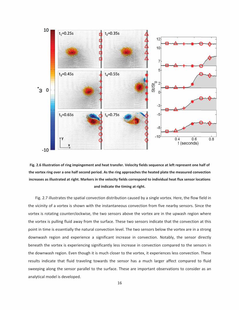
Fig. 2.6 Ill
the vortex
increases
Fig. 2
the vicinit
vortex is
the vortex
point in ti
downwas
beneath t
the down
results in
sweeping
analytical
lustration of ri
x ring over a on
as illustrated a
.7 illustrates t
ty of a vortex
rotating coun
x is pulling flu
ime is essenti
h region and
the vortex is
wash region.
dicate that f
along the se
model is dev
ing impingeme
ne half second
at right. Marke
the spatial co
x is shown wi
nterclockwise
uid away from
ially the natu
d experience
experiencing
Even though
fluid travelin
ensor parallel
veloped.
ent and heat tr
d period. As th
ers in the velo
and indicat
onvection dist
ith the instan
e, the two se
m the surface
ral convectio
e a significan
g significantly
h it is much c
g towards th
l to the surfa
16
ransfer. Veloci
e ring approac
ocity fields corr
te the timing a
tribution caus
ntaneous con
nsors above
e. These two
on level. The t
nt increase in
y less increase
loser to the v
he sensor ha
ace. These ar
ity fields seque
ches the heate
respond to ind
at right.
sed by a singl
vection from
the vortex ar
sensors indic
two sensors b
n convection
e in convectio
vortex, it expe
as a much la
e important
ence at left re
ed plate the m
dividual heat fl
le vortex. Her
m five nearby
re in the upw
cate that the
below the vor
n. Notably, th
on compared
eriences less
arger affect c
observations
present one h
easured conve
lux sensor loca
re, the flow fi
sensors. Sinc
wash region w
convection a
rtex are in a s
he sensor di
d to the sens
convection. T
compared to
s to consider
alf of
ection
ations
ield in
ce the
where
at this
strong
rectly
ors in
These
o fluid
as an

Fig. 2.7 Clo
the vortex
2.6 AMThe c
vortex is
hypothesi
surface c
through t
fluid struc
By definin
R.M.S flu
increases
2.6.1 A
ose up of inter
x experience m
Mechanist
urrent effort
based on the
ized that wh
auses an inc
he laminar bo
cture as a sem
ng the time s
uctuating vel
in the time a
A time resolv
raction proces
more convectio
com
tic Model
to develop a
e surface rene
en a flow str
crease (augm
oundary laye
mi infinite me
scale as the
locity, this m
averaged heat
ved model
s and measure
on than the se
mpared to sen
a physically b
ewal model o
ructure penet
mentation) in
r. This proces
edium. Heat is
hT
ratio of the
model succe
t transfer coe
17
ed rate of conv
ensor directly b
sors in the upw
ased model t
of Nix et al. (
trates throug
the rate of
ss was model
s conducted t
S
q kT T
mean stream
essfully predi
efficient (Nix,
vection. The se
beneath the vo
wash region.
to predict the
Nix, Diller et
gh the bound
heat transfe
ed as a purely
to the structu
k
m wise integr
icted experim
Diller et al. 2
ensors in the d
ortex and muc
e convective t
al. 2007). In
dary layer, int
er over that
y conductive
ure for a char
ral length sca
mentally me
2007).
downwash reg
ch more conve
transport due
their work, i
teraction wit
due to tran
event treatin
acteristic tim
ale to stream
easured valu
gion of
ection
e to a
it was
th the
nsport
ng the
e .
2.9
m wise
es of

Using
time depe
near a he
induces a
the bound
fluid temp
the boun
increase.
plate. On
the amou
governing
of the the
Fig. 2.8 Sc
convection
The chara
boundary
these valu
identified
g the surface
endent physi
eated surface
velocity field
dary layer. Th
perature (T )
dary layer, m
Thermal ene
ce the entrai
unt of therma
g the heat tra
ermal bounda
chematic used
n in the downw
acteristic tim
y layer to rea
ues are estim
location. Th
renewal mod
cs of the vor
e with a ther
d according to
his process ca
), move throu
mixing with t
rgy, therefor
ined fluid rea
l energy that
nsfer is the ti
ary layer to th
in model deve
wash region co
e is depende
ch the surfac
mated from th
e average ind
del described
rtex surface i
rmal boundar
o the Biot Sa
an be though
ugh the therm
the warmer
re, is being tr
aches the sur
has already
ime required
he heated sur
elopment alon
ompared to th
ent on two f
ce (d) and th
he velocity fie
duced velocit18
above, a sim
nteraction. C
ry layer of th
vart law (Pan
ht of as individ
mal boundary
near wall flu
ansferred to
rface, the res
been transfer
for the conve
rface.
ng with functio
he upwash regi
dBC.
factors: the d
he average in
eld produced
ty is approxim
mple model is
Consider the
hickness T as
nton 2005) w
dual fluid ele
y layer, and in
uid occurs an
the entraine
sulting condu
rred to it. Thu
ected fluid el
onal model res
ion due to the
distance that
nduced veloci
by a free vor
mated assumi
developed w
case of a sin
s shown in Fi
which forces o
ements which
nteract with t
nd causes th
d fluid prior t
uction is dimi
us, the charac
ements to tra
sults. Model pr
e shorter value
t the vortex
ity along this
rtex of specifi
ing a linear d
which capture
gle vortex lo
ig. 2.8. The v
outer fluid thr
h start at the
he surface. W
he temperatu
to its reachin
nished becau
cteristic time
avel from the
redicts much l
e of dBA compa
travels withi
s distance. Bo
ied strength a
drop to zero a
es the
cated
vortex
rough
outer
Within
ure to
ng the
use of
scale
e edge
arger
red to
n the
oth of
at the
at the

19
surface and is therefore one half the induced velocity at the edge of the boundary layer (point B)
calculated from the Biot Savart law. For point A, this is:
1 1 ( )( ) ( )2 2 2 ( )IND
OB
tV t V td t 2.10
The characteristic time for point A is then:
( )( )
BAd ttV t
2.11
While the model described above is very simple, the change in dBAallows it to capture the upwash
versus the downwash effect as shown in Fig. 2.7. This is illustrated in Fig. 2.8 by plotting the model
prediction as a function of non dimensional vortex location (y/L). Note that while points A and C are
equidistant from the vortex center, point A experiences much more convection because dBA<dBC. This
curve is similar in shape to the experimentally obtained curve shown in Fig. 2.7.
It is expected that a vortex will not have an immediate effect on the surface convection. Therefore,
it is necessary to incorporate a time delay to account for the time required for the induced outer fluid to
reach the surface. The appropriate time scale is the ratio of the thermal boundary layer thickness ( T)to
the average induced velocity (Eq. 2.10). Physically, this represents the shortest time that it would take
the outer fluid to cross the thermal boundary layer.
( )T
Delay tV t
2.12
Due to the square root in the denominator of the time averaged augmentation model (Eq. 2), the
instantaneous model has a factor of two in the denominator relative to the time average result in Eq. 2
from the integration. Incorporating the time delay and the factor of two, the heat transfer coefficient
augmentation prediction at point A becomes:
2Delay
kh t tt 2.13
Adding this augmentation to the heat transfer coefficient of the undisturbed boundary layer as the
square root of the sum of the squares gives:

20
220Delay Delayh t h h t 2.14
as the total magnitude as a function of time. This always results in an increase shifted in time for the
total heat transfer coefficient.
2.7 Comparison of the analytical model and experimental resultsThe analytical model was used to predict the transient convective heat transfer coefficient at the
heat flux sensor locations using the properties of the vortices identified in the TRDPIV measurements. In
all, 33 comparisons were performed. The following section along with Fig. 2.9 through Fig. 2.11 gives a
detailed description of the interaction process for the same sensor location for tests with vortex
Reynolds numbers of Re =3100, 5800, and 9200. For comparison, the tests labeled Re =5800 in the
following three figures examines the flow field and the convection at the fourth heat flux sensor from
the top for the test shown in Fig. 2.6. Fig. 2.12 then summarizes the results for all the tests.
The measured transient circulation and the induced velocity at a single sensor location are shown in
Fig. 2.9 for three vortex strengths spanning the range of test conditions. As the vortex ring propagates
towards the plate, the circulation remains nearly constant. Then, upon reaching the plate, vorticity of
opposite sign is generated at the wall and the vortex strength quickly diminishes. This is seen as the
abrupt drop in circulation at t=0.275s, t=0.655s, and t=1.39s for the three tests shown. The different
times are due to the smaller self induced propagation velocity for the weaker vortex rings (it takes
longer for them to propagate from the edge of the TRDPIV ROI to the plate). Incorporating these
measured vortex circulations with the measured vortex position, the transient induced velocity at a
sensor on the plate’s surface was calculated for each test using the Biot Savart law as shown in Fig. 4.b.
Since in each test the vortex follows approximately the same trajectory, the two main differences are
the speed at which the vortex passes the sensor and the induced velocity at the sensor, both of which
are affected by the circulation value. Consequently, the strongest vortex with the largest Re causes the
largest induced velocity for a short period of time while the weakest vortex causes a smaller induced
velocity for a longer period of time.

Fig. 2.9 Me
t
The c
the fluid t
Re =5800
2.10. Spe
expanded
larger for
sensor fro
Therefore
boundary
times the
the senso
possible v
layer, nor
dBA with
decreases
easured circul
to calculate th
haracteristic
travels within
test. Curves
cifically, the
d in time. The
r the weaker
om the top f
e, the Biot Sav
y layer at a sh
thermal bou
or transitions
value of T w
rmal to the su
the induced
s but then beg
ation of vortex
he induced velo
time used in
n the thermal
for the othe
curves for d
e characteris
vortices. It is
or this test. A
vart law pred
hallow angle
undary layer t
s to being in
which implies
urface. The c
velocity to
gins to increa
x as it approac
ocity at the se
the model is
boundary lay
er tests are n
BA are essent
tic time curv
s helpful to a
At the beginn
dicts that fluid
from beneat
thickness. As
n a downwa
s that the flu
haracteristic
produce the
ase at the end
21
ches the plate
nsor location o
s a function o
yer (dBA). Fig.
not shown du
tially identica
ve is smaller
again examine
ning of the te
d impacting t
th. Therefore,
the vortex m
sh region an
uid is essenti
time ( ) was
curve show
d as the induc
for three diffe
on the plate u
of the induced
2.10 shows d
ue to their si
al in magnitu
in magnitude
e Fig. 2.6 as
est, the vorte
he sensor wo
, the predicte
moves closer t
nd the distan
ally passing s
then calculat
wn in Fig. 2.1
ced velocity (
erent tests. Th
sing the Biot S
d velocity and
dBA as a funct
milarity to th
de and are o
e for the stro
dBA is calcula
ex is slightly
ould travel th
ed distance is
to and more
nce approach
straight thro
ted by combi
10. The time
and circulatio
e circulation is
Savart law
d the distance
tion of time fo
hose shown i
only contract
onger vortice
ated for the f
above the se
rough the the
s more than
above the se
hes the min
ugh the bou
ining the curv
decreases a
on) decrease.
s used
e that
or the
n Fig.
ted or
s and
fourth
ensor.
ermal
three
ensor,
imum
ndary
ve for
as dBA

22
Fig. 2.10 The distance that fluid must travel within the thermal boundary layer (dBA, +) is calculated from the
measured vortex location. Combing this value with the induced velocity from above yields the characteristic
time ( , ) used in the model. Re =5800
The characteristic time ( ) and the time delay ( Delay) were calculated for each sensor location for
each test. Plugging these values into Eqs. 2.13 and 2.14 yields a prediction of the convection as a
function of time at that point. Fig. 2.11 shows a comparison of the measured and predicted convection
at a single sensor location for three tests spanning the range of vortex strengths tested. The gap in the
prediction at t=0 for each test represents the initial calculated time delay, Delay. For all t<0, the vortex
has not yet entered the TRDPIV ROI and the prediction is therefore the natural convection (undisturbed)
Stanton number. At t=0, the vortex first enters the ROI, the model is applied and combined with the
natural convection Stanton number and delayed as specified. Then, as the vortex approaches the plate,
the induced velocity increases and dBA decreases causing a shorter and shorter characteristic time which
in turn causes the predicted convection to increase. Physically, the entrained fluid is spending less and
less time within the thermal boundary layer and is removing heat more effectively upon impact with the
surface. Comparing the transient model prediction with the measured convection, the two match well in
both shape and magnitude. Particularly, predictions at the point of highest augmentation are the most
accurate in terms of both magnitude and timing.

Fig. 2.11 C
Simila
condition
character
shown in
indicated
causes a
augmente
The m
pushing o
simplicity
Comparison of
t
ar results wer
s and 5 sens
ize the resu
Fig. 2.12. In o
by the dotte
smaller char
ed heat transf
model’s prom
outer fluid t
of the mod
model predict
three represen
re observed f
sor positions
lts, the maxi
over 80% of t
ed lines. As t
racteristic tim
fer coefficien
mising results
hrough the
el and the e
tion to measur
ntative tests sp
for all of the
. All of the
imum values
the cases the
the vortex st
me and small
nt predicted b
clearly demo
boundary la
ase in which23
red convection
panning the ra
33 vortex rin
heat flux cur
s of the mea
e model predi
trength incre
er time dela
by equation 6
onstrate that
yer which th
h it can be im
n during vortex
ange of vortex
ng tests exam
rves were sim
asured and m
icts the meas
eases, the ind
y in the mod
.
coherent str
hen conducts
mplemented
x interaction.
strengths.
mined spanni
milar to thos
modeled Stan
sured convect
duced velocit
del. This dire
uctures incre
s heat from
make the re
Results shown
ng 5 differen
se in Fig. 2.1
nton number
tion within 15
ty increases w
ectly increase
ease convecti
the surface
sults all the
n from
nt test
11. To
rs are
5% as
which
es the
on by
e. The
more

encourag
fundamen
current ef
Fig. 2.12
2.8 CoIn this
a surface
measurem
it is a fund
the conve
structure
mechanis
times for
through t
Converse
has alread
heat flux
surface lo
ing. The ultim
ntal understa
fforts are ong
Comparison o
onclusions
s investigatio
e was studied
ments. This in
damental pro
ection from th
and the surf
tic model wa
the fluid mo
the boundary
ly, regions wh
dy been hea
was calculate
ocations for a
mate applica
anding of the
going.
of the maximum
test conditio
s
n, the convec
d experimen
nteraction had
oblem of both
his coherent s
face. Based o
as developed
otion through
y layer, the
here fluid is s
ted within th
ed using this
range of vor
ation is to m
effects of tu
mmeasured c
ons. The dotted
ctive heat tra
tally using s
d not been p
h convective f
structure inte
on an analys
using the pa
h the bounda
convection i
swept along t
he boundary
simple mode
rtex speeds a
24
model vortice
rbulence on
convection wit
d lines represe
ansfer resultin
patiotempor
reviously stud
fluid mechan
eraction is du
is of the tim
arameters of
ary layer. In
is high beca
the surface e
layer prior t
el and compa
nd strengths
s in turbulen
surface trans
h maximumm
ent the + 15%
ng from the i
ally resolved
died in detail
ics and turbu
ue to transien
me dependent
f the vortices
regions whe
use the fluid
experience les
to reaching t
red to the m
. For the par
nce which w
sport. It is in
model predictio
bounds.
nteraction of
d flow and s
which is surp
ulence. The re
t heat condu
t flow and su
s to calculate
ere vortices f
d quickly rea
ss convection
he surface.
easured conv
rameter space
ould increas
this direction
on for the rang
f a ring vortex
urface conve
prising consid
esults indicate
ction betwee
urface heat f
the characte
force fluid di
aches the su
n because the
The time res
vection at mu
e investigated
e our
n that
ge of
x with
ection
dering
e that
en the
flux, a
eristic
rectly
rface.
e fluid
solved
ultiple
d, the

25
model was very accurate at predicting the time resolved convection resulting from the coherent
structure interaction. This transport mechanism has important implications for understanding the role
of coherent structures in turbulent flows.
26
3 A Mechanistic Model of Turbulent Heat Transfer Augmentation in
Stagnation Flow
David O. Hubble, Pavlos P. Vlachos, and Tom E. Diller
3.1 AbstractA time resolved experimental study has been performed examining the mechanism by which heat
transfer is augmented in stagnating flows by freestream turbulence. Recent work has demonstrated that
turbulence is amplified into strong vortices in the stagnation region which then dominate the near wall
flow. By utilizing time resolved digital particle image velocimetry (TRDPIV) and a new variety of heat flux
sensor called the time resolved heat and temperature array (THeTA), the spatio temporal influence of
these structures on the heat transfer is examined. The current study confirms that coherent structures
are the primary mechanism for the observed heat transfer augmentation in stagnating flows. It is shown
that large increases in convection occur in regions where the structures force freestream fluid through
the thermal boundary layer to the surface. Evidence supporting this mechanism is provided by the
success of a simple mechanistic model which was recently developed by the authors. The model is able
to accurately predict the time resolved convection at any point on the surface based solely on the
transient properties of the large scale structures present.
3.2 Nomenclaturea = acceleration parameter (1/s)
= thermal diffusivity (m2/s)
b = grid bar diameter (cm)
= thermal expansion coefficient (1/K)
C = specific heat (J/kg K)
d = distance (m)
= boundary layer thickness (m)
= circulation (m2/s)
h = convective heat transfer coefficient (W/m2 K)
k = thermal conductivity (W/m K)
L = stagnation body height (cm)
= turbulence integral length scale (cm)
= kinematic viscosity (m2/s)
27
Pr = Prandtl number
q” = heat flux (W/m2)
= density (kg/m3)
St = Stanton Number
t = time (s)
T = temperature (K)
= time delay (s)
Tu = turbulence intensity (%)
U = velocity (m/s)
Subscripts
0 = laminar baseline level
= freestream
S = surface
T = thermal boundary layer
3.3 IntroductionFreestream turbulence has a major effect on surface heat transfer in many engineering applications,
for example, gas turbines, combustors, electronic cooling devices, and heat exchangers. Modeling the
surface heat transfer under such circumstances is difficult even for simple flows and geometries because
of the unpredictable effect of the freestream turbulence. Traditionally, methods for analyzing the
convective heat transfer when freestream turbulence exists rely on average and statistical properties of
the flow field. The analysis results in empirical correlations which lack a physical foundation and ignore
the time dependent processes. Therefore, it comes as no surprise that no single correlation can capture
all available experimental data. In order to understand and model the mechanism by which these
processes occur it is necessary to study the detailed transient properties of the flow field in conjunction
with the time resolved heat transfer during the interaction.
In order to understand the effect of freestream turbulence on surface transport, it is important to
characterize the coherent structures present and determine how they interact with the surface
boundary layer. In a recent paper, large scale coherent structures were shown to play a dominant role in
turbulent flows (Adrian 2007). Experiments have also shown the existence of very large scale motions in
the logarithmic region of turbulent boundary layers which can reach up to 20 times the boundary layer

28
thickness in size (Hutchins and Marusic 2007). These coherent structures have been identified to be
important contributors to transport in boundary layers. This is particularly true in stagnation regions
where structures are amplified into strong vortices at the surface by the mean flow strain rate (Sutera
1965; Blackwelder 1988; Wei and Miau 1992). Heat and mass transport at the wall appear to be directly
affected by the sweeping of these large vortices into the boundary layer, particularly at higher levels of
turbulence intensity (Thole and Bogard 1995; Mosyak, Pogrebnyak et al. 2001). VanFossen and
Simoneau (Vanfossen and Simoneau 1987) used wires to create large vortices perpendicular to a
downstream cylinder and studied the resulting fluid flow and heat transfer near the surface using a
combination of smoke visualization and liquid crystals. Regions where vortices forced fluid toward the
surface (downwash) corresponded to regions of increased heat transfer. Measurements of the
fluctuating transport at the surface have shown direct correlation with the velocity fluctuations in the
freestream (Simmons, Hager et al. 1990; Moss and Oldfield 1996; Holmberg and Diller 2005) but the
impact on the overall transport was not established.
Marusic et al. (Marusic, Mathis et al. 2010) recently developed a model based on fluid experiments
which predicted the near wall turbulence given only large scale information from the outer boundary
layer region. The success of their model showed that the small scale structure was directly influenced by
the large scale outer structures. In a similar fashion, the authors (chapter 2 of this dissertation)
developed a time resolved model to predict the convection resulting from the interaction of a single
vortex with a surface. The model was tested experimentally by comparing its prediction to the measured
convection during the collision of a vortex ring with a wall. Results indicated that the model performed
quite well. In the following section the model is briefly described.
In the current work, heat transfer augmentation in a stagnating turbulent flow is examined
experimentally. During the test, the spatiotemporally resolved convective heat transfer coefficient along
the stagnation line is examined in conjunction with the fully resolved two dimensional flow field.
Combining these measurements gives a quantitative picture of the transport mechanism and provides
valuable insight into the physics of the interaction. Finally, the previously developed mechanistic model
is applied to the current data and used to predict the transient convection from a more realistic flow
field which contains multiple simultaneous vortices.
3.4 Mechanistic Model

29
A simple model of the mechanism of heat transfer augmentation by a coherent structure was
recently developed based on experimental observations of a vortex ring collision with an instrumented
heated plate. The model predicts the time resolved increase in convection over laminar levels based
only on the properties of the vortex present. Heat transfer to the structure is modeled as a purely
conductive event treating the structure as a semi infinite medium. The resulting convection is then a
function of only a characteristic time scale for the interaction and the properties of the fluid.
S
q khT T t
3.1
Here, the characteristic time (t) can be thought of as a measure of how long a packet of fluid warms
prior to reaching the surface. The more heat that is transferred to the fluid before reaching the surface,
the less heat the fluid will be able to remove from the surface upon impact. By using the physical
properties of the nearby vortex to calculate the characteristic time, the model was able to accurately
predict the convection resulting from a vortex wall interaction. The following paragraphs briefly
describe the model inputs and how it is used to produce an overall convection estimate.
Fig. 3.1 is used to describe how the characteristic time can be calculated from vortex properties. A
vortex is located at point O a distance L from a heated surface where a thermal boundary layer of
thickness T exists. The characteristic time is defined as the time required for freestream fluid to pass
from the edge of the thermal boundary layer to the surface. To determine this time, both a distance and
an average velocity are needed. By the Biot Savart law, the vortex induces a velocity at a surface point A
that is a function of the vortex circulation, , and the distance from the vortex to the surface, dOA. Since
the Biot Savart law also gives the trajectory of the fluid, it can be used to determine where, for a given
surface location, the fluid crossed into the thermal boundary layer. The distance that fluid traveled
within the boundary layer can then be determined from this information (dBA for example). Assuming
the velocity decreases linearly from the Biot Savart prediction at B to zero at A, the characteristic time
becomes:
41
2
OA BABA
IND
d ddtV 3.2
Note that the model automatically accounts for the difference between the upwash and downwash
region of a vortex. While both A and C are equidistant from the vortex, A predicts higher augmentation
(smaller t) because dBA is much shorter than dBC.

To co
convectio
experime
Finally, th
of the sum
heat trans
Fig. 3.1 Sc
in th
In the
the collis
complicat
multiple v
3.5 ExThe e
of a bluff
Image Ve
resolved
(Hubble a
omplete the
on. The time s
nt was the ra
he predicted
m of the squa
sfer coefficien
chematic used
he downwash r
e original pap
ion of a vort
ted flow field
vortices of dif
xperimenta
xperiments fo
body in a flow
elocimetry (T
velocity mea
and Diller 201
model it mu
scale that wa
atio of the th
augmentatio
ares to produ
nt when no fr
d in model dev
region due to
per, the mode
tex ring with
of a stagnat
fferent sizes a
al Method
or the data re
w which cont
TRDPIV) (Raff
asurements w
10) was used t
ust be prope
s chosen for
ermal bound
n (Eq. 3.1) is
uce a total co
reestream tu
velopment with
the shorter dis
el was succes
h a heated s
ing turbulent
and strengths
dology
eported in th
tains large sca
fel, Willert e
while the new
to measure t
30
erly delayed
the time dela
ary layer thic
combined w
nvection pred
rbulence is pr
h functional m
stance that flu
sfully used to
urface. In th
t flow. Here, t
s which exist t
is work exam
ale freestream
et al. 2007)
w Time Reso
he convectio
and combin
ay and which
ckness to the
with the basel
diction. In thi
resent.
model results. M
uid travels with
o predict the
he current w
the convectio
together.
mine the conve
m turbulence
was used to
lved Heat an
n from the he
ned with the
h worked wel
e ½ VIND value
ine level usin
is case, the b
Model predicts
hin thermal bo
time resolve
ork, it is app
on is strongly
ection along t
e. Time Resolv
o provide fu
nd Temperatu
eated stagnat
e laminar bas
l in the vorte
e calculated a
ng the square
aseline level
s larger conve
oundary layer.
d convection
plied to the
y influenced b
the stagnatio
ved Digital Pa
ll flow field,
ure Array (TH
tion model. A
seline
x ring
bove.
e root
is the
ction
from
more
by the
on line
article
time
HeTA)
All the

tests wer
grids wer
were use
performe
present. A
in Fig. 3.2
3.5.1 W
The w
operated
construct
is approxi
Fig
Freest
was base
construct
constant t
the meas
geometry
e performed
re used to co
ed producing
d, two each
A schematic d
.
Water Tunne
water tunnel
at 10cm/s f
ed from clea
imately 1% th
. 3.2 Water tu
tream turbul
ed on correla
ed with solid
turbulence in
ured flow fie
y and turbulen
in a water t
ontrol the fre
g 3 different
at each turb
depicting the
el Facility an
used in the c
for all tests.
r acrylic. At t
hroughout the
nnel facility an
ence was gen
ations by Ba
dity ratios of 0
ntensity of 7.1
ld using the m
nce propertie
Table 3
tunnel at a co
eestream turb
t freestream
bulence cond
relative posi
nd Turbulen
current exper
The test se
he tunnel spe
e test section
nd position of
nerated using
ines and Pe
0.7 to give in
1%. The prop
method desc
es are given in
3.1 Details of g
31
onstant frees
bulence char
m turbulence
dition includi
tions of the e
nce Generat
riment is a clo
ection measu
eed used in t
n.
model relative
g simple bi pla
terson (Bain
ntegral length
perties of the
ribed by Giffo
n Table 3.1.
grids and turb
stream veloc
racteristics at
conditions.
ng a low tur
equipment us
ion
osed loop, va
ured 0.61m
he test, the f
e to turbulenc
ane grids. Gr
es and Pete
h scales of ap
generated tu
ord (Gifford,
ulence statisti
ity of 10cm/s
t the test loc
A total of
rbulence base
sed in the exp
ariable speed
square by 1
freestream tu
ce grid and TRD
id bar sizing (
rson 1951).
pproximately
urbulence we
Diller et al.).
ics
s. Passive bi
cation. Three
eight tests
eline with no
periment is s
facility which
1.77m long a
urbulence inte
DPIV system.
(b) and positi
Three grids
1, 2, and 3cm
re calculated
Details of th
plane
grids
were
o grid
hown
h was
and is
ensity
oning
were
m at a
from
e grid
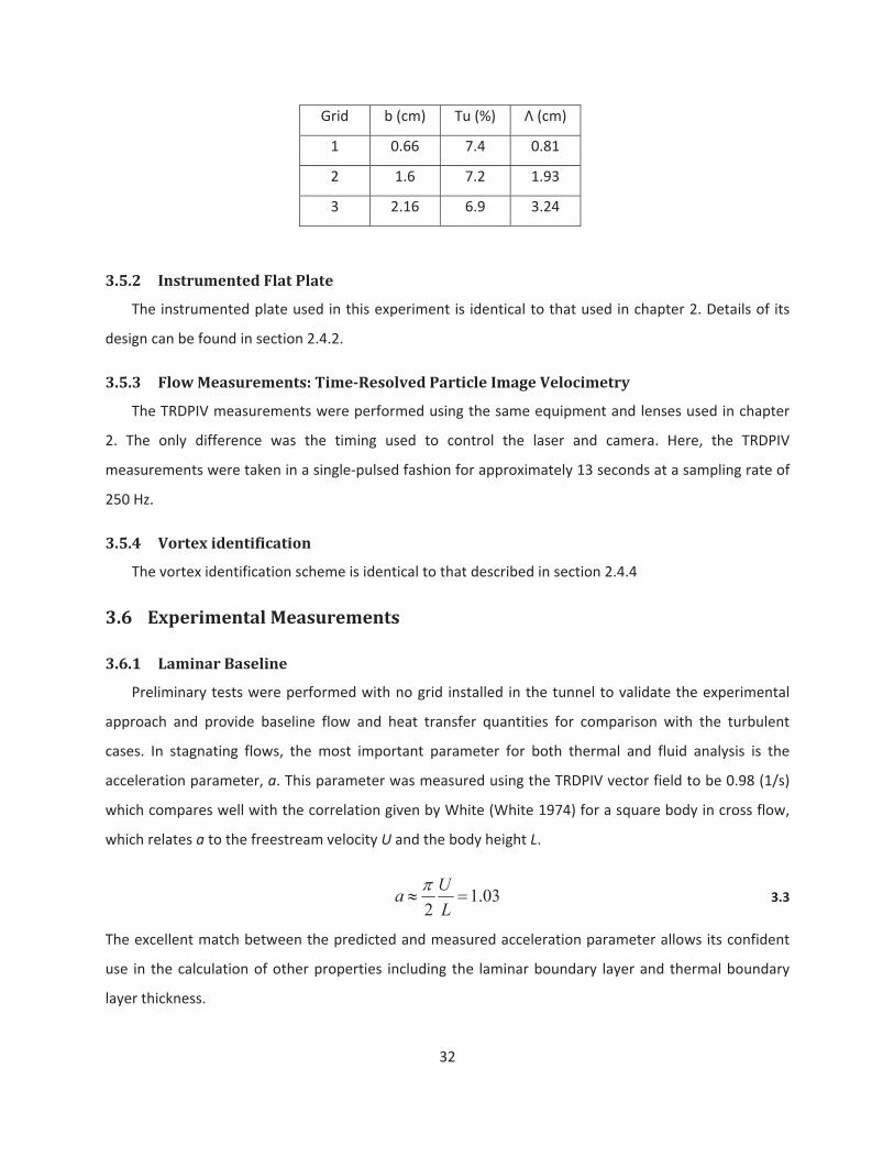
32
Grid b (cm) Tu (%) (cm)
1 0.66 7.4 0.81
2 1.6 7.2 1.93
3 2.16 6.9 3.24
3.5.2 Instrumented Flat Plate
The instrumented plate used in this experiment is identical to that used in chapter 2. Details of its
design can be found in section 2.4.2.
3.5.3 Flow Measurements: Time Resolved Particle Image Velocimetry
The TRDPIV measurements were performed using the same equipment and lenses used in chapter
2. The only difference was the timing used to control the laser and camera. Here, the TRDPIV
measurements were taken in a single pulsed fashion for approximately 13 seconds at a sampling rate of
250 Hz.
3.5.4 Vortex identification
The vortex identification scheme is identical to that described in section 2.4.4
3.6 Experimental Measurements
3.6.1 Laminar Baseline
Preliminary tests were performed with no grid installed in the tunnel to validate the experimental
approach and provide baseline flow and heat transfer quantities for comparison with the turbulent
cases. In stagnating flows, the most important parameter for both thermal and fluid analysis is the
acceleration parameter, a. This parameter was measured using the TRDPIV vector field to be 0.98 (1/s)
which compares well with the correlation given by White (White 1974) for a square body in cross flow,
which relates a to the freestream velocity U and the body height L.
1.032
UaL
3.3
The excellent match between the predicted and measured acceleration parameter allows its confident
use in the calculation of other properties including the laminar boundary layer and thermal boundary
layer thickness.

33
0.42.4 PrTa3.4
Using the kinematic viscosity ( ) and Prandtl number (Pr) at the film temperature gives =0.21 cm and
T=0.11cm. The acceleration parameter can also be used to predict the baseline heat transfer coefficient
from the surface using the correlation given by Goldstein (Goldstein 1938).
0.420 0.5421 Pr ah k 3.5
Equation 3.5 predicts a baseline heat transfer coefficient of h0=731 W/(m2K) which matches the value of
h0=755 W/(m2K) measured by the THeTA to within the experimentally uncertainty. The measured
convective heat transfer coefficients are made into the dimensionless Stanton number by dividing by
the product of the freestream velocity, specific heat, and density (U C ).
h tSt t
CU3.6
3.6.2 Transient Flow and Convection: Physical Insight of the Mechanism
As turbulence enters the stagnation region, it is stretched and amplified into vortices which interact
with the near wall fluid and cause large increases in the instantaneous convection. This interaction is
illustrated in Fig. 3.3 in which the instantaneous flow field and simultaneous convection are shown. By
utilizing the multiple sensing locations of the THeTA, the mechanism by which the vortices increase the
convection is easily shown. At left, a segment of the TRDPIV ROI is shown which contains multiple
vortices interacting with five THeTA sensing location as indicated by the black dots. The contour of the
vector plot indicates the U velocity magnitude and helps to illustrate where fluid is moving towards and
away from the surface. At right, the bar plot represents the instantaneous convection at the five sensing
locations shown relative to the laminar baseline.

Fig. 3.3 I
dots and
m
In the
rotation o
expected,
freestream
upwash c
pulled alo
fluid while
An alt
shown alo
identified
indicates
identified
sensors a
surface a
towards t
the down
approach
close to t
Instantaneous
d convection m
magnitude of t
e TRDPIV me
orientation w
, the downw
m is being fo
orrespond to
ong the heate
e traversing t
ternative way
ong with the
vortex (with
the measure
as indicated
s indicated b
nd has little
the surface an
wash region
es the surface
he surface, it
s snap shot of t
measurements
the U velocity.
asured vecto
which produc
wash regions
orced into th
o low levels o
ed surface pri
the surface, it
y to view the
e convection
h clockwise ro
d circulation
by the color
y the marker
impact of th
nd its circulat
and experien
e, the convec
ts image in th
the flow field a
s are given by
. Convection in
or field, there
ces alternatin
correspond
e thermal bo
of convection
or to reachin
t is ineffective
interaction is
time historie
otation) is sh
of the vortex
bar at right.
rs in the left f
he convectio
tion is amplif
nces more tha
ction from the
he wall (pote
34
and convectio
the bars at rig
ncreases are lo
e are three s
ng areas of d
to high leve
oundary layer
since the flu
g these locat
e at removing
s shown in Fig
es at three s
own over a t
x while its co
The measure
figure. At firs
on over the f
fied. At this p
an double the
e middle sens
ential flow the
on. Sensor loca
ght. The contou
ocalized to are
trong vortice
downwash a
ls of convec
r in these re
uid at the sur
ions. Since he
g heat in thes
g. 3.4. Here, a
sensors locat
time period o
olor correspon
ed convection
st, the vortex
first two seco
oint, the top
e laminar bas
sor also incre
eory) causes
ations are indic
ur of the vecto
eas of vortex d
es at the surf
nd upwash a
tion since co
gions. Altern
rface in these
eat has been
e upwash reg
a single trans
ted in the vic
of 5.3 s. the s
nds to the tim
n is shown at
x is both weak
onds. Then,
sensor is pos
seline convect
ases slightly.
it to move d
cated by the b
or field shows
ownwash.
face of altern
at the surfac
ool fluid from
atively, regio
e regions has
transferred t
gions.
ient vortex tr
cinity. At left
size of the m
me at which i
right for the
k and far from
the vortex m
sitioned direc
tion. As the v
Once the vor
ownward bri
lack
the
nating
ce. As
m the
ons of
been
to this
rack is
t, the
marker
it was
three
m the
moves
ctly in
vortex
rtex is
inging

the middl
a true do
middle se
as the vo
baseline l
remained
Fig. 3.4 T
strength a
3.7 CoThe a
coefficien
measurem
to preven
were ma
measurem
the meas
interactio
Fig. 3
of test #1
correspon
e sensor into
ownwash reg
ensor does ex
ortex continue
level. Since t
below the ba
Transient inter
re indicated b
omparison
analytical mo
nt at the heat
ments. For ea
nt vortices fr
de (3 grids
ments. The fo
sured convec
ons from one
.5 shows the
1 of grid 2. As
nds to the tim
o a downwash
ion the vorte
xperience an i
es to move f
the bottom s
aseline level f
raction of a sin
y the circular m
history
n of the ana
odel was tes
t flux sensor l
ach of the tur
om outside t
X 2 trials
ollowing secti
ction and th
of the tests. T
three vortex
s in Fig. 3.4, t
me. At right
h region. Not
ex has move
increase in co
from the surf
sensor remain
for nearly the
ngle vortex wit
markers at left
y for three nea
alytical m
sted by using
ocations usin
rbulent cases
the TRDPIV R
X 6 sensors
on along wit
he fluid stru
Table 3.2 the
x tracks that in
he marker’s s
is the norma
35
e, however, t
d farther fro
onvection but
face and lose
ned in the u
e entire test.
th the surface
t while the col
arby sensor loc
odel and e
g it to pred
ng the proper
s, comparison
ROI from infl
s) for the en
h Fig. 3.5 thr
ucture during
n summarize
nfluence one
size indicates
alized Stanton
that by the ti
om the surfac
t not to the e
e strength, th
pwash region
and resulting
lor correspond
cations is show
experimen
ict the trans
rties of the vo
ns were made
uencing the
ntire 13 sec
ough Fig. 3.8
g a particula
s the findings
particular se
s the circulati
n number me
me that the m
ce and weak
xtent of the t
he convection
n of the vort
convection. Vo
ds to the time
wn.
ntal result
sient convect
ortices identi
e for the cent
results. In al
cond duratio
8 gives a deta
arly interesti
s from the rem
ensor over the
on of the vor
easured by th
middle senso
kened slightly
top sensor. Fi
n falls back t
tex, its conve
ortex location
at right. Conve
ts
tive heat tra
fied in the TR
ter 6 sensors
ll, 36 compar
on of the TR
ailed descripti
ing set of v
maining tests
e final 3.5 sec
rtex while its
he sensor an
or is in
y. The
inally,
to the
ection
and
ection
ansfer
RDPIV
s (3 8)
risons
RDPIV
ion of
vortex
s.
conds
color
nd the

vertical d
shown be
the senso
Fig. 3
(circula
Exam
the meas
delineate
sensor (+)
strong vo
the vorte
boundary
strength
measured
starts app
compared
layer tow
vortex be
3 appears
otted lines d
ecause it caus
or location at t
3.5 Three vorte
ation) of vortex
ining Fig. 3.5
sured vortex
s between th
) and the me
rtex in the vic
x which mos
y layer thickn
as it approa
d convection.
proximately t
d to 3.5cm2/s
wards the sen
gins to move
s and quickly
delineate bet
sed the smalle
that point in
ex tracks and r
x while the fill
along with Fi
properties o
he three trac
easured circu
cinity of the s
st strongly in
esses away a
ches the sta
Then, at t=1
the same dis
. This clockw
sor, increasin
away and we
y grows into
tween the th
est calculated
time.
resulting meas
color correspo
conve
ig. 3.6 gives a
over the sam
ks. Specifical
lation ( ) is s
sensor and th
nfluences the
and has a cir
agnation regi
10.25s, a mor
stance from
ise rotating v
ng the conve
eaken, the co
a dominant36
hree tracks. T
d characterist
sured convecti
onds to the tim
ection is shown
a clearer pictu
me 3.5 secon
ly, the non d
shown. At th
he convection
convection
rculation of le
on (and the
re dominant
the sensor,
vortex forces
ction to almo
onvection ret
vortex. The
The vortex sh
tic time (large
on. Marker siz
me as indicate
n.
ure of the inte
ds as Fig. 3.
imensional d
he beginning
n is at nearly
at the senso
ess than 1cm
sensor) with
vortex emerg
it is stronge
fluid straight
ost 60% abov
urns to the b
counter cloc
hown at eac
est estimated
ze indicates re
d at right whe
eraction proc
.5 and again
distance from
of the time s
the baseline
or location is
m2/s. This vor
h a correspo
ges. Although
r with a circ
through the
ve baseline le
aseline level.
ckwise vortex
h point in ti
d augmentatio
lative strength
ere the measur
cess. Fig. 3.6 s
the vertical
m the vortex t
shown, there
level. At this
approximate
rtex then gro
onding increa
h vortex num
culation of 5
thermal bou
evels. Then, a
At t=11.7s, v
x forms abov
me is
on) at
h
red
shows
lines
to the
is no
time,
ely 13
ows in
ase in
mber 2
cm2/s
ndary
as the
vortex
ve the

sensor th
sensor, it
nearly 75%
enter the
vortex is s
From
3.7. The B
fluid must
the therm
traveling
surface pr
is proport
vortex. At
therefore
fluid prior
measured
third vort
its life, th
en moves do
s circulation
% higher than
e upwash reg
still quite clos
Fig. 3.
the measure
Biot Savart ca
t travel withi
mal boundary
nearly perpe
rior to reachi
tional to the
t t=10.6s, th
, is quickly tr
r to reaching
d convection.
ex. In this thi
he vortex is a
ownward alon
grows to a m
n the baselin
ion of the vo
se to the sens
6 Transient pr
ed vortex pro
alculated indu
in thermal bo
layer (values
ndicular to th
ng the senso
induced velo
e induced ve
raveling a sho
the surface.
Then, as the
rd vortex trac
bove the sen
ng the surfac
maximum of
e just as the
ortex, a drast
sor.
roperties of th
operties, the t
uced velocity
oundary layer
of dBA near o
he surface. La
r location. Th
ocity which i
elocity is at a
ort distance t
Note that in
e vortex dies
ck, the affect
nsor and, sinc
37
ce. As the vo
9cm2/s. This
vortex reach
tic decrease
e three vortice
transient mo
is shown ( )
r (dBA , +). Wh
one) the senso
arger values i
he average sp
s a measure
a local maxim
to reach the
Fig. 3.5, t=10
s, VIND falls to
t of upwash v
ce the vortex
ortex approac
s causes the
es the sensor
in convection
es during the i
odel inputs w
with the non
hen the fluid
or is in the do
indicate that
eed that the
of both the
mum and dBA
surface and
0.6s correspo
o essentially z
ersus downw
has counter
ches and eve
convection t
r. Then, as th
n is observed
nteraction tim
ere calculate
n dimensiona
travels a sho
ownwash reg
the fluid is sw
fluid travels a
strength and
A is at a loca
little heat is
onds to a loca
zero prior to
wash is most v
clockwise ro
ntually passe
o spike at a
e sensor beg
d even thoug
me
ed as shown i
l distance tha
ort distance w
ion and the f
weeping alon
along this dis
d proximity o
al minimum.
transferred t
al maximum i
the arrival o
visible. For m
otation, the s
es the
value
gins to
gh the
in Fig.
at the
within
luid is
ng the
tance
of the
Fluid,
to the
in the
of the
ost of
ensor

remains i
region. O
upwards a
has ample
In Fig
indicates
delineate
convectio
convectio
the therm
through t
distance
developed
of these la
convectio
the succe
time, one
n its downw
nce this occu
along the sur
e time to war
g. 3.8, the fin
the 3.5 seco
between th
on well in te
on both corre
mal boundary
the thermal
within the
d performs q
arge scale co
on can be mo
ess of the mo
e vortex is gen
ash. Once th
urs, fluid ente
rface prior to
rm as it slides
Fig. 3.7 Trans
al model pre
onds discusse
he different
erms of both
spond to tim
y layer. Time
boundary lay
thermal bou
uite well con
herent struct
odeled withou
odel also imp
nerally domin
he vortex pas
ers the therm
reaching the
along the su
sient model in
ediction is sh
ed in the pre
tracks. The
h shape and
mes when free
es of low con
yer (weak an
undary layer
nsidering the
tures can be a
ut solving for
plies that, alt
nant at a part
38
sses the sens
mal boundary
e sensor as in
rface and the
puts derived f
own with the
evious three
e transient m
magnitude.
estream fluid
nvection occu
nd/or distant
(upwash re
complexity o
accurately pr
r the fine sca
hough there
ticular locatio
or however,
layer far bel
ndicated by th
e heat transfe
from vortex pr
e measured c
figures and
model predi
The two dis
is quickly rea
ur either whe
vortex) or w
egion of vor
of the flow fie
edicted, using
ale motions i
are multiple
on. The added
the sensor e
ow the senso
he large value
er is reduced.
roperties
convection. T
the vertical d
ction match
stinct spikes
aching the se
en fluid is pa
when fluid m
rtex). The m
eld. Therefore
g LES for insta
n the near w
e vortices pre
d complicatio
enters the up
or and must t
e for dBA. This
The shaded r
dotted lines
es the mea
in the mea
ensor from ou
assing very s
must travel a
mechanistic m
e, if the form
ance, the res
wall region. Fi
esent at any
n of attempt
pwash
travel
s fluid
region
again
sured
sured
utside
slowly
great
model
mation
ulting
inally,
given
ing to

account f
vortex can
Fig. 3.8 M
Finally
it would
augmenta
laminar b
with incre
the smal
augmenta
interactio
for the affect
n be determin
Model predictio
y, since the m
be expected
ation. The res
baseline value
easing length
ler two leng
ation observe
ons.
Table
Grid
1
2
3
ts of multiple
ned.
on with measu
i
model works w
d to provide
sults are sho
e of h0=755W
scale. The m
gth scales. T
ed in the pas
e 3.2 Summary
(cm)
0.81
1.93
3.24
e different vo
ured convectio
in detail in the
well in predic
e an accurat
wn in Table
W/m2K. As in p
model accurat
This is a str
st is simply th
y of time avera
Meas
h (W/m2K)
1042
977
971
39
ortices at the
n. The shaded
e previous thre
cting the conv
te estimate
3.2 where th
previous stud
tely predicts
rong indicati
he overall ef
aged augment
sured
Aug (%)
38
29
29
surface can
region corres
ee figures.
vection during
of the time
he augmentat
dies, the mea
this trend wi
on that the
ffect of a num
tation and mod
Mo
h (W/m2K
1036
984
862
be eliminate
ponds to the 3
g individual v
averaged tu
tion is calcula
sured augme
ith particular
time averag
mber of thes
del predictions
odel
K) Aug (%)
37
30
14
ed if the dom
3.5 seconds stu
vortex interac
urbulent heat
ated based o
entation decr
ly good resul
ged heat tra
se transient v
s
minant
udied
ctions,
t flux
on the
reases
lts for
ansfer
vortex
40
3.8 ConclusionsThis work has successfully applied a simple vortex model to predict the increase in convection
observed in the stagnation region of a flow containing large scale freestream turbulence. It is shown
that coherent structures which form due to the amplification of vorticity dominate the flow field and
directly increase the convection. A simple model was developed to predict the resulting time resolved
convection based on the measured vortex location and circulation. Using the model, the resulting
convection was accurately predicted in a time resolved fashion taking only the transient properties of
the vortices present as inputs. Evidence supporting the model’s capabilities is provided by its successful
validation in turbulent flows of varying integral length scale. These promising results support the
hypothesis that coherent structures are the mechanism by which heat transfer is augmented in
turbulent flows. Modeling the affect of these structures gives a new approach to calculating the heat
transfer augmentation in turbulent flows once the large scale structure of the flow is known.
3.9 AcknowledgementsThe principle author would like to thank Dr. Andrew Gifford for his work developing and
characterizing the turbulence grids and stagnation model. This material is based upon work supported
by the National Science Foundation under Grant No. CTS 0423013. Any opinions, findings, and
conclusions or recommendations expressed in this material are those of the authors and do not
necessarily reflect the views of the National Science Foundation.

41
4 Development and Evaluation of the Time Resolved Heat and
Temperature Array
David O. Hubble and Tom E. Diller
Published in the ASME Journal of Thermal Science and Engineering Application, Vol. 2, Sept 2010
4.1 AbstractThe development and evaluation of a differential style heat flux gauge is presented. The sensor is
constructed from spot welded foils of copper and constantan on either side of a thin Kapton polyimide
film and is capable of measuring the heat flux and surface temperature at ten locations simultaneously.
Analytical modeling was performed to estimate the sensor’s sensitivity and time response. Calibrations
were performed in conduction and radiation yielding an average heat flux sensitivity of 20.4
V/(kW/m2). Time response measurements were also performed which gave an average 63% time
response of 168 milliseconds. The capabilities of the sensor are demonstrated by showing its use in
ongoing convection research.
4.2 Nomenclaturea = stagnation flow parameter (1/s)
= thermal diffusivity (m2/s)
C = specific heat (J/kg-K)
= sensor thickness ( m)
h = convective heat transfer coefficient (W/m2-oC)
k = thermal conductivity (W/m-oC)
L = characteristic length (m)
= kinematic viscosity (m2/s)
Pr = Prandtl number
= density (kg/m3)
q" = heat flux (W/m2)
R" = thermal resistance (oC/(W/m2))
S = sensitivity ( V/(kW/m2))
Se = Seebeck coefficient ( V/oC)
T = temperature (oC)
42
Tu = turbulence intensity (%)
T = time (s)
= time constant (s)
T = temperature difference (oC)
U = uncertainty
U = freestream velocity (m/s)
V = Voltage (volts)
V = voltage difference (volts)
Subscripts
0 = initial
1 = top
2 = bottom
G = glue
in = input
K = Kapton
out = output
P = paint
ref = reference
SS = steady state
TC = thermocouple
4.3 IntroductionThe accurate characterization of a thermal system requires the measurement of both temperatures
and energy fluxes. While temperatures can be measured in a variety of ways, the accurate measurement
of heat flux is still a challenge. This paper reports on the development and evaluation of a simple heat
flux sensor capable of acquiring multiple simultaneous, time resolved heat flux and surface temperature
measurements. This capability allows the sensor to measure the distribution of heat flux over a surface
to better describe the thermal environment. Examples of research areas where this sensor could be
used include gas turbines, electronics cooling, and biological systems.
Heat transfer rates have been measured using a variety of sensors operating on different principles
(Diller 1993). One popular type of heat flux sensor is the differential sensor. By measuring the

43
temperature drop across a known thermal resistance, the heat flux through the sensor is determined
using Fourier’s Law which, for 1 D steady state, reduces to
" kq T 4.1
assuming the properties of the thermal resistance layer are uniform and constant. In Eq. 4.1, k and are
the thermal conductivity and thickness of the resistance layer between the two temperature
measurements. The temperature difference across the thermal resistance layer ( T) can be measured
using either thermocouples or resistance temperature detectors (RTDs).
Thin film heat flux gages have certain advantages over other types of differential heat flux sensors.
It is generally possible to place a number of sensors on a single film which allows the heat flux to a
surface to be mapped. This is particularly important when investigating the effects of non uniform
boundary conditions on heat transfer, such as turbulence, jets, and transition. Another advantage is that
thin film gages can be made flexible, allowing them to be mounted to curved surfaces such as airfoils.
Thin sensors have a frequency response that is faster than traditional designs such as the Schmidt
Boelter gage (Kidd and Adams 2001). One such sensor is the Heat Flux Microsensor (HFM) (Hager,
Simmons et al. 1991) which has a thermal resistance layer approximately 1 micron thick and utilizes a
sputtered thermopile to measure the temperature difference. Experiments have shown that the
frequency response of the HFM is better than 100kHz (Holmberg and Diller 1995). The HFM’s principle
disadvantages are that it provides only a single point measurement and must be inserted into the test
structure.
Several researchers have developed thin film differential heat flux sensors. Ortolano and Hines
(Ortolano and Hines 1983) created a thermopile to measure the temperature drop across a thermal
resistance layer. Their sensor was able to produce a large output at the expense of poor spatial
resolution. Epstein et al. (Epstein, Guenette et al. 1986) used vapor deposition to deposit nickel RTDs on
either side of a 25 micron polyimide (Kapton®) substrate. A similar sensor was developed by Piccini et al.
(Piccini, Guo et al. 2000) except that RTDs were only deposited on one side of the polyimide. The sensor
was then mounted on a test article which was manufactured from metal whose temperature was
monitored using a thermocouple. Since the thermal conductivity of the model was high, it was assumed
that the temperature measured by the thermocouple accurately represented the backside temperature

44
of the heat flux gage. The heat flux at each RTD location was then determined by the temperature
difference between the RTD and the thermocouple.
Recently, a new type of heat flux sensor was developed at Virginia Tech (Ewing, Gifford et al. 2010).
The Heat Flux Array (HFA) is a differential heat flux sensor which utilizes a pair of vapor deposited
copper/nickel thermocouples to directly measure the temperature drop across the sensor. Since the
temperature drop is directly measured, the voltage generated is proportional to the heat flux through
the gage. The principal problem with this sensor stemmed from the fragility of the thin films produced
by the vapor deposition process. The current paper reports on the development, fabrication, and
calibration of an improved version of the HFA called the Time Resolved Heat and Temperature Array
(THeTA). The THeTA utilizes spot welded thermoelectric foils instead of deposited films which produces
a more sensitive and robust sensor.
4.4 Sensor DesignThe THeTA is a differential sensor that measures the temperature drop across the thermal
resistance layer by a series of two thermocouples. Thermocouples were chosen over RTDs for their
ability to directly measure a temperature difference rather than individual temperatures and for their
long term stability. The junctions of the two thermocouples are located directly across from each other
on opposite sides of the thermal resistance, Kapton® HN in this case. Using Kapton® as the thermal
resistance sets the theoretical upper temperature limit of the THeTA at 300oC. Fig. 4.1 shows the design
concept of the THeTA. The voltage generated between the two positive thermoelectric alloys, V1, is a
direct measure of the temperature difference, T1 T2. Also, the voltage generated between one of the
positive thermoelectric alloys and the negative thermoelectric alloy, V2, is a measure of the
temperature where the two traces meet, T1 in Fig. 4.1. The ability to measure both heat flux and surface
temperature is vital in convection research since this allows the convective heat transfer coefficient to
be directly measured in a time resolved manner. In addition, knowing the temperature distribution over
the surface can be used to quantify the thermal disturbance caused by the presence of the gage [1].
Also, recent work has demonstrated that a sensor capable of measuring both the heat flux through the
sensor as well as the temperature of the sensor can provide a more accurate measurement of the actual
heat flux to the sensor as well as increase the temporal response of the sensor (Hubble and Diller 2010).
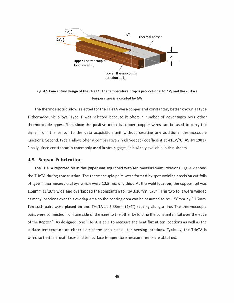
Fig. 4
The th
T thermo
thermoco
signal fro
junctions.
Finally, sin
4.5 SeThe T
the THeTA
of type T
1.58mm (
at many l
Ten such
pairs were
of the Kap
surface te
wired so t
4.1 Conceptua
hermoelectric
ocouple alloy
ouple types. F
om the senso
. Second, typ
nce constanta
nsor Fabr
THeTA reporte
A during cons
thermocoup
(1/16”) wide
ocations ove
pairs were p
e connected f
pton®. As des
emperature o
that ten heat
l design of the
c alloys select
ys. Type T w
First, since th
or to the da
e T alloys off
an is common
rication
ed on in this
struction. The
le alloys whic
and overlapp
r this overlap
placed on on
from one side
signed, one T
on either sid
fluxes and te
e THeTA. The t
temperatur
ted for the TH
as selected
he positive m
ata acquisitio
er a compara
nly used in str
paper was eq
e thermocoup
ch were 12.5
ped the const
p area so the
ne THeTA at
e of the gage
THeTA is able
e of the sen
en surface tem
45
temperature d
re is indicated
HeTA were co
because it o
metal is copp
on unit with
atively high Se
rain gages, it
quipped with
ple pairs wer
microns thic
tantan foil by
sensing area
6.35mm (1/4
to the other
e to measure
sor at all ten
mperature me
rop is proport
by V2
opper and co
offers a num
per, copper w
out creating
eebeck coeff
is widely ava
h ten measure
e formed by
ck. At the we
y 3.16mm (1/
can be assum
4”) spacing a
by folding th
the heat flux
n sensing loc
easurements
tional to V1 an
nstantan, bet
ber of advan
wires can be
any additio
icient at 41 V
ilable in thin
ement locatio
spot welding
ld location, th
/8”). The two
med to be 1.5
long a line. T
e constantan
x at ten locat
cations. Typic
are obtained
nd the surface
tter known as
ntages over
used to carr
nal thermoc
V/oC (ASTM 1
sheets.
ons. Fig. 4.2 s
g precision cu
he copper fo
foils were w
58mm by 3.16
The thermoc
n foil over the
ions as well a
cally, the THe
d.
e
s type
other
ry the
ouple
1981).
shows
t foils
il was
elded
6mm.
ouple
e edge
as the
eTA is

Fig. 4.2 TH
One c
to the dat
heat flux
thermally
same epo
between
foils from
materials
tunnels. F
painted u
discussed
4.6 Th
HeTA during c
constantan an
ta acquisition
measureme
y activated ep
oxy. These tw
two sheets o
m oxidation. S
. Finally, enc
Fig. 4.3 is a d
sing Zynolyte
in this paper
Fig. 4.3 Com
heoretical
onstruction. S
nd twenty co
n system. The
ents. Once w
poxy. The en
wo processes
of Teflon. En
Second, the
capsulating th
drawing of th
e flat black pa
r was calibrat
mpleted THeTA
Sensitivit
pot welded th
opper extensi
e extension w
welded and f
ntire gage wa
s were accom
capsulating t
Mylar isolate
he gage wate
he completed
aint if it will b
ed in radiatio
A wire for 10 h
ty and Tim
46
hermoelectric f
on wires wer
wires were so
folded, the f
as also encap
mplished sim
the gage serv
es the gage
erproofs it, a
d gage after e
e used to me
on, it received
eat flux and su
me Respons
foils are folded
re used to ca
oldered to the
foils were bo
psulated in 3
multaneously
ves multiple
electrically, a
allowing it to
encapsulation
easure a radia
d the black co
urface temper
se
d over Kapton
rry the signa
e foils at the
onded to th
3 micron thic
in a hot pre
purposes. Fir
allowing its u
o be used in
n. As a final s
ative heat flux
oating.
rature measure
resistance ba
ls from the T
edge opposit
e Kapton us
k Mylar usin
ess with the
rst, it protect
use on condu
research in w
step, the sen
x. Since the s
ements
rrier.
THeTA
te the
sing a
ng the
gage
ts the
uctive
water
nsor is
ensor
47
The sensitivity of the THeTA is dependent on the Seebeck coefficient of the thermoelectric materials
used and the thermal resistance of the resistance layer between the thermocouple junctions.
Multiplying these two parameters gives the theoretical sensitivity of the sensor.
"THeTAS Se R Sek
4.2
Fig. 4.4 shows a slice of the THeTA along with a model of its electrical analog circuit. For the
sensitivity estimations only the resistances are needed. The capacitances are later used to determine
the theoretical time response of the sensor. For the THeTA, the thermal resistance in Eq 4.2 (R”) is the
combined thermal resistance of the three layers between the two thermocouple layers. From Fig. 4.4 R”
is the resistance of the Kapton® plus the resistance of the glue layer on either side of the Kapton. The
resistances of the thermocouple layers are neglected because they are more than two orders of
magnitude smaller than any of the other layers.
" 2 G KR R R 4.3
Each individual resistance is simply the ratio of thickness to thermal conductivity. Based on
measurements of the Mylar, Kapton®, and welded foils, the thickness of the glue layer was estimated
from measurements of the average completed gage thickness. By assuming that all four glue layers were
the same thickness, the glue layer was determined to be approximately 20 microns thick. The thermal
conductivity of the epoxy was assumed to be 0.20 W/(m K) based on the measurements of Tanaeva and
Evseeva (Tanaeva and Evseeva 1997). The thickness of the Kapton® was measured to be 50 microns and
Dupont reports a thermal conductivity of 0.12 W/(m K) for type HN Kapton®. Adding these individual
resistances gives R”=6.167E 4 K/(W/m2). Multiplying the thermal resistance by the room temperature
Seebeck coefficient (41 V/oC) gives a theoretical sensitivity of 25.3 V/(kW/m2).

The ti
diffuse th
shown in
each laye
circuit, ea
was conce
used to s
flux.
Solvin
flux meas
ime response
rough the se
Fig. 4.4 was
er is the prod
ach layer was
erned, the en
olve the resu
ng the couple
ured by the g
Fig. 4.4 Cross
e of different
nsor and esta
used to dete
duct of the l
s treated as a
ntire layer wa
ulting set of e
ed equations
gage is then:
s sectional view
ial heat flux s
ablish a linea
ermine an est
ayer’s thickn
a lumped cap
as at a uniform
eight coupled
gives the te
48
w of THeTA an
sensors depe
r temperatur
timate of the
ness, density,
pacitance. Th
m temperatu
d ordinary dif
mperature hi
nd its electrical
ends on how
re profile with
THeTA’s tim
and specific
erefore, as fa
re. A fourth o
fferential equ
istory at each
l analogy
long it takes
hin the senso
e response. T
c heat. In the
ar as the the
order Runge
uations for a
h node in the
thermal ener
or. The RC net
The capacitan
e electrical a
rmal storage
Kutta method
step input in
e circuit. The
rgy to
twork
nce of
nalog
term
d was
n heat
e heat

49
1 2( ) ( )""
T t T tq tR
4.4
To determine the time response of the sensor, the ratio of the measured heat flux to heat flux input
(q”in) was examined. This ratio was found to be within 10% of a first order exponential response (1 e t/ )
for all t > 0.014s. Therefore, the sensor can be approximated as a first order system in the timeframe of
interest. The time required for the ratio to equal .632 ( ) was found to be 162 milliseconds.
4.7 Sensor CalibrationIn order to confidently use any heat flux sensor, it must first be accurately and thoroughly
calibrated. As a first calibration, the Seebeck coefficient of the thermoelectric alloys used was
determined experimentally. Next, the THeTA was calibrated in both conduction and radiation using RDF
and Schmidt Boelter reference sensors respectively. The radiation calibrations were further used to
experimentally determine the time response of the sensor. The THeTA was then analyzed in convection
by affixing it to a plate which experienced Hiemenz stagnation flow in a low speed water tunnel. Since
the THeTA measures both heat flux and surface temperature, it was used to measure the heat transfer
coefficient which was then compared to the analytical solution for Hiemenz flow. Finally, the Hybrid
Heat Flux (Hubble and Diller 2010) method was applied to the THeTA measurements to demonstrate
how the capabilities of such a sensor can be increased. The results of the calibrations are summarized in
Table 4.1 at the end of this section and an uncertainty analysis is presented in section 4.9 for each set of
calibrations.
4.7.1 Seebeck Coefficient Measurement
Since a traditional bulk wire thermocouple was not used in the manufacture of the THeTA, the
Seebeck coefficient of the copper/constantan foils was measured. This measurement was made by
affixing the THeTA to an aluminum plate equipped with a resistance heater. A type E thermocouple was
embedded in the aluminum plate and served as the temperature reference. The reference
thermocouple came supplied with a voltage to temperature polynomial and a quoted accuracy of 0.5oC.
A 24 bit National Instruments (NI) USB 9161 thermocouple DAQ was used to measure the voltages from
the THeTA as well as the type E standard at 1Hz. Since all temperature measurements were made
relative to room temperature, no cold junction compensation was needed. Prior to running a test, the
aluminum plate was wrapped in fiberglass insulation to minimize heat losses to the surroundings. The

50
plate was then heated to 10, 20, and 30 degrees above room temperature and allowed to reach steady
state. Once steady conditions were reached, the voltages produced between the constantan and copper
foils were measured and averaged over 5 minutes (300 samples). The Seebeck coefficient was then
determined by dividing this average voltage by the measured temperature rise. This calculation yielded
a Seebeck coefficient of the copper/constantan foils of 34.29±0.64 V/K which is somewhat lower than
the value typically associated with type T thermocouples. Using this value in place of the 41 V/K value
from section IV decreases the predicted sensitivity to 21.2 V/(kW/m2).
4.7.2 Conduction Calibration
The THeTA was calibrated in conduction using the conduction calibration facility located in the
Advanced Experimental Thermo fluids Engineering Research (AEThER) laboratory at Virginia Tech. This
system is described in detail in (Gifford, Hubble et al. 2010) and is shown in Fig. 4.5. One dimensional
conduction is maintained between two aluminum plates, one heated and the other cooled. An RDF
Corp. heat flux sensor (HFS 20455 1) was used as a reference as it has approximately the same thermal
resistance as the THeTA. The RDF sensor and the THeTA were placed in a mask of 75 micron thick
Kapton® HN the size of the plates in the conduction calibration facility as shown in Fig. 4.5. Above and
below the Kapton® layer, a layer of conformable Gap Pad© was used to minimize contact resistance.
This layer also served to make the overall resistance between the top and bottom plates more uniform.
For example, even though the overall resistance of the THeTA, RDF sensor, and Kapton® vary by up to
40%, once placed in series with two layers of the Gap Pad© ( =2E 3m, k=1W/mK) the thermal
resistance was uniform to within 5% over the area of the plates. Therefore, it was assumed that the heat
flux through the RDF sensor was within 5% of the heat flux through the THeTA. Once the stack was
assembled, it was insulated to help ensure that only conduction from the hot plate to the cold plate
occurred.

Fig. 4.5 Ste
Condu
controlled
from the
(Ewing 20
connected
as the out
To de
the calibr
STHeTA was
had reach
eady state con
uction calibra
d by varying
THeTA were
006). These a
d to a PC. A 2
tput of the ty
etermine the
ated output o
s averaged ov
hed steady sta
nduction calibr
ations were p
the voltage t
e amplified u
amplified sig
24 bit NI USB
ype T thermoc
sensitivity of
of the referen
ver 5 minute
ate.
ration facility.
the low
performed at
to the resista
using custom
nals were th
B 9161 therm
couple built in
f the ten sens
nce sensor.
THeS
es (300 samp
51
Heat flux is m
wer cooled plat
three levels
ance heater
amplifier bo
hen recorded
ocouple DAQ
nto the RDF.
sors on the T
THeTATA
ref
ref
VV
S
les) after the
maintained betw
te.
of heat flux,
on the hot p
oards whose
at 10Hz usi
Q was used to
Both RDF sign
THeTA, each s
e measured h
ween the upp
5, 10, and 15
plate. The ten
design is de
ng a 16 bit N
o record the R
nals were sam
sensor’s outp
heat flux and
er heated palt
5 kW/m2. Thi
n heat flux s
escribed by E
NI USB 6225
RDF output a
mpled at 1Hz.
put was divid
RDF temper
te and
s was
ignals
Ewing
DAQ
s well
.
ed by
4.5
rature

52
Fig. 4.6 Conduction calibration results with 95% confidence uncertainty and theoretical prediction
To demonstrate the repeatability of the conduction calibrations, the THeTA was calibrated at three
heat flux levels, removed from the calibration stand, the Gap Pad© replaced, and the three tests
repeated giving 6 total measurements of the sensitivity of the ten sensors. Fig. 4.6 shows the measured
sensitivities, the 95% confidence uncertainty estimates, and the theoretical sensitivity calculated using
Eq. 4.2. The estimated uncertainty was approximately 9% for the absolute heat flux calibration, the
majority of which is from uncertainty in the heat flux that is actually supplied to the gage. Repeatability
of all the measurements was better than this. Absolute heat flux calibrations at the national fire
research labs gave variations of up to ± 17% (Pitts, Murthy et al. 2006) demonstrating the difficulty in
absolute heat flux calibrations. The observed sensor to sensor variation shown in Fig. 4.6 is likely due to
the non uniform thickness of the glue layer, a parameter which proved difficult to control during
manufacture. Fig. 4.7 demonstrates how the thickness of the sensor affects its sensitivity by plotting
these two parameters against each other. With the exception of one outlier, the data shows a positive
correlation between sensor thickness and sensitivity.

53
Fig. 4.7 Sensitivity dependence on sensor thickness
4.7.3 Radiation Calibration
Radiation calibrations were performed using a halogen lamp as a radiation source. Equipped with a
600 watt halogen lamp, the radiation facility focuses the radiant energy using an elliptical reflector
which was machined from aluminum. The reflector was turned on a lathe and designed to have a focal
point 31.7mm (1.25 inches) from its end with heat fluxes up to 200kW/m2 obtainable. The radial heat
flux distribution of the lamp at an axial location corresponding to the focal point of the reflector was
characterized using a Vatell Corp. Heat Flux Microsensor (HFM 7) mounted on a 2 D traverse. The HFM
reference sensor averages the heat flux over an area approximately 3mm in diameter. Fig. 4.8 shows the
measured heat flux distribution and demonstrates that the heat flux is uniform to within 5% as long as
the sensor is not more than 5mm from the centerline of the reflector. As previously stated, the sensing
area of the THeTA is approximately 1.5mm by 3mm so the heat flux produced by the lamp can be
assumed uniform over the THeTA sensing area.
A variable transformer was used to control the AC voltage to the halogen lamp and allowed the level
of heat flux produced to be controlled. A Fluke 177 True RMS Multimeter with a quoted accuracy of 1%
of reading was used to measure the RMS voltage supplied to the lamp. A Schmidt Boelter water cooled
heat flux sensor (Medtherm model # GTW 7 32 485A) was used to calibrate the lamp and produce a
curve which related the heat flux produced to the voltage supplied. The reference sensor was painted
using the same Zynolyte flat black paint as was the THeTA for testing so there was no need to correct for
emissivity mismatches. It was found that if the lamp was left on for more than about thirty seconds the
reflector heated up enough to begin emitting additional radiation which caused the incident radiation to

54
the sensor to increase slightly with time. This problem was negated by placing a piece of standard plate
glass between the lamp and the test sensor. Since the glass was nearly opaque in the far infrared, it
blocked most of the radiation emitted by the reflector while still passing a large portion of the radiation
from the much hotter lamp. Tests showed that with the glass in place, the incident radiation increased
by less than 1% during the first 30 seconds of a test.
Fig. 4.8 Lamp radiation intensity as a function of radial location
Before the THeTA was calibrated in radiation, it was heat sunk by adhering it to an aluminum plate
using the same thermally activated epoxy used in its construction. The calibrations were then completed
by mounting the halogen lamp on a 2 D traverse in front of the sensor so that its position could be
accurately controlled. A jig was constructed to aid in the positioning of the lamp and allowed the lamp’s
position relative to the sensor to be accurate to within 0.25mm. A shutter system was designed to
subject the sensor to a step change of heat flux and consisted of a pneumatic cylinder which quickly
removed a piece of sheet metal from between the lamp and the sensor. Once the lamp had been turned
on and allowed to reach steady state (1 2 seconds), the cylinder removed the shutter. Two photodiodes
were used to determine the speed of the shutter as it passed the sensor. These tests showed that the
shutter was traveling at approximately 3.8 m/s and therefore uncovered the sensor in about 400
microseconds which is more than two orders of magnitude faster than the predicted response of the
sensor. Therefore, the incident radiation can be treated as a perfect step input for analysis. Fig. 4.9 is a
depiction of the radiation calibration facility.

Each
kW/m2. T
calibratio
Fig
determine
approxim
determine
the senso
(5000 sam
Fig. 4.10
theoretica
very good
Fig. 4.9 Radiat
individual se
The signals fr
ns except tha
g. 4.10 Radiatio
e the time re
ately ten sec
e the sensor’
ors. The sensi
mples) by the
shows the
al sensitivity c
d agreement,
tion calibratio
nsor on the T
om the THeT
at the signals
on calibration
esponse and
conds. The da
s time respo
tivities were
heat flux abs
measured s
calculated us
far better th
n setup. Shutt
THeTA was ca
TA were reco
were sample
results with 9
to acquire e
ata recorded
nse while the
determined
sorbed by the
sensitivities,
ing Eq. 4.2. N
an the estima
55
ter utilized to p
alibrated at h
orded using t
ed at 1kHz. It w
95% confidence
enough data
during the fir
e last 5 secon
by dividing th
e Schmidt Bo
the 95% co
Note that for e
ated absolute
provide a step
heat fluxes of
the same har
was necessar
e uncertainty a
for averaging
rst 500 millis
nds was used
he sensor’s o
elter with the
onfidence un
each sensor t
e uncertainty
p change in inc
f approximat
rdware used
ry to sample a
and theoretica
g since the to
econds of the
to determine
utput averag
e lamp set at
ncertainty es
the measured
(95% confide
ident flux
tely 10, 15, a
in the condu
at a higher ra
al prediction
otal test time
e test was us
e the sensitiv
ged over 5 sec
the same vo
stimates, and
d sensitivities
ence) of 8% s
nd 20
uction
te to
e was
sed to
vity of
conds
ltage.
d the
show
hown

by the err
are used
large chan
of hot pre
layers.
To est
used whic
Plotti
is behavin
vs. t. The
approxim
estimatio
output to
fit to the
determine
constant v
IV).
ror bar. Radia
more often fo
nge in sensiti
essing the TH
Fig
timate the tim
ch utilizes the
ng the left ha
ng as a first or
near linear
ately a first o
n compared
reach some
e data. Using
ed as reporte
value of 168
ation calibrat
or heat flux c
ivity for senso
HeTA onto th
g. 4.11 Transien
me response
e mathematic
and side as a
rder system.
behavior of t
order type. T
to the alter
threshold. To
g the slope f
ed in the tab
milliseconds
tions are gene
calibrations (M
ors 5 and 7 (
he aluminum
nt response of
of the THeTA
cal first order
ln 1 out
in
function of t
Fig. 4.11 and
the curve in
This approxim
native appro
o determine t
from the line
le at the end
compares w
56
erally more r
Murthy, Tsai
34% and +20
plate which
f THeTA to ste
A, the metho
exponential
lnt
e
produces a li
Fig. 4.12 sho
Fig. 4.12 is a
mation in tur
oach of deter
the slope of t
ear regressio
d of the calib
well with the p
repeatable th
et al. 2000).
0% respective
altered the r
p radiation he
d outlined by
response to a
1 t
inear curve w
ow the sensor
an indication
rn leads to a
rmining the t
he curve in F
n, the time
ration sectio
predicted val
an conductio
It is believed
ely) was caus
relative thick
eat flux input
y Doebelin (D
a step change
with a slope o
r response as
that the sen
more accura
time required
ig. 4.12, a line
constant for
n. The avera
ue of 162 mi
on calibration
that the rela
sed by the pr
nesses of the
Doebelin 2004
e input.
of 1/ if the s
well as ln(1 q
sor is behavi
ate time resp
d for the sen
ear regressio
each senso
ge measured
lliseconds (se
ns and
atively
rocess
e glue
4) was
4.6
ensor
q0/qin)
ing as
ponse
nsor’s
n was
r was
d time
ection

57
Fig. 4.12 Time response of the logarithmic heat flux and least squares fit. Fit used to measure first order time
constant
4.7.4 Hybrid Heat Flux Analysis
A recent paper by the authors (Hubble and Diller 2010) discusses a procedure called the Hybrid Heat
Flux (HHF) method for increasing the performance of differential heat flux sensors. During transient
tests, the heat flux flowing through the gage will be different to that flowing into the gage. By
accounting for the heat stored by the gage in conjunction with the heat flowing through the gage, the
accuracy and time response of a differential heat flux sensor can be improved. In order to apply this
method, an extra calibration is needed to determine the thermal mass per unit area of the sensor. This
value can be determined by mounting the sensor on an insulating material and subjecting it to a known,
radiative heat flux. The thermal mass per unit area ( C ) is then measured as the inverse of the slope of
the temperature history curve. Values of 680 to 710 J/(m2K) were measured for the ten sensors on the
THeTA. The HHF method is then applied as follows:
1" " "2HHF Diff Slugq q q 4.7
where q”Diff is the heat flux measured treating the THeTA as a differential sensor and q”Slug is the value
measured treating the THeTA as a slug calorimeter. In this case, the slug calorimeter term uses the
average temperature measured by the THeTA:

Fig. 4
presented
overshoot
correspon
attenuatio
Fig.
4.7.5 C
Table
calculatio
4.13 shows a
d in Fig. 4.14.
t. Here, the
nds to resolvi
on.
4.13 Hybrid he
alibration S
4.1 summar
n are provide
Sens
1234567
a plot of the
. A dramatic
95% time re
ing sinusoida
eat flux respon
Summary
rizes the res
ed in section 4
Table
sor SHF
V/(k
1121222
"Slugq
HHF metho
increase in ti
esponse is im
al signals with
nse of THeTA t
ults of the s
4.9.
e 4.1 Summary
FA Cond
kW/m2) V
19.419.024.419.226.322.023.0
58
1
2TdC
dt
od applied to
me response
mproved by
h frequencies
to step change
sensor calibra
y of THeTA cali
SHFA Rad
V/(kW/m2)
17.518.025.517.317.521.627.7
2
2T
o the radiatio
e is observed
a factor of 1
s up to 6.4Hz
e input compa
ation. Details
ibration result
TimeConstant
ms
172172208180176174165
on calibration
at the expen
14 from 509
z with less th
red to differen
s of the estim
ts
Thickness
microns
163150216155152196213
n data which
nse of a slight
9ms to 36ms
an 10% amp
ntial response
mated uncert
s
4.8
h was
t (3%)
. This
litude
tainty

59
8 17.4 17.5 144 1609 17.7 17.3 121 16310 19.3 20.2 173 193
Uncertainty 9% 8% 13% ±5
4.8 Example of Sensor Application
4.8.1 Steady Convection
Using the THeTA, convective heat transfer coefficients were measured in a low speed, low
turbulence (Tu < 1%) closed loop water tunnel. The aluminum plate to which the THeTA was mounted
was attached to a stagnation model which spanned the width of the water tunnel’s 0.61m square test
section. The stagnation model measured 0.152m square by 0.61m wide and was equipped with an aft
splitter plate to prevent vortex shedding interactions with the stagnation region. The THeTA was
positioned horizontally such that all 10 sensors fell along the stagnation line. Using the resistance heater
that was adhered to the back of the aluminum plate, the central, thermally isolated, test area was
heated approximately 15oC above the water temperature. Flow measurements were made along the
stagnation line directly upstream of the THeTA using Time Resolved Digital Particle Image Velocimetry
(TRDPIV)(Westerweel 1997). Fig. 4.14 shows the test setup. Tests were performed by allowing the
heated aluminum plate to reach steady state conditions while the tunnel was run at U=0.10m/s. The
convective heat transfer coefficient was measured by the THeTA using Newton’s Law of Cooling.
"qhT
4.9
T was measured using the surface thermocouples on the sensor and q” was determined using the
sensitivity found from the radiation calibrations. For comparison, an analytical value for h was
calculated. For stagnation flows, Goldstein (Goldstein 1938) gives a solution for the heat transfer
coefficient as
0.420.5421 Pr ah k 4.10
where k, , and Pr are the thermal conductivity, kinematic viscosity, and Prandtl number of the fluid
(water in this case). The parameter a is the spatial acceleration constant and was found experimentally
from the TRDPIV measurements to be a=0.98 s 1. This agrees well with the correlation given by White
(White 1974) for a square body in cross flow which relates the parameter a to the freestream velocity U
and the body height L.

Using
estimated
Goldstein
prediction
4.8.2 U
One o
a bounda
g Eq. 4.10 wit
d to be 757 W
’s prediction
n.
Fig. 4.14 Set
Fig. 4.15
Unsteady Con
of the purpos
ry layer and
th the fluid p
W/m2K. Fig. 4
. On average
tup for convect
5 Comparison o
nvection
es for the de
their subseq
a
properties at
4.15 shows t
e, the THeTA
tion analysis. H
of measured a
velopment of
quent transien
60
1.032
UL
the film tem
he compariso
A measureme
Hiemenz flow
and predicted h
f the THeTA w
nt effect on t
mperature, the
on of the me
nt is about 1
produced in a
heat transfer c
was to study
the convectiv
e heat transf
easured value
10% higher t
a water tunnel
coefficient valu
the interactio
ve heat trans
fer coefficien
es of h along
han the anal
facility.
ues.
on of vortices
sfer coefficien
4.11
t was
g with
lytical
s with
nt. To

study this
impinge n
the flow
measured
4.9) allow
obtained
ring impa
coefficien
measurem
measured
shown. W
indicating
4.9 UnThe fo
in conduc
Steele 198
s phenomena
normally on t
field directly
d the heat flux
wed the time
from the exp
acts the plat
nt measured b
ments are ma
d flow field. T
When the vor
g an h value o
Fig
ncertainty
ollowing unce
ction and rad
89). The total
a, a vortex rin
the heated pl
y in front o
x and surface
resolved hea
periment. On
te after prop
by the THeTA
ade at the te
he vertical lin
rtex ring arriv
of more than 2
g. 4.16 Sensor
y Analysis
ertainty analy
diation and fo
l uncertainty
US
ng (Shariff and
ate to which
f the sensor
e temperature
at transfer co
the left is the
pagating from
A normalized
en locations
ne indicates t
ves, the heat
2000 W/(m2K
application, v
ysis was perf
ollows the p
in the THeTA
2
1
THeTAj
S
iTHeTA
US
61
d Leonard 19
the THeTA w
r while the T
e at ten point
oefficient to
e flow field as
m the left. T
by the natur
indicated by
he time corre
t transfer coe
K).
vortex ring imp
ormed on the
rocedure out
A sensitivity, S
1
1 T
THeTA
SS X
992) was gene
was mounted
THeTA (with
ts. Combining
be determine
s measured b
The plot on
ral convectio
y the dots at
esponding to
efficient incr
pinging on a he
e calculation
tlined by Col
STHeTA, for a pa
2
i
THeTAX
i
UX
erated in wat
d. TRDPIV was
HHF applie
g these two m
ed. Fig. 4.16
by the TRDPIV
the right is
n value of 51
the right ed
the instantan
eases by ove
eated plate.
of the sensit
eman and St
articular meas
ter and allow
s used to me
d) simultane
measurement
shows the re
V just as the v
the heat tra
10 W/(m2K). T
dge of the TR
neous TRDPIV
er a factor of
tivity of the T
teel (Coleman
surement is
wed to
easure
eously
ts (Eq.
esults
vortex
ansfer
These
RDPIV
V field
f four
THeTA
n and
4.12

62
where UsTHeTA is the total experimental uncertainty, which is a function of experimental variables Xi. The
total 95% uncertainty in each variable is given by Uxi, while the partial derivatives are the associated
sensitivity coefficients. Uxi is estimated or calculated by combining variable’s precision and bias error
limits. Bias limits for the DAQs, thermocouples, and reference sensor were provided while precision
limits were calculated from 128 continuous samples of nominal room temperature data using a
Student’s t distribution with a 95% confidence interval. Plugging Eq. 4.5 into Eq. 4.12 gives the
uncertainty of the sensitivity found in conduction.
2 222THeTA
THeTA Cond
V Vref SrefS THeTA rep
THeTA ref ref
U U UU S U
V V S4.13
where Urep is the estimated bias error in the repeatability of the conduction calibration facility and is
estimated at 5%. Uncertainty calculations for radiation calibrations are performed in the same manner
as shown in Eq. 4.14.
2 2"
"THeTA
THeTA Rad
V qS THeTA
THeTA
U UU S
V q4.14
where Uq” is a combination of the error in the voltage reading supplied to the lamp and the error in the
curve generated from the Schmidt Boelter data. The total error in the conduction calibrations was
determined to be approximately 9% while the radiation calibrations yielded an uncertainty of 8%.
To determine the uncertainty in the time constant estimation, a sequential perturbation method
was used as outlined by Moffat (Moffat 1985). This method essentially uses finite differences to
estimate the relative sensitivities of the time constant calculation to each measured variable. After some
simplification, the time constant can be expressed as
1
0
0
ln 1SS
V Vddt V V
4.15
where V is the measured voltage from the sensor, V0 is the measured voltage offset, and VSS is the
measured voltage once the sensor reached steady state. Since the term inside the parentheses should
be linear, the temporal derivative was estimated by the slope of a linear regression fit to the data. Each
independent variable (V, Vo, and VSS) was then perturbated independently by its respective uncertainty
to determine the uncertainty contributions from each variable. These individual uncertainties were then

63
combined to determine the overall uncertainty for the time constant calculations. Averaging the
uncertainties for the 10 sensors yielded an overall uncertainty of 13%.
4.10 ConclusionsThe THeTA offers improved performance compared to currently available heat flux sensors. The use
of thermoelectric foils results in a durable, sensitive transducer. In addition to measuring heat flux, the
THeTA is capable of measuring simultaneous surface temperatures which allows it to more completely
describe the thermal environment. Temperature measurements are also used in the HHF method to
increase the performance of the sensor. The resulting time resolved heat flux and temperature
measurement capabilities make the THeTA very useful in a variety of research and practical applications.
The capabilities of the THeTA were demonstrated by conduction and radiation calibrations as well as an
example of the THeTA measuring the time resolved convective heat transfer coefficient resulting from a
transient flow field.
4.11 AcknowledgmentsThis material is based upon work supported by the National Science Foundation under Grant No.
CTS 0423013. Any opinions, findings, and conclusions or recommendations expressed in this material
are those of the authors and do not necessarily reflect the views of the National Science Foundation.

64
5 A Hybrid Method for Heat Flux Measurement
David O. Hubble and Tom E. Diller
Published in the ASME Journal of Heat Transfer, Vol. 132, Dec 2010
5.1 AbstractThe development and evaluation of a novel hybrid method for obtaining heat flux measurements is
presented. By combining the spatial and temporal temperature measurements of a heat flux sensor, the
time response, accuracy, and versatility of the sensor is improved. Sensors utilizing the hybrid method
are able to make heat flux measurements on both high and low conductivity materials. It is shown that
changing the thermal conductivity of the backing material four orders of magnitude causes only an 11%
change in sensor response. The hybrid method also increases the time response of heat flux sensors.
The temporal response is shown to increase by up to a factor of 28 compared to a standard spatial
sensor. The hybrid method is tested both numerically and experimentally on both high and low
conductivity materials and demonstrates significant improvement compared to operating the sensor as
a spatial or temporal sensor alone.
5.2 Nomenclature
C = specific heat Fo = Fourier number, t / 2
k = thermal conductivity h = convective heat transfer coefficient q" = heat flux q0" = step change heat flux for simulation q1" = heat flux into sensor face
q2" = heat flux out of sensor back
q"Differential = heat flux measured by differential sensor
q"HFM = heat flux measured by HFM reference sensor
q"Slug = heat flux measured by slug calorimeter
t = time
tss = time to reach steady-state T1 = temperature at sensor face T2 = temperature at sensor back Tave = average sensor temperature

65
Tr = measured jet recovery temperature TS HFM = HFM surface temperature TS HTHFS = HTHFS surface temperature T = room temperature x = distance from sensor face
= thermal diffusivity of sensor, k/ C t = time between temperature measurements, inverse of sampling frequency = thickness of sensor
= density
5.3 IntroductionModeling of thermal systems requires a combination of temperatures and energy fluxes for
prediction of their performance. Temperatures are commonly measured by a variety of standard
methods, but the measurement of heat flux is a particular challenge because it is an energy flux normal
to a plane of material rather than a property of a material. Therefore, sensors to measure heat flux
usually must be mounted onto a material that provides a good heat sink so that the energy flow is not
impeded. This makes it very difficult to use heat flux gages to measure heat flux on materials that are
not good thermal conductors. The purpose of this paper is to present a new method which allows heat
flux gages to make accurate measurements on any type of backing material. Applications include
furnaces to thermal protection systems for spacecraft.
5.4 BackgroundTwo of the most common modes of heat flux measurement are that of a differential heat flux sensor
and that of a slug calorimeter (Diller 1993). A differential heat flux sensor measures the temperature
difference over a spatial distance with a known thermal resistance, as illustrated in Fig. 5.1. The
temperature difference is used to calculate the heat flux through the sensor from the steady state
version of Fourier’s Law. T1 is the temperature of the exposed face while T2 is the temperature at the
back of the sensor.
" 1 2Differential
T Tq k 5.1
Under steady state conditions the heat flux entering the sensor in Fig. 5.1, q1", is equal to that leaving,
q2". Hager (Hager 1965) calculated the 98% response time to a step change of heat flux at the surface in
terms of the sensor’s thickness and thermal diffusivity. This is often considered as steady state.

Hager’s (H
sink wher
In a s
function
capacitan
the senso
where C
all sensor
Eq. 5.3 w
measure t
temperat
short tim
slug’s ave
delay bef
change of
Hager 1965)
re the backsid
Fig. 5.1 S
slug calorime
of time. The
ce is known.
or “slug” yield
C is the therm
r surfaces exc
would perfect
the average t
ure at the ba
e after a hea
erage temper
fore the slug
f heat flux at t
analysis was
de temperatu
ensor backing
eter the amo
e rate of ch
As illustrated
s
mal mass of t
cept for the s
tly measure t
temperature,
ck surface is
at flux is app
rature is incre
accurately m
the surface is
sst
performed o
re, T2, remain
g system. T1 an
ount of ther
hange of the
d in Fig. 5.1, c
Slug"q C
the slug per s
sensor face. I
the net heat
, the slug is t
used to appro
plied to the s
easing) befor
measures the
s given as
66
21.5s
on the ideal c
ns constant.
nd T2 are the tw
mal energy a
e sensor’s te
conservation
avedTC qdt
ensor area. T
f the average
flux into the
ypically made
oximate the s
slug, thermal
re any heat h
actual net h
case of a sens
wo sensor surf
absorbed by
emperature
of energy fo
1 2" "q q
The heat loss
e temperatur
e slug. Howe
e from a high
slug’s average
energy is be
has reached t
heat flux. The
sor mounted
face temperatu
the sensor
is measured
r a control vo
(q2") is minim
re within the
ever, since it
h conductivity
e temperatur
eing absorbed
the back surf
e 99% respon
on a perfect
ures.
is measured
d and its the
olume surrou
mized by insu
slug were kn
is not possib
y material an
re. Therefore,
d by the slug
face. This cau
nse time to a
5.2
t heat
as a
ermal
nding
5.3
lating
nown,
ble to
nd the
, for a
g (the
uses a
a step

67
20.54sst 5.4
by Hightower et al. (Hightower, Olivares et al. 2008). This analysis was performed assuming a perfectly
insulated backside surface (q2"=0).
While these two modes of operation can be used for specific measurement applications, they both
have serious limitations. For example, for a differential gage to have a fast time response, it must be
very thin. This is difficult to achieve in harsh environments where sensors typically must be made with a
substantial thickness to survive. Also, since a differential sensor only measures heat flowing through it, it
must be provided with a good heat sink. This necessitates its mounting on or in a high conductivity
material, not an insulator. The main problems encountered when using a slug calorimeter include
adequately insulating the slug to minimize losses as well as noise amplification due to the differential
operation. Also, since the output of a slug is proportional to the rate at which its temperature is
changing, it is unable to measure a heat flux at steady state. It is worth noting that the design criteria for
these two types of sensors are opposite. A differential gage more accurately measures q1" when q2" is
maximized with minimal heat storage in the gage. Conversely, a slug calorimeter needs to minimize q2"
and maximize the stored thermal energy.
A number of papers have reported using a combination of the spatial and temporal changes of
temperature to infer or improve heat flux measurements. Kidd and Adams (Kidd and Adams 2001) used
finite element analysis to determine a response function for their Schmidt Boelter heat flux gages. This
was used to compensate for the energy deficit caused by the thermal capacitance of this differential
style gage. They were able to substantially increase the time response of the heat flux measurements for
their transient tests in high speed wind tunnels. A complete analysis of a simpler thin polyimide
differential gage mounted on a metal heat sink was performed by Epstein et al. (Epstein, Guenette et al.
1986). This enabled measurements from steady state to 100 kHz on metal turbine blades, but required
solution of the equations for one dimensional transient conduction for a particular mounting material. A
“plug type heat flux gauge” was developed by Liebert (Liebert 1992) to account for the combination of
conduction and storage in the post normal to the surface. Four temperatures were measured along the
post as a function of time and compared with transient temperature solutions to determine the surface
heat flux. Experimental results were obtained for metal turbine blade models. Unfortunately, the
method did not work well when the sensor was mounted in a low thermal conductivity material (Rooke,
Fralick et al. 1998).

68
A popular variation of the slug calorimeter uses a single temperature measurement at the surface of
the material and a semi infinite solution to the transient thermal field. The results can be used only over
a short time span before the thermal front reaches the backside of the material, which corresponds to
the time before results from a slug calorimeter can be used. The data reduction procedure involves
inverse solution methods because the measured surface temperature is the known boundary condition
that is used to solve for the corresponding heat flux. Several digital and analogue processing methods
have been developed in efforts to minimize the effect of noise in the resulting heat flux signal (Schultz
and Jones 1973; George, Rae et al. 1991; Walker and Scott 1998). There are a number of methods
available for measuring the transient surface temperature. Point measurements can be made with
resistance temperature sensors (RTD’s) (Anthony, Jones et al. 2005) or coaxial thermocouples (Kidd,
Nelson et al. 1994). Optical methods include liquid crystals(Wang, Ireland et al. 1995), infrared
thermography(Nasir, Ekkad et al. 2007), and thermographic phosphors (Bizzak and Chyu 1995) that can
be used with high speed imaging cameras to scan over an entire surface. The biggest limitations are
that the initial temperature distribution throughout the material must be known, there are no steady
state results, and the test time is limited.
Clearly, there are advantages to including both the differential and transient slug type responses for
measuring heat flux. It would be beneficial to design a simple sensor and analysis scheme which could
utilize the advantages of these two sensor types together while minimizing their negative
characteristics. It is with this goal in mind that the following analysis was performed on a simple one
dimensional sensor for such a hybrid heat flux (HHF) method.
5.5 HHFMethodology
5.5.1 Differential Term.
Fig. 5.1 shows the schematic of a one dimensional heat flux sensor. The majority of differential heat
flux sensors are designed to minimize 2 D effects and can therefore be treated as one dimensional. The
quantity q1" represents the heat flux into the sensor face, which is the desired measurement. Fig. 5.2
depicts a typical temperature profile resulting from a heat flux, applied at the sensor face, which
diffuses through the sensor and into the backing material. These profiles will be non linear until the
entire system reaches steady state at which point both curves will become linear. Using Fourier’s law,
" dTq kdx
5.5
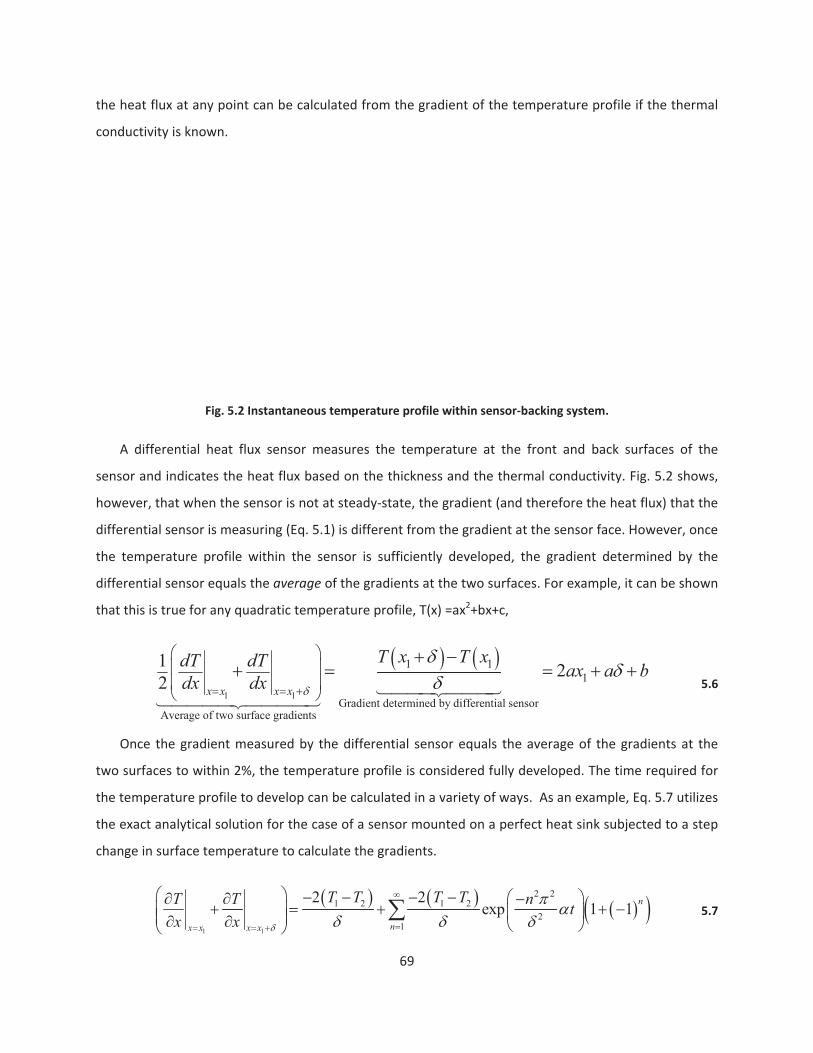
the heat f
conductiv
A diff
sensor an
however,
differentia
the temp
differentia
that this i
Once
two surfa
the tempe
the exact
change in
flux at any po
vity is known.
Fig. 5
ferential hea
nd indicates t
that when th
al sensor is m
perature prof
al sensor equ
s true for any
1
Average of two
12 x x
dTdx
the gradient
ces to within
erature profil
analytical so
surface temp
1x x
Tx
oint can be ca
5.2 Instantane
t flux sensor
he heat flux
he sensor is n
measuring (Eq
file within th
uals the avera
y quadratic te
1
o surface gradien
x x
dTdx
t measured b
n 2%, the tem
le to develop
lution for the
perature to c
1x x
Tx
alculated from
eous temperat
r measures t
based on the
not at steady
. 5.1) is differ
e sensor is s
age of the gra
emperature p
Gradient nts
T
by the differe
mperature pro
can be calcu
e case of a se
alculate the g
1 22 T T
69
m the gradie
ture profile wit
he temperat
e thickness an
state, the gra
rent from the
sufficiently d
adients at the
profile, T(x) =a
1
determined by d
T x
ential sensor
ofile is consid
lated in a var
ensor mounte
gradients.
1
1
2
n
T
nt of the tem
thin sensor ba
ture at the f
nd the therm
adient (and th
e gradient at t
eveloped, th
e two surfaces
ax2+bx+c,
1
differential senso
T x
equals the a
dered fully de
riety of ways.
ed on a perfec
2 expT n
mperature pro
acking system.
ront and bac
mal conductivi
herefore the
the sensor fa
e gradient d
s. For exampl
1
or
2ax a
average of th
eveloped. The
As an exam
ct heat sink s
2 2
2 1n t
ofile if the the
ck surfaces o
ity. Fig. 5.2 sh
heat flux) tha
ce. However,
determined b
le, it can be s
a b
e gradients a
e time require
ple, Eq. 5.7 u
subjected to a
1 n
ermal
of the
hows,
at the
, once
by the
hown
5.6
at the
ed for
tilizes
a step
5.7

70
The gradients at the two sensor surfaces are then compared to the gradient determined from the two
surface temperatures, (T2 T1)/ , to see when they agree to within 2%. For the analytical case described
by Eq. 5.7, a time corresponding to a Fourier number (non dimensional time, Fo = t / 2) of 0.12 is
required. The Fourier number required for the temperature profile to become fully developed was also
calculated analytically for a step change in heat flux on a perfect heat sink and was found to be 0.91.
Numerical simulations of cases other than a perfect heat sink show that a step change in heat flux on a
perfect heat sink requires the longest time to become fully developed. For a typical ceramic gage (Oishi,
Gorbunov et al. 2006) with a thickness of 500 m and thermal diffusivity of 1.0E 5 m2/s, a Fo of 0.91
corresponds to a time of 22.8 milliseconds. For a metallic sensor such as the High Temperature Heat Flux
Sensor HTHFS (Gifford, Hubble et al. 2010) with a thickness of 3.2mm and thermal diffusivity of 5.5E 6
m2/s a Fo of 0.91 corresponds to a time of 1.69 seconds.
Once the temperature profile is fully developed, Eq. 5.6 can be used to relate the heat fluxes q1" and
q2". The temperature gradients at the sensor face and back surfaces represent the heat flux into and out
of the sensor, respectively, and the differential sensor heat flux is proportional to the total temperature
difference, T1 – T2. Substituting the corresponding heat fluxes into Eq. 5.6 gives
1 "2 1 2Differential
" "2
q q T Tq k 5.8
5.5.2 Slug Term
A slug calorimeter measures heat flux by measuring the rate at which heat is absorbed by the slug.
The absorbed flux represents the net heat flux into the control volume, q1" q2", as shown in Fig. 5.2. Eq.
5.3 states that this net heat flux can be measured using a slug calorimeter which measures the time rate
of change of the slug’s average temperature. As mentioned, the standard method for measuring this
average temperature is to measure the temperature at the back of the sensor and assume that this
approximates the actual average temperature. This is a valid assumption once enough time has passed
for the heat that enters the sensor face to reach the sensor back. However, for the sensor shown in Fig.
5.1, both surface temperatures are known. By utilizing the temperature measurement at the sensor
face, a more accurate measure of the absorbed heat flux can be made. Subsequently, the sensor can be
operated as a slug calorimeter in three different modes; the sensor’s average temperature can be
approximated by the face temperature, the back temperature, or an average of the two. The response
of a slug calorimeter to a step change in heat flux while mounted on a perfect insulator using these

71
three methods is shown in Fig. 5.3. The sensor properties and the numerical method are discussed in
section 5.6.
Fig. 5.3 Comparison of slug calorimeter response using different sensor temperature measurements.
Fig. 5.3 shows that utilizing only the surface temperature offers no advantages compared to only
using the back temperature as it takes just as long for an accurate measurement to be made. On the
other hand, utilizing the average of the two surface temperatures has advantages and drawbacks. By
utilizing both the sensor face and back temperatures, the time response is more than a factor of three
faster compared to using only T2 but this temporal increase is accompanied by a large overshoot. The
overshoot associated with using T1 in the slug measurement is a result of the t dependence of the
surface temperature since the sensor acts as a semi infinite solid before heat has had a chance to reach
its back surface. Since the surface temperature history is a function of t , it has an infinite temporal
derivative at t=0. While the overshoot associated with using the average of the two surface
temperatures is initially large, it measures the applied heat flux more accurately than the standard
method (curve is closer to one) for all Fourier numbers greater than 0.02. Therefore, in many situations
it is advantageous to utilize the average of the two surface temperatures in order to increase the
temporal response of the sensor. From this point on, q"Slug will denote a slug calorimeter that utilizes the
average of T1 and T2 unless specified otherwise.
1 21 2
Slug " ""2
q qT Tdq C
dt 5.9
5.5.3 Hybrid Heat Flux

72
To combine the spatial and temporal responses of a heat flux sensor, only Eqs. 5.8 and 5.9 are
needed, as repeated here.
1 2 Differential" " 2 "q q q 5.10
1 2 Slug" " "q q q 5.11
Combining Eqs. 5.10 and 5.11, and solving for the desired q1" yields the HHF method.
1 Differential Slug1" " "2
q q q 5.12
Equation 5.12 shows how the differential and slug calorimeter outputs of a sensor can be combined.
While this represents a simple model, it was derived from basic thermal energy conservation.
The validity of Eq. 5.12 can be supported by examining two limiting cases. First, consider the limit of
a perfectly insulating backing material. For this case, the one dimensional heat equation within the
sensor simplifies to
2
2 Const.d Tdx
5.13
once the temperature profile is fully developed. The solution to this equation yields a temperature
profile within the sensor that is quadratic with a gradient of zero at x= since q2"=0. This means, using
Eq. 5.6, that the differential sensor will measure exactly half the heat flux entering the sensor. Also,
since q2" is zero for this case, the slug calorimeter will measure the heat flux perfectly, i.e. q"Slug =q1".
Therefore, the hybrid method described in Eq. 5.12 will measure the correct heat flux for this case.
Another limiting case occurs when the entire system is at steady state on a perfect heat sink
(d2T/dx2=0). For this case, the temperature profile within the sensor is linear. Consequently, the
differential sensor will measure the exact heat flux, q"Differential= q1". Also, since the system is at steady
state, the time derivative of the temperature everywhere in the sensor is zero and the slug calorimeter
will measure zero heat flux. Once again, the HHF method (Eq. 5.12) handles this limiting case.
The HHF method requires that a sensor be designed such that T1, T2, and T are measured.
However, accurately measuring any two of these allows the third to be calculated since T=T1 T2. For
the two sensors already mentioned (Oishi, Gorbunov et al. 2006; Gifford, Hubble et al. 2010) the hybrid

73
method can be used without any change in design since these two sensors already measure the
required temperatures.
5.6 HHF Numerical ValidationIn order to validate the HHF method, 1 D transient conduction through the sensor backing system
(Fig. 5.1) was modeled using finite difference computations. This was accomplished using an in house
developed code which utilizes an implicit discretization of the 1 D heat equation in MATLAB. The
derivation of this discretization can be found in (Incropera and DeWitt 2002). The boundary conditions
at the senor face allowed any thermal condition to be applied including time varying fluxes and
convective or radiative conditions. Temporal and spatial steps were kept sufficiently small to eliminate
any grid and time step dependence. This was verified for the parameters shown in Table 5.1 by
increasing both the temporal and spatial resolution by a factor of ten over the values in Table 5.1 and
comparing the results to those obtained using the lower resolution. In both cases, the discrepancy was
less than 0.1%. Changing material properties as well as the thickness of the sensor allowed for any
sensor design to be tested. Also, the material properties and thickness of the backing material could be
varied to investigate how this affected sensor performance. For all numerical simulations shown, the
HTHFS (Gifford, Hubble et al. 2010) (described in section 5) was modeled mounted on a backing material
three times thicker than the sensor. It was verified that the baking material thickness did not
significantly affect the analysis. This was done by varying the thickness from one to ten times the
thickness of the sensor which caused less than a 3% change in sensor performance. For all tests, the
boundary condition at the back surface of the backing material was held at a constant temperature.
Table 5.1 summarizes the parameters used in the numerical simulations.
Table 5.1 Parameters used in numerical simulation
Parameter Value Units
Sensor thermal conductivity 22 W/m K
Sensor density 7278 kg/m3
Sensor specific heat 548 J/kg K
Sensor thickness 3.175 mm

74
Backing thickness 9.525 mm
Backing thermal conductivity 0.22 to 2200 W/m K
Spatial step 0.03175 mm
Time step 0.5 ms
At each time step in the code, the temperatures at the face and back of the sensor (T1 and T2) were
recorded. This allowed the sensor’s performance in all three modes of operation to be evaluated using
only these two temperature histories along with the sensor’s properties. The sensor’s response to a step
heat flux of q0" is plotted against Fourier number (dimensionless time) in Fig. 5.4. A step change in heat
flux is used in all the numerical simulations because it allows for the most direct comparison between
different modes of sensor operation and backing conditions.
Fig. 5.4 Simulated response of sensor in three modes of operation. HHF method significantly increases sensor
performance.
In the analysis shown in Fig. 5.4, the properties of the backing material were identical to the
properties of the sensor. The accuracy as a slug calorimeter decreases with time while the differential
sensor’s accuracy increases with time. As the temperature of the sensor increases, more heat is
conducted through the sensor into the backing material (q2" is increasing). If steady–state conditions
were reached, the differential sensor would measure the exact heat flux. Because the backing material
in this case is identical to the sensor, the entire system acts as a semi infinite solid, which never reaches
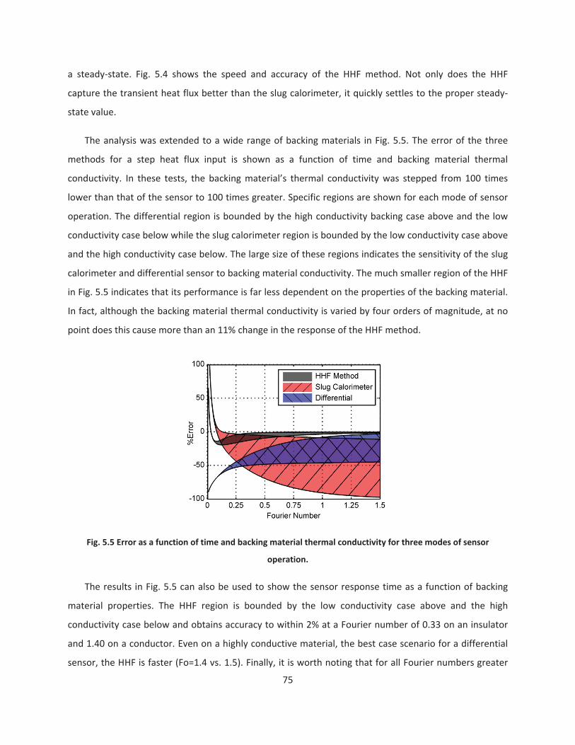
75
a steady state. Fig. 5.4 shows the speed and accuracy of the HHF method. Not only does the HHF
capture the transient heat flux better than the slug calorimeter, it quickly settles to the proper steady
state value.
The analysis was extended to a wide range of backing materials in Fig. 5.5. The error of the three
methods for a step heat flux input is shown as a function of time and backing material thermal
conductivity. In these tests, the backing material’s thermal conductivity was stepped from 100 times
lower than that of the sensor to 100 times greater. Specific regions are shown for each mode of sensor
operation. The differential region is bounded by the high conductivity backing case above and the low
conductivity case below while the slug calorimeter region is bounded by the low conductivity case above
and the high conductivity case below. The large size of these regions indicates the sensitivity of the slug
calorimeter and differential sensor to backing material conductivity. The much smaller region of the HHF
in Fig. 5.5 indicates that its performance is far less dependent on the properties of the backing material.
In fact, although the backing material thermal conductivity is varied by four orders of magnitude, at no
point does this cause more than an 11% change in the response of the HHF method.
Fig. 5.5 Error as a function of time and backing material thermal conductivity for three modes of sensor
operation.
The results in Fig. 5.5 can also be used to show the sensor response time as a function of backing
material properties. The HHF region is bounded by the low conductivity case above and the high
conductivity case below and obtains accuracy to within 2% at a Fourier number of 0.33 on an insulator
and 1.40 on a conductor. Even on a highly conductive material, the best case scenario for a differential
sensor, the HHF is faster (Fo=1.4 vs. 1.5). Finally, it is worth noting that for all Fourier numbers greater

76
than 0.02, the error of the HHF is never more than ±20% regardless of backing material. For comparison,
a differential sensor requires a Fourier number greater than 0.57 to measure the heat flux to within
±20% on a perfect conductor, 28 times slower than the HHF method.
The primary limitation with the HHF method is the large over prediction in heat flux at Fourier
numbers less than 0.02. As discussed previously, this is because the face temperature is used in the slug
calorimeter term (Eq. 5.9). In certain situations, it would be desirable to eliminate the overshoot of the
HHF method. This can be accomplished by using only the back temperature (T2) in the slug calorimeter
term as shown in Fig. 5.6. Hereafter, if the slug term of the hybrid method only includes the back
temperature (T2), it will be referred to as the HHF2 method. Fig. 5.6 shows that there is no overshoot and
the HHF2 method still accurately measures the steady state heat flux regardless of backing material. The
only drawback to this method compared to the standard HHF method is its slower response time. While
the time required to reach an accuracy of 2% is essentially unchanged, the time required for accuracy
within 20% is drastically increased. For any Fourier number greater than 0.02 the HHF is within 20%
while the HHF2 method requires a Fourier number greater than 0.57, the same as for a differential
sensor on a conductor. This implies that if the sensor is attached to a perfect heat sink, the HHF2 method
offers no advantages compared to a standard differential sensor. For all real materials, however, the
HHF2method is superior to either the differential sensor or the slug calorimeter. As in Fig. 5.5, the top of
the HHF region in Fig. 5.6 is the low conductivity case while the bottom of the region is the high
conductivity case.
Fig. 5.6 Error of HHF2 using only T2 in slug calorimeter term of HHF compared with standard methods.

77
At the other extreme, the hybrid method was analyzed with the slug term only containing T1 (HHF1).
This response is shown in Fig. 5.7 and demonstrates the versatility of the hybrid method. By simply
changing the weighting of T1 and T2 in the slug term the response can be changed drastically. Fig. 5.5
through Fig. 5.7 show that as the ratio of T1/T2 in the slug term of the hybrid method increases, the
overshoot increases and the response time decreases. In this case, accuracy within 2% is obtained at a
Fourier number of 0.75, which represents a significant improvement compared to the value of 1.40 for
the standard hybrid method shown in Fig. 5.5. On the other hand, accuracy within 20% doesn’t occur
until a Fourier number of 0.125 is reached instead of the value of 0.02 reported from Fig. 5.5. With this
in mind, it is worth noting that Fig. 5.6 and Fig. 5.7 represent two extremes for implementing the hybrid
method. Which method is best must be determined on a case by case basis. If no overshoot can be
tolerated, T2 should be heavily weighted. On the other hand, if response time is critical and some
overshoot can be tolerated, T1 should be more heavily weighted. The case where the two temperatures
are weighted evenly (Fig. 5.5) is shown as a good tradeoff between overshoot and response time.
Fig. 5.7 Error of HHF1 using only T1 in slug calorimeter term of HHF compared with standard methods.
5.7 HHF Experimental ValidationTo further validate the hybrid method, it was experimentally tested using a HTHFS(Gifford, Hubble
et al. 2010). The HTHFS, shown in Fig. 5.8, consists of a thermopile which directly measures the
temperature difference across the sensors as well as two thermocouples which measure the face and
back surface temperatures. When operated as a differential sensor, the HTHFS has a sensitivity of 579
+/ 29 V/W/cm2. The HTHFS is made from materials which are thermally conductive to ensure that the
heat flow is primarily one dimensional.

Fig. 5.
The H
performe
Hoffie et
6mm diam
located 14
temperat
used on h
static tub
calibratio
within ap
before it r
Recovery
above the
side to th
recovery
discrepan
was less t
8 HTHFS desig
HTHFS was te
d in a stagna
al. 2009). Th
meter jet of
4 diameters a
ure and has a
high conducti
e and was fo
n stand, the h
proximately 3
reaches the s
temperature
e stagnation
e other were
temperature
ncy between t
than 0.5ºC.
gn overview. T
ested using tw
ating jet conv
his stand, sho
heated air a
away. The HF
a time respon
ivity material
ound to be 55
heat transfer
3% at the stag
sensor locatio
es were meas
point. The re
identical to w
e by allowing
the thermoco
hermopile use
r
wo backing c
vection stand
own in Fig. 5.
t both the te
FM is a differe
nse faster tha
s. The jet vel
5 +/ 2 m/s.
r coefficient o
gnation point
on, the jet rec
sured by 36 g
ecovery temp
within 4%. It w
g the HTHFS
ouple’s recov
78
e to measure t
resistance.
conditions; w
which was f
9, consists of
est sensor an
ential sensor
an 100 kHz (H
locity was me
By switching
on each side o
t. Because th
covery tempe
gauge type K
peratures rela
was verified t
S to reach st
very temperat
emperature d
water cooled a
fully characte
f a fully adju
nd a Vatell C
which measu
Holmberg and
easured at th
an HFM from
of the T nozz
e hot free jet
erature (Tr) at
thermocoup
ative to room
that the therm
teady state
ture and the
rop across cali
and insulated
erized by Giff
stable T nozz
Corp. HFM 7®
ures both hea
d Diller 1995),
he sensor loc
m one side to
le was shown
t entrains am
t the sensor l
les which we
m temperature
mocouples w
on an adiab
HTHFS’s reco
ibrated therm
d. The testing
ord et al. (Gi
zle which dire
® reference s
at flux and su
, but it can on
ation with a
o the other o
n to be identi
bient air and
ocation is ne
ere stretched
e (Tr T ) from
were measurin
batic backing
overy temper
al
g was
fford,
ects a
ensor
urface
nly be
pitot
of the
cal to
cools
eded.
1mm
m one
ng the
g. The
rature

79
Fig. 5.9 Stagnation flow convection calibration facility. T nozzle produces symmetric stagnating jets on test
sensor and reference sensor.
Using the heat flux and surface temperature measured by the HFM with the measured jet recovery
temperature, the convective heat transfer coefficient was calculated.
"
HFM
HFM
r S
qhT T 5.14
The heat transfer coefficient is shown as a function of time in Fig. 5.10 and is constant on the mean to
within 2% throughout the test. With the convective heat transfer coefficient determined, the heat flux
to the test sensor was calculated using the recovery temperature and the measured surface
temperature of the HTHFS.
" "HTHFSrHTHFS S Radiationq h T T q 5.15
The radiation term was included to account for any net radiation leaving the sensor face. Since the
HTHFS is painted using Krylon™ ultra flat black spray paint, the emissivity was assumed to be 0.97 (Kidd
1983). The surroundings were treated as a black body at room temperature. For all tests, the radiative
flux was less than 2% of the convective flux indicating that a more thorough radiation analysis would not
significantly affect the results.

80
Fig. 5.10 Convective heat transfer coefficient measured by the HFM reference sensor.
The calculated heat flux is shown with the output of the HTHFS in Fig. 5.11 through Fig. 5.14. Fig.
5.11 shows the response of the sensor operated as a differential sensor, a slug calorimeter, and using
the HHF method while mounted on a water cooled backing. The limitations of the slug calorimeter and
differential sensor are obvious. Since the backing is water cooled, this represents the best case scenario
for a differential sensor. Although the differential method performs well at steady state, it has a slow
time response. The slug calorimeter does not give an accurate measurement and as the sensor reaches
steady state, the slug calorimeter’s output trends to zero. This is as expected and demonstrates why
slug calorimeters cannot be used on conductive materials or to measure steady state heat fluxes. The
HHF method eliminates these problems and performs just as predicted numerically (Fig. 5.5). The HHF
has the fast time response of the slug calorimeter, and then trends to the steady state heat flux more
quickly than the differential sensor.

81
Fig. 5.11 Sensor response on water cooled backing with applied flux shown.
Fig. 5.12 shows the same test as Fig. 5.11 except the HHF2 method was applied. As expected, the
overshoot at the beginning of the test is eliminated for the HHF2 method at the expense of a slower
response time. As predicted in Fig. 5.6, an accurate measurement of the steady state heat flux is still
made.
Fig. 5.12 Sensor on water cooled backing using only T2 in slug and hybrid methods.
Fig. 5.13 and Fig. 5.14 show the response of the sensor mounted on a block of low conductivity,
fibrous alumina insulation. Here the curves appear much different than for the water cooled case. In this
test, the heat flux quickly trends to zero. This is because the HTHFS surface temperature quickly warms
to the recovery temperature since very little heat leaves the sensor. Therefore, the temperature
difference driving the heat flux trends to zero causing the heat flux to trend to zero. Although the test

82
time is short, the advantages of the HHF method are still apparent. This time, the differential sensor is
unable to accurately measure the heat flux. This is because q2" is much less than q1" which implies that
the average of q2" and q1" is not an accurate measure of q1". On the other hand, since q2" is small, the
slug calorimeter works relatively well in this case. As stated previously, in the limit as the backing
material becomes a perfect insulator, the HHF method and the slug calorimeter will give identical results
once the temperature profile is fully developed. Therefore, for any real insulator with non zero thermal
conductivity, the HHF method will outperform the slug calorimeter. This is shown in Fig. 5.13. Even on
this very low conductivity substance, there is still enough heat leaving the back surface of the sensor
that the HHF method more accurately measures the heat flux compared to the slug calorimeter.
Fig. 5.13 Sensor response mounted on a thermal insulator with applied flux shown.
Fig. 5.14 shows the same test as Fig. 5.13 except only T2 is used in the slug and hybrid analysis. Once
again, the HHF2 method accurately measures the heat flux with a much smaller initial overshoot. Here it
is more difficult to see any slower time response. This is reasonable because, as shown in Fig. 5.6, as the
backing material thermal conductivity is reduced, the time response of the HHF2 improves. More
experimentation is needed to fully examine the time response characteristics of sensors utilizing the
various forms of the hybrid method.

83
Fig. 5.14 Sensor on insulated backing using only T2 in slug and hybrid methods.
5.8 ConclusionsThis paper outlines a hybrid method for obtaining surface heat flux measurements. It is shown that
by combining both spatial and temporal temperature measurements in a hybrid method, the time
response and accuracy of heat flux sensors can be improved. More importantly, the HHF method causes
the sensor’s response to be much less dependent on the properties of the material to which it is
mounted. In addition, it is shown that by adjusting how the temperatures used in the HHF method are
weighted, the method can be specifically tailored to a particular test. The HHF method was validated by
performing numerical simulations which were supported by experimentation. These results show
significant improvements compared to operating the sensor as solely a spatial or temporal heat flux
sensor.
5.9 AcknowledgmentsThe authors would like to acknowledge the support of NASA Dryden Flight Research Center through
Tao of Systems Integration Inc. and contract monitor Larry Hudson.

84
6 Conclusions and Recommendations for Future Work
6.1 ConclusionsSeveral important conclusions made in this dissertation are worth reiterating. In chapter 2, it was
shown that a vortex causes a large increase in convection in areas where fluid is being forced through
the boundary layer towards the heated surface. Areas where fluid is swept along the surface or pulled
from the surface experienced far smaller levels of convection. It was hypothesized that the resulting
convection was due to conduction to the fluid and that the magnitude was a function of how long fluid
heated within the thermal boundary layer prior to reaching the surface. This indeed appears to be the
case as evidenced by the success of a mechanistic model based on this premise. The model was able to
accurately predict the time resolved convection across a range of vortex strengths taking only the
transient properties of the vortices as inputs. These findings were further validated in chapter 3 by
applying the mechanistic model to the vortices found in the stagnation region of a flow containing large
scale freestream turbulence. Again, the experimental measurements showed that even when multiple
vortices are present, the large spikes in convection occur where vortices force fluid from the freestream
to the surface. It was shown that the model was able to accurately predict the time resolved convection
when vortices dominated the local flow field. Since all that is required from the flow field is the location
and properties of the coherent structures, the model can provide computationally cheap results if
combined with a technique such as large eddy simulation (LES).
The THeTA, whose design, fabrication, and evaluation is described in chapter 4, represents a
valuable tool for future convection research. In addition to measuring heat flux, the THeTA also
measures the time resolved surface temperature at all of its sensing locations which allows the time
resolved heat transfer coefficient to be mapped on a surface. Furthermore, since the THeTA is made on
a flexible polymide film, it can be mounted onto curved surfaces such as cylinders and airfoils. This
capability makes the THeTA much more practical than plug type sensors which must be mounted within
the test article and should make the THeTA and attractive option for future convection research.
Finally, the HHF method reported in chapter 5 represents a large advance in heat flux measurement
technology. Traditionally, heat flux sensors could only acquire usable measurements on materials which
had a high thermal conductivity and therefore provided a good heat sink. Utilizing the hybrid method,

85
this is no longer the case. Differential style sensors can now operate on any material and still provide
accurate measurements. The hybrid method has an additional benefit in that it also significantly
increases the temporal response of differential heat flux sensors. This ability was utilized in chapters 2
and 3 to significantly increase the temporal capabilities of the THeTA.
6.2 Recommendations for Future ResearchThere are several areas in which work must continue to more fully understand the basic physics
governing the mechanism by which heat transfer is augmented by freestream turbulence. One of the
most obvious yet more challenging recommendations is to repeat the experiments in air since air is the
fluid in which the vast majority of these problems arise. Besides changing the time scale in which the
experiments must be performed, the largest affect is due to the change in Prandtl number from
approximately 5 to less than 1. This in turn will cause the thickness of the thermal boundary layer to
increase relative to the momentum boundary layer. Since the model makes certain assumptions about
the velocity profile within the thermal boundary layer, a change in the ratio T/ could dramatically
influence the model’s behavior. Performing the vortex ring experiment in air might be a good first step
to uncover how the Prandtl number influences the model as the complication of multiple vortices could
again be avoided.
If the stagnation experiments are ever repeated in the water tunnel, several changes could be made
to improve and expand the experimental results. First, it would be beneficial if more grids were
constructed to give a larger range in turbulence length scales, specifically on the smaller side. Previous
work has predicted that there is an optimal length scale where the augmentation reaches a maximum
and any change either larger or smaller will result in less convection. Currently, the smallest grid
produces the largest augmentation so it is unclear whether this condition has been reached. It would be
interesting to study how this affects the vortices which form since no previous work has reported on
this. Also, the magnification of the camera should be increased if possible to better resolve the flow field
within the boundary layer. One possibility would be to use two cameras, one with a low magnification to
capture the large structure, and a second with a much higher magnification to capture the simultaneous
near wall flow. These measurements could validate the assumptions of the velocity profile within the
boundary layer.
Following the recommendation above, it is also recommended that any future THeTA sensors be
fabricated such that their spatial resolution is higher. The THeTA used above was a prototype gage and
86
was fabricated with inner sensor spacing of ¼”. While this is sufficient, more resolution would aid in the
study of some of the smaller vortices that form near the surface, especially if a smaller grid is used. By
refining the spot welding procedure, it should be a simple matter to double the spatial resolution of the
THeTA.
In the vortex ring experiment reported in chapter 2, a single bore diameter was tested and the
vortex ring properties were controlled by varying the stroke length and velocity. It is recommended that
instead of changing the stroke length, the bore diameter be changed. The size of the vortex ring created
is much more sensitive to the bore diameter than stroke length and so a larger range of vortex
parameters could be tested in the same number of tests. This could then be used to better show that no
matter the size of the vortex, as long as its circulation and location are known, then the resulting
convection can be accurately predicted.

87
7 Appendix
This appendix contains additional information which would aid any individual who attempts to
duplicate or expand upon the experimental work presented herein.
7.1 Experimental details of the vortex ring experimentThe vortex rings described in chapter 2 were produced using a tank of compressed air as the driving
force. The test matrix consisted of tests at tank pressures of 10, 20, 30, and 40 psi. During processing,
the 30 and 40 psi test cases were thrown out for several reasons. First, the vortex rings were turbulent
upon reaching the plate and it was desired to study a laminar ring. Second, the vortex rings interacted
with the surface so quickly that the THeTA lacked the temporal resolution to capture the event. Finally,
the circulation of the vortices was far larger than anything observed in the stagnation experiments.
Therefore, the 30 and 40 psi tests were replaced with two later tests conducted at 5 and 7.5 psi. All the
tests reported were conducted at a stroke length equal to 1.5 orifice diameters except for test number
three which was performed at a stroke length of 2.5 diameters. The 5 and 7.5 psi tests were never
performed at any value except 1.5 and there was an error in the heat flux measurements which
occurred during the 20psi 2.5 diameters test. Table 7.1 summarizes the specific parameters used in the
vortex ring experiment. The predicted circulation values were calculated based on a correction of the
slug flow model which used the time history of the piston location from the shadowgraph
measurements. The vortex propagation velocity (U) was found by tracking the vortex locations in the
TRDPIV measured velocity fields prior to their reaching the plate.
Table 7.1 Summary of test conditions used in vortex ring experiment
Test Pressure L/Dmeasured
(cm2/s)predicted
(cm2/s) U (cm/s)1 5 1.47 24 20 5.32 7.5 1.56 42 32 8.83 10 2.52 45 49 8.44 10 1.65 49 49 9.95 20 1.97 80 98 19.1
7.2 Details of the fabrication of the THeTA

88
After several attempts, the following was found to be a repeatable procedure for fabricating the
THeTA. While by no means perfect, it should be used as a starting point for future attempts.
1) Cut copper, constantan, and Kapton to required shape
a) Kapton should be 4”X4” with at least one perfectly straight edge
b) Crease copper from 4”X5” to 4”X2.5”
c) Cut in jig with roller knife with final cut separating two halves
d) Cut ends all from one side down to 1/16” from 3/16”
2) Clean materials, wear latex gloves from here on
a) Use acetone and isopropyl
3) Align copper and constantan in welding jig (acrylic fixture with holes at welding locations)
a) Ensure constantan is centered
b) Ensure copper is symmetrical
c) Copper should be above constantan and closer to the smaller of the two jigs
4) Weld junctions
a) Tungsten electrode on copper, copper electrode on constantan
b) Copper against positive electrode
c) Tungsten electrode is on top and positive since copper faces up
d) For the single constantan constantan junction use both copper
5) Solder leads
a) Copper to copper, con to con
b) Flux should be removed immediately with acetone and isopropyl
c) Cut copper to separate leads
Gage encapsulation
6) Prepare hot press and Mylar
a) Construct Teflon pyramid
7) Place long piece of Mylar (5X9) on a piece of Teflon
a) Tape (use Kapton tape) corners so that mylar is taught
b) Apply thin layer of epoxy
8) Carefully removed welded foils from jig and invert on Mylar
a) Apply a thin layer of epoxy on metals (foils should now be covered on both sides)
i) This step also serves to flatten foils with foam brush
89
b) Align Kapton on foils ensuring that straight edge is aligned with constantan centerline
c) Tape Kapton down so it remains in correct location
i) Especially the two corners of the fold
d) Remove tape from far end of Mylar and carefully fold sensor over
i) A straight ruler edge might be required to start crease
e) Roll to improve crease and remove bubbles starting at fold line and working towards wires
9) Hot press in a t shirt press
a) 325 F for 4 8 hours
7.3 Experimental validation of the HHFmethodIn the original paper (chapter 5), the HHF method was experimentally validated by subjecting it to a
step change in convective flux. At the time, no radiation calibration facility existed in the lab and this
was used as an acceptable alternative. However, one of the reviewers of the paper said it would be a
much better comparison to the numerical work if a radiation comparison was performed. Since the
completion of the HHF work, the halogen lamp calibration system was designed and fabricated and has
since been used to characterize a number of sensors. As a standard procedure, the HHF response of
differential sensors is determined using this facility as demonstrated by the TheTA sensor in Fig. 4.13.
The following will show and discuss the figure that should have gone into the published HHF paper.
In the fall of 2009, our group was contracted to develop a plug style high temperature heat flux
sensor (HTHFS) for a test in the arc jet at NASA’s Ames research laboratory. As part of our work, we
were to fully calibrate the sensor in radiation and determine its HHF response. This was done by
subjecting the sensor to a step change in incident radiation. Values of the applied heat flux ranged from
0.5 to 5W/cm2. The differential response was easily calibrated at steady state using standard methods.
Once this was accomplished, the HHF response was calibrated by using a least squares approach to
obtain the thermal mass per unit area ( C ). The response of the sensor is shown in Fig. 7.1. Here, 6
tests are shown overlaid and normalized by the applied heat flux, q”in. Here, the sensor behaves exactly
as expected and predicted by Fig. 5.5 and truly demonstrates the advantage of operating a sensor using
the HHF method. Note that the HHF has a 95% response in just 0.251 seconds compared with over 4
seconds for the differential response. As expected, since the sensor is heat sunk and quickly approaches
a steady state, the slug response is completely unusable.

90
Fig. 7.1 Differential, slug, and HHF response of sensor to step radiation flux. Results of 6 tests overlaid and
normalized by the applied heat flux.
7.4 Computational codes
7.4.1 Vortex ring analysis %%Written by David Hubble 2-15-10 %%this code reads in the heat flux and TRDPIV data after it has been %%through the POD code and allows for easy viewing. This code was also used %%to make the tifs that made the movies shown in my dissertation defense clc;clear all;close all; num=4;%pick the test number fromt he list in TEST below TEST={'05_15_500' '75_15_500' '10_05_500' '10_15_625' '10_25_625' '20_05_625' '20_15_1250'... '20_25_1250' '40_15_2000'}; FLUX={'05_15_PIV_1_test_only.mat' '75_15_PIV_1_test_only.mat' '10_05_PIV_1_test_only.mat'... '10_15_PIV_1_test_only.mat' '10_25_PIV_1_test_only.mat' ... '20_05_PIV_1_test_only.mat' '20_15_PIV_1_test_only.mat' '20_25_PIV_1_test_only.mat'... '40_15_PIV_1_test_only.mat'}; DPFS=[500 500 500 625 625 625 1250 1250 2000];%double pulsed sample frequency FS=[250 250 250 250 250 250 250 250 400];%actual TRDPIV sample frequency Sen=[215 189 293 175 195 203 328 215 190 201];%THeTA senitivity See=34.3;%Seebeck coefficent ds=2;%downsample by??? color_max=[20 30 20 25 25 30 55 55 90];%color max used in contours direc=strcat('W:\Users\dhubble\Hubble\Feb_2010_tests\Vortex\final\',TEST{num},'\PIV\Andy_POD\'); direc2='W:\Users\dhubble\Hubble\Feb_2010_tests\All_heat_flux\Reduced_heat_flux\'; load(strcat(direc2,FLUX{num})); PIVstop=find(abs(a(22,:))>.1,1,'last');%%a noise spike could really mess this up! PIVstart=round(PIVstop-1000*3270/(2*FS(num))); t=0:.001:(.001*(PIVstop-PIVstart)); h_co=zeros(10,length(t));

91
h_co_plot=h_co; St=h_co; dpc=[.066 .066 .089 .067 .070 .07 .06 .05 .05 .07];ss=9; for j=1:10%%process heat flux signals differ=1000*a(j+1,PIVstart:PIVstop)/(Sen(j)); Ts=1000*(smooth(a(j+11,PIVstart:PIVstop),ss)'/See); dT=1000*smooth(a(j+1,PIVstart:PIVstop),ss)'/See; Tb=Ts+dT; Ta=.5*(Ts+Tb); slug=dpc(j)*1000*diff(Ta);slug(length(differ))=0; HHF=smooth(differ-.5*slug,2*ss); h_co_hhf(j,:)=10000*(HHF'./Ts); h_co_dif(j,:)=10000*(differ./Ts); end mag=51.9; vector_spacing=8; basename='VelsFrame'; tempu=load(strcat(direc,'u',basename,num2str(2),'.mat'),'-ascii'); uvec=tempu'; [J,I]=size(uvec); numvects_x=I;numvects_y=J; maxx=(I+2)*vector_spacing*mag/10000;maxy=1280*mag/10000; [X,Y] = meshgrid(1:1:numvects_x,1:1:numvects_y); %Calculate physical space vectors for plotting: XX=X*vector_spacing*mag*100/(10^6);%(cm) YY=Y*vector_spacing*mag*100/(10^6);%(cm) gagelocy=.28285:2.54*.25:6;gagelocx=maxx*ones(1,10); count=1; Dave=zeros(J,111); for i=6:2:800%%what frames to look at close all tempu=load(strcat(direc,'u',basename,num2str(i),'.mat'),'-ascii'); tempv=load(strcat(direc,'v',basename,num2str(i),'.mat'),'-ascii'); uuvec=tempv';vvvec=tempu'; uuvec=(mag*DPFS(num)*uuvec/10000);vvvec=mag*DPFS(num)*vvvec/10000; Umag=(uuvec.^2+vvvec.^2).^.5; S=4*max(max(Umag))/color_max(num); [dudx,dudy,dvdx,dvdy]=gradient_dudxdvdy_order2(uuvec,vvvec,vector_spacing*mag/10000,… vector_spacing*mag/10000); vort=dvdx-dudy; uvec=downsample((downsample(uuvec,ds))',ds)';vvec=downsample((downsample(vvvec,ds))',ds)'; X=downsample((downsample(XX,ds))',ds)';Y=downsample((downsample(YY,ds))',ds)'; figure1=figure('Position',[10 35 1400 780]); axes1=axes('Parent',figure1,'Position',[0.05 .13 0.4 0.855]);box('on');hold('all');tcolor=[.7 .7 .7]; hold on; ddd=colormap(jet); ddd(31:34,:)=ones(4,3); dfin=cat(1,ddd(1:25,:),ddd(31:34,:),ddd(40:64,:)); dfin(30:34,3)=[.90 .8 .6 .4 .2]; dfin(21:25,1)=fliplr([.90 .8 .6 .4 .2]); mycmap=dfin; set(gcf,'Colormap',mycmap); % patch([maxx maxx+.15 maxx+.15 maxx],[0 0 maxy maxy],[.5 .5 .5]);%xlabel('cm');ylabel('cm'); % [cc,hh]=contourf(XX,YY,uuvec,-1*color_max(num):(2*color_max(num))/100:color_max(num));hold all;caxis([-1*color_max(num) color_max(num)]); % [cc,hh]=contourf(XX,YY,vvvec,-1*color_max(num):(2*color_max(num))/100:color_max(num));hold all;caxis([-1*color_max(num) color_max(num)]); % [cc,hh]=contourf(XX,YY,Umag,-1*color_max(num):(2*color_max(num))/100:color_max(num));hold all;caxis([-1*color_max(num) color_max(num)]); [cc,hh]=contourf(XX,YY,vort,-15*color_max(num):(20*color_max(num))/100:15*color_max(num));hold all;caxis([-10*color_max(num) 10*color_max(num)]);%%change limits to +-10X set(hh,'EdgeColor','none');hold on; hhh = colorbar('peer',gca,'location','WestOutside'); set(get(hhh,'ylabel'),'String', 'Vorticity (1/s)','FontSize',18);set(gca,'YTick',-15:5:15,'FontSize',18)

92
quiver(X,Y,uvec,vvec,S,'k');hold on;%ylabel('cm');xlabel('cm'); plot(gagelocx,gagelocy,'k.','MarkerSize',30);hold on; xlim([0 maxx]); set(gca,'XTick',-1:17:16);set(gca,'YTick',-1:17:16); axes1=axes('Parent',figure1,'Position',[0.5 .080 .45 0.914]);box('on');hold('all');tcolor=[.7 .7 .7];hold on XXX=cat(2,t,fliplr(t)); for j=1:10 plot(t,4*(j-5)+h_co_hhf(j,:)/h_co_hhf(j,100),'k-','LineWidth',2);hold all YYY=cat(2,4*(j-5)+h_co_hhf(j,:)/h_co_hhf(j,100),4*(j-5)+ones(size(t))); patch(XXX,YYY,[.85 .85 .85]) end ylim([-19 24.5]);hold on plot([i/FS(num),i/FS(num)],[-1000,1e5],'r-','LineWidth',2);;set(gca,'YTick',0:2:4,'FontSize',18); xlim([2 4]) ylabel('St/St_0','FontSize',20);xlabel('Seconds','FontSize',20) h=gcf;set(h,'Color',[1 1 1]); %%use to save tifs for movies drawnow pause(.01) filename=strcat('W:\Users\dhubble\Hubble\Feb_2010_tests\Vortex\final\',TEST{num},'\Movie\','movie2_',num2str(i),'.tif'); F=getframe(gcf); junk=frame2im(F); imwrite(junk,filename,'tiff'); end %% Saves daq signal from a txt file to a mat file while also only keeping %% duration from 2 seconds before the camera started until 10 seconds after %% which cuts the file size by about 99% clc;clear all;close all grid={'lam' 'Grid1' 'Grid2','Grid3'};%test name test={'3','4','5'};%test number for gr=1 for tst=1:2; direc='Y:\puddinpop\Hubble\Feb_2010_tests\All_heat_flux\';%location load(strcat(direc,'feb6_',grid{gr},'_',test{tst},'_16bit.mat')) stop=find(a(22,:)>.2,1,'last');%find end of camera signal temp=a(:,stop-20000:stop+10000); temp2=zeros(size(temp)); off=zeros(1,20); for i=1:20 off(i)=mean(a(i+1,1:5000));%get the offset temp2(i+1,:)=temp(i+1,:)-off(i);%subtract off offset end temp2(22,:)=temp(22,:); clear a a=temp2; sname=strcat(direc,'Reduced_heat_flux\feb6_',grid{gr}... ,'_',test{tst},'_test_only.mat'); save(sname,'a')%save as mat file clear a temp temp2 end end %%Written by David Hubble 6-11-10 %%this code applies the my model to the vortex data %%collected in the vortex ring experiment and comapares it to the measured %%transient convection clc;clear all; close all test={ '05_15_500' '75_15_500' '10_05_500' '10_15_625' ... '10_15_2_625' '10_25_625' '20_05_625' '20_15_1250' '20_15_2_1250'}; test_HF={ '05_15_PIV_1' '75_15_PIV_1' '10_05_PIV_1' '10_15_PIV_1' ... '10_15_PIV_2' '10_25_PIV_1' '20_05_PIV_1' '20_15_PIV_1' '20_15_PIV_2' }; plot_title={'05 15' '75 15' '10 05' '10 15' ... '10 15 2' '10 25' '20 05' '20 15' '20 15 2'};

93
Camera_FS=[ 500 500 500 500 ... 500 500 500 500 500]; Gplot=[24 42 0 49 45 0 0 80 0 0 0 0]; for tst=[6];%test direc='W:\Users\dhubble\Hubble\Feb_2010_tests\Vortex\final\'; vs=8; MAG=52; Sen=[215 189 293 175 195 203 328 215 190 201];%from laminar data. See=34.3; load(strcat('W:\Users\dhubble\Hubble\Feb_2010_tests\All_heat_flux\Reduced_heat_flux\'... ,test_HF{tst},'_test_only.mat')); PIVstop=find(abs(a(22,:))>.1,1,'last');%%a noise spike could really mess this up! PIVstart=round(PIVstop-1000*3272/(Camera_FS(tst))); t=[0:.001:(.001*(PIVstop-PIVstart))]; h_co=zeros(10,length(t));h_co_temp=h_co; Stanton=h_co; h_ave=zeros(10,1); q_ave=h_ave; dpc=[.066 .066 .089 .067 .070 .07 .06 .05 .05 .07]; tc=.001*[172 172 208 180 176 174 165 144 121 173]; ss=35; for j=1:10 differ=1000*a(j+1,PIVstart:PIVstop)/(Sen(j)); Ts=1000*(smooth(a(j+11,PIVstart:PIVstop),ss)'/See); dT=1000*smooth(a(j+1,PIVstart:PIVstop),ss)'/See; Tb=Ts+dT; Ta=.5*(Tb+Ts); slug=dpc(j)*1000*diff(Ta);slug(length(differ))=0; HHF=smooth(differ-.5*slug,2*ss); h_co(j,:)=10000*(HHF'./Ts); Stanton(j,:)=(2000*(j-5)+10000*((a(j+1,PIVstart:PIVstop)/(Sen(j)))./(smooth(a(j+11,... PIVstart:PIVstop),51)'/See)))/(.001*1000*.1*4200);%convert to stanton number end FilmT=36; [Visc,den,Pr,k,knu,alpha,C] = fluid_props(FilmT); BL=.2;% load(strcat(direc,test{tst},'\Vortex\',test{tst},'_MASTER_ARRAY.mat')) Sens_y_loc=linspace(3,140,10); Sens_x_loc=127; time_pred=zeros(num,10);time_pred2=zeros(num,10);time_pred_andy=zeros(num,10); X1=Sens_x_loc*vs*MAG/10000; X2=X1-BL; Var=zeros(10,num); dt=2/Camera_FS(tst); TIME=start*dt:dt:dt*stop-dt; T_Delayed=zeros(10,num);delay=zeros(10,num); tmaster=zeros(1,num);DIST=tmaster; for frame=1:1:num num_vorts=find(VMA(:,1,frame)==0,1,'first')-1; tempmat=VMA(1:num_vorts,2:5,frame); Xv=tempmat(:,1)*vs*MAG/10000; Yv=tempmat(:,2)*vs*MAG/10000;%cm location of vorticies G=tempmat(:,3);%Circulation cm^2/s Circ1(frame)=-1*min(G); Circ2(frame)=max(G); if sum(tempmat(:,1))==0 time_pred(frame,:)=100; time_pred_andy(frame,:)=100; time_pred2(frame,:)=100; T_Delayed(1:10,frame)=TIME(frame); dob(frame)=0; dba(frame)=0; Circ(frame)=0; VIND(frame)=0; else for sens=3:8%only look at center 6 sensors Ar=tempmat(:,4); Y1=Sens_y_loc(sens)*vs*MAG/10000;%cm
94
d=(((X1-Xv).^2+(Y1-Yv).^2).^.5);%in cm from sensor to vortex center Vind=abs(G)./(2*pi*d);%Biot-Savart cm/s at sensor Influence=find(Vind==max(Vind));%%find the vortex that induces the largest velocity at the sensor dist_t=d(Influence);%chosen distance, distance to most important vortex if Xv(Influence)<.4% get rid of partial vorticies strange circulation time_pred(frame,sens)=100; delay(sens,frame)=0; elseif dist_t>50; time_pred(frame,sens)=100; delay(sens,frame)=0; else if (Xv(Influence)-X2) > dist_t Y2=Y1; else Len=(4*Ar(Influence)/pi)^.5; top=find(G==min(G)); bot=find(G==max(G)); if G(Influence) > 0 %if ClockWise Y2=Yv(Influence)+(dist_t^2-(Xv(Influence)-X2)^2)^.5; else %CCW Y2=Yv(Influence)-(dist_t^2-(Xv(Influence)-X2)^2)^.5; end end Uind=sign(G(Influence))*Vind(Influence)*((Y1-Yv(Influence))/dist_t); Circ(frame)=-1*min(G); dob(frame)=dist_t; d3=(BL^2+(Y2-Y1)^2)^.5; dba(frame)=d3; VIND(frame)=Vind(Influence); time_pred(frame,sens)=2*d3/Vind(Influence); delay(sens,frame)=2*BL/Vind(Influence); end end end tmaster(frame)=TIME(frame); disp(frame) end h_t=((10000*k./(2.0*(pi*alpha*time_pred).^.5)).^2+500^2).^.5; t_plt_mod=start*dt:dt:dt*stop-dt; close all for sens=[6]%%page 133 in notebook figure(100*tst+sens); ind=find(h_t(:,sens)==max(h_t(:,sens))); tmax=tmaster(ind); td=tmaster+delay(sens,:); t_temp=td(1:ind);%satisfies t<tmax ind2=find(t_temp>tmax+delay(sens,ind)); h_t(ind2,sens)=NaN; sts=t(500+find(h_co(sens,500:length(t))>800,1,'first')); st1=100+find(h_co(sens,100:length(h_co))>800,1,'first'); plot(t,smooth(h_co(sens,:),15),'k-');xlim([sts-1 sts+1]);;hold all;grid on plot(tmaster+delay(sens,:),h_t(:,sens),'r.');ylim(500*[0 5]);ylabel('St/St_0');xlabel('t (seconds)') legend('Measured','Model','Location','NorthWest') end end %%Written by David Hubble 6-11-10 %%calcualtes the properties of water at a given temperature, FilmT given %%in C function [Visc,den,Pr,k,knu,alpha] = fluid_props(FilmT) Ttable=[273.15 280 290 295 300 305 310 315 320 325]';%(K) ktable=[0.569 .582 .589 .606 .613 .620 .628 .634 .640 .645]';%(W/mK) Prtable=[12.99 10.26 7.56 6.62 5.83 5.20 4.62 4.16 3.77 3.42]';%(ND) Viscosity=[0.001750 0.001422 0.001080 0.000959 0.000855 0.000769... 0.000695 0.000631 0.000577 0.000528]';%(Ns/m^2) specvol=[0.001 0.001 0.001001 0.001002 0.001003 0.001005 0.001007... 0.001009 0.001011 0.001013]';%(m^3/kg) Visc=interp1(Ttable(:,1),Viscosity(:,1),(FilmT+273.15));%(Ns/m^2)
95
den=1/(interp1(Ttable(:,1),specvol(:,1),(FilmT+273.15)));%(kg.m^3) Pr=interp1(Ttable(:,1),Prtable(:,1),(FilmT+273.15));%(ND) k=interp1(Ttable(:,1),ktable(:,1),(FilmT+273.15))/100;%(W/cmK) knu=((interp1(Ttable(:,1),Viscosity(:,1),(FilmT+273.15)))*... (interp1(Ttable(:,1),specvol(:,1),(FilmT+273.15))))*100^2;%(cm^2/s) alpha=knu/Pr;%(cm^2/s)
7.4.2 Stagnating flow analysis %%Adapted from a code by Andrew Gifford by David Hubble %%This code tracks the vortex strucutres in time and saves them sorted in %%order of life span clear all;close all;clc Grid='Grid3'; test='test3'; slash='\'; direc=strcat('Y:',slash,'puddinpop',slash,'Hubble',slash,'Feb_2010_tests',slash,'Vortex',slash); %%% VR maxlen=0; start=1; stop=3269; load([direc,'Final',slash,'10_25_625',slash,'Vortex',slash,'10_25_625_MASTER_ARRAY.mat']) %%% VR vortarray=VMA; [m,n,p]=size(vortarray); dist_lim_x=5;%%%how far (in vector spacing) can the vortex move in the x direction dist_lim_y=5;%%%how far (in vector spacing) can the vortex move in the y direction Gamma_lim=.2;%%%percent change in circulation time_lim=2;%%%how long can the vortex dissapear alltogether (in number of frames) vortcount=0; count=0; temp_x_1(1:m)=0; temp_y_1(1:m)=0; temp_G_s2(1:m,1:p)=0; temp_G_s1(1:m)=0; V_Track=zeros(4000,5); temp_t_2(1:m,1:p)=0; temp_x_2(1:m,1:p)=0; temp_y_2(1:m,1:p)=0; temp_G_2(1:m,1:p)=0; temp_G_s2(1:m,1:p)=0; res_x(1:m,1:p)=0; res_G(1:m,1:p)=0; res_y(1:m,1:p)=0; res_t(1:m,1:p)=0; %%%This loop creates V_Track. Then each Vortex Track is individually saved %%%so the number of files created is equal to the number of different %%%vortex tracks present for i=1:p-1%For comparison of vortices at time step 1 through time steps p-1 for j=1:m%For a given time step look at all vortices present temp_x_1(j)=(vortarray(j,2,i))'; temp_y_1(j)=(vortarray(j,3,i))'; temp_G_s1(j)=sign(vortarray(j,4,i))'; if temp_x_1(j)~=0 && temp_y_1(j)~=0 vortcount=vortcount+1; orig_vort=vortarray(j,:,i); for k=(i+1):1:(p-1)%Look at the next time step after the one your're on and search till the end.. V_Track(1,1:5)=[orig_vort]; temp_t_2(:,k)=(vortarray(:,1,k))'; temp_x_2(:,k)=(vortarray(:,2,k))';%got to look at every vortex at time k temp_y_2(:,k)=(vortarray(:,3,k))'; temp_G_2(:,k)=(vortarray(:,4,k))'; temp_G_s2(:,k)=sign(vortarray(:,4,k))'; for q=1:m%Must compare with only kept vortices
96
if temp_x_2(q,k)~=0 && temp_y_2(q,k)~=0 res_G=abs((abs(temp_G_2(q,k))-abs(V_Track(count+1,4)))/V_Track(count+1,4)); res_x=abs(((temp_x_2(q,k)-V_Track(count+1,2)))); res_y=abs(((temp_y_2(q,k)-V_Track(count+1,3)))); res_t=(temp_t_2(q,k)-V_Track(count+1,1)); if res_x<=dist_lim_x && res_y<=dist_lim_y && res_t<=time_lim && res_G<=Gamma_lim %temp_G_s2==sign(Master_Array(count+1,4,vortcount)) count=count+1; tempvort=[vortarray(q,:,k)]; V_Track(count+1,1:5)=[tempvort]; vortarray(q,:,k)=0; clear tempvort end end end end Vortex_Track=zeros(count+1,5); count=0; pause(0.01) for dave=1:4000; if V_Track(dave,2)~=0 Vortex_Track(dave,:)=V_Track(dave,:); end end tempname=strcat(direc,Grid,slash,test,slash,'Vortex',slash,'Vortex_Track',num2str(vortcount),'.mat'); save(tempname,'Vortex_Track') disp(['Vortex Track ',num2str(vortcount),' done']) clear V_Track V_Track=zeros(4000,5); end end end len=zeros(1,vortcount); for i=1:vortcount load([direc,Grid,slash,test,slash,'Vortex',slash,'Vortex_Track',num2str(i),'.mat']); len(i)=length(Vortex_Track); end [Y,I]=sort(len);%%sorts based on life span I2=fliplr(I); Y2=fliplr(Y); filted=find(Y2<50,1,'first');%%finds only the vortices that lastest more than 50 time steps MASTER_TRACK=zeros(3270,5,filted); count=1; for i=I2(1:filted)%%saves in order or life span load([direc,Grid,slash,test,slash,'Vortex',slash,'Vortex_Track',num2str(i),'.mat']); [r,c]=size(Vortex_Track); MASTER_TRACK(1:r,:,count)=Vortex_Track; count=count+1; end tempname=strcat(direc,Grid,slash,test,slash,'Vortex',slash,'MASTER_TRACK_ARRAY.mat'); save(tempname,'MASTER_TRACK','Y2','I2') %% Written by David Hubble 3-2-10 %% apply vortex model to vortices in stagnating flow clc;clear all;close all % 1 2 3 4 5 6 7 Number=[4];%1-7%%G1T3,G1T4,G1T5,G2T3,G2T4,G3T3,G3T4 vs=8;%vecotr spacing in TRDPIV MAG=52;%magnification um/pixel folder={'Grid1','Grid2','Grid3','Lam'}; test={'1' '2' '3','4','5'}; direc='W:\Users\dhubble\Hubble\Feb_2010_tests\Stagnation\'; tests=[1 1 1 2 2 3 3 4;3 4 5 3 4 3 4 1]; name=strcat(folder{tests(1,Number)},' test ',test{tests(2,Number)}); Sen=[215 189 293 175 195 203 328 194 190 201];%THeTA sensitivity See=34.3;

97
load(strcat('W:\Users\dhubble\Hubble\Feb_2010_tests\All_heat_flux\Reduced_heat_flux\feb6_'... ,folder{tests(1,Number)},'_',test{tests(2,Number)},'_test_only.mat')); PIVstop=find(abs(a(22,:))>.1,1,'last');%%a noise spike could really mess this up! PIVstart=round(PIVstop-1000*3272/(250)); t=0:.001:(.001*(PIVstop-PIVstart)); h_co=zeros(10,length(t)); Stanton=h_co; h_ave=zeros(10,1); q_ave=h_ave; dpc=[.066 .066 .089 .067 .070 .07 .06 .05 .05 .07]; ss=15; for j=1:10 differ=1000*a(j+1,PIVstart:PIVstop)/(Sen(j)); Ts=1000*(smooth(a(j+11,PIVstart:PIVstop),ss)'/See); dT=1000*smooth(a(j+1,PIVstart:PIVstop),ss)'/See; Ta=Ts+.5*dT; slug=dpc(j)*1000*diff(Ta);slug(length(differ))=0; HHF=smooth(differ-0*.5*slug,2*ss); h_co(j,:)=10000*(HHF'./Ts); Stanton(j,:)=(2000*(j-5)+10000*((a(j+1,PIVstart:PIVstop)/(Sen(j)))./... (smooth(a(j+11,PIVstart:PIVstop),51)'/See)))/(.001*1000*... .1*4200);%divide by den*vel*Cp .001 gets in between 0 and 10 h_ave(j)=round(mean(h_co(j,:))); q_ave(j)=mean(1000*a(j+1,:)/Sen(j)); end FilmT=36; [Visc,den,Pr,k,knu,alpha,C] = fluid_props(FilmT); BL=2.4*(knu/.98)^.5%cm a=.98 BL=BL*Pr^-.4%thermal boundary layer load(strcat(direc,folder{tests(1,Number)},'\test',test{tests(2,Number)},... '\Vortex\test',test{tests(2,Number)},'_MASTER_ARRAY_CI.mat')); Sens_y_loc=linspace(140,3,10);%1-10 1 is top 10 is bottom OPPOSITE FOR VRE!! Sens_x_loc=123; time_pred1=ones(num_POD,10); time_pred2=ones(num_POD,10); X1=Sens_x_loc*vs*MAG/10000; X2=X1-BL; TIME=.004:.004:.004*num_POD; T_Delayed=zeros(10,num_POD); min_time_master=zeros(num_POD,10); vind_master=zeros(num_POD,10); for frame=1:num_POD num_vorts=find(VMA(:,1,frame)==0,1,'first')-1; tempmat=VMA(1:num_vorts,2:5,frame); if sum(tempmat(:,1))==0 time_pred1(frame,:)=100; time_pred2(frame,:)=100; else for sens=3:8 Y1=Sens_y_loc(sens)*vs*MAG/10000;%cm Xv=tempmat(:,1)*vs*MAG/10000;Yv=tempmat(:,2)*vs*MAG/10000;%cm location of vorticies d=(((X1-Xv).^2+(Y1-Yv).^2).^.5);%in cm from sensor to vortex center G=tempmat(:,3);%Circulation cm^2/s Vind=abs(G)./(2*pi*d);%Biot-Savart cm/s at sensor circ(frame)=min(G); circ2(frame)=max(G); Y2=zeros(num_vorts,1); for ii=1:num_vorts if G(ii) > 0 %if CW Y2(ii)=Yv(ii)+(d(ii)^2-(Xv(ii)-X2)^2)^.5; else %CCW Y2(ii)=Yv(ii)-(d(ii)^2-(Xv(ii)-X2)^2)^.5; end end d3=(BL.^2+(Y2-Y1).^2).^.5; t_temp=2*d3./Vind;MET=abs(G)./(2*pi*d.^2); maybe=sum(1./t_temp)^-1;%adding the inverse of all times together. INFL=find(Vind==max(Vind));%%find the vortex that induces the largest velocity at the sensor vind_master(frame,sens)=INFL;

98
dist_t=d(INFL);%chosen distance, distance to most important vortex met2=1/(sum((1./t_temp))); min_time_master(frame,sens)=find(t_temp==min(t_temp)); time_pred1(frame,sens)=min(t_temp);%%use vortex that causes minimum estimateed time through BL time_pred2(frame,sens)=t_temp(find(Vind==max(Vind)));%%use vortex that induces largest velocity T_Delayed(sens,frame)=TIME(frame)+.0+(2*BL/Vind(INFL)); end end disp(frame) end t_plt_mod=0:.004:.004*num_POD-.004; h_t1=10000*k./(2.*(pi*alpha*time_pred1).^.5); h_t2=10000*k./(2.*(pi*alpha*time_pred2).^.5); H_T1=zeros(num_POD,10); H_T2=zeros(num_POD,10); for i=1:10 H_T1(:,i)=(smooth(h_t1(:,i),1).^2+755^2).^.5; H_T2(:,i)=(smooth(h_t2(:,i),1).^2+755^2).^.5; end mint=mean(mean(H_T1)) maxV=mean(mean(H_T2)) Stb=.1*1000*4200*.001;%divide h by this to get St close all ds=1; for sens=[3] figure(1*sens) plot(downsample(t_plt_mod,ds),downsample(H_T2(:,sens),ds)/Stb,'r.');hold all;grid on plot(downsample(T_Delayed(sens,:),ds),downsample(H_T2(:,sens),ds)/Stb,'b.');hold all;grid on plot(downsample(t_plt_mod,ds),downsample(H_T1(:,sens),ds)/Stb,'g.');hold all;grid on plot(t,h_co(sens,:)/Stb,'k-');ylim([0 2000/Stb]); xlabel('Seconds'); ylabel('St (1e-3)'); plot([0 14],[757/Stb 757/Stb],'g-');set(gca,'YTick',0:1:4); legend('Model','Measured','Laminar') xlim([0 13.5]) end
%%written by David Hubble fall 2010 %%makes a variety of plots shown in chapter 3 of dissertation clear all close all clc % %After Vortex_tracking_dave, loads in a large matrix containing all % vortex tracks sorted from longest to shortest. Number=[4];%1-7%%G1T3,G1T4,G1T5,G2T3,G2T4,G3T3,G3T4 vs=8; MAG=52; folder={'Grid1','Grid2','Grid3','Lam'}; test={'1' '2' '3','4','5'}; direc='W:\Users\dhubble\Hubble\Feb_2010_tests\Stagnation\'; tests=[1 1 1 2 2 3 3 4;3 4 5 3 4 3 4 1]; name=strcat(folder{tests(1,Number)},' test ',test{tests(2,Number)}); Sen=[215 189 293 175 195 203 328 194 190 201];%from laminar data. See=34.3; load(strcat('W:\Users\dhubble\Hubble\Feb_2010_tests\All_heat_flux\Reduced_heat_flux\feb6_'... ,folder{tests(1,Number)},'_',test{tests(2,Number)},'_test_only.mat')); PIVstop=23001; PIVstart=6913; t=0:.001:(.001*(PIVstop-PIVstart)); h_co=zeros(10,length(t)); Stanton=h_co; h_ave=zeros(10,1); q_ave=h_ave; dpc=[.066 .066 .089 .067 .070 .07 .06 .05 .05 .07];

99
ss=25; for j=1:10 differ=1000*a(j+1,PIVstart:PIVstop)/(Sen(j)); Ts=1000*(smooth(a(j+11,PIVstart:PIVstop),ss)'/See); dT=1000*smooth(a(j+1,PIVstart:PIVstop),ss)'/See; Ta=Ts+.5*dT; slug=dpc(j)*1000*diff(Ta);slug(length(differ))=0; HHF=smooth(differ-0*.5*slug,2*ss); h_co(j,:)=10000*(HHF'./Ts); Stanton(j,:)=(2000*(j-5)+10000*((a(j+1,PIVstart:PIVstop)/(Sen(j)))./(smooth(a(j+11,PIVstart:PIVstop),51)'/See)))/(.001*1000*.1*4200);%divide by den*vel*Cp .001 gets in between 0 and 10 h_ave(j)=round(mean(h_co(j,:))); q_ave(j)=mean(1000*a(j+1,:)/Sen(j)); end num_POD=3270; stop=num_POD; vs=8; MAG=52; FilmT=36; [Visc,den,Pr,k,knu,alpha] = fluid_props(FilmT); BL=2.4*(knu/.98)^.5;%cm a=.98 BL=BL*Pr^-.4;%thermal boundary layer Sens_x_loc=123; time_pred1=ones(num_POD,10); time_pred2=ones(num_POD,10); X1=Sens_x_loc*vs*MAG/10000; X2=X1-BL; load(strcat(direc,folder{tests(1,Number)},'\test',test{tests(2,Number)},'\Vortex\MASTER_TRACK_ARRAY.mat')) [r,c,a]=size(MASTER_TRACK); Sens_y_loc=linspace(140,3,10); TIME=1e9*ones(num_POD,a,10);TIME2=TIME(:,:,3); len_vect=Y2;clear Y2 Vind_t=zeros(r,15);t_t=zeros(r,15);d_t=zeros(r,15);circ_t=zeros(r,15);d3_t=zeros(r,15);tmod_t=zeros(r,15); for track=[1 3 4 5 6 7 8 9 10 11 12 13 14 15 16 17 18 19 20]%what tracks to look at for sens=3 track_len=find(MASTER_TRACK(:,1,track)==0,1,'first')-1; Y1=Sens_y_loc(sens)*vs*MAG/10000;%cm Xv=MASTER_TRACK(:,2,track)*vs*MAG/10000; Yv=MASTER_TRACK(:,3,track)*vs*MAG/10000;%cm location of vorticies d=(((X1-Xv).^2+(Y1-Yv).^2).^.5);%cm from sensor to vortex center G=MASTER_TRACK(:,4,track);%Circulation cm^2/s Vind=abs(G)./(2*pi*d);%Biot-Savart cm/s at sensor Y2=zeros(num_POD,1); for ii=1:num_POD if G(ii) > 0 %if CW Y2(ii)=Yv(ii)+(d(ii)^2-(Xv(ii)-X2)^2)^.5; else %CCW Y2(ii)=Yv(ii)-(d(ii)^2-(Xv(ii)-X2)^2)^.5; end end d3=(BL.^2+(Y2-Y1).^2).^.5; t_temp=2*d3./Vind; t_d=BL./Vind; circ_t(:,track)=G; d_t(1:track_len,track)=smooth(d(1:track_len),15); Vind_t(:,track)=Vind; t_t(1:track_len,track)=MASTER_TRACK(1:track_len,1,track); d3_t(1:track_len,track)=smooth(d3(1:track_len),15); tmod_t(1:track_len,track)=smooth(t_temp(1:track_len),15); TIME(MASTER_TRACK(1:track_len,1,track),track,sens)=t_temp(1:track_len); TIME2(MASTER_TRACK(1:track_len,1,track),track)=t_d(1:track_len); end disp(strcat(num2str(track),'_of_',num2str(a))) end t_plt_mod=0:.004:.004*num_POD-.004; t4=min(TIME(:,[5 11 14],3),[],2);track_4=sqrt((10000*k./(2*(pi*alpha*t4).^.5)).^2+755^2); td2=min(TIME2,[],2)'; plot(t_plt_mod(2457:end),smooth(track_4(2457:end),1)/755,'r.','MarkerSize',10);hold all;hold all;

100
plot(t,h_co(3,:)/755,'k-');ylim([0 2.5]);xlim([3 16]) legend('Model','Measured','Location','SouthWest') t3=min(TIME(:,:,3),[],2);track_3=sqrt((10000*k./(2*(pi*alpha*t3).^.5)).^2+755^2);plot(t_plt_mod,smooth(track_3,5)/755,'r.','MarkerSize',4) plot(t,h_co(3,:)/755,'k-');ylim([0 2.5]);xlim([3 16]) plot(t_plt_mod+td2,smooth(track_3,5)/755,'g.','MarkerSize',4) close all sen=sens; figure(sen) plot(t,h_co(sen,:),'k-');ylim([0 2300]);hold all for track=1:15 track_pred=sqrt((10000*k./(2*(pi*alpha*TIME(:,track,sen)).^.5)).^2+755^2); plot(t_plt_mod,track_pred,'.');hold all end %% look at vortex tracks (This replaces the oct 26th code and does a better job) skip=0; %%only do this section if skip == 1 if skip==1 track_number=1; sensors=[2:4]; temp_props=MASTER_TRACK(:,:,track_number); stop=find(temp_props(:,1)==0,1,'first')-1; xv=smooth(temp_props(1:stop,2),35); yv=smooth(temp_props(1:stop,3),35); Circ=smooth(temp_props(1:stop,4),35); figure I=125;J=157; maxx=(I+2)*8*52/10000;maxy=52/10000*1280;gagelocy=.28285:2.54*.25:6;gagelocx=maxx*ones(1,10); ddd=colormap(jet(128)); for ii=1:10:length(xv) CC=ceil(ii*128/length(xv)); plot(8*52/10000*xv(ii),8*52/10000*yv(ii),'ko','MarkerSize',.01+4*abs(Circ(ii)),'MarkerEdgeColor','k','MarkerFaceColor',ddd(CC,:));hold all text(8*52/10000*xv(ii),8*52/10000*yv(ii),num2str(ii)) hold all end time=[temp_props(1,1) temp_props(1,1)+range(temp_props(1:stop,1))]/250; patch([maxx maxx+.15 maxx+.15 maxx],[0 0 maxy maxy],[.5 .5 .5]) plot(gagelocx(1:3),gagelocy(7:9),'k.','MarkerSize',30) caxis([0 range(time)]) xlim([2.5 maxx+.15]) ylim([3 6]) set(gca,'XTick',-1:17:16);set(gca,'YTick',-1:17:16); axis equal colorbar figure h_plot=h_co(sensors,time(1)*1000:time(2)*1000)/755; pt=0:.001:range(time); skipper=[250:500:length(h_plot)]; plot(pt,h_plot(1,:),'k-',pt,h_plot(2,:),'k-',pt,h_plot(3,:),'k-');ylabel('St/St_l_a_m');hold all plot(pt(skipper),h_plot(1,skipper),'k^',pt(skipper),h_plot(2,skipper),'k+',pt(skipper),h_plot(3,skipper),'ko','MarkerSize',10);ylabel('St/St_l_a_m');hold all ylim([0 2.5]);xlim([0 range(time)]) end %% look at track 11 and 14 skip=0; if skip==1 for track_number=[14]; temp=MASTER_TRACK(:,:,track_number); stop=find(temp(:,1)==0,1,'first')-1; temp_props=MASTER_TRACK(1:stop,:,track_number); xv1=smooth(temp_props(:,2),35,'loess');yv1=smooth(temp_props(:,3),35); track_number=11; temp=MASTER_TRACK(:,:,track_number); stop=find(temp(:,1)==0,1,'first')-1;dstop=stop; start=find(temp(:,1)==temp_props(length(temp_props),1)); temp_props2=temp(start:stop,:); xv2=smooth(temp_props2(:,2),35,'loess');yv2=smooth(temp_props2(:,3),35); final_props=cat(1,temp_props,temp_props2);

101
xv=cat(1,xv1,xv2);yv=cat(1,yv1,yv2); Circ=(final_props(:,4)); figure(10) I=125;J=157; maxx=(I+2)*8*52/10000;maxy=52/10000*1280;gagelocy=.28285:2.54*.25:6;gagelocx=maxx*ones(1,10); ddd=colormap(jet(128)); for ii=1:8:length(xv) CC=ceil(ii*128/length(xv)); plot(8*52/10000*xv(ii),8*52/10000*yv(ii),'ko','MarkerSize',.01+4*abs(Circ(ii)),'MarkerEdgeColor','k','MarkerFaceColor',ddd(CC,:));hold all hold all end time=[final_props(1,1) final_props(length(final_props))]/250; patch([maxx maxx+.15 maxx+.15 maxx],[0 0 maxy maxy],[.5 .5 .5]) plot(gagelocx(1:3),gagelocy(7:9),'k.','MarkerSize',30) caxis(time) xlim([2.5 maxx+.15]) ylim([2 6]) set(gca,'XTick',-1:17:16);set(gca,'YTick',-1:17:16); axis equal colorbar end end %% model results plotting look at track 11 and 14 at end of sens3 skip=0; if skip==1 sens=3; tracks=[5 11 14]; temp=min(TIME(:,tracks,sens),[],2); h_mod=sqrt((10000*k./(2*(pi*alpha*temp).^.5)).^2+755^2); start=find(h_mod>756,1,'first'); figure plot(t_plt_mod(start:3265)-3,h_mod(start:3265)/755,'r.');hold all plot(t-3,h_co(sens,:)/755,'k-');ylim([0 2.5]);xlim([0 13.08]) plot([0 13.08],[1.285 1.285],'b--');plot([0 13.08],[1 1],'b-') legend('Model','Measrued','Mean Turbulent','Mean Laminar','Location','SouthEast') ylabel('St/St_l_a_m');xlabel('t (seconds)') end %% plots of vortex properties during interaction for s3 track 11 and 14 skip=0; if skip==1 mc={'k' 'k' ,'k'}; figure(100) sens=3; tracks=[5 11 14]; stopp=[111 500 355]; startt=[1 30 8]; ds=1; for ii=1:length(tracks) plot(downsample(t_t(startt(ii):stopp(ii),tracks(ii))/250-3,ds),downsample(d_t(startt(ii):stopp(ii),tracks(ii))/BL,ds),strcat(mc{ii},'+'),'MarkerSize',5);hold all%%distance from vortex to sensor plot(downsample(t_t(startt(ii):stopp(ii),tracks(ii))/250-3,ds),2*downsample(abs(circ_t(startt(ii):stopp(ii),tracks(ii))),ds),strcat(mc{ii},'d'),'MarkerSize',5)%%circulation of vortices end h=legend('d_{OA}','Circulation','Location','NorthWest');%legend('boxoff') grid on xlim([9.5 13.5]-3);ylim([0 20]) figure(101) for ii=1:length(tracks) plot(downsample(t_t(startt(ii):stopp(ii),tracks(ii))/250-3,ds),downsample(d3_t(startt(ii):stopp(ii),tracks(ii))/BL,ds),strcat(mc{ii},'+'),'MarkerSize',5);hold all%%distance within BL plot(downsample(t_t(startt(ii):stopp(ii),tracks(ii))/250-3,ds),2*downsample((Vind_t(startt(ii):stopp(ii),tracks(ii))),ds),strcat(mc{ii},'d'),'MarkerSize',5)%%induced velocity at sensor end h=legend('d_{BA}','V_{IND}','Location','NorthWest');legend('boxoff')

102
xlim([9.5 13.5]-3);ylim([0 6]) grid on end %% plot vortex tracks for track 5 11 and 14 skip=1; if skip==1 track_number=5;stopper=10.34*250; temp=MASTER_TRACK(:,:,track_number); stopper2=find(temp(:,1)>stopper,1,'first'); temp1=temp(1:stopper2,:); track_number=14;stopper=11.66*250; temp=MASTER_TRACK(:,:,track_number); stopper2=find(temp(:,1)>stopper,1,'first'); temp2=temp(1:stopper2,:); track_number=11;stopper=13.064*250; temp=MASTER_TRACK(:,:,track_number); stopper2=find(temp(:,1)>stopper,1,'first'); temp3=temp(1:stopper2,:); final_props=cat(1,temp1,temp2,temp3); t_ind=(final_props(:,1)-750)/250; xv1=smooth(temp1(:,2),35,'loess');yv1=smooth(temp1(:,3),35); xv2=smooth(temp2(:,2),35,'loess');yv2=smooth(temp2(:,3),35); xv3=smooth(temp3(:,2),35,'loess');yv3=smooth(temp3(:,3),35); xv=cat(1,xv1,xv2,xv3);yv=cat(1,yv1,yv2,yv3); Circ=(final_props(:,4)); figure(10) I=125;J=157; maxx=(I+2)*8*52/10000;maxy=52/10000*1280;gagelocy=.28285:2.54*.25:6;gagelocx=maxx*ones(1,10); ddd=colormap(jet(128)); close all for ii=1:8:length(xv) CC=ceil(128*((t_ind(ii)-(t_ind(1)-.5))/(1+range(t_ind)))); plot(8*52/10000*xv(ii),8*52/10000*yv(ii),'ko','MarkerSize',.01+3*abs(Circ(ii)),'MarkerEdgeColor','k','MarkerFaceColor',ddd(CC,:));hold all hold all end for ii=1:8:128 CC=ceil(128*((t_ind(ii)-(t_ind(1)-.5))/(1+range(t_ind)))); plot(8*52/10000*xv(ii),8*52/10000*yv(ii),'ko','MarkerSize',.01+3*abs(Circ(ii)),'MarkerEdgeColor','k','MarkerFaceColor',ddd(CC,:));hold all hold all end time=[final_props(1,1) final_props(length(final_props))]/250-3; patch([maxx maxx+.15 maxx+.15 maxx],[0 0 maxy maxy],[.5 .5 .5]) plot(gagelocx(1),gagelocy(8),'k.','MarkerSize',30) caxis([time(1)-.5 time(2)+.5]) ylim([2 6.5]) set(gca,'XTick',1.983:5*.11:16);set(gca,'YTick',2:5*.11:16); axis equal colorbar figure sensors=[3]; h_plot=h_co(sensors,(time(1)+2.5)*1000:(time(2)+3.5)*1000)/755; pt=(time(1)-.5):.001:time(2)+.5; skipper=[250:500:length(h_plot)]; plot(pt,h_plot(1,:),'k-');ylabel('St/St_l_a_m');hold all ylim([.5 2]);xlim([time(1)-.5 time(2)+.5]) end %%Written by David Hubble 2-5-10 %%Makes one master array of vortex parameters and saves as a mat file for %%easy loading clc;clear all;close all folder={'Grid1','Grid2','Grid3'};%test name test={'3','4','5'};%test number num_POD=3270;%number of frames total direc='Y:\puddinpop\Hubble\Feb_2010_tests\Stagnation\'; for GG=1:3;

103
for tst=1:3; basename=strcat(direc,folder{GG},'\test',test{tst},'\Vortex\test',test{tst},'_vortarray_step_'); VMA=zeros(50,5,num_POD);%zero master array for i=1:num_POD load(strcat(basename,num2str(i),'CI.mat'))%load each vortex tempmat for each time [r,c]=size(tempmat); VMA(1:r,:,i)=tempmat; disp(i) end sname=strcat(direc,folder{GG},'\test',test{tst},'\Vortex\test',test{tst},'_MASTER_ARRAY_CI.mat'); disp('saving...') save(sname,'VMA','num_POD') disp('done') end end
7.4.3 Simulation of heat flux sensors %%%%1D transient conduction, implicit, two non similar materials %%%Written by David Hubble 7-14-08 clc; clear all; close all; plott=5; %%control what plots are created, 5 makes shaded error plot %%% IC and BC Tinf1=398; %%used for convection at side 1 h0=000; %%convection co at side 1 q0=10000; %%constant heat flux into side 1 Freq=5;%[1:2:10]; %%%Used to give frequency range for TF calculation T0=298; %%starting temperature of entire system Tinf2=T0; %%used for convection at side 2 h2=1e10; %%convection co at side 2 Error=2.05; %%percent, used to find time to accuracy %%%Test parameters Time=1; %%duration of test Fs=1000; %%Sample frequency for finite difference yhigh=4; %%*mean(q1), used for plot limits; noise=0; %%allows for noise to be added to temperature measurements %%%Material A properties KA=[.288 2.2 22 220]; %%thermal conductivities ka=KA(1); %%pull off thermal conductivity rhoa=1420; %%density of mat A ca=1090; %%Specific heat of mat A % La=.125*.0254; %%thickness of mat A La=.000120; %%%Material B properties n=0;%-2:4:2%:8:4;%-2:2:2; %%Orders of magnitude for k of mat B XX=[10.^n]; %%Values to multiply ka to get kb % KB=ka*XX; %%calculation of kb KB=11.6; FO=.01:.002: 1.5; %%FO numbers to get error at in time Es1=zeros(length(FO),length(XX)); %%initialize Ed1=zeros(length(FO),length(XX)); %%initialize En1=zeros(length(FO),length(XX)); %%initialize for z=1:length(XX) %%loop to step through mat B properties, let n=constant to eliminate loop effect for zz=1:length(Freq) %%loop to step through changing q0 for TF calc, let Freq=constant to eliminate loop effect freq=Freq(zz); %%set new frequency kb=KB(z); %%set kb for this z value in loop rhob=7278; %%density of mat B cb=548; %%specific heat of mat B Lb=300*La; %%thickness of mat B + thickness of mat A, i.e. let Lb=La if thickness of mat B is zero dx=La/100; %%set number of grid points in mat A, will be used as spacing in mat B dt=1/Fs; %%time step

104
%%%Initialization pp=round(Fs*Time); %%number of time points ii=round(La/dx); %%number of grid points in mat A iii=round(Lb/dx); %%total number of grid points ab=kb/(cb*rhob); %%alpha of mat B aa=ka/(rhoa*ca); %%alpha of mat A q1=zeros(1,pp); %%initialize q2=zeros(1,pp); %%initialize TC1=zeros(1,pp); %%initialize TC2=zeros(1,pp); %%initialize t=zeros(1,pp); %%initialize R(1:iii)=T0; %%use varible R to represent all T values at last time step, this means all Ts in x and t need not be stored since new Ts are always function of old Ts TC1(1)=T0;TC2(1)=T0; %%TC1 and TC2 are the two thermocouple location, initialize at intial temperature T0 t(1)=0; %%initialize time varible Foa=aa*dt/dx^2; %%FO number for mat A, used in solver Fob=ab*dt/dx^2; %%FO number for mat B, used in solver Bia=h0*dx/ka; %%Biot number for mat A, used in solver Bib=h2*dx/kb; %%Biot number for mat B, used in solver i=1:ii;j=ii:iii; %%stepping vectors, i in mat A, j in mat B a=zeros(1,iii); %%%%Setup Tridiagonal Solver Using Thomas Algorithm a(i)=-1*Foa;a(j)=-1*Fob;a(ii)=-ka;a(1)=0;a(iii)=-2*Fob; c=a;c(1)=-2*Foa;c(iii)=0;c(ii)=-kb; %%%% %%%%Step through in time solving at each step %%%% for j=2:pp; %%%% % Trad=T0+.3*T0*sin(5*j*dt); %%Allows for changing radiation source temp % q0=5.67e-8*(Trad^4-R(1)^4); %%uncomment to allow for radiation % q0=10000*sin(2*pi*freq*j*dt); %%allows changing heat source at side 1 d(1)=R(1)+2*Foa*(q0*dx/ka+Bia*Tinf1); %%%% d(ii)=((rhoa*ca+rhob*cb)*(dx^2/(2*dt)))*R(ii); %%%% d(iii)=R(iii)+2*Fob*Bib*Tinf2; %%%% b(1)=1+2*Foa+2*Foa*Bia; %%%% b(ii)=((ka+kb)+(rhoa*ca+rhob*cb)*dx^2/(2*dt)); %%%% b(iii)=1+2*Fob+2*Fob*Bib; %%%% for i=2:ii-1 %%solve in mat A b(i)=1+2*Foa; %%%% d(i)=R(i); %%%% end %%%% for i=ii+1:iii-1 %%solve in mat B b(i)=1+2*Fob; %%%% d(i)=R(i); %%%% end %%%% T=tridiagSolve(a,b,c,d); %%%% q1(j)=q0+h0*(Tinf1-R(1)); %%Q into side 1 q2(j)=ka*(T(ii-1)-T(ii-0))/dx; %%Q into mat B t(j)=(j-1)*dt; %%time at step j TC1(j)=T(1)+noise*rand; %%pull off temperature at side 1 TC2(j)=T(ii)+noise*rand; %%pull off temperature at interface R=T; %%R will represent Tp-1 in step p end SF=1/Fs; %%Sample freq, used to downsample temp data to that of experiments tc1=downsample(TC1,round(SF/dt)); %%downsample temp data tc2=downsample(TC2,round(SF/dt)); %%downsample temp data t=downsample(t,round(SF/dt)); %%downsample time q1=downsample(q1,round(SF/dt))/10000; %%downsample q1 differential=(ka*(tc1-tc2)/La)/10000; slug=(rhoa*La*ca*diff(.5*(tc1+tc2))/SF)/10000; new = zeros(1,length(tc1)-1); B(1)=ka/La;B(2)=rhoa*La*ca;%Differential and Capacitance constants for i=2:length(tc1)-1;

105
new(i)=(B(1)*(tc1(i)-tc2(i))+Fs/4*B(2)*(tc1(i)+tc2(i)-tc1(i-1)-tc2(i-1)))/10000; end LL=length(slug); foa=La^2/aa; Es=(100*(slug(1:LL)-q1(1:LL))./q1(1:LL));%calculates errors as a function of time for three methods Ed=(100*(differential(1:LL)-q1(1:LL))./q1(1:LL)); En=(100*(new(1:LL)-q1(1:LL))./q1(1:LL)); plot(t,q1,t(1:length(new)),new,t,differential) asdf aratio(z)=aa/ab; t=t*aa/La^2; yhigh2=yhigh*mean(q1); ylow=0; figure(1000*z+10*zz) subplot(3,1,1) plot(t(1:LL),slug,'r-',t,q1,'k-');ylim([ylow yhigh2]),xlabel('Fo_s_e_n_s_o_r - t ^. \alpha/\delta^2'),ylabel('q"/q"_0'),legend('Slug Calorimeter','Actual Heat Flux') title(['\alpha_a / \alpha_b= ',num2str(aa/ab)]) subplot(3,1,2) plot(t,differential,'r-',t,q1,'k-'),ylim([ylow yhigh2]),xlabel('Fo_s_e_n_s_o_r - t ^. \alpha/\delta^2'),ylabel('q"/q"_0'),legend('Differential Sensor','Actual Heat Flux') subplot(3,1,3) plot(t(1:LL),new,'r-',t,q1,'k-');ylim([ylow yhigh2]),xlabel('Fo_s_e_n_s_o_r - t ^. \alpha/\delta^2'),ylabel('q"/q"_0'),legend('New Method','Actual Heat Flux') end end %% Z=real(log(1-differential)); figure plot(Z) sad % %%%%%%%%%%%%%%%%%%%%%%%lines to fill in shaded plots if plott==5 m=200; figure(23532) for i=1:length(n) plot(FO,En1(:,i),'k-',FO,Es1(:,i),'r-',FO,Ed1(:,i),'b-');hold on;ylim([-100 100]) end %%%%%%%%%%%%%%%%%%%%%%%EVERYTHING NEEDED FOR SHADED PLOTS X=cat(2,FO,fliplr(FO)); Yd=cat(2,max(Ed1'),fliplr(min(Ed1')));Yn=cat(2,max(En1'),fliplr(min(En1')));Ys=cat(2,max(Es1'),fliplr(min(Es1'))); patch(X,Yn,'k','FaceAlpha',.6) hold on patch(X,Ys,'r','FaceAlpha',.6); for i=1:15 ytemp=m*FO+30*i-400; in=inpolygon(FO,ytemp,X,Ys); reg=find(in); plot(FO(reg),ytemp(reg),'k-') end patch(X,Yd,'b','FaceAlpha',.6); for i=1:15 ytemp=-1*m*FO+30*i-40; in=inpolygon(FO,ytemp,X,Yd); reg=find(in); plot(FO(reg),ytemp(reg),'k-') end grid ylim([-100 100]);xlabel('Fourier Number');ylabel('% Error') legend('HHF_1 Method','Slug Calorimeter','Differential');set(gca,'XTick',0:.25:1.5);set(gca,'YTick',-100:50:100); end function [y]=tridiagSolve(a,b,c, d) %%%%%%%%%%%%%%%%%%%%%%%%%%%%%%%%%%%%%%%%%%%%%%%%%%%%%%%%% % Program: thomas % To solve a tridiagonal % linear system using the

106
% Thomas algorithm % The ith equation is: % a(i)*y(i-1) + b(i)*y(i) + c(i)*y(i+1) = d(i) % N x N matrix % note that a(1)=0 and c(N)=0 % Andrew Duggleby 2007 %%%%%%%%%%%%%%%%%%%%%%%%%%%%%%%%%%%%%%%%%%%%%%%%%%%%%%%%% N=length(d); for k=2:N m=a(k)/b(k-1); b(k)=b(k)-m*c(k-1); d(k)=d(k)-m*d(k-1); end y(N)=d(N)/b(N); for k=N-1:-1:1 y(k)=(d(k)-c(k)*y(k+1))/b(k); end %%written by David Hubble 12-22-09 %%looks at an electrical analog of the THeTA sensor and solves the %%resulting coupled ODEs close all;clear all;clc [t,T]=ode45(@DAVE_eanalog,[0:.0002:.4],[0 0 0 0 0 0 0 0]); [r,c]=size(T); figure for i=1:8 plot(t,T(:,i)/T(r,i));hold all end xlim([0 1]) FS=(t(2)-t(1))^-1; diff_fin=6.1729; differ=1618.4*(T(:,3)-T(:,7)); ATemp=(.5*T(:,3)+.5*T(:,7)); slug=FS*1*317*diff(ATemp);slug(length(differ))=0; % ratio=diff./diff_fin; HHF=differ+.5*slug; figure plot(t,differ,t,HHF) t90=t(find(ratio>.90,1,'first')); t95=t(find(ratio>.95,1,'first')); t98=t(find(ratio>.98,1,'first')); tau=t(find(ratio>.632,1,'first')) figure first=(1-exp(-1*t/tau)); plot(t/tau,ratio,'k-',t/tau,first,'r-','MarkerSize',2);xlabel('t/\tau');xlim([0 4]) legend('(TC_1-TC_2)/\DeltaT_\infty','1-e^-^t^/^\tau','Location','SouthEast') figure plot(t,ratio./first);xlim([0 .1]) figure plot(t,log(1-ratio),t,-1*t/tau);xlim([0 .4]);ylabel('ln(1-q_0/q_i_n)');xlabel('Seconds') function dT=DAVE_eanalog(t,T,R1) %%%inputs to ODE45 to solve the coupled ODEs in the electrical analog dT=zeros(7,1); cm=87;%metal specific heat cg=33;%glue specific heat ck=77;%kapton specific heat cp=45;%paint specific heat rm=6.2e-7;%metal resitance rg=1e-4;%glue resistance rk=4.1667e-4;%kapton resistance rp=3.378e-5;%paint resistance q=10000*sin(2*pi*10*t);%qin dT(1)=(1/cp)*(q-(T(1)-T(2))/(.5*rp+.5*rg)); dT(2)=(1/cg)*((T(1)-T(2))/(.5*rp+.5*rg)-(T(2)-T(3))/(.5*rg+.5*rm)); dT(3)=(1/cm)*((T(2)-T(3))/(.5*rg+.5*rm)-(T(3)-T(4))/(.5*rm+.5*rg));

107
dT(4)=(1/cg)*((T(3)-T(4))/(.5*rm+.5*rg)-(T(4)-T(5))/(.5*rg+.5*rk)); dT(5)=(1/ck)*((T(4)-T(5))/(.5*rg+.5*rk)-(T(5)-T(6))/(.5*rk+.5*rg)); dT(6)=(1/cg)*((T(5)-T(6))/(.5*rk+.5*rg)-(T(6)-T(7))/(.5*rg+.5*rm)); dT(7)=(1/cm)*((T(6)-T(7))/(.5*rg+.5*rm)-(T(7)-T(8))/(.5*rm+.5*rg)); dT(8)=(1/cg)*((T(7)-T(8))/(.5*rm+.5*rg)-(T(8)-0)/(.5*rg));
7.5 ReferencesAdrian, R. J. (2007). "Hairpin vortex organization in wall turbulence." Physics of Fluids 19(4): .Anthony, R. J., T. V. Jones, et al. (2005). "High frequency surface heat flux imaging of bypass transition."
Journal of Turbomachinery Transactions of the Asme 127(2): 241 250.Arevalo, G., R. H. Hernandez, et al. (2007). "Vortex ring head on collision with a heated vertical plate."
Physics of Fluids 19(8): .ASTM (1981). Manual on the Use of Thermocouples in Temperature Measurement. Baltimore.Baines, W. D. and E. G. Peterson (1951). "An Ivestigation of Flow Through Screens." ASME Jounral of
Heat Transfer 73: 467 480.Bizzak, D. J. and M. K. Chyu (1995). "Use of a Laser Induced Fluorescence Thermal Imaging System for
Local Jet Impingement Heat Transfer Measurement." International Journal of Heat and MassTransfer 38(2): 267 274.
Blackwelder, R. (1988). "Coherent Structures Associated with Turbulent Transport." Transport Phemomena in Turbulent Flows: 69 88.
Chong, M. S., A. E. Perry, et al. (1990). "A General Classification of 3 Dimensional Flow Fields." Physics ofFluids a Fluid Dynamics 2(5): 765 777.
Coleman, C. W. and W. G. Steele (1989). Experimentation and Uncertainty Analysis for Engineers. NewYork, John Wiley & Sons.
Diller, T. E. (1993). Advances in Heat Flux Measurement. Advances in Heat Transfer. Boston, Academic Press:279 368.
Doebelin, E. O. (2004). Measurement Systems: Application and Design, Fifth Edition. New York, McGrawHill.
Doligalski, T. L., C. R. Smith, et al. (1994). "Vortex Interactions with Walls." Annual Review of FluidMechanics 26: 573 616.
Eckstein, A. C. and P. Vlachos (2009). "Digital Particle image Velocimetry (DPIV) Robust PhaseCorrelation." Measurement Science & Technology 20: 14.
Epstein, A. H., G. R. Guenette, et al. (1986). "High Frequency Response Heat Flux Gauge." Review ofScientific Instruments 57(4): 639 649.
Ewing, J. A. (2006). Development of a direct-measurement thin-film heat flux array. MechanicalEngineering. Blacksburg, Virginia Tech.M.S.
Ewing, J. A., A. R. Gifford, et al. (2010). "Development of a Direct Measurement Thin Film Heat FluxArray." Measurement Science & Technology 21(10).
George, W. K., W. J. Rae, et al. (1991). "An Evaluation of Analog and Numerical Techniques for UnsteadyHeat Transfer Measurements with Thin Film Gauges in Transient Facilities." ExperimentalThermal and Fluid Science 4(3): 333 342.
Gifford, A. R., T. E. Diller, et al. "The Physical Mechanism of Heat Transfer Augmentation in StagnatingFlows Subject to Freestream Turbulence." in press ASME Jounral of Heat Transfer.
Gifford, A. R., A. Hoffie, et al. (2009). "Convection Calibration of Schmidt-Boelter Heat Flux Gages in Shear and Stagnation Air Flow." accepted to ASME Journal of Heat Transfer.
Gifford, A. R., D. O. Hubble, et al. (2010). "Durable Heat Flux Sensor for Extreme Temperature and HeatFlux Environments." Journal of Thermophysics and Heat Transfer 24(1): 69 76.
Goldstein, S. (1938). Modern Devlopments in Fluid Dynamics. Oxford, Clarendon Press.
108
Hager, J. M., S. Simmons, et al. (1991). "Experimental Performance of a Heat Flux Microsensor." Journalof Engineering for Gas Turbines and Power Transactions of the Asme 113(2): 246 250.
Hager, N. E. J. (1965). "Thin Foil Heat Meter." Review of Scientific Instruments 36: 1564 1570.Hightower, T. M., R. A. Olivares, et al. (2008). "Thermal Capacitance (Slug) Calorimeter Theory Including Heat
Losses and Other Decaying Processes." NASA TM 200 0215364.Holmberg, D. G. and T. E. Diller (1995). "High frequency heat flux sensor calibration and modeling."
Journal of Fluids Engineering Transactions of the Asme 117(4): 659 664.Holmberg, D. G. and T. E. Diller (2005). "Simultaneous heat flux and velocity measurements in a
transonic turbine cascade." Journal of Turbomachinery Transactions of the Asme 127(3): 502506.
Hubble, D. O. and T. E. Diller (2010). "Development and Evaluation of the Time resolved Heat andTemperature Array." J. Thermal Sci. Eng. Appli. 2(3).
Hubble, D. O. and T. E. Diller (2010). "A Hybrid Method for Measuring Heat Flux." Journal of HeatTransfer Transactions of the Asme 132(3): .
Hutchins, N. and I. Marusic (2007). "Evidence of very long meandering features in the logarithmic regionof turbulent boundary layers." Journal of Fluid Mechanics 579: 1 28.
Incropera, F. and D. DeWitt (2002). Introduction to Heat Transfer, 5th ed. New York.Kidd, C. (1983). Determination of the Uncertainty of Experimental Heat-Flux Calibrations. AEDC Report TR 83
13.Kidd, C. T. and J. C. Adams (2001). "Fast response heat flux sensor for measurement commonality in
hypersonic wind tunnels." Journal of Spacecraft and Rockets 38(5): 719 729.Kidd, C. T., C. G. Nelson, et al. (1994). "Extraneous Thermoelectric EMF Effects Resulting from the Press
Fit Installation of Coaxial Thermocouples in Metal Models." Int. Instrum. Symp. 40th: 317 335.Liebert, C. H. (1992). "High Temperature Plug-Type Heat Flux Gauges." NASA TM 105403.Martin, R. and R. Zenit (2008). "Heat transfer resulting from the interaction of a vortex pair with a
heated wall." Journal of Heat Transfer Transactions of the Asme 130(5): .Marusic, I., R. Mathis, et al. (2010). "Predictive Model for Wall Bounded Turbulent Flow." Science
329(5988): 193 196.Moffat, R. J. (1985). "Using Uncertainty Analysis in the Planning of an Experiment." Journal of Fluids
Engineering Transactions of the Asme 107(2): 173 178.Moss, R. W. and M. L. G. Oldfield (1996). "Effect of free stream turbulence on flat plate heat flux signals:
Spectra and eddy transport velocities." Journal of Turbomachinery Transactions of the Asme118(3): 461 467.
Mosyak, A., E. Pogrebnyak, et al. (2001). "Effect of constant heat flux boundary condition on walltemperature fluctuations." Journal of Heat Transfer Transactions of the Asme 123(2): 213 218.
Murthy, A. V., B. K. Tsai, et al. (2000). "NIST Radiative Heat Flux Sensor Calibration Facilites andTechniques." Journal of Research of the National Institute of Standards and Technology 105(2):293 305.
Nasir, H., S. V. Ekkad, et al. (2007). "Effect of tip and pressure side coolant injection on heat transferdistributions for a plane and recessed tip." Journal of Turbomachinery Transactions of the Asme129(1): 151 163.
Nix, A. C., T. E. Diller, et al. (2007). "Experimental measurements and modeling of the effects of largescale freestream turbulence on heat transfer." Journal of Turbomachinery Transactions of theAsme 129(3): 542 550.
Oishi, T., S. Gorbunov, et al. (2006). Thermal Sensor Development and Testing for NASA Entry Probe Thermal Protection Systems. AIAA Aerospace Sciences Meeting and Exhibit. Reno, NV. 44th.
109
Ortolano, D. J. and F. F. Hines (1983). A Simplified Approach to Heat Flow Measurement. Advances inInstrumentation. Research Triangle Park. 38: 1449 1456.
Ostrach, S. (1953). "An Analysis of Laminar Free Convection Flow and Heat Transfer About a Flat PlateParallel tot he Direction of the Generating Body Force." National Advisory Committee forAeronautics, Report 1111.
Panton, R., Ed. (2005). Incompressible Flow. Hoboken, John Wiley & Sons.Piccini, E., S. M. Guo, et al. (2000). "The development of a new direct heat flux gauge for heat transfer
facilities." Measurement Science & Technology 11(4): 342 349.Pitts, W. M., A. V. Murthy, et al. (2006). "Round robin study of total heat flux gauge calibration at fire
laboratories." Fire Safety Journal 41(6): 459 475.Pullin, D. I. (1979). "Vortex Ring Formation at Tube and Orifice Openings." Physics of Fluids 22(3): 401
403.Raffel, M., C. Willert, et al. (2007). Particle Image Velocimetry, Springer.Romero Mendez, R., M. Sen, et al. (1998). "Enhancement of heat transfer in an inviscid flow thermal
boundary layer due to a Rankine vortex." International Journal of Heat and Mass Transfer41(23): 3829 3840.
Rooke, S., G. Fralick, et al. (1998). "Heat transfer analysis of a plug type heat flux gauge." Journal ofThermophysics and Heat Transfer 12(4): 536 542.
Schultz, D. L. and T. V. Jones (1973). "Heat Transfer Measurements in Short Duration HypersonicFacilities." AGARDograph 165.
Shariff, K. and A. Leonard (1992). "Vortex Rings." Annual Review of Fluid Mechanics 24: U235 U279.Simmons, S. G., J. M. Hager, et al. (1990). "Simultaneous Measurements of Time Resolved Surface Heat
Flux and Freestream Turbulence at a Stagnation Point." Heat Transfer 1990, Vols 1 7: 375 380.Sutera, S. (1965). "Vorticity Amplification in Stagnation Point Flow and its Effect on Heat Transfer."
Journal of Fluid Mechanics 21: 513 534.Tanaeva, S. A. and L. E. Evseeva (1997). "Thermophysical Properties of Epoxy Compounds at Low
Temperatures." Jounral of Engineering Physics and Thermophysics 70.Thole, K. A. and D. G. Bogard (1995). "Enhanced Heat Transfer and Sheer Stress Due to High Free Stream
Turbulence." Journal of Turbomachinery Transactions of the Asme 117(3): 418 424.Vanfossen, G. J. and R. J. Simoneau (1987). "A Study of the Relationship between Free Stream
Turbulence and Stagnation Region Heat Transfer." Journal of Heat Transfer Transactions of theAsme 109(1): 10 15.
Walker, D. G. and E. P. Scott (1998). "Evaluation of estimation methods for high unsteady heat fluxesfrom surface measurements." Journal of Thermophysics and Heat Transfer 12(4): 543 551.
Walker, J. D. A., C. R. Smith, et al. (1987). "The Impact of a Vortex Ring on a Wall." Journal of FluidMechanics 181: 99 140.
Wang, Z., P. T. Ireland, et al. (1995). "An Advanced Method of Processing Liquid Crystal Video Signalsfrom Transient Heat Transfer Experiments." Journal of Turbomachinery Transactions of theAsme 117(1): 184 189.
Wei, C. Y. and J. J. Miau (1992). "Stretching of Freestream Turbulence in the Stagnation Region." AiaaJournal 30(9): 2196 2203.
Westerweel, J. (1997). "Fundamentals of digital particle image velocimetry." Measurement Science &Technology 8(12): 1379 1392.
White, F. M. (1974). Viscous Fluid Flow. New York, Mcgraw Hill.Xiong, Z. M. and S. K. Lele (2007). "Stagnation point flow under free stream turbulence." Journal of Fluid
Mechanics 590: 1 33.

110
Zhou, J., R. J. Adrian, et al. (1999). "Mechanisms for generating coherent packets of hairpin vortices inchannel flow." Journal of Fluid Mechanics 387: 353 396.

111
7.6 Copyright Transfer MaterialThe following form was obtained from the ASME which allows the reproduction of chapters 4 and 5.