a comparison of forecasting models of the volatility in shenzhen stock market

Available online at www.sciencedirect.com

Acta Mathematica Scientia 2007,27B( 1):125-136 BFBBFN ht t p : //act ams. wipm.ac. cn

A COMPARISON OF FORECASTING MODELS OF THE VOLATILITY IN SHENZHEN STOCK MARKET*

Pang Sulin ( &.,t#- ) Department of Mathematics, Jinan University, Guangzhou 51 0632, China

E-mail: pangsulinOl63. corn

Deng Feiqi ( ir(r T,& ) School of Automatic Science & Engineering, South China University of Technology, Guangzhou 51 0640, China

Wang Yanming ( rg-4 ) School of Mathematics & Lingnan College, Zhongshan University, Guangzhou 51 027'5, China

Abstract Based on the weekly closing price of Shenzhen Integrated Index, this article studies the volatility of Shenzhen Stock Market using three different models: Logistic, AR( 1) and AR(2). The time-variable parameters of Logistic regression model is estimated by using both the index smoothing method and the time-variable parameter estimation method. And both the AR(1) model and the AR(2) model of zero-mean series of the weekly closing price and its zero-mean series of volatility rate are established based on the analysis results of zero-mean series of the weekly closing price. Six common statistical methods for error prediction are used to test the predicting results. These methods are: mean error (ME), mean absolute error (MAE), root mean squared error (RMSE), mean absolute percentage error (MAPE), Akaike's information criterion (AIC), and Bayesian information criterion (BIC). The investigation shows that AR(1) model exhibits the best predicting result, whereas AR(2) model exhibits predicting results that is intermediate between AR( 1) model and the Logistic regression model.

Key words Logistic regression model, AR( 1) model, AR(2) model, volatility

2000 MR Subject Classification 91B

1 Introduction

The class of autoregressive conditional heteroskedasticity (ARCH) model was introduced in [l], to allow the conditional variance of a time series process that depends on past information. A generalization on the so-called generalized ARCH (GARCH) processes was proposed in [2]. ARCH and GARCH models are now widely used to model financial time series [3]. Akgiray (1989) used GARCH(1,l) model to forecast volatility in USA stock market each month [4].

*Received October 14, 2004; revised September 18, 2005. The research is supported by the National Natural Science Foundation of China (60574069) and the Soft Science Foundation of Guangdong Province (2005B70101044)

ACTA MATHEMATICA SCIENTIA V01.27 Ser.B 126

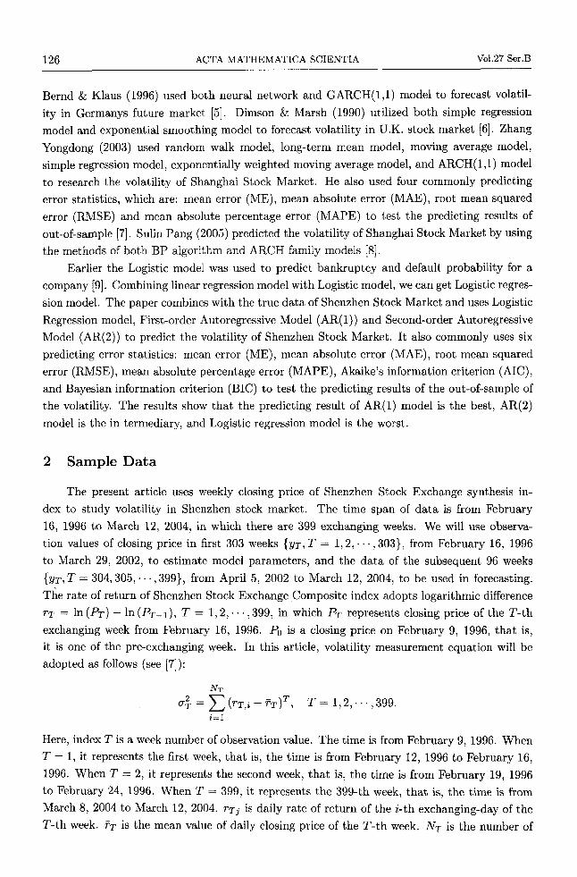
Bernd & Klaus (1996) used both neural network and GARCH(1,l) model to forecast volatility in Germanys future market [5]. Dimson & Marsh (1990) utilized both simple regression model and exponential smoothing model to forecast volatility in U.K. stock market [6]. Zhang Yongdong (2003) used random walk model, long-term mean model, moving average model, simple regression model, exponentially weighted moving average model, and ARCH( 1,l) model to research the volatility of Shanghai Stock Market. He also used four commonly predicting error statistics, which are: mean error (ME), mean absolute error (MAE), root mean squared error (RMSE) and mean absolute percentage error (MAPE) to test the predicting results of out-of-sample 171. Sulin Pang (2005) predicted the volatility of Shanghai Stock Market by using the methods of both BP algorithm and ARCH family models [8].

Earlier the Logistic model was used to predict bankruptcy and default probability for a company [9]. Combining linear regression model with Logistic model, we can get Logistic regression model. The paper combines with the true data of Shenzhen Stock Market and uses Logistic Regression model, First-order Autoregressive Model (AR( 1)) and Second-order Autoregressive Model (AR(2)) to predict the volatility of Shenzhen Stock Market. It also commonly uses six predicting error statistics: mean error (ME), mean absolute error (MAE), root mean squared error (RMSE), mean absolute percentage error (MAPE), Akaike’s information criterion (AIC), and Bayesian information criterion (BIC) to test the predicting results of the out-of-sample of the volatility. The results show that the predicting result of AR(1) model is the best, AR(2) model is the in termediary, and Logistic regression model is the worst.

2 Sample Data

The present article uses weekly closing price of Shenzhen Stock Exchange synthesis index to study volatility in Shenzhen stock market. The time span of data is from February 16, 1996 to March 12, 2004, in which there are 399 exchanging weeks. We will use observation values of closing price in first 303 weeks { Y T , T = 1 , 2 , . . . , 303}, from February 16, 1996 to March 29, 2002, to estimate model parameters, and the data of the subsequent 96 weeks { Y T , T = 304,305,. . . , 399}, from April 5, 2002 to March 12, 2004, to be used in forecasting. The rate of return of Shenzhen Stock Exchange Composite index adopts logarithmic difference TT = In (PT) - In ( P T - ~ ) , T = 1,2, . . . , 399, in which PT represents closing price of the T-th exchanging week from February 16, 1996. Po is a closing price on February 9, 1996, that is, it is one of the pre-exchanging adopted as follows (see [7]):

week. In this article, volatility measurement equation will be

N r

i=l

Here, index T is a week number of observation value. The time is from February 9, 1996. When T = 1, it represents the first week, that is, the time is from February 12, 1996 to February 16, 1996. When T = 2, it represents the second week, that is, the time is from February 19, 1996 to February 24, 1996. When T = 399, it represents the 399-th week, that is, the time is from March 8, 2004 to March 12, 2004. rTj is daily rate of return of the i-th exchanging-day of the T-th week. FT is the mean value of daily closing price of the T-th week. NT is the number of

No. 1 Pang et al: COMPARISON OF FORECASTING MODELS OF VOLATILITY 127

days of exchange during the T-th weeks. Fig.1 shows the observation values of weekly closing price of Shenzhen Stock Exchange

synthesis index, from February 16, 1996 to March 12, 2004. In the researching sample region, the closing price of Shenzhen Stock Exchange synthesis index exists in evident volatility. But it presents rising stream evidently in this region.

Fig.2 shows the observation values of weekly rate of return. Fig.3 shows the observation values of weekly volatility. In the researching sample region, the volatility on the 43-rd week (5" = 43, that is, the time is from December 16, 1996 to December 20, 1996) of Shenzhen Stock Exchange synthesis index is the largest. 043 = 0.146066.

700

600

500 0 .- ZL 2 400

0

.- m 0 -

300

200

100 0 50 100 150 200 250 300 350 400

T Fig.1 Raw data of weekly closing price

0 16

0.14

0 12

0.1 z - { O 08 - $ 0 06

0.04

0.02

0 0 50 100 150 200 250 300 350 400 0 50 100 150 200 250 300 350 400

T T

Fig.:! Raw data of weekly rate of return Fig.3 Raw data of weekly volatility

3 Logistic Predicting Model

In this article, we use logistic regression model to predict historical observation values about weekly closing price in order to predict the next term closing price. Logistic predicting model

ACTA MATHEMATICA SCIENTIA Vo1.27 Ser.B 128

has three characteristics: monotone increasing, increasing finiteness, and shape. The model 'uses historical observation values of saturation increasing variable to evaluate three unknown variable parameters presented in this model.

Assume that the unknown time-variable parametes: KT, PT, TT have the character of saturation increasing. y1, y2, . . . , YT are observation values of a stochastic process. Then the Logistic predicting model with time-variable parameter is expressed by:

in which, T(T = I, 2 , . . . ,303) is the period number of historical data, L is the term number of predicting. We change the model into the following equivalent form:

- = BT + ATeCrTL, YT+L

1

where ePT

kT kT , AT=- . BT = -

1

To time sequence I, I,. . . , -L which consists of reciprocals of the observation values ~i Ya YT

y1, y2,. . . , YT, the average of the first-order exponential smooth of equation (2) is:

in which, a(0 < a < 1) is a smooth constant. We choose a = 0.5 by comparison here. When i = 0 and T = 0, we have S,$') = a/yo. yo is the opening price of the first week.

The average of the second-order exponential smooth of equation (2) is:

a 2 ( 1 - a)i(i + 1) T $1 = c

YT-i i=O

If i = 0 and T = 0, we have s p = a2/yo.

The average of the third-order exponential smooth of equation (2) is:

(4)

If a = 0 and T = 0, we have $1 = a3/yo.

Equation (3) can be further written by:

Using t'he same condition, (4) and (5) can also be further written as:


On the other hand, l / y ~ - i (i = 1 , 2 , . . . ,T ) is substituted for equation (2). We can get three evaluating values 3$), SF’, Sg’ of the average of exponential smooth of the T-th period. That is, we can get three equations as follows:

On the left hand sides of the above equations, the three averages of exponential smooth

Equation (9), (lo), (11) can be further written as follows: can be calculated by the time sequence which are reciprocals of the past observation values.

414) A ~ e - ~ ~ a ~ 3 A ~ e - ~ ~ a ~ ( 1 - a ) - 0) (e-rT - + 1) s$’ X BT + + + e-TT + a - 1 2 (e-TT + a - 1)2 2 (e-TT + a - q3

The solutions of the equation groups are just evaluating values of the unknown parameter variables BT, AT, T-T of the T-th period. They can be expressed as follows:

Therefore, the evaluating values of the time-variable parameters KT and ,& of the T-th period in the Logistic predicting model (See equa. (1)) can be expressed as follows:

I - I @T = In AT - In&.

The predicting values of the time-variable parameters KT and ,& of the 304-th period, the 305-th periods, . . ., the 399-th period are listed in Table 1.

130 ACTA MATHEMATICA SCIENTIA Vo1.27 Ser.B

336 458.2799 337 363.72001 338 368.78089 339 385.8532

week

-23.3936 0.52572 384 358.4011 -28.4915 0.311922 -26.6145 0.108889 385 365.56556 -27.5828 1.27973 -26.9011 0.119664 386 366.48452 -24.6415 0.722432 -27.2161 0.185506 387 363.33082 -26.0693 0.525175

Tat

348 349 350 351

tle 1 Predicting values of the time-variable parameters &, &, ?T of Logistic ma T I KT I PT I '?T I T I KT I PT I =vT

304 I 482.05105 I -27.5357 I 0.270066 I 352 I 423.64964 I -27.6546 I 3.195247

427.76286 -28.5653 0.351156 396 355.53881 -24.6321 0.169255 441.92558 -28.8328 0.161054 397 474.12965 -25.7454 0.182952 426.76937 -31.753 0.509015 398 446.76654 -27.0102 0.340302 423.69584 -24.465 3.77973 399 444.78055 -28.2904 0.37562

del

324 I 489.86334 1 -27.5137 I 2.558668 I 372 I 433.95833 I -29.1974 I 0.088722

328 I 492.52797 I -27.2813 [ 0.503577 I 376 I 410.26813 I -27.3236 I 0.190329 329 I 495.54313 I -26.768 I 0.346218 I 377 I 455.43011 I -28.3749 I 0.063015

340 I 406.13152 I -35.459 I 0.663477 I 388 I 374.37948 I -34.2678 I 0.624981 I

341 I 285.14054 I -31.4487 1 0.016176 I 389 I 363.93758 I -28.5524 I 0.213899

ecoces again.

No.1 Pang et al: COMPARISON OF FORECASTING MODELS OF VOLATILITY 131

We can use the logistic predicting model (1) to predict the closing price of the next 96 weeks (from April 5, 2002 to March 12, 2004, T = 304,305, ,399 ) by substituting the evaluating values of KT and ,& into model (1). Fig.4 is a comparison between the observation values of the closing price and the predicting values of the closing price, in which the solid line is the observation values of the closing price and the dashed line is the predicting values of the closing price. Fig.5 is a comparison between the observation values of the volatility and the predicting values of the volatility, in which the solid line is the observation values of the volatility and the dashed line is the predicting values of the volatility.

800 I 0.35 r

i 700

I -Rawdata 1 .... Logist forecting

1 II 11 I /

0 600- .-

4 0 0 -

300 -

200 0 10 20 30 40 50 60 70 80 90 100

T Fig.4 Observation values and predicting values of logistic to weekly closing price

0 10 20 30 40 50 60 70 80 90 100 T

Fig.5 Observation values and predicting values of logistic to weekly volatility

We can see from Figures 4 and 5 that there are a few predicting results are correct, however, there are also some predicting results that produce serious deviation when we use logistic model to carry out prediction. At the same time, the phenomenon also explains that the development in Chinese Stock Market is incomplete. The atmosphere of gambling is very strong in the stock market, thus it leads to invalidation of the predicting results of the model to certain degree.

4 Predicting Model of Both AR(1) and AR(2)

It is assumed that x 1 , x 2 , . . . , X T are realizations of a stochastic process. The First-order Autoregressive Process (called AR( 1) model) of x t (1 5 t 5 2') can be expressed by

The Second-order Autoregressive Process (called AR(2) model) of x t ( 1 5 t 5 2') can be expressed as

Where, E t - M N ( 0 , u2) is a white-noise process.

Autocovariance of xt is defined by Y k = $ T

t=k+l Xtxt-k, k = 0, k1, If2, -.

ACTA MATHEMATICA SCIENTIA Vo1.27 Ser.B 132

Autocorrelation Function (ACF) of xt is defined by

cov(xt, XGt-k) - - 3. p k = d m ) ' COV(xt-k, X t - k ) 70

When predicting the volatility in Shenzhen Stock Market, we choose time-lag k = 40. By zero-mean processing for the observation values of both the weekly closing price and the volatility, we can get two zero-mean series which are {Wt} and {&}(t = 1,2, . . . ,264), respectively. Their ACF P k and PACF $kk are listed below in Table 2. Note that it only lists the values for k = 1 , 2 , * . . , 1 8

Table 2 The values of both ACF and PACF (k = 1,2, . . . ,18)

9 I 0.622 I 0.014 I 0.030 I -0.004 I 18 I 0.378 I 0.083 I -0.107 1 0.096

Fig.6 and Fig.7 are autocorrelation function figure and partial autocorrelation function figure, respectively for the zero-mean series {Wt} of the weekly closing price.

I O C - Coefficient 1

-0.5 t - 1 0 1

1 3 5 7 9 1 1 1 5 19 23 27 31 35 39 13 17 21 25 29 33 37

Lag Number

10

0.5

9 < o z *

-0.5

-10

1 3 5 7 911 15 19 23 27 31 35 39

Lag Number 13 17 21 25 29 33 37

Fig.6 Autocorrelation function figure of the Fig.7 Partial autocorrelation function figure of the observation values of weekly closing price observation values of weekly closing price

We know from Fig.6, the autocorrelation function f i k of the zero-mean series {Wt} of weekly closing price is attenuating when k is increasing. Thus we can think it is drag-trail. And the partial autocorrelation function &k waves near zero when k > 1 . Thus we can think it is cut-trail. Therefore, the zero-mean series { Wt } of weekly closing price of Shenzhen Integrated Index is a stationary autoregressive process.

No.1 Pang et al: COMPARISON OF FORECASTING MODELS OF VOLATILITY 133

(1) The series { Wt} should be a stationary AR(1) process. The model can be expressed by

and the AR( 1) model of { vt } can be expressed by

vt = 0.16vt-l + Et. (18)

- 0.061546 , while k > 2, all $kk I ^ I (2) But when k > 1 , because = 0.107 > & - , (k = 1,2, -. ,18) are not larger than

for a stationary AR(2) process. The model can be assumed by = 0.123091 , therefore, the series {Wt} is also taken

where, the parameters $1 and 4 2 can be evaluated by the binary linear equations given below:

$1 + 0.95542 = 0.955, { 0.95541 + 4 2 = 0.906.

We solve it and get $1 = 1.020404, $2 = -0.06849. Thus the AR(2) model of {Wt} can be expressed by

Applying the same method, the AR(2) model of the zero-mean series of the volatility can be assumed by

vt = Cp1vt-1+ (pzvt-2 + E t ,

where, the parameters $1 and $2 can be evaluated by the binary linear equations given below:

{ 0.16F1 + dz = 0.024.

= 0.220033. Thus the AR(2) model of {vt} can be

$1 + 0.16& = 0.16,

We solve it and get (PI = 0.124795, expressed as

According to equations (17) and (19), reverting to the zero-mean series {Wt} , we use the models of both AR(1) and AR(2) to predict the next 96 weeks (from April 5, 2003 to March 12, 2004) of weekly closing price. The predicting results of the model of both AR(1) and AR(2) are illustrated in Fig.8 and Fig.9, respectively. On the other hand, according to equations (18) and (20), reverting to zero-mean series {K}, we use the models of both AR(1) and AR(2) to predict the next 96 weeks (from April 5, 2003 to March 12, 2004) of the volatility. The predicting results of the model of both AR(1) and AR(2) are illustrated in Fig.10 and Fig.11, respectively. In Fig.8, 9, 10, and 11, the dashed line is the predicting results and the solid line is the observation values.


400

- Raw data 380 1 360 .... AR(1) forecting

" ."

360 - .... AR(2) forecting

3401 ' I I ' I ' ' ' ' I 340' ' ' ' ' ' ' ' ' ' 0 10 20 30 40 50 60 70 80 90 100 0 10 20 30 40 50 60 70 80 90 100

T Fig.8 Observation values and predicting

values of AR(1) to weekly closing price

0.051- - Raw data .._. AR(1) forecting

-0.Oll ' ' ' ' ' ' ' ' '

T Fig.9 Observation values and predicting

values of AR(2) to weekly closing price

- Raw data ...- AR(2) forecting 0.04

0.03 x - .- c 'S 0.02 9 -

0.01

0

0 10 20 30 40 50 60 70 80 90 100 0 10 20 30 40 50 60 70 80 90 100 T T

Fig.10 Observation values and the predicting Fig.11 bservation values and the predicting

values of AR(1) to weekly volatility

By observing Fig.8 and Fig.9, we discover that the predicting results of the models of both AR(1) and AR(2) to the weekly closing price of Shenzhen Integrated Index are not evidently different. And the predicting results to their volatility are not evidently different either (See Fig.10 and Fig.11). However, compare Fig.8 and 11 with Fig.4 and 5 , whether forecasting weekly closing price or forecasting the volatility, the predicting results of both AR(1) and AR(2) all are evidently better than Logistic regression models.

values of AR(2) to weekly volatility

5 Test to Forecasting Error

In this section, we will further illuminate the predicting ability to the three models which are AR(l), AR(2), and logistic regression model by error testing to out-of-sample of the volatility.

Forecasting error implies a deviation between the predicting results and the practical results. Generally, forecasting error always exists whichever predicting model is adopted. For


Sort MAPE

Sort

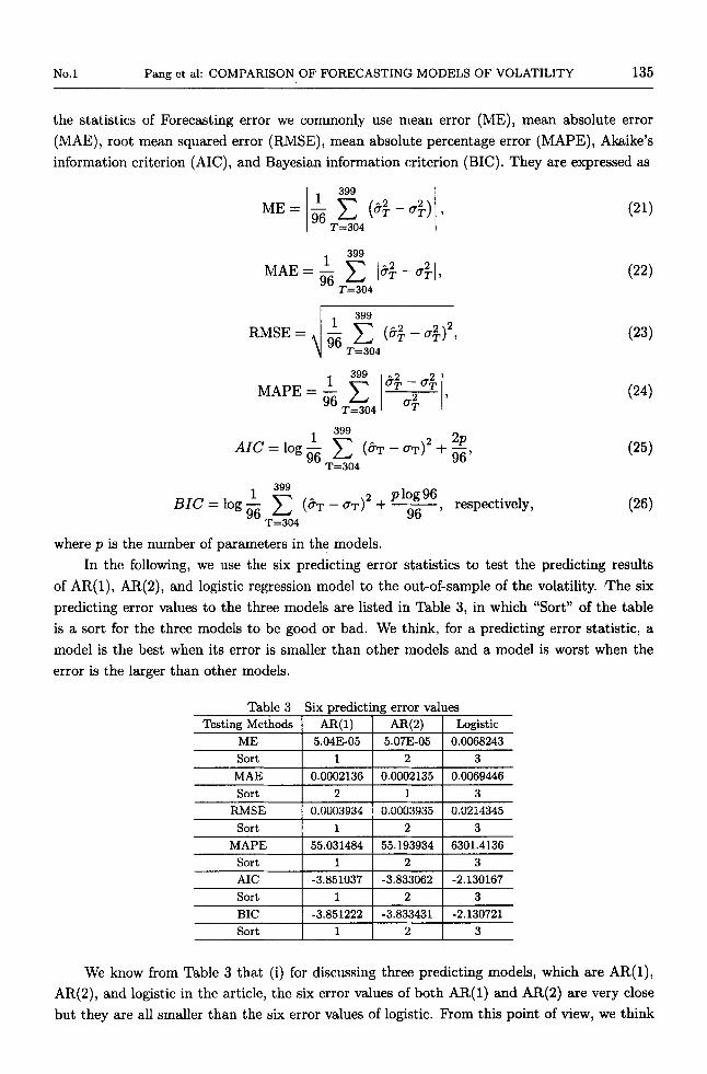
the statistics of Forecasting error we commonly use mean error (ME), mean absolute error (MAE), root mean squared error (RMSE), mean absolute percentage error (MAPE), Akaike’s information criterion (AIC), and Bayesian information criterion (BIC). They are expressed as

1 2 3 55.031484 55.193934 6301.4136

1 2 3

399

M E = - C (6$-&)1, T=304

399

1 9’6 1

96 MAE= - C I&$ -.$I,

T=304

Sort 1

399 ~ ~ ~ = i o g - 1 c ( c T - ~ T ) 2 +

96 T=304

2 I 3

399 1 2 plog96

96 ’ 96 BIG’= log- C ( 6 ~ - CT) + ___

T=304

respectively

where p is the number of parameters in the models. In the following, we use the six predicting error statistics to test the predicting results

of AR(l) , AR(2), and logistic regression model to the out-of-sample of the volatility. The six predicting error values to the three models are listed in Table 3, in which “Sort” of the table is a sort for the three models to be good or bad. We think, for a predicting error statistic, a model is the best when its error is smaller than other models and a model is worst when the error is the larger than other models.

Table 3 Six predicting error values

MAE Sort 1 2 1 1 1 3

RMSE 1 0.0003934 1 0.0003935 1 0.0214345

AIC I -3.851037 I -3.833062 I -2.130167 Sort 1 1 1 2 1 3

We know from Table 3 that (i) for discussing three predicting models, which are AR(l), AR(2), and logistic in the article, the six error values of both AR(1) and AR(2) are very close but they are all smaller than the six error values of logistic. From this point of view, we think


the predicting results of both AR(1) and AR(2) are all better than Logistic’s. (ii) compare the six predicting error values of both AR(1) and AR(2), although the six error values of both AR(1) and AR(2) are very close, but except MAE, all AR(1) are better than AR(2). (iii) we can make conclusion that, to the predicting results, AR(1) is the best, AR(2) is the intermediate, and logistic regression model is the worst.

6 Conclusions

This article has adopted the closing price of every weekend in Shenzhen Integrated Index to research the volatility in Shenzhen Stock Market based on the three models which are logistic, AR(l), and AR(2). The time span of data is from February 16, 1996 to March 12, 2004, which is 399 exchanging weeks. We use observation values of the closing price in first 303 weeks {YT, T = 1,2, . . . ,303) from February 16, 1996 to March 29, 2002, to estimate model parameters, and the data of the next 96 weeks { y ~ , T = 304,305,. . . ,399}, from April 5 , 2002 to March 12, 2004, for forecasting. By introducing both methods of index smoothing method and timevariable parameter estimation, the time-variable parameters of logistic regression model are estimated. And according to the analysis results of, zero-mean series of the weekly closing price, both AR(1) model and AR(2) model of zero-mean series of the weekly closing price and its zero-mean series of volatility rate are set up, respectively. And then the paper adopts six sorts of common statistical methods of predicting error which are mean error (ME), mean absolute error (MAE), root mean squared error (RMSE), mean absolute percentage error (MAPE), Akaike’s information criterion (AIC), and Bayesian information criterion (BIC) to test the predicting results of the out-of-sample. The results show that the predicting result of AR(1) model is the best, AR(2) model is intermediate, and logistic regression model is the worst.

References

1 Engle R F. Autoregressive conditional heteroskedasticity with estimates of the variance of U. K. inflation.

2 Bollerslev T. Generalized autoregressive conditional heteroskedasticity. Journal of Economitrics, 1986, 31:

3 Bollerslev T, Chou R T, Kroner K F. ARCH modeling in finance. Journal of Economitrics, 1992, 52: 1-59 4 Akgiray V. Conditional heteroskedasticity in time series of stock returns: Evidence and forecasts. Journal

of Business, 1989, 62: 55-80 5 Bernd F, Klaus R. Volatility estimation with neural network. Proceedings of the IEEE/IAFE Conference

on Computational Intelligence for Financial Engineering. Mar 24-26 1996, New York, USA, 1996. 177-181 6 Dimson E, Arsh M P. Volatility forecasting without data-snooping. Journal of Banking and Finance, 1990, 14: 399-421

7 Zhang Y D. Volatility forecasting m.odels in the Shanghai stock market: A comparison. Journal of Man- agement Engineering, 2003, 3

8 Pang S. Credit scoring models and the predicting models in stock market approach of statistics. In: Neural Network and Support Vector Machine. Beijing: Science Press, 2005

9 Martin D. Early warning of bank failure: a logit regression approach. Journal of Banking and Finance,

Economitrica, 1982, 50: 987-1008

307-327

1977. 249-276

a comparison of forecasting models of the volatility in shenzhen stock market

Documents