a comparative analysis of machine learning methods for classification type decision problems in...

RESEARCH Open Access

A comparative analysis of machine learningmethods for classification type decisionproblems in healthcareNahit Emanet1, Halil R Öz2, Nazan Bayram3 and Dursun Delen4*

* Correspondence: [email protected] of ManagementScience and Information Systems,Spears School of Business,Oklahoma State University,Stillwater, OK, USAFull list of author information isavailable at the end of the article

Abstract

Advanced analytical techniques are gaining popularity in addressing complexclassification type decision problems in many fields including healthcare andmedicine. In this exemplary study, using digitized signal data, we developedpredictive models employing three machine learning methods to diagnose anasthma patient based solely on the sounds acquired from the chest of the patient ina clinical laboratory. Although, the performances varied slightly, ensemble models(i.e., Random Forest and AdaBoost combined with Random Forest) achieved about90% accuracy on predicting asthma patients, compared to artificial neural networksmodels that achieved about 80% predictive accuracy. Our results show that non-invasive, computerized lung sound analysis that rely on low-cost microphones andan embedded real-time microprocessor system would help physicians to make fasterand better diagnostic decisions, especially in situations where x-ray and CT-scans arenot reachable or not available. This study is a testament to the improving capabilitiesof analytic techniques in support of better decision making, especially in situationsconstraint by limited resources.

Keywords: Classification; Data mining; Machine learning; Decision making; Asthma;Pulmonary sound signals; Discrete wavelet transformation

BackgroundAs the decision situations become increasingly more complex, advanced analytical

techniques are gaining popularity in addressing wide variety of problem types (descrip-

tive, predictive and prescriptive) in many fields including healthcare and medicine

(Delen et al. 2009). Because of the rapid increase in the collection and storage of large

quantities of data (facilitated by improving software and hardware capabilities coupled

with increasingly lower cost of acquiring and using them), data and model driven deci-

sion making (a.k.a. analytics) is becoming a mainstream practice in every field imagin-

able (from art to business, medicine to science). One area where faster and better

decisions could make a significant difference is in healthcare/medicine. This data rich

field can undoubtedly use what modern day decision analytics has to offer (Oztekin

et al. 2009). In this study, we used analytics to address a classification type decision

problem, namely prediction of asthma using only the chest sound signals obtained

from actual patients using ordinary microphones.

© 2014 Emanet et al.; licensee Springer. This is an open access article distributed under the terms of the Creative CommonsAttribution License (http://creativecommons.org/licenses/by/2.0), which permits unrestricted use, distribution, and reproduction in anymedium, provided the original work is properly cited.

Emanet et al. Decision Analytics 2014, 1:6http://www.decisionanalyticsjournal.com/1/1/6

mailto:[email protected]

mailto:[email protected]

http://creativecommons.org/licenses/by/2.0

Auscultation of pulmonary sounds provides invaluable clinical information on the

health of the respiratory system. It is known in medicine that sounds emanating from

the respiratory system are correlated with the underlying pulmonary pathology. The

changes in lung structure change the spectrum of sounds heard over the chest wall. In

addition to the typical sounds associated with the breathing process, extra or additional

sounds are heard over the normal pulmonary sounds. These additional sounds are

called adventitious pulmonary sounds and detection of these adventitious sounds is an

important part of the respiratory examination that allows the physician to detect some

pathological diseases.

Adventitious pulmonary sounds can be divided into five categories: wheezes, crackles,

stridors, squawks and rhonchi. Although stethoscope is widely used by physicians as a

simple, non-invasive tool for the auscultation of pulmonary sounds, it has been

regarded as a tool with low diagnostic value, not only because pulmonary sounds for

each patient are significantly different and they change for the same patient over time,

but also because it is a subjective process that depends on the experience and hearing

capability of physician. Stethoscope is not an ideal acoustic instrument either; it attenu-

ates frequency components of pulmonary sounds above 120 Hz by making it impossible

for the physician to hear pathological sounds of higher frequencies. Moreover, ausculta-

tion with stethoscope does not allow long term monitoring of pulmonary sounds.

Electronic auscultation of pulmonary sounds (Earis and Cheetham 2000), on the

other hand, is a reliable and quantitative method that eliminates the shortcomings of

stethoscope. In this system, a microphone placed at designated locations on the chest

of a patient provides non-stationary pulmonary sound signals which can be recorded

for an extensive period of time for subsequent analysis. Significant diagnostic informa-

tion can be obtained from the frequency distribution of these signals.

The ultimate goal of this work is to develop a fully automated, highly accurate, low-

cost and easy to use diagnostic tool for pulmonary diseases as a decision support tool

for a physician. However, in this paper, we initially restrict our efforts on studying and

diagnosing asthma, because of the prevalence of asthma in the world as one of the

highest among all pulmonary disorders. It is estimated that 300 Million people world-

wide suffers from asthma (Masoli et al. 2010) and by 2025, the number of patients ex-

pected to exceed 100 Million. The symptoms of asthma include wheezing, shortness of

breath, chest tightness and cough. Wheezes are characterized by periodic waveforms

with a dominant frequency greater than 100 Hz, and lasting for longer than 150 ms

(Oz et al. 2010). Multiple monophonic wheezes occurring simultaneously in a patient is

known as a classic symptom for asthma disease (Ali et al. 2009).

In the literature, a large number of studies have focused on classifying pulmonary dis-

eases. Doyle (1994) tried to classify adventitious pulmonary sounds (crackles, wheezes,

pleural-friction rub and stridor) using artificial neural network with a reported accuracy

of 83%. Sankur et al. (1994) build classification models to differentiate between normal

and adventitious pulmonary sounds using auto-regression models, and achieved a pre-

diction accuracy of 87%. Gavriely (1995) tested and demonstrated the effectiveness of

computerized pulmonary sound analysis in addition to existing spirometry pulmonary

function test. Pesu et al. (1998) used a wavelet packet-based method for the detection

of adventitious pulmonary sounds, and learning vector quantization (LVQ) for the clas-

sification with limited success on classification accuracy. Kandaswamy et al. (2004)

Emanet et al. Decision Analytics 2014, 1:6 of 20http://www.decisionanalyticsjournal.com/1/1/6

applied wavelet transform for the time-frequency analysis of pulmonary sound signals;

used variety of artificial neural networks architectures for the classification; and

achieved classification accuracy as high as 94%. Murphy et al. (2004) focused on pneu-

monia and included a customized pneumonia score to features obtained from sound

analysis, and time expanded waveform analysis is employed for automated classifica-

tion. Similarly, after two years later, Kahya et al. (2006) also included customized pa-

rameters such as crackles parameters based on the duration of crackles during a breath

cycle, and employed k-nearest neighbor algorithm for automatic classification, and ar-

chiving acceptable prediction accuracy. Ono et al. (2009) focused on interstitial pneu-

monia (IP) and investigated inspiratory lung sounds with Fast Fourier transformation

to convert the data into a machine usable digitized format. Mohammed (2009), in order

to classify pulmonary sounds, used cepstral analysis and Gaussian mixture models and

achieved prediction accuracy close to 90%. Oz et al. (2009) combined Fast Fourier

transformation with genetics programming (GP) and Fuzzy C-Means clustering to

analyze pulmonary diseases. They also achieved prediction accuracy close to 90%.

Many of the above mentioned studies employed feature extraction techniques based on

wavelet transformation, Fast Fourier transformation, Mel-frequency cepstral coefficients.

For the automatic classification they employed artificial neural networks, Gaussian mix-

ture models, learning vector quantization, genetics programming, k-nearest neighbor,

among others.

In this study, we used a four-stage process to analyzed pulmonary sound signals:

normalization, wavelet decomposition, feature extraction, and the classification (where

we classified respiratory sounds using Random Forest algorithm, AdaBoost combined

with Random Forest and artificial neural networks). Pulmonary sounds recorded from

various subjects are normalized so that they would have approximately the same loud-

ness level irrespective of the subject and/or environmental conditions. After norma-

lization, feature vectors are formed by using this normalized data. The signals are

decomposed into frequency sub-bands using discrete wavelet transformation (DWT)

(Mallat 2009, Jensen and Harbo 2001 and Daubechies 1990. A set of statistical features

is extracted from these sub-bands to represent the distribution of wavelet coefficients.

These statistical feature vectors then introduced to the classification algorithms to

evaluate the pulmonary sound signals as either normal or asthma. Block diagram of the

diagnostic system is depicted in Figure 1.

MethodsSystem description and data collection

All pulmonary sounds were recorded at University of Gaziantep, Faculty of Medicine.

In particular, recording of respiratory sounds was conducted in a clinical laboratory.

Respiratory acoustic signals were recorded using Sony ECM-T150 electret condenser

microphones with air coupler applied over right and left posterior bases of the lungs:

positions P4 and P5, respectively. These air coupled microphones had linear frequency

response between 50 Hz and 15 KHz. They were attached to the body of the subjects

at the aforementioned positions.

Amplification and band pass filtering (Kester 2005) was performed prior to analogue-

to-digital conversion with a 16-bit resolution at a sampling rate of 8K samples/s per

channel in order to remove environmental sounds, heart and muscle sounds, and


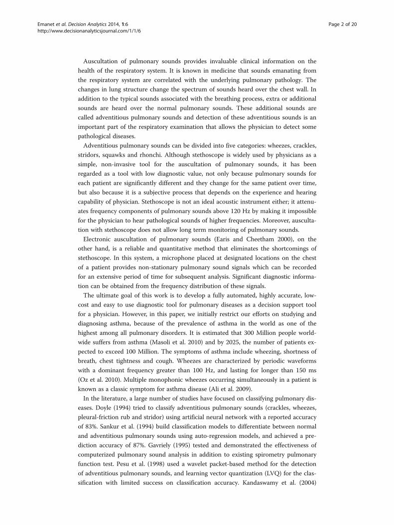
friction sounds caused by the movements of microphones. SSM2019, OP275 and

MAX295 integrated circuits are used in the amplification and band pass filtering circuit

as shown in Figure 2. SSM2019 is a very low noise microphone preamplifier, which is

often used to amplify microphone’s low output voltage, typically in the 0 to 100 micro-

volt range, to a level that is usable for recording. The gain of the preamplifier was set

to 11 by 1 KΩ metal film resistor to obtain minimum total harmonic distortion. The

filtering stage comprises both an active high pass Bessel filter of order six and an active

low pass Butterworth filter of order eight. While Butterworth filter was optimized for

maximal gain flatness, Bessel filters provided low overshoot and fast settling. High pass

filter with cut-off frequency of 100 Hz was realized by three Analog Devices OP275 op-

erational amplifiers. High pass filter was followed by a low pass filter with cut-off fre-

quency of 2 KHz. It was implemented by using MAX295 8th-Order Switched-

Capacitor Filter.

After pulmonary sound signals are acquired from right and left posterior bases of the

lungs, they are digitized and digitally filtered for further noise removal. Since inspir-

ation and expiration phases have different information, the signals are divided into

those parts separately.

Figure 1 A high-level conceptual diagram of the diagnostic process.


Ten healthy and ten asthmatic patients were studied during the data collection

phase. The specifics about those twenty subjects are shown in Table 1. All record-

ings were performed under the supervision of a senior physician who was specialized

in pulmonary diseases using an ARM based mobile biomedical data acquisition

device (Fuber 2000 and Catmakas et al. 2009). The number of sound recordings

from the 20 subjects was 40 in total. The ages of the subjects were in the range of 16

to 62. There were 6 smokers and 14 nonsmokers. Seven subjects were male and 13

were female.

Though listed in Table 1, in the formulation of this study, only the sound signals are

used as independent variables; none other special condition (e.g., socio-demographic

characteristics) like age, sex, weight, and smoking habits were taken into consideration.

Percentage of forced vital capacity (FVC) and forced expiratory volume in one

second (FEV1) values, which are used in pulmonary function test (PFT), are also

shown in Table 1. During clinical evaluation, subjects were asked to inhale as

deeply as possible up to their total lung capacity and then exhale completely as fast

as and as hard as possible. The volume change of the lung during exhalation is

called as FVC. The FEV1 is also defined as the volume exhaled during the first

second of FVC.

Asthma is a common disease characterized by inflammation and hyper-reactivity in

the airways which causes reversible airflow limitation. Patients with well controlled

asthma demonstrate normal breath sounds and lung function whereas in poorly con-

trolled asthma or during exacerbations, wheezing is usually heard in parallel with a fall

in FEV1 and FEV1/FVC.

The ratio of FEV1 to FVC is critical in defining lung diseases characterized by airflow

limitation such as asthma, chronic obstructive lung disease, obliterative bronchiolitis,

Figure 2 Block diagram of the diagnostic system.


and cystic fibrosis. In general, FEV1/FVC ratio less than 70% is indicative of airflow

limitation but this level is higher for younger individuals and decreases with age. In the

instances where lung volumes are diminished but the FEV1/FVC ratio is preserved, re-

strictive lung pathology such as interstitial lung disease, pleural effusion or chest wall

deformities may be suspected.

Figures 3, 4, 5, 6 represent pulmonary sound signal waveforms recorded from both

healthy and asthmatic subjects during the inspiration and expiration cycles.

Feature extraction

A critical phase in any prediction model development effort is the characterization and

transformation of the original data (sound signals, in this case) into a form that is most

appropriate to the machine learning models being used. In this study, original pulmon-

ary sound signal vectors were formed by discrete sample points. Mathematical transfor-

mations are applied to these signals in order to obtain further information that is not

readily available in the original raw signal. Some of the most widely used transform-

ation methods include linear transformations, such as principle component analysis

(PCA) and linear discriminant analysis (LDA) (Martinez and Kak 2001 and Breiman

2001). Although PCA and LDA were very commonly used in sound signal transform-

ation operations, they are not necessarily the best ones. In fact, for non-stationary sig-

nals, a wavelet-based time-frequency representation may be used for feature extraction.

The basic idea of the discrete wavelet transform is to represent any arbitrary function f

as a superposition of wavelets. Any such superposition decomposes f into different

Table 1 Clinical values about the subjects

Age Gender Smoke FEV1% FVC% Diagnosis

49 F No 38 84 Asthma

62 F Yes 108 113 Asthma

48 M Yes 32 79 Asthma

60 F No - - Asthma






16 M No 99 106 Asthma

48 F No - - Normal

41 M No 96 98 Normal

18 F No 105 102 Normal


29 F Yes 88 106 Normal


35 M Yes 106 118 Normal





scale levels, where each level is then further decomposed with a resolution adapted to

the level.

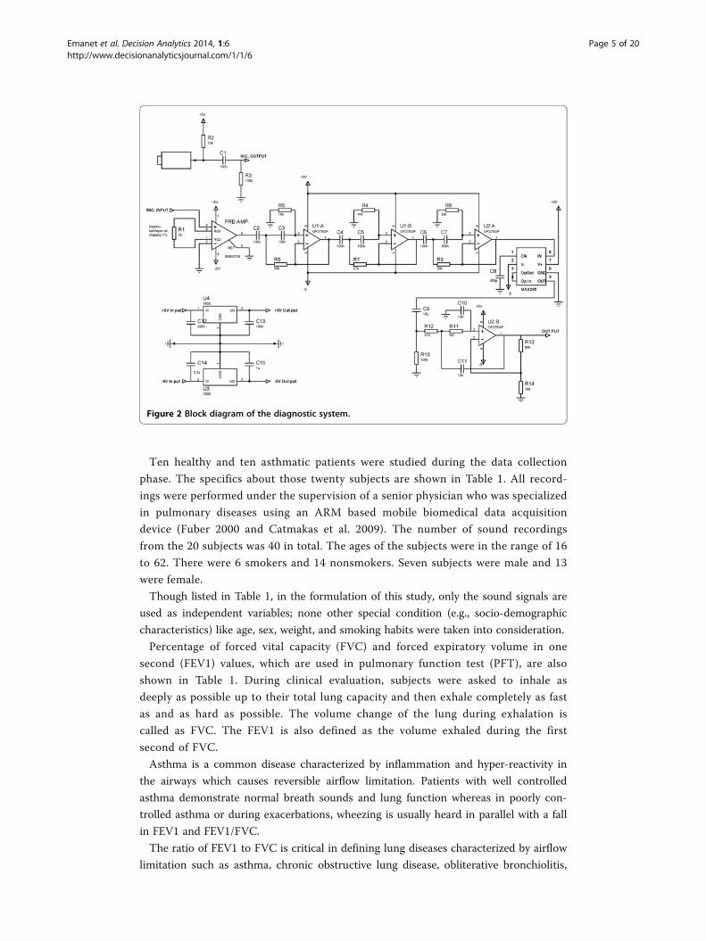
The discrete wavelet transformation of a signal, f[n], is calculated by passing it

through two digital filters and two down-samplers by 2. Digital filters are

low-pass filter, h, and its complementary high-pass filter, g. The down-sampled

outputs of high-pass and low-pass filters provide the detail signal, D, and the

approximation signal, A, respectively as depicted in Figure 7. While this trans-

form reduces the time resolution of the output signal by half, it doubles its

frequency resolution.

This decomposition was recursively repeated to further increase the frequency reso-

lution. At each level, approximation coefficients was decomposed with high and low

pass filters and then down-sampled. The procedure of 3-level decomposition of a signal

f[n] is represented as a binary tree as depicted in Figure 8. In order to perform wavelet

Figure 3 Inspiration cycle after digital filtering for an asthmatic patient.

Figure 4 Expiration cycle after digital filtering for an asthmatic subject.


analysis of pulmonary sounds, Matlab program was used. Daubechies db8 with 6 levels

(Daubechies 1990) was used as the mother wavelet in the analysis.

Selection of the number decomposition levels is very important in the analysis of sig-

nals using DWT. The levels were chosen in such a way that frequency sub-bands of the

decomposed signal correlated well with the frequencies required for the classification.

Since the pulmonary sounds do not have any useful frequency components below 60

Hz and above 2000 Hz, the number of levels was chosen as six by taking into consider-

ation the sampling frequency of 8 KHz. Therefore, the signal was decomposed into the

details D1-D6 and one final approximation A6. Figure 9 depicts the pulmonary signal,

s, recorded from the right posterior base of a healthy subject. The decomposition is

done by using Daubechies db8 wavelet with 6 levels. The ranges of frequency sub-

bands are given in Table 2.

Figure 5 Inspiration cycle after digital filtering for a healthy subject.

Figure 6 Expiration cycle after digital filtering for a healthy subject.


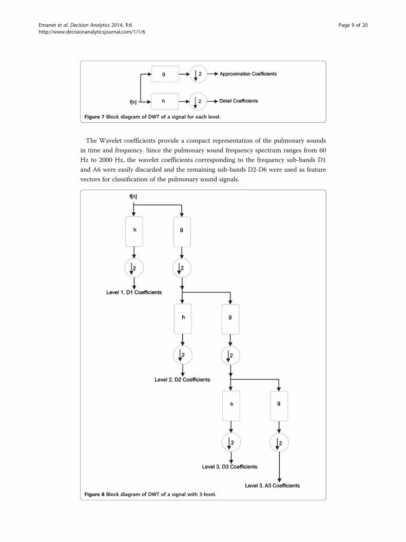
The Wavelet coefficients provide a compact representation of the pulmonary sounds

in time and frequency. Since the pulmonary sound frequency spectrum ranges from 60

Hz to 2000 Hz, the wavelet coefficients corresponding to the frequency sub-bands D1

and A6 were easily discarded and the remaining sub-bands D2-D6 were used as feature

vectors for classification of the pulmonary sound signals.

Figure 7 Block diagram of DWT of a signal for each level.

Figure 8 Block diagram of DWT of a signal with 3-level.


In order to further reduce the size of the feature vectors, the following statistical fea-

tures were used to represent the time-frequency distribution of the pulmonary sound

signals.

1. Mean values of the wavelet coefficients in each sub-band.

2. Average power of the wavelet coefficients in each sub-band.

3. Standard deviation of the wavelet coefficients in each sub-band.

4. Ratio of the absolute mean values of adjacent sub-bands.

Figure 9 Signal decomposition by db8 with 6 levels.

Table 2 Frequency sub-bands in wavelet decomposition

Decomposed signal levels Frequency range (Hz)

D1 2000 – 4000

D2 1000 – 2000

D3 500 – 1000

D4 250 – 500

D5 125 – 250

D6 62.5 – 125

A6 0 – 62.5


Table 3 presents the statistical features of two sample recordings: one from healthy

subject and one from subject with asthma disease.

Classification methods used

Random forest algorithm

Random Forest is essentially an ensemble of unpruned classification trees. It gives ex-

cellent performance on a number of practical problems, largely because it is not sensi-

tive to noise in the data set, and it is not subject to overfitting. It works fast, and

generally exhibits a substantial performance improvement over many other tree-based

algorithms.

The classification trees in the Random Forest are built recursively by using the Gini

node impurity criterion (Raileanu and Stoffel 2004) which is utilized to determine splits

in the predictor variable. A split of a tree node is made on variable in a manner that re-

duces the uncertainty present in the data and hence the probability of misclassification.

Ideal split of a tree node occurs when Gini value is zero. The splitting process con-

tinues until a “forest”, consisting of multiple trees, is created. Classification occurs

when each tree in the forest casts a unit vote for the most popular class. The Random

Forest then chooses the classification having the most votes over all the trees in the for-

est. Pruning is not needed as each classification is produced by a final forest that con-

sists of independently generated trees created through a random subset of the data,

avoiding over fitting. The generalization error rates depend on the strength of the indi-

vidual trees in the forest and the correlation between them. This error rate converges

to a limit as the number of trees in the forest becomes large. Another advantage of

Random Forest is that there is no need for cross validation or a separate test set to get

Table 3 Statistical feature vectors for two classes

Levels Features Normal Asthma

Mean −0.001752 0.001327

D6 Std. Dev. 0.016430 0.224913

Avg. Power 0.000272 0.050483

Mean −0.000198 −0.003998

D5 Std. Dev. 0.029939 0.278092

Avg. Power 0.000895 0.077270

Mean 0.000068 −0.001254

D4 Std. Dev. 0.014396 0.186106

Avg. Power 0.000207 0.034619

Mean 0.000029 −0.000095

D3 Std. Dev. 0.003607 0.072520

Avg. Power 0.000013 0.005258

Mean 0.000009 0.000016

D2 Std. Dev. 0.001441 0.006338

Avg. Power 0.000002 0.000040

mean(abs(D6))/mean(abs(D5)) 8.860058 0.331818





an unbiased estimate of the classification error. Test set accuracy is estimated internally

in Random Forest by running out-of-bag samples. For every tree grown in Random

Forest, about one-third of the cases are out-of-bag (out of the bootstrap sample). The

out-of- bag samples can serve as a test set for the tree grown on the non-out-of- bag

data. The specifics of Random Forest algorithm can be summarized as follows:

1. A number n is specified, which is much smaller than the total number of variables

N (typically ne

ffiffiffiffi

Np

)

2. Each tree of maximum depth is grown without pruning on a bootstrap sample of

the training set

3. At each node, n out of the N variables are selected at random

4. The best split on these n variables is determined by using Gini node impurity

criterion.

Reducing n reduces the strength of the individual trees in the forest and the correl-

ation between them. Increasing it increases both. Using the out-of- bag error rate, an

Figure 10 AdaBoost algorithm.


optimum value of n can be found. This is the only adjustable parameter to which ran-

dom forests is sensitive to. The computational complexity for each tree in Random For-

est is O(Slog(S)ffiffiffiffi

Np

), where S is the number of training cases. Therefore, it can handle

very large number of variables with moderate number of observations.

AdaBoost Algorithm

AdaBoost is a fast, simple and easy to use iterative algorithm which needs only one par-

ameter to tune, i.e. number of iteration, T. It does not subject to over-fitting and easily

identifies outliners which are either misclassified or hard to classify.

AdaBoost algorithm was first introduced by Freund and Schapire (Freund nd Schapire

1997). The algorithm takes a training set consisting of m samples (x1, y1),…,(xm, ym) as in-

put, where each xi belongs to an instance space X, and each label yi belongs to finite label

space Y = {−1, +1} for binary classification. AdaBoost generates a set of weak classifiers,

and linearly combines them in an optimal way into a stronger classifier. The job of a weak

classifier is to find a weak hypothesis ht : X → {−1, +1} using samples drawn from itera-

tively updated distribution, Dt, of the training set. One of the main ideas of the AdaBoost

algorithm is to maintain a weight distribution Dt(i) on training samples xi, (for i=1 .. M),

from which training data subsets St are chosen for each consecutive hypothesis ht. Updat-

ing distribution Dt(i) for every iteration ensures that samples misclassified by the previous

weak classifier are more likely to be included in the training data of the next weak classi-

fier. Error of a weak classifier is measured with respect to distribution Dt as εt ¼ ∑i:ht xið Þ≠yiDt ið Þ. If it is possible for the weak classifier to use weights Dt on the training dataset, then

St becomes Dt. Otherwise, St are constructed by resampling the training data according to

Dt. Adaboost algorithm is depicted in Figure 10. Initially, all weights of the distribution

are set equally, D1(i) = 1/M, so that all samples have equal likelihood to be selected into

the first training dataset, S1. AdaBoost calls a given weak classifier algorithm iteratively in

a series of rounds t = 1 to t = T. A weak hypothesis ht and a training error εt for it are

computed at each iteration, t. The distribution Dt is next updated by αt such that the

Figure 11 A three-layer multi-layer perceptron neural network architecture.


weight of samples misclassified by ht is increased, and the weight of samples correctly

classified by ht is decreased. Thus, AdaBoost concentrates more on difficult samples. αt is

also the weight assigned to weak hypothesis ht so that weak classifiers that have shown

good performance during training phase have more influence at the output than others in

the testing phase.

We employed Random Forest algorithm as a weak classifier in the AdaBoost algorithm

to predict asthma lung sounds. Boosting Random Forest algorithm is somewhat similar to

employing forests of random forests.

Artificial neural networks (ANNs)

We also included Artificial Neural Networks (ANNs) to be compatible or comparable

with the pulmonary disease classification algorithms in the literature (Delen 2009 and

Delen et al. 2010). Over the years, ANNs have found their way into numerous applica-

tions (Haykin 1994) ranging from pattern recognition, prediction to optimization and

control systems. ANNs inspired by biological evidence are designed to solve complex

problems by trying to replicate the networks of the real neurons in the human brain.

ANNs are not intelligent, but they are good at learning underlying patterns and mak-

ing simple rules for complex problems without human intervention.

ANNs can be viewed as weighted directed graphs in which directed edges with

weights are used to connect artificial neuron nodes. ANNs can be categorized as feed-

forward networks and recurrent networks. Properties of feed-forward networks are:

� They are static. i.e. for a given input, they produce only one set of output.

� They are memory-less. i.e. output is independent of the previous network state.

� They have no loops in the directed graph.

On the other hand, because of the feedback loops in the directed graph, recurrent

networks are dynamic systems with memory. The most common form of feed-forward

networks is multi-layer perceptron (MLPNN) which consists of multiple layers of nodes

in a directed graph in which each layer is fully connected to previous and next layer.

Each node in a MLPNN is a computational element that employs a differentiable non-

linear activation function such as sigmoid function to its input. Generally, a MLPNN

consists of input layer, one or more hidden layers and one output layer as shown in

Figure 11.

Table 4 Confusion matrix for the result of random forest classifier

Prediction

Healthy Asthma

Actual Healthy 18 2

Asthma 2 18

Table 5 Confusion matrix for the result of adaboosted random forest classifier

Prediction

Healthy Asthma

Actual Healthy 18 2

Asthma 2 18


In this paper, we used standard MLPNN in which a weight vector w on the arcs A of

network N(w, A) determines a mapping H from the input nodes of N to the output

nodes of N. Learning process in MLPNN can be viewed as iteratively updating the arc

weights w for each input output pair in the training pattern set so that a network can

efficiently perform a specific task. wlij in Figure 11 denotes the weight on the connec-

tion between ith node in layer (l-1) to the jth node in layer l. x is the input vector and y

is the corresponding observed output vector. During the learning process, observed

output y, generated by the network N may not equal to the desired output d. Basic

learning rule in MLPNN is to automatically adjust arc weights w such that a certain

cost function is minimized. The squared-error cost function, E ¼ 12∑

pi¼1∥y

i − di∥ ,

which is the sum of squared differences between the observed and desired outputs for

a set of p training patterns, T = {(x1, d1), (x2, d2), (x3, d3),…, (xp, dp)}, is the most fre-

quently used cost function to minimize total error at the output of the network. There

are several learning algorithms in the literature to train a MLPNN and backpropagation

(BP) algorithm (Rumelhart and McClelland 1986) is the most frequently used one. The

BP algorithm is a gradient-descent method which searches an error surface for points

with minimum error. Optimization methods such as Levenberg-Marquardt (Levenberg

1944 and Marquardt 1963) and quasi-Newton (Broyden 1969) have also been used in

recent years. In all these algorithms, after introducing a new input–output pair to the

network from the training dataset, each weight wlij on arcs of the network is modified

by adding an increment Δwlij. How Δwl

ij is computed depends on the training algorithm.

For our prediction system, we chose Levenberg-Marquardt training algorithm due its

fast convergence property.

Results and discussionIn this study, we used equal number of healthy subjects and asthma patients who had

been diagnosed according to GINA guidelines with symptoms compatible with asthma

and current or previous demonstration of airway hyper-responsiveness (GINA 2010).

During the data collection phase of the study, the subjects were in relaxed position with

the microphones attached to right and left posterior bases of their lungs.

During the analysis phase, both inspiration and expiration cycles were considered

separately for each subject. However, in the classification part, we used only expiration

Table 6 Confusion matrix for the result of MLPNN classifier

Prediction

Healthy Asthma

Actual Healthy 16 4

Asthma 4 16

Table 7 Values of statistical performance parameters for the random forest andadaboosted random forest classifier

Statistical performance parameters Values (%)

Specificity 90

Sensitivity 90

Accuracy 90


cycles over right and left posterior bases of the lungs, which provided more specific in-

formation about the pulmonary diseases and helped us to obtain better classification

results.

Since our pulmonary signal dataset was small, in order to avoid overfitting, we ap-

plied leave one out (LOO) cross validation procedure by splitting the whole dataset as

training and test set. Each test set is constructed by taking one sample from the original

dataset; the remaining samples are used to learn the model. This process is repeated

for each sample in the dataset. Thus, for n samples in the dataset, n different training

set and n different test set are created.

Classification results of the all algorithms were presented using confusion matrixes.

A confusion matrix shows the number of correct and incorrect predictions made by

the classifier compared with the actual classifications given in the original data set. The

confusion matrix is a two-dimensional n-by-n matrix, where n is the number of classes

in the output variable. In this study, number of classes was only two: healthy and

asthma. Each column of the matrix represents the predictions, while each row repre-

sents the actual classifications. By using confusion matrix, one can see whether the pre-

diction model is mislabeling classes, and whether the prediction of classed is based

towards one class in expense of other.

The confusion matrices showing the results of the Random Forest, AdaBoosted Random

Forest and MLPNN classification algorithms are given in Table 4, Table 5 and Table 6, re-

spectively. According to the confusion matrix, two normal sound recordings were classi-

fied incorrectly by the random forest and AdaBoosted random forest algorithms as

asthma disease (i.e., false positive), and two recordings having asthma disease were classi-

fied as normal recordings (i.e., false negative).

The performance of a classifier was determined using the computation of the follow-

ing statistical parameters:

Specificity: Number of correctly classified recordings belonging to healthy subjects/

Total number of recordings belonging to healthy subjects,

Sensitivity: Number of correctly classified recordings belonging to subjects with

asthma disease/Total number of recordings belonging to subjects with asthma disease,

Accuracy: Number of correctly classified recordings/Total number of recordings.

The values of these statistical performance parameters for each classification algorithm

are shown in Tables 7 and 8. The total classification accuracy of the Random Forest and

Table 8 Values of statistical performance parameters for the MLPNN classifier


Specificity 80

Sensitivity 80

Accuracy 80

Table 9 Confusion matrix for the result of random forest and adaboosted random forestclassifiers with FEV and FVC1 values added to the feature vector

Prediction

Healthy Asthma

Actual Healthy 19 2

Asthma 1 18


AdaBoosted Random Forest classifiers were 90%. The number of variables to split on at

each node, n, was found to be 5. This value gave the smallest OOB error rate. For the

AdaBoosted Random Forest algorithm, maximum iteration, T, was chosen as 30. For the

MLPNN algorithm, we created a network with one hidden layer which consists of 15

nodes. During the training process, learning rate and momentum was chosen as 0.3 and

0.2, respectively.

We also extended the feature vector by adding FVC and FEV1 clinical values for each

patient. Tables 9 and 10 show the results of classification and performance of the pa-

rameters for Random Forest and AdaBoosted Random Forest algorithms. As can be

seen in Table 1, there are two cases where FEV1 and FVC values are missing. Random

Forest was also used to estimate these missing values by first assigning them to the me-

dian of all values in the same class. Later, a full random forest tree was generated and

missing values were re-estimated by using the proximities between the cases which the

missing values belong to and non-missing value cases. This process was repeated until

the missing values converge.

The results of classification and performance of the parameters for MLPNN algo-

rithm is shown in Table 11 and Table 12, respectively.

One important feature of the Random Forest algorithm is to compute importance of

attributes in the feature vector. It is particularly interesting to identify the attributes

that contribute the most to classify asthma patients. One way to determine the most ef-

fective attributes by using Random Forest algorithm is to score attributes based on the

levels of nodes that use them to split data. Attributes used in higher levels in the tree

contributes more than those used in lower levels.

Out of the 21 attributes that we used in this study, including FEV1 and FVC, the top

five important attributes are shown in Table 13.

ConclusionIn this study, we developed predictive models using three machine learning algorithms

to diagnose an asthma patient based solely on the sounds acquired from the chest of

the patient in a clinical laboratory. We employed a four-stage process to analyzed pul-

monary sound signals: normalization, wavelet decomposition, feature extraction, and

Table 10 Values of statistical performance parameters for the random forest andadaboosted random forest classifiers with FEV and FVC1 values added to thefeature vector


Specificity 95.0

Sensitivity 90.0

Accuracy 92.5

Table 11 Confusion matrix for the result of MLPNN classifier with FEV and FVC1 valuesadded to the feature vector

Prediction

Healthy Asthma

Actual Healthy 17 3

Asthma 3 17


the classification. Although, the performances varied slightly, ensemble models (i.e.,

Random Forest and AdaBoost combined with Random Forest) achieved better predic-

tion results (about 90%) than the artificial neural networks models (with about 80%

predictive accuracy).

Our results show that non-invasive, computerized lung sound analysis that rely on

low-cost microphones and an embedded real-time microprocessor system could help

physicians to make faster and better diagnostic decisions, especially in situations where

x-ray and CT-scans are not reachable or not available. The purpose of these types of

computerized system (also commonly referred to as evidence based medicine systems)

is not to replace, but to augment the diagnostic capabilities of physicians.

There are several limitations of our study. First, the number of subjects was small. Even

though, collection of these types of data in a clinical environment is challenging and time

consuming (hence the smaller number of subjects used in many of the previous studies),

it is always better to have as large of a datasets as possible to better generalize the findings

of machine learning techniques. Second, subjects in the clinical laboratory allowed having

spontaneous respiration; that is, their respiration speed and volume was not externally

managed or controlled. Third, in this study we focused on only one pulmonary disease,

asthma, instead of trying to diagnose all common pulmonary diseases. Finally, we choose

to used only three popular machine learning techniques. Our future research directions

will be focusing on mitigating these limitations. Specifically, we are going to acquire more

data, and try to diagnose other common pulmonary diseases such as chronic obstructive

pulmonary disease, pneumonia, idiopathic pulmonary fibrosis.

The results of our study suggest that asthma disease can be classified with an accur-

acy of approximately 90% by combining discrete wavelet transformation with different

machine learning methods. There was not any performance difference between Ada-

Boosted Random Forest and Random Forest classifiers. However, when compared to

MLPNN, both of them perform better. Slight performance improvements were ob-

served for all classification algorithms after FEV and FVC1 clinical values were added

to the feature vector.

The practical implications of this study are not limited to diagnosing problems in the

field of healthcare/medicine. There are many problems where data and models (i.e.,

Table 12 Values of statistical performance parameters for the MLPNN classifier with FEVand FVC1 values added to the feature vector


Specificity 85.0

Sensitivity 85.0

Accuracy 85.0

Table 13 Importance of attributes

Attribute name Raw score

Mean(abs(D6))/Mean(abs(D5)) 6.08

FEV1 3.74

FVC 3.62

Mean(abs(D5))/Mean(abs(D4)) 2.26

Average Power of (D5) 1.76


analytics) can be used to either fully automate or semi-automate decision situations.

Such data/evidence-based practices would greatly increase the accuracy and timeliness

of decisions while freeing up critical human resources (i.e., knowledge workers). This in

turn would increase the viability, competitiveness and sustainability of today’s organiza-

tions that are required to do more and better with increasingly more stringent resource

constraints.

Competing interestsThe authors declare that they have no competing interests.

Authors’ contributionsAll four authors contributed to the underlying research as well as the authoring of the manuscript roughly equally.All authors read and approved the final manuscript.

AcknowledgmentsThis study is supported by Scientific and Technological Research Council of Turkey (TUBITAK) under the projectnumber 104M308.

Author details1Department of Computer Engineering, Faculty of Engineering, Fatih University, Istanbul, Turkey. 2Department ofGenetics and Bioengineering, Faculty of Engineering, Fatih University, Istanbul, Turkey. 3Department of PulmonaryDiseases, Faculty of Medicine, Gaziantep University, Gaziantep, Turkey. 4Department of Management Science andInformation Systems, Spears School of Business, Oklahoma State University, Stillwater, OK, USA.

Received: 12 August 2013 Accepted: 5 September 2013Published: 19 February 2014

ReferencesAli, J, Summer, WR, & Levitzky, MG. (2009). Pulmonary pathophysiology (3rd ed.). New York: McGraw-Hill Medical.Breiman, L. (2001). Random Forests. Machine Learning, 45, 5–32.Broyden, CG. (1969). A new double-rank minimization algorithm. Notices of the American Mathematical Society, 16, 670–684.Çatmakaş, Z, Köse, İH, Toker, O, & Öz, HR. (2009). Towards an ARM based low cost and mobile biomedical device test

bed for improved multi-channel pulmonary diagnosis. In 4th European Conference of the International Federation forMedical and Biological Engineering (pp. 1108–1112). Berlin Heidelberg: Springer.

Daubechies, I. (1990). The wavelet transform, time-frequency localization and signal analysis. IEEE Transactions onInformation Theory, 36, 961–1005.

Delen, D. (2009). Analysis of cancer data: a data mining approach. Expert Systems, 26(1), 100–112.Delen, D, Fuller, C, McCann, C, & Ray, D. (2009). Analysis of healthcare coverage: a data mining approach. Expert Systems

with Applications, 36(2), 995–1003.Delen, D, Oztekin, A, & Kong, Z. (2010). A machine learning-based approach to prognostic analysis of thoracic

transplantations. Artificial Intelligence in Medicine, 49(1), 33–42.Doyle, M. (1994). Analysis of lung sounds using neural networks. Master of Science Thesis: Vanderbilt University.Earis, JE, & Cheetham, BMG. (2000). Current methods used for computerized respiratory sound analysis. European

Respiratory Review, 10, 586–590.Freund, Y, & Schapire, RE. (1997). A decision-theoretic generalization of on-line learning and an application to boosting.

Journal of Computer and System Sciences, 55(1), 119–139.Furber, S. (2000). ARM System-on-chip architecture. Parlow: Addison-Wesley Professional.Gavriely, N. (1995). Breath sounds methodology. Boca Raton: CRC Press.GINA. (2012). Global initiative for asthma, GINA report, global strategy for asthma management and prevention. www.

ginasthma.org/local/uploads/files/GINA_Report_March13.pdf.Haykin, S. (1994). Neural networks: a comprehensive foundation. New York: MacMillan Collage Publishing.Jensen, A, & Harbo, AC. (2001). Ripples in mathematics, the discrete wavelet transform (1st ed.). Berlin: Springer Verlag.Kahya, YP, Yeginer, M, & Bilgic, B. (2006). Classifiying respiratory sounds with different feature set. Conf Proc IEEE Eng

Med Bio Soc, 1, 2856–2859.Kandaswamy, A, Kumar, RC, Sathish, C, Jayaraman, S, & Malmurugan, N. (2004). Neural classification of lung sounds

using wavelet coefficients. Computers in Biology and Medicine, 34, 523–537.Kester, W. (2005). Data conversion handbook. Burlington: Newnes.Levenberg, K. (1944). A method for the solution of certain problems in least squares. Quart Appl Math, 2, 164–168.Mallat, S. (2009). A wavelet tour of signal processing (3rd ed.). Boston: Academic.Marquardt, D. (1963). An algorithm for least squares estimation of non-linear parameters. SIAM Journal on Applied

Mathematics, 11, 431–441.Martinez, AM, & Kak, AC. (2001). PCA versus LDA. IEEE Transactions on Pattern Analysis and Machine Intelligence, 23, 228–233.Masoli, M, Fabian, D, Holt, S, & Beasley, R. (2010). Global burden of asthma, medical research institute of New Zeland. New

Zeland: Wellington.Mohammed, B. (2009). Pattern recognition methods applied to respiratory sounds classification into normal and

wheeze classes. Computers in Biology and Medicine, 39, 824–843.Murphy, RL, Vyshedskiy, A, Power, VA, Bana, D, & Marinelli, A. (2004). Wong. Automated lung sound analysis in patients

with pneumonia, Resp. Care, 49(12), 1490–1497.


Ono, H, Tabiguchi, Y, Shinoda, K, Sakamoto, TS, & Kudoh, A. (2009). Gemma: Evaluation of the usefulness of spectralanalysis of inspiratory lung sounds recorded with phonopneumography in patients with interstitial pneumonia.Journal of Nippon Medical School, 76, 67–75.

Oz, HR, Kara, N, & Bayram, N. (2009). Analysis of pulmonary diseases using genetic programming. Journal of AppliedBiological Sciences, 3, 28–31.

Oz, HR, Kara, N, & Bayram, N. (2010). Comparison of different clustering methods for pulmonary sounds. J Comp BiomedEng, 1, 9–14.

Oztekin, A, Delen, D, & Kong, Z. (2009). Predicting the graft survival for heart–lung transplantation patients: anintegrated data mining methodology. International Journal of Medical Informatics, 78(12), e84–e96.

Pesu, L, Helisto, P, Ademovic, E, Pesquet, JC, Saarinen, A, & Sovijarvi, ARA. (1998). Classification of respiratory soundsbased on wavelet packet decomposition and learning vector quantization. Technology and Health Care, 6, 65–74.

Raileanu, L, & Stoffel, K. (2004). Theoretical comparison between the gini index and information gain criteria. Annals ofMathematics and Artificial Intelligence, 41, 77–93.

Rumelhart, DE, & McClelland, JL. (1986). Parallel distributed processing: exploration in the microstructure of cognition.Cambridge, MA: MIT Press.

Sankur, B, Kahya, YP, Guler, CE, & Engin, T. (1994). Comparison of AR-based algorithms for respiratory soundsclassification. Computers in Biology and Medicine, 24, 67–76.

doi:10.1186/2193-8636-1-6Cite this article as: Emanet et al.: A comparative analysis of machine learning methods for classification typedecision problems in healthcare. Decision Analytics 2014 1:6.

Submit your manuscript to a journal and benefi t from:

7 Convenient online submission

7 Rigorous peer review

7 Immediate publication on acceptance

7 Open access: articles freely available online

7 High visibility within the fi eld

7 Retaining the copyright to your article

Submit your next manuscript at 7 springeropen.com


a comparative analysis of machine learning methods for classification type decision problems in...

Documents