a comparative analysis of machine learning methods for

A comparative analysis of machine learning methods for emotion recognition using EEG and peripheral physiological signalsVikrant Doma and Matin Pirouz*

IntroductionEmotion classification requires a study of various factors and variables including com-mon sense emotions of happiness or anger with varying degrees. These qualities and intensities are second nature to humankind and their detection by facial recognition

Abstract

Emotion recognition using brain signals has the potential to change the way we identify and treat some health conditions. Difficulties and limitations may arise in general emotion recognition software due to the restricted number of facial expression triggers, dissembling of emotions, or among people with alexithymia. Such triggers are identified by studying the continuous brainwaves generated by human brain. Electroencephalogram (EEG) signals from the brain give us a more diverse insight on emotional states that one may not be able to express. Brainwave EEG signals can reflect the changes in electrical potential resulting from communications networks between neurons. This research involves analyzing the epoch data from EEG sensor channels and performing comparative analysis of multiple machine learning techniques [namely Support Vector Machine (SVM), K-nearest neighbor, Linear Discriminant Analysis, Logis-tic Regression and Decision Trees each of these models] were tested with and without principal component analysis (PCA) for dimensionality reduction. Grid search was also utilized for hyper-parameter tuning for each of the tested machine learning models over Spark cluster for lowered execution time. The DEAP Dataset was used in this study, which is a multimodal dataset for the analysis of human affective states. The predic-tions were based on the labels given by the participants for each of the 40 1-min long excerpts of music. music. Participants rated each video in terms of the level of arousal, valence, like/dislike, dominance and familiarity. The binary class classifiers were trained on the time segmented, 15 s intervals of epoch data, individually for each of the 4 classes. PCA with SVM performed the best and produced an F1-score of 84.73% with 98.01% recall in the 30th to 45th interval of segmentation. For each of the time seg-ments and “a binary training class” a different classification model converges to a better accuracy and recall than others. The results prove that different classification models must be used to identify different emotional states.

Keywords: Emotion recognition, Multi-channel EEG, Machine learning, Classification

Open Access

© The Author(s) 2020. This article is licensed under a Creative Commons Attribution 4.0 International License, which permits use, sharing, adaptation, distribution and reproduction in any medium or format, as long as you give appropriate credit to the original author(s) and the source, provide a link to the Creative Commons licence, and indicate if changes were made. The images or other third party material in this article are included in the article’s Creative Commons licence, unless indicated otherwise in a credit line to the material. If material is not included in the article’s Creative Commons licence and your intended use is not permitted by statutory regulation or exceeds the permitted use, you will need to obtain permission directly from the copyright holder. To view a copy of this licence, visit http://creat iveco mmons .org/licen ses/by/4.0/.

RESEARCH

Doma and Pirouz J Big Data (2020) 7:18 https://doi.org/10.1186/s40537-020-00289-7

*Correspondence: [email protected] Department of Computer Science, California State University, Fresno, 5241 N Maple Ave, Fresno, CA 93740, USA

http://orcid.org/0000-0002-6255-4741

http://creativecommons.org/licenses/by/4.0/

http://creativecommons.org/licenses/by/4.0/

http://crossmark.crossref.org/dialog/?doi=10.1186/s40537-020-00289-7&domain=pdf

of 21Doma and Pirouz J Big Data (2020) 7:18

software has proven to be difficult and costly [1].An electroencephalogram (EEG) is a widely used neuro-imaging modality which

can measure the potential changes in voltages caused by the firing of electrical impulses of neurons, detected on the scalp and captured up by a device containing a pattern of electrodes. EEG signals tend are categorized based on their frequency and divided into five major bands: delta band from 0.5 to 3 Hz, theta band from 4 to 7 Hz, alpha band from 8 to 13 Hz, beta band 14 to 30 Hz, and gamma band greater than 30 Hz. Each of these spectra are generally associated with some kind of activity like mov-ing fingers, sleeping, active thinking, or problem solving. EEG is used in brain com-puter interfaces (BCI), which allow the human subject and computer to communicate with no contact. Applications of such research are gaining popularity to the field of affective computing, which aims to understand the states of the human mind [2]. Cur-rently various EEG based BCI paradigms are well known [3].

Emotion is omnipresent and an essential aspect of human existence [1]. A sub-ject’s behavior can heavily influence their way of communication, and directly affects their daily activities. Emotions also perform a vital role in everyday communications. Simply saying ‘ok’ can have a different meaning depending on context which could convey remorse, sadness, anger, happiness, or even disgust; however, the full mean-ing can be understood using facial expressions, hand gestures, and other non-verbal communication means. Research in the field of BCI for spotting feelings by comput-ers has experienced an exponential growth over the past two decades. An example of this research is using EEG sensor data to detect emotions [4], alongside using face markers or a fusion of these with body signals like pupil dilation [5]. Measuring emo-tion directly from the brain is a novel approach, and in theory can eliminate subject deceptions or inability to show their emotions due to disabilities, suggesting that fea-ture extraction from EEG signals are more easily distinguishable.

This research aims to apply a variety of classic machine learning algorithms and compare them based on p-value, minimum error, accuracy, precision, and f-score, to further enhance the performance with dimensionality reduction and to obtain hidden information as suggested in [6, 7]. Classic machine learning algorithms tend to be outperformed by artificial neural networks (ANN) and deep neural networks (DNN) in specific applications, as they obtain better accuracy. Three different classes of posi-tive, neutral, and negative were used to narrow down the degree of each sample.

The following are some of the technical contributions to the field of of neuroscience and computer science as a result of this project:

• Datasets pre-processed and combined into a new large dataset.• Workflow methodology is easily reproducible.• Identification of the best classification algorithm to be used for each emotion.• Accuracy of each classification model for EEG data.• Time segmentation approach of data yields better features for classifiers.• Analysis and visualizations of dataset “emotion analysis using eeg, physiological

and video signals” (DEAP) dataset.


It is interesting to note that the DEAP dataset is an aggregation of a variety of data as dif-ferent sampling rates were used in data collection and different types of tests were con-ducted. Aggregating this data into 1 comprehensive dataset shows the large volume of the data, especially when the face recordings are added to the dataset. It is ensured that this raw data cannot be tampered with as files are made to be read only, furthermore the collection of data was done 5 times for each test to ensure trustworthy data.

The following sections in the paper explains the detailed workflow and organization of the research conducted. Related works/literature review is explained in “Related work” section. The algorithms, methodologies in a broad sense are explained in sec-tion “Preliminaries” section. The proposed step wise implementation of the algorithm and with the subroutine explanations and utility is outlined in “Methods” section. The datasets descriptions are seen in “Data” section. The “Experimental setup” defines the recommended hardware and software used for replicating the results. The “Experimen-tal results” section, discusses the experimental results. Concluding remarks and future research are made in “Conclusion” section.

Related workResearch being carried out in the field of brain computer interface gearing more towards BCI applications [3]. The EEG research community is diversifying their applications into many different subdomains. EEG signals are normally used for detecting stress as seen in [8, 9], and they suggest a strong correlation between stress and EEG signals. Koelstra et al. [10] used Hilbert-Huang Transform (HHT) to remove artifacts and perform clean-ing. HHT is a time-frequency analysis method, which extracts the intrinsic mode func-tions (IMFs) that produce well-behaved Hilbert transforms from the signals that have been extracted, using an empirical mode decomposition. With the Hilbert transforma-tion, the IMF gives instantaneous frequencies as a function of time.

Their use of hierarchical Support Vector Machines (SVM) achieved much better results than a linear SVM, resulting in an accuracy of 89%. Taking into account multiple different parameters is necessary, even when considering classic machine learning algo-rithms. Their findings inspired us to look into the use of cross-validation within a grid search and apply it to our experiments. Liao et al. [9] made use of Fast Fourier Transform and deep learning with back propagation to figure out the best way to sooth stress, but only obtained a 75% precision. In the field of motor imagery, EEG signals can be utilized to operate robotic arms [11]. Fakhruzzaman et al. [12] explained how BCI can identify and distinguish brain waves of people when they are performing different tasks. Their implementation was based on an automative EPOC to test out if the classifier “SVM” can distinguish between two major training activities: moving the left hand and moving the right foot, and four more combinations of the same two actions coupled with the addition of noise, like nodding or moving right foot along with left hand movement.

It is also observed that faces can be seen even when there are none, suggesting EEG can be used while seeing optical illusions [13] and also to find out the more active areas of the brain, detecting early visual processing (before one can think subconsciously). P100 and N170 perceptual signatures are found to be of much more importance than others. In motor imagery, deep learning has been used as seen in [14], which proposed a high-level goal of finding robust representations from EEG data, that would be invariant


to inter and intra-subject differences and to inherent noise associated with EEG data collection. Specifically, rather than representing low-level EEG features as a vector, they transformed the data into a sequence of topology-preserving multi-spectral images (EEG “movie”), as opposed to classic EEG analysis techniques that disregard such spatial info. EEG signals are also widely seen in sleep pattern analysis as in [15, 16], which allowed for better detection and identification of situational causes where subjects had better or worse sleep cycles. This research lead to various sleep improvement mobile applications that help people develop different exercises to get the optimal sleep, an interesting note is that Convolutional Neural Networks were used to extract time-invariant features, and bidirectional-Long Short-Term Memory in order to automatically predict the sleep transition stages From EEG epoch data. They used two public sleep datasets and used a two-step training algorithm. The first step involved training the model to learn filters to extract time-invariant features from the raw uni-channel EEG epochs. The second step involved sequence residual learning, useful for encoding the stage transition rules of sleep from a sequence of EEG epochs in the extracted features. It is interesting to note that CNNs require images as raw data and to convert EEG signals to images of 2D pro-jection map, or azimutul 2D projection as explained in [17].

Another recent classifier is ICLabel [18], which is open source and runs on MatLab. ICLabel improves upon existing classifiers by suggesting approaches that result in an increased accuracy of the computed label estimates and enhancing its computational efficiency. Their classifier outperforms the existing automated IC component classifica-tion method for all measured IC categories while increasing the speed of computation speed by nearly 10 times. More complicated methods involving Monte Carlo simulations were seen in [19], where a comparison on three different machine learning techniques were performed for detecting epileptic seizure risks and further goes on to determine if 1-h screening is more feasible, to identify patients with less seizure risk (less than 5% seizures risk in 48 h). The different methods they used were the elastic net regression (EN), Critical Care EEG Monitoring Research Consortium (CCEMRC), and multicenter with a dataset of 7716 continuous EEGs (cEEG), and neural networks and sparse lin-ear integer model (RiskSLIM). These methods performed relatively similar in terms of evaluation metrics, but RiskSlim using 2HELPS2B achieves slightly better results. EEG signals are also seen to help prevent seizures and seizure type prediction [18, 19]. These articles discussed how data collected from intracranial EEG-based monitoring systems can be used to predict epilepsy episodes in patients up to an hour earlier. They have used a number of different classification techniques with a wide variety of features from the dataset, both univariate and bivariate for their prediction models.

Many other papers have explained various degrees of success, ranging from 50 to 85% through the use of different classification techniques. Further improvement in accuracy was seen in Belakhdar et al. [20] gave a maximum accuracy of 86.5% during the detection of drowsiness. Additionally SVM and ANN were used in comparison after performing fast Fourier transformations to get vector of 9 features, suggesting that ANN though more robust did not provide drastic accuracy improvements. In contrast the work by Li et al. [21] suggests that for the WAY-EEG-GAL dataset, an approach based on AlexNet works better giving an accuracy of 96%. However the approach used cannot exactly suggest that neural nets work better since the data


preparation technique used was tailored more towards feature extraction before classification. An algorithm based on entropy called wavelet packet decomposition was seen in [22] which improved the accuracy of SVM to 87–93% for the sample subjects tested. Promising results were also seen in Jin et al. [23] which suggested that a combination of FFT, PCA, and SVM gave results of nearly 90%. Therefore in conclusion the accuracy of any model is highly reliant on the feature extraction stage and not necessarily on how complex of a classification technique used is as implied in [21]. Thus reliable accuracy and recall can even be achieved with classification techniques.

PreliminariesPrinciple component analysis

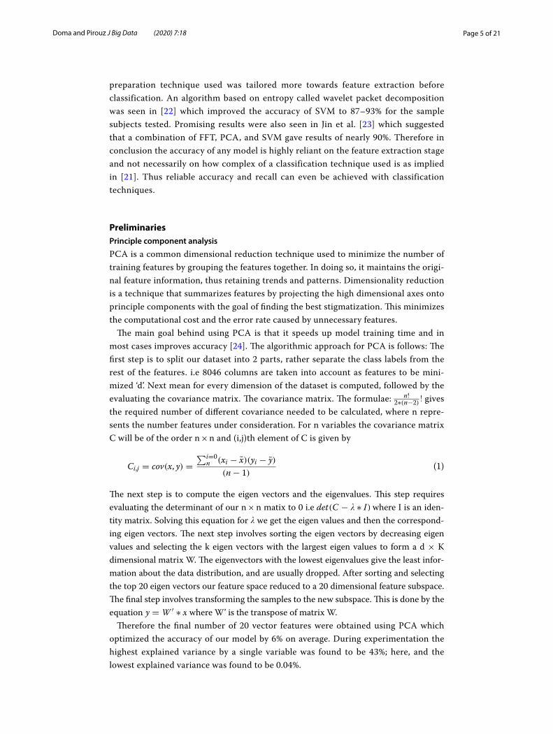
PCA is a common dimensional reduction technique used to minimize the number of training features by grouping the features together. In doing so, it maintains the origi-nal feature information, thus retaining trends and patterns. Dimensionality reduction is a technique that summarizes features by projecting the high dimensional axes onto principle components with the goal of finding the best stigmatization. This minimizes the computational cost and the error rate caused by unnecessary features.

The main goal behind using PCA is that it speeds up model training time and in most cases improves accuracy [24]. The algorithmic approach for PCA is follows: The first step is to split our dataset into 2 parts, rather separate the class labels from the rest of the features. i.e 8046 columns are taken into account as features to be mini-mized ‘d’. Next mean for every dimension of the dataset is computed, followed by the evaluating the covariance matrix. The covariance matrix. The formulae: n!

2∗(n−2) ! gives the required number of different covariance needed to be calculated, where n repre-sents the number features under consideration. For n variables the covariance matrix C will be of the order n × n and (i,j)th element of C is given by

The next step is to compute the eigen vectors and the eigenvalues. This step requires evaluating the determinant of our n × n matix to 0 i.e det(C − � ∗ I) where I is an iden-tity matrix. Solving this equation for � we get the eigen values and then the correspond-ing eigen vectors. The next step involves sorting the eigen vectors by decreasing eigen values and selecting the k eigen vectors with the largest eigen values to form a d × K dimensional matrix W. The eigenvectors with the lowest eigenvalues give the least infor-mation about the data distribution, and are usually dropped. After sorting and selecting the top 20 eigen vectors our feature space reduced to a 20 dimensional feature subspace. The final step involves transforming the samples to the new subspace. This is done by the equation y = W ′ ∗ x where W’ is the transpose of matrix W.

Therefore the final number of 20 vector features were obtained using PCA which optimized the accuracy of our model by 6% on average. During experimentation the highest explained variance by a single variable was found to be 43%; here, and the lowest explained variance was found to be 0.04%.

(1)Ci,j = cov(x, y) =

∑i=0n (xi − x)(yi − y)

(n− 1)


Naive Bayes

The Naive Bayes classifier assumes that the presence of a selected feature in class is unre-lated to the presence of the other feature belonging to other classes. Even if these options depend upon one another or upon the existence of the opposite options, all of those properties contribute to the chance [25]. Naive Bayes is particularly suitable for when the dimensionality is higher. Therefore, we are testing this classifier in the experiment. Naive Bayes model is significantly helpful for wide sets with many attributes [26]. Along with its simplicity, Naive Bayes model may surpass even extremely subtle classification techniques.

The naive Bayes equation is explained below

Naive Bayes equation can be extended to real-valued attributes, most typically by assuming a normal distribution. Different functions do not estimate the distribution of the info, but relies on the estimation of the mean and therefore the variance from the information. The Naive Bayes algorithm requires a joint probability P(A,B). This is the probability of both A and B occuring given as at the same time it must be considered that the variables are independent of each other:

Equation 2 represents the Gaussian Naive Bayes used here and the reason behind using Gaussian Naive Bayes was due to the slight Gaussian distribution of the features.

Logistic regression

It is another classification algorithm available for both multi-class and binary class clas-sification. Logistic Regression performs discrete categorization of sampled data, for a binary class (pass or fail) within a decision boundary. The analogy between the linear and logistic regression can be explained with the regression hypothesis

where 3 represents the logistic regression hypothesis and 4 is the linear regression hypotheses where theta represents the parameters. To determine the split between

(2)P(A|B) =P(B|A)P(A)

P(B)

(3)P(A|B) = P(A|B) ∗ P(B)

(4)P(xi|y) =1

√

2πσ 2y

exp

(

−(xi − µy)2

2σ 2y

)

(5)hθ (x) =1

1+ e(−θT x)

(6)hθ (x) = (−θTx)

(7)f (z) =

{

θ0 + θ1x1 + θ2x2 + θ19x19 ≤ 01, otherwise


classes, it is ideal to use all features, however with PCA we limit the features from 8064 to just 20 as seen in 5, where f(z) gives the class for the sample.

K‑nearest neighbor

When we perform classification using K-nearest neighbor (KNN), the algorithm is essentially giving a way to extract the majority vote which decides whether the observa-tion belongs to a certain K-similar instance. For this, in any dimensional space, Euclid-ean distance is used. Since KNN is a non-parametric classification algorithm, it assigns labels to previously un-sampled points, generally it has a lower efficiency as the size of the data increases [27]; thus, further promoting the need for a feature decomposition algorithm. The performance is fully-dependent on the value of k, as such the model was created to test over the values of k, which was done through iterations above k-fold cross validation from 0 to 5, where the values of k for KNN ranged from 2 to 50. This method-ology was suggested as it is not easy to select a proper value of k theoretically, unless an exhaustive search using expensive techniques is performed [25].

Support Vector Machines

Support Vector Machines (SVM) are supervised linear classification models which makes use of hyperplanes (i.e. the plane of separation between classes). To sample the data, EEG channel samples are plotted in space where the number axes determine the different features. Separate categories of data are divided through a separation which is as wide as viable. When training the model, the vector w and the bias b must be esti-mated by the solution to a quadratic equation [12]. Hence, SVM can be implemented in polynomial time, which makes it a p-complete problem.

where b represents a two-dimensional plane, the margin of separation is expressed as follows

Considering only two dimensions, the hyperplane equation will be for each vector (6). This simplifies the learning problem of the SVM by transforming it into an optimization problem where 2

‖w‖ represents the margin of separation stated by

Using these two equations, we have the following simplified equation as given below:

(8)wTxi + b ≥ 1 for xi ∈ CLASSA

(9)wTxi + b ≤ 1 for xi ∈ CLASSB

(10)yi � wTx + b �

(11)maximize

wMax(w) 2

�w�

subject to W · xi + b ≥ 1 if yi = 1

(12)maximize

wMax(w) 2

�w�

subject to W · xi + b ≤ −1 for i = 1 to N


Decision trees

A decision tree is a kind of hierarchical class selection support tool that uses a tree-like graph or model of choices and their attainable consequences [25] (i.e. bifurcation based on the decision taken at each level) together with accident outcomes, cost, and utility. A decision tree a technique which only uses the conditional management statements for class separation. A decision tree could be a flowchart-like structure where every internal node represents a “test” on an attribute (e.g. whether or not a coin flip comes up heads or tails). Every branch represents the result of the check, and every leaf node represents a category label (the decision is made once all attributes are computed). The paths from root to leaf represent classification rules. Decision Trees are primarily based learning algorithms that are among the simplest and mostly-used supervised learning strategies . Tree primarily based strategies empower prophetical models with high accuracy, stabil-ity and simple interpretation. In contrast to linear models, they map non-linear relation-ships quite well. They are adaptable at determining any reasonably downside at hand (classification or regression). Decision Tree classification algorithms are known as Clas-sification and Regression Trees (CART) [3].

Parameter tuning

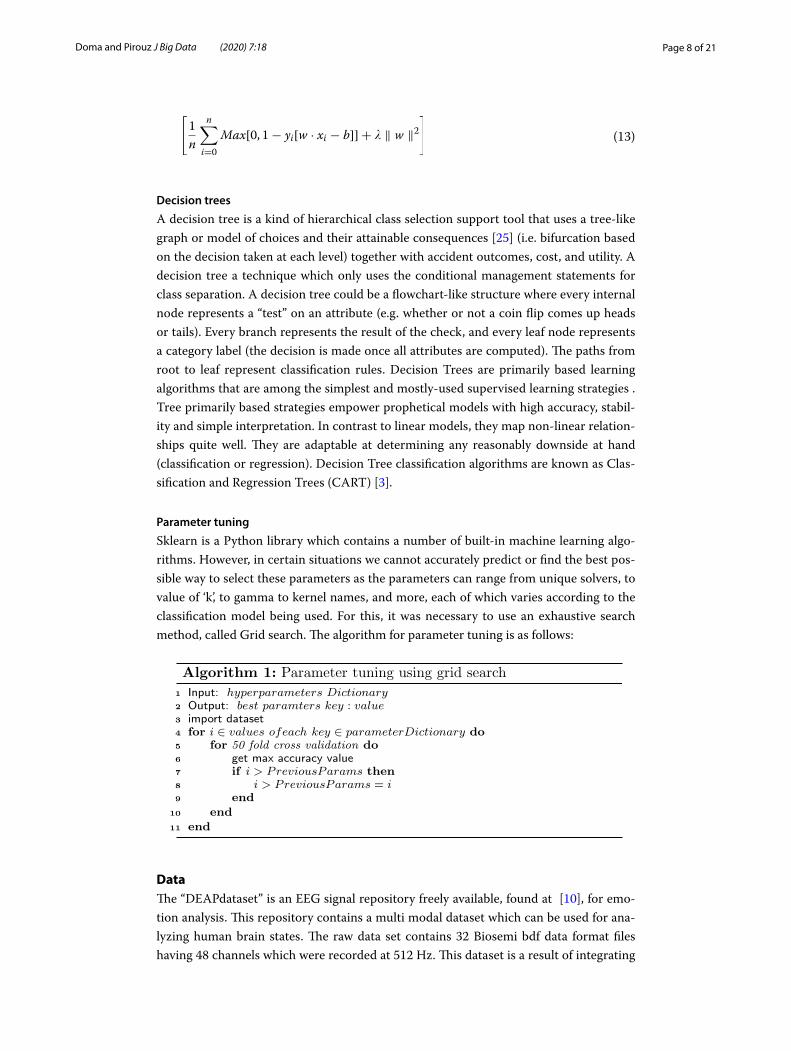
Sklearn is a Python library which contains a number of built-in machine learning algo-rithms. However, in certain situations we cannot accurately predict or find the best pos-sible way to select these parameters as the parameters can range from unique solvers, to value of ‘k’, to gamma to kernel names, and more, each of which varies according to the classification model being used. For this, it was necessary to use an exhaustive search method, called Grid search. The algorithm for parameter tuning is as follows:

Algorithm 1: Parameter tuning using grid search1 Input: hyperparameters Dictionary2 Output: best paramters key : value3 import dataset4 for i ∈ values ofeach key ∈ parameterDictionary do5 for 50 fold cross validation do6 get max accuracy value7 if i > PreviousParams then8 i > PreviousParams = i9 end

10 end11 end

DataThe “DEAPdataset” is an EEG signal repository freely available, found at [10], for emo-tion analysis. This repository contains a multi modal dataset which can be used for ana-lyzing human brain states. The raw data set contains 32 Biosemi bdf data format files having 48 channels which were recorded at 512 Hz. This dataset is a result of integrating

(13)

[

1

n

n∑

i=0

Max[0, 1− yi[w · xi − b]] + � � w �2

]


3 database recordings at distinct locations namely, Geneva Switzerland, Twente Nether-lands, London United Kingdom. This shows the variety of the data as different sampling rates were used and different types of tests were conducted. Aggregating this data into 1 comprehensive dataset shows the large volume of the data, especially when the face recordings are used for predictive purposes. It is ensured that this raw data cannot be tampered with as files are made to be read only, furthermore the collection of data was done 5 times for each test to ensure trustworthy data. Each of the two zip folders contain 32 participants each with the data stored in a 3D matrix representation (40 × 40 × 8064) representing video/trial × channel × data, with the numeric class value labels saved on the same file as a 2D matrix. After reformatting the data during data preparation the updated dataset contained 204,800 × 8065. A total of 11.2 GB worth of sampled EEG data with an additional 15 GB raw face recording data is available for reference.

The metadata folder contains 4 important metadata files describing the way the data was collected and the ratings they gave during the experiment after each of the 32 par-ticipants had 40 min-long sessions. “Wheel slice” was an important column which tells us exactly what the subject is feeling at that particular instant. The integer values for this range from 1 to 16. Similarly, the 32 participants were prompted to rate their feelings based on the honor system in terms of 1–9, representing their degree of arousal, valence, familiarity, and dominance.

Along with the raw data, the dataset includes a preprocessing script, which is available in either Matlab and pickled Python formats. This script contains the subject data in two arrays, one for data and the other for labels (arousal, liking, dominance). This data ena-bles applying classification algorithms without worrying about the preprocessing phase. This research uses the pre-processed version to compare the initial accuracy of classic classification algorithms. EEG data collected from 32 patients can be read by using the pickle library in Python.

MethodsExploratory Data Analysis (EDA) is the first step in understanding the type of data that is processed along with how the data can be used for developing a solid foundation on which we can build prediction models. Here, one creates a sense of the information that can be used to fire queries one wishes to raise to border their understanding. Similarly, one can control the knowledge sources to urge the answers they seek. The basic idea is to perform an analysis that can help in deciding what techniques are to be used to process, manipulate, normalize and extract information from the data that can help in finding better approaches while implementing predictive models.

Since the “DEAP dataset” contains the four distinct ratings for each of the 40 videos, it is possible to visualize how exactly the distribution of the ratings are, this also facili-tated the detection of any biases towards any particular rating. In this case, a smaller bias would help achieve better accuracy classification, as larger bias makes machine learning models sway to predict the biased class.

After reading the pickled data into different files containing the encoded data from the numpy arrays using one hot encoding representing the different class values, it is possible to perform different binary class classifications for each of the four distinct categories of valence, arousal, dominance and liking. The subjects rated each of the


60 s video based on these criteria on a scale of 1 to 9. Therefore, one hot encoding was used to round all values below 5 to 0 and those above the threshold of 5 to 1, thus allowing a binary classifier. The classes were labeled as ‘unhappy’, ‘happy/joyful’, ‘calm/board’, ‘stimulated/excited’, ‘submissive’, ‘empowered’, ‘thumbs up’, ‘thumbs down’ representing both the positive and negative emotion of that criteria. The fol-lowing are the different machine learning techniques used, once the one hot encoding was complete

The DEAP dataset [7] gives the preprocessed data in the form of a saved pickle file. Loading the file gives two different arrays named labels and data. The labels were auto encoded into four different files, each representing an emotion. The data was extracted separately for each subject and stored the EEG epoch channel data in from each subject into a single file called “collected_features.dat”. The labels for the classes and the actual data were separated from each other in different files. This separation was performed before cross validation and limited the number of features to 20 when selecting each of the classification models. Grid search then gave a detailed report of the classification accuracy, f-score, precision, and recall. This approach yielded results within the range of 50 to 65%.

This approach was done on a preliminary basis in order to get baseline results for the modification and optimization phase further ahead. According to the DEAP dataset, the epoch data was segmented into 60 s trials, thus it is not very clear where the correct emotion may arise within this 60 s of data. One hypothesis is that within the first few seconds, the subject experienced feelings prior to watching the music, i.e continuing the same state of emotion before the trial. Similarly, the last few seconds could provide much better features as the subject can now anticipate the events in the video. Thus, leading to the question of segmenting the data into 15sec ∗ 4partitions corresponding to 1 subject trial. These segments were uploaded to the google cloud clustered architecture. With the help of joblib a Apache spark backend library, a distributed GridSearch was done over the spark cluster. The number of jobs created for each machine learning algorithm was 3. This boosted the execution time. Each segment was tested separately to check for accuracy, f-score, precision and recall for each of the 4 classes. Assuming that if, any one segment shows better results than the others then our hypothesis is that the segment of epoch data giving these results is related to an important part of the trial video which best brings out the corresponding emotional state.

Apart from this, the objective of PCA was to minimize the features. This is due to the fact that even though all the channel data from each of the 40 channels were used, PCA did not seem to be very effective because of the fluctuation in the epoch signals. Therefore, a techniques adapted from [28, 29] was performed to calculate the features rather than the raw signal epoch data. These features include mean, mode, median as F1, F2 and F3 respectively; as well as the range, largest-smallest element within the segmented range as F4, F5, F6 variance respectively. PCA then selected the features that were taken from the result of the co-variance matrix, i.e the higher weighted ele-ments. This approach achieved better results, as expected and tested by the literature. It is important to note that such modification is done before using any classification techniques. Grid search and k-fold cross-validation helped in fine tuning the param-eters to get the best possible results. At this stage, five different classifiers were tested.


SetupThe experimentation done with the data sets mentioned in “Methods” section only, thus additional external hardware setup was not required although a spark cluster on google cloud was utilised to distribute the workload. This was done using parallel_back-end function on the Joblib Apache Spark Backend. Setup seen in [30], since streaming raw epoch data from patients is not within the scope of this research. software packages including Anaconda 2019.03 Release for python 3.6, pyspark version 2.4.4 and EEGlab toolbox for Matlab rev. 9.0.7.6. The python libraries used were matplotlib, numpy, pan-das, pytorch, sklearn v 0.21, to name a few. These libraries were installed on the conda environment using “conda install” and “pip install”. the “.mat” files from “DEAP” were read and exported as csv files through EEGlab The following results obtained in “Setup” section, were produced on Ubuntu 18.01 using 7th Generation intel@ Core i7 processor with 8GB RAM.

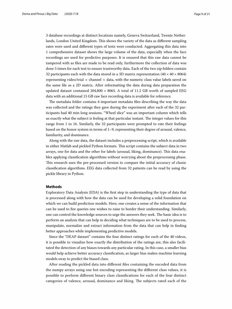
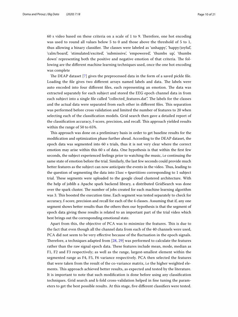
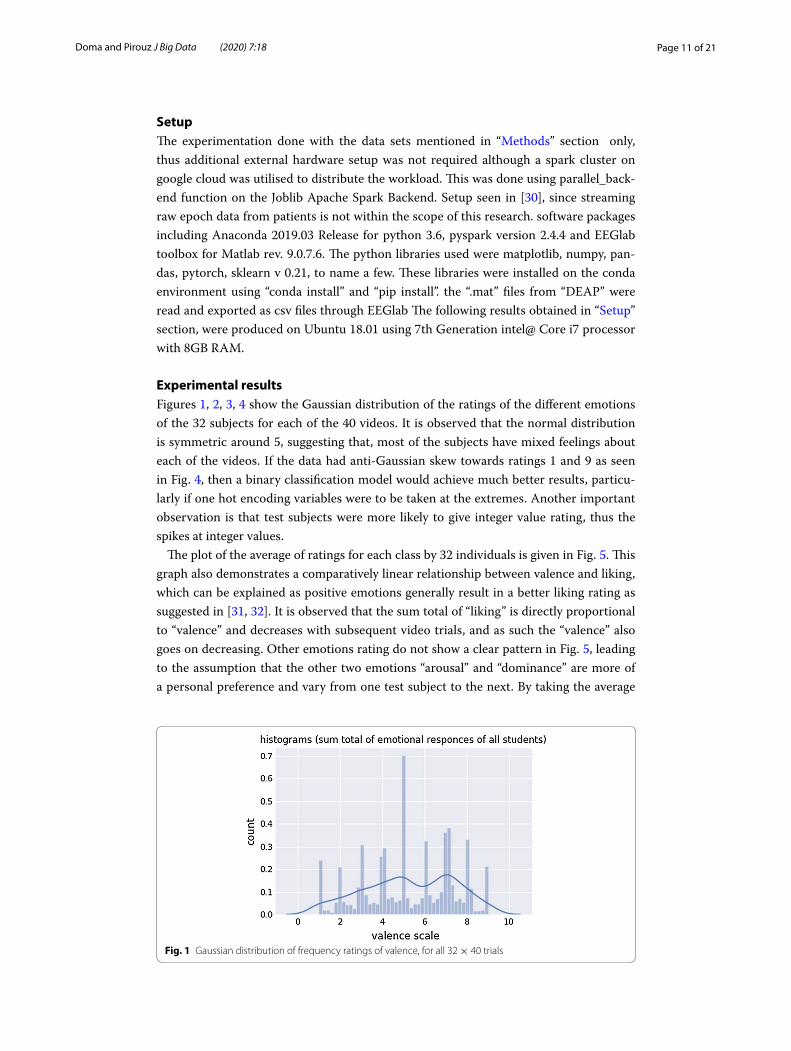
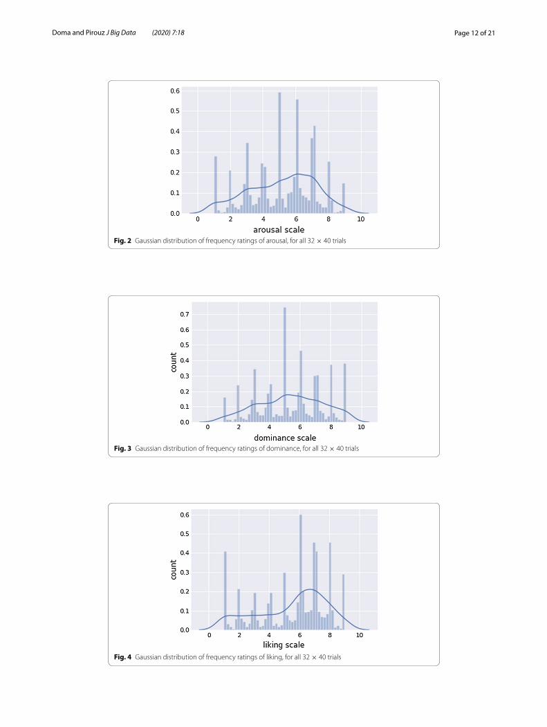
Experimental resultsFigures 1, 2, 3, 4 show the Gaussian distribution of the ratings of the different emotions of the 32 subjects for each of the 40 videos. It is observed that the normal distribution is symmetric around 5, suggesting that, most of the subjects have mixed feelings about each of the videos. If the data had anti-Gaussian skew towards ratings 1 and 9 as seen in Fig. 4, then a binary classification model would achieve much better results, particu-larly if one hot encoding variables were to be taken at the extremes. Another important observation is that test subjects were more likely to give integer value rating, thus the spikes at integer values.

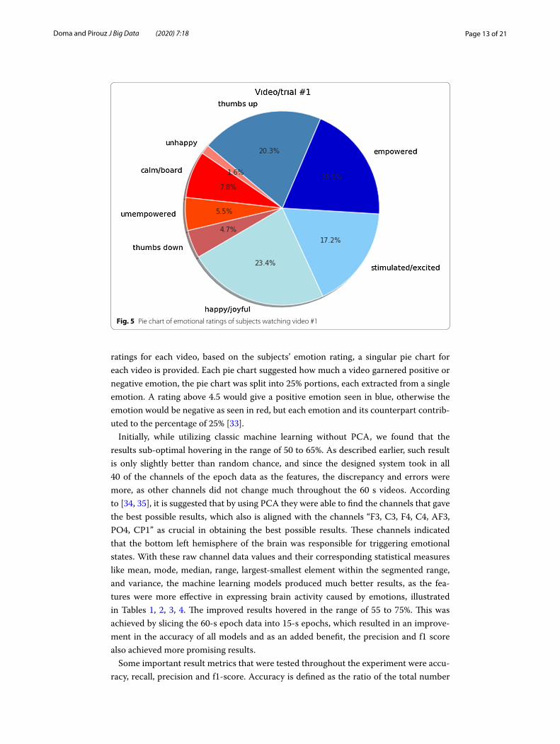
The plot of the average of ratings for each class by 32 individuals is given in Fig. 5. This graph also demonstrates a comparatively linear relationship between valence and liking, which can be explained as positive emotions generally result in a better liking rating as suggested in [31, 32]. It is observed that the sum total of “liking” is directly proportional to “valence” and decreases with subsequent video trials, and as such the “valence” also goes on decreasing. Other emotions rating do not show a clear pattern in Fig. 5, leading to the assumption that the other two emotions “arousal” and “dominance” are more of a personal preference and vary from one test subject to the next. By taking the average

Fig. 1 Gaussian distribution of frequency ratings of valence, for all 32 × 40 trials


Fig. 2 Gaussian distribution of frequency ratings of arousal, for all 32 × 40 trials

Fig. 3 Gaussian distribution of frequency ratings of dominance, for all 32 × 40 trials

Fig. 4 Gaussian distribution of frequency ratings of liking, for all 32 × 40 trials


ratings for each video, based on the subjects’ emotion rating, a singular pie chart for each video is provided. Each pie chart suggested how much a video garnered positive or negative emotion, the pie chart was split into 25% portions, each extracted from a single emotion. A rating above 4.5 would give a positive emotion seen in blue, otherwise the emotion would be negative as seen in red, but each emotion and its counterpart contrib-uted to the percentage of 25% [33].

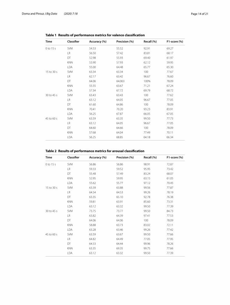
Initially, while utilizing classic machine learning without PCA, we found that the results sub-optimal hovering in the range of 50 to 65%. As described earlier, such result is only slightly better than random chance, and since the designed system took in all 40 of the channels of the epoch data as the features, the discrepancy and errors were more, as other channels did not change much throughout the 60 s videos. According to [34, 35], it is suggested that by using PCA they were able to find the channels that gave the best possible results, which also is aligned with the channels “F3, C3, F4, C4, AF3, PO4, CP1” as crucial in obtaining the best possible results. These channels indicated that the bottom left hemisphere of the brain was responsible for triggering emotional states. With these raw channel data values and their corresponding statistical measures like mean, mode, median, range, largest-smallest element within the segmented range, and variance, the machine learning models produced much better results, as the fea-tures were more effective in expressing brain activity caused by emotions, illustrated in Tables 1, 2, 3, 4. The improved results hovered in the range of 55 to 75%. This was achieved by slicing the 60-s epoch data into 15-s epochs, which resulted in an improve-ment in the accuracy of all models and as an added benefit, the precision and f1 score also achieved more promising results.

Some important result metrics that were tested throughout the experiment were accu-racy, recall, precision and f1-score. Accuracy is defined as the ratio of the total number

Fig. 5 Pie chart of emotional ratings of subjects watching video #1


Table 1 Results of performance metrics for valence classification

Time Classifier Accuracy (%) Precision (%) Recall (%) F1‑score (%)

0 to 15 s SVM 54.53 55.52 92.91 69.27

LR 56.50 57.42 83.81 68.17

DT 52.98 55.93 69.40 61.97

KNN 53.90 57.93 62.12 59.95

LDA 55.00 64.48 65.77 65.30

15 to 30 s SVM 63.34 63.34 100 77.67

LR 62.17 63.42 96.67 76.60

DT 64.06 64.063 100% 78.09

KNN 55.55 63.67 71.21 67.24

LDA 57.34 67.72 69.79 68.72

30 to 45 s SVM 63.43 63.43 100 77.62

LR 63.12 64.05 96.67 77.05

DT 61.60 64.86 100 78.09

KNN 70.41 70.20 93.23 83.91

LDA 56.25 67.87 66.05 67.05

45 to 60 s SVM 63.59 63.35 99.50 77.73

LR 63.12 64.05 96.67 77.05

DT 64.60 64.66 100 78.09

KNN 57.68 64.04 77.49 70.11

LDA 56.25 68.85 64.18 66.34

Table 2 Results of performance metrics for arousal classification


0 to 15 s SVM 56.86 56.86 98.91 72.87

LR 59.33 59.52 95.95 73.42

DT 55.48 57.49 83.24 68.07

KNN 52.95 59.95 63.15 61.05

LDA 55.62 55.77 97.12 70.45

15 to 30 s SVM 63.39 63.88 99.56 77.87

LR 64.54 64.53 99.26 78.19

DT 63.35 65.10 92.78 76.38

KNN 59.81 63.91 85.60 73.31

LDA 63.12 63.32 99.50 77.39

30 to 45 s SVM 73.75 73.77 99.50 84.73

LR 63.82 64.39 97.41 77.53

DT 64.06 64.06 100 78.09

KNN 58.88 63.73 83.02 72.11

LDA 63.28 63.46 99.26 77.42

45 to 60 s SVM 63.59 63.67 99.50 77.66

LR 64.82 64.49 77.05 77.95

DT 64.53 64.44 99.96 78.26

KNN 63.35 69.35 99.75 77.66

LDA 63.12 63.32 99.50 77.39


Table 3 Results of performance metrics for dominance classification


0 to 15 s SVM 64.53 64.52 100 78.09

LR 64.30 64.42 97.00 77.42

DT 50.62 68.73 37.50 47.87

KNN 59.33 67.93 70.02 69.47

LDA 57.81 57.48 99.09 72.78

15 to 30 s SVM 67.65 67.65 100 80.07

LR 68.36 69.56 96.95 81.01

DT 65.01 70.58 85.54 77.30

KNN 63.59 70.20 83.05 76.86

LDA 67.5 67.77 99.06 80.05

30 to 45 s SVM 67.18 67.72 99.55 77.66

LR 68.08 69.66 96.85 80.85

DT 67.84 71.20 97.50 79.99

KNN 62.64 69.85 81.69 75.31

LDA 66.56 67.35 98.96 79.88

45 to 60 s SVM 66.25 67.30 100 79.62

LR 67.73 69.47 94.94 80.22

DT 71.73 69.73 98.40 82.17

KNN 63.12 68.03 86.45 76.14

LDA 66.67 67.40 98.34 79.99

Table 4 Results of performance metrics for liking classification


0 to 15 s SVM 64.37 64.37 96.96 78.27

LR 66.43 66.56 98.56 80.42

DT 61.12 66.40 85.00 72.80

KNN 62.24 67.96 81.36 74.06

LDA 64.45 64..56 99.51 78.95

15 to 30 s SVM 67.76 67.76 100 80.44

LR 68.32 69.33 96.77 81.71

DT 68.05 68.07 100 81.01

KNN 65.48 69.25 88.54 77.76

LDA 67.03 67.29 99.06 80.15

30 to 45 s SVM 71.51 70.45 99.76 83.48

LR 69.54 69.08 99.30 81.48

DT 68.08 68.08 100 81.01

KNN 74.28 77.49 98.05 86.57

LDA 67.50 67.50 99.53 80.45

45 to 60 s SVM 67.18 68.18 100 80.07

LR 68.08 68.05 98.95 80.85

DT 67.78 68.09 99.30 80.79

KNN 63.12 68.03 86.45 76.16

LDA 67.34 67.34 99.76 80.40


of correct predictions achieved by a model to the measure of total predictions done, regardless of correct or incorrect predictions. Precision is given as

where TP stands for true positives, i.e. how many true correct predictions were actually done and FP stands for false positives, i.e. how many predictions were incorrectly classi-fied as belonging to that class, which could also be explained as the incorrectly predicted positives measure. The recall score is given as follows

Also called as sensitivity, or the true positive rate ratio of correct predictions to the total number of positives examples. The last measure is F1 score which combines precision and recall, a good F1 score suggests a low false positives and low false negatives. A per-fect F1 score will be 1 while the model is a total failure at 0. The formulae for F1 score is given as follows

Thus higher the percent values for the performance metrics indicates a better model. The performance measures increase as long as the number of the samples that are cho-sen are correctly classified rise as well. Here in this research we are looking for a high accuracy and F1 score, which can help others know which algorithms would be the best for experimenting on human subjects. Tables 1, 2, 3, 4 present the performance meas-ures obtained after running each binary classifier through four segments of the 60 s of the music video. Through general observation, the initial time from 0 to 15 s for all binary classification models experienced a lower accuracy range of 50 to 66% followed by 15 to 30 s then by 45 to 60 s, and finally 30 to 45 s. An in-depth analysis of Table 1, 2, 3, 4 demonstrates that segmenting the data is useful in obtaining better results as well as in finding out which sections of the recorded data have the most brain activity cor-responding to the emotions. Of all the results, Table 4 represents better results. KNN resulted in an accuracy of 74.25% as the best possible result obtained among all model and their parameters. Grid search was able to converge with the best parameters being leaf size: 1, n nearest neighbor: 10, weights: distance. The recall, precision, and F1 score for theses parameters were much larger with the recall score being 86.57%. Similarly for SVM, which achieved an accuracy of 71.51% and the F1 score of 83.48% in the same split of epoch data, the best possible parameters were found to be a polynomial kernel with degree at 3 and gamma at 0.16. In all Tables 1, 2, 3, 4, the best parameters were achieved by grid search. Logistic Regression converged with penalty being l1 and the inverse regularization strength was found to be 1. Decision trees also performed well, with a maximum accuracy reaching 68% and an F1 score being 77%. For decision trees the best accuracy and recall was max depth being 3 and the minimum split samples were 10. An important point to be noted is that the recall scores are high ranging from 85 to 100% due to correctly predicted emotion among the positive and negative emotional states,

(14)Precision =TP

TP + FP

(15)Recall =TP

TP + FN

(16)F1 = 2 ∗precision ∗ recall

precision+ recall


however all F1 scores suffered a low precision suggesting that among all the subjects who had a positive emotion, the number of subjects that were correctly labeled with a positive emotion was less ranging from the low 60 s to the low 70 s.

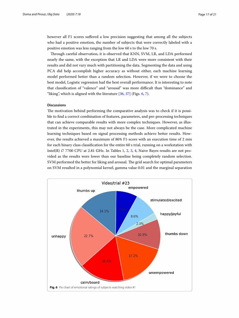
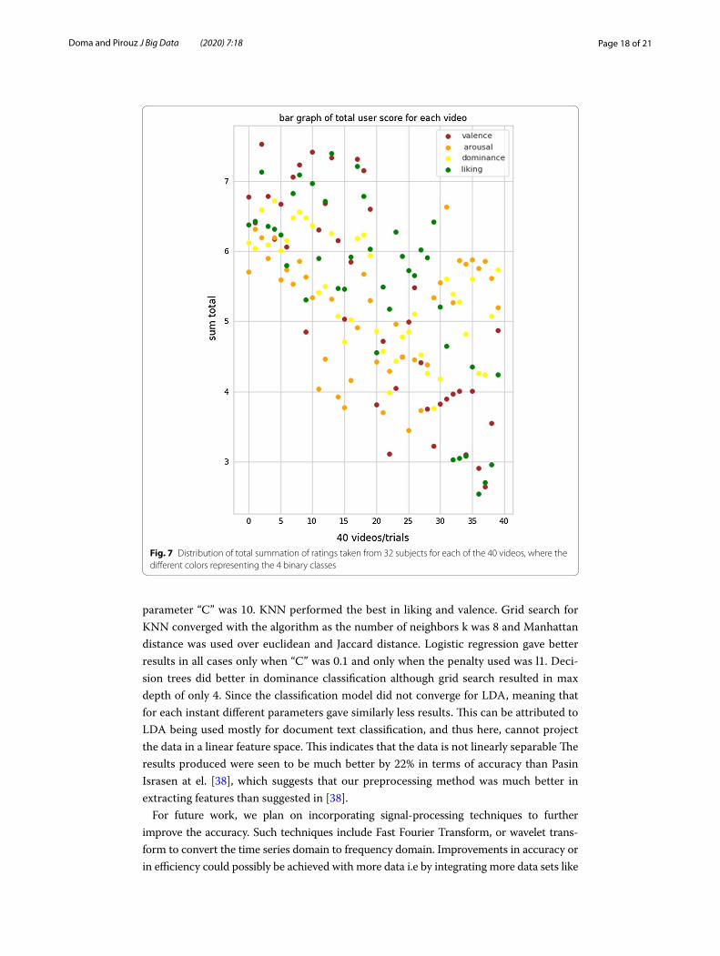
Through careful observation, it is observed that KNN, SVM, LR, and LDA performed nearly the same, with the exception that LR and LDA were more consistent with their results and did not vary much with partitioning the data. Segmenting the data and using PCA did help accomplish higher accuracy as without either, each machine learning model performed better than a random selection. However, if we were to choose the best model, Logistic regression had the best overall performance. It is interesting to note that classification of “valence” and “arousal” was more difficult than “dominance” and “liking”, which is aligned with the literature [36, 37] (Figs. 6, 7).

Discussions

The motivation behind performing the comparative analysis was to check if it is possi-ble to find a correct combination of features, parameters, and pre-processing techniques that can achieve comparable results with more complex techniques. However, as illus-trated in the experiments, this may not always be the case. More complicated machine learning techniques based on signal processing methods achieve better results. How-ever, the results achieved a maximum of 86% F1-score with an execution time of 2 min for each binary class classification for the entire 60 s trial, running on a workstation with Intel(R) i7 7700 CPU at 2.81 GHz. In Tables 1, 2, 3, 4, Naive Bayes results are not pro-vided as the results were lower than our baseline being completely random selection. SVM performed the better for liking and arousal. The grid search for optimal parameters on SVM resulted in a polynomial kernel, gamma value 0.01 and the marginal separation

Fig. 6 Pie chart of emotional ratings of subjects watching video #1


parameter “C” was 10. KNN performed the best in liking and valence. Grid search for KNN converged with the algorithm as the number of neighbors k was 8 and Manhattan distance was used over euclidean and Jaccard distance. Logistic regression gave better results in all cases only when “C” was 0.1 and only when the penalty used was l1. Deci-sion trees did better in dominance classification although grid search resulted in max depth of only 4. Since the classification model did not converge for LDA, meaning that for each instant different parameters gave similarly less results. This can be attributed to LDA being used mostly for document text classification, and thus here, cannot project the data in a linear feature space. This indicates that the data is not linearly separable The results produced were seen to be much better by 22% in terms of accuracy than Pasin Israsen at el. [38], which suggests that our preprocessing method was much better in extracting features than suggested in [38].

For future work, we plan on incorporating signal-processing techniques to further improve the accuracy. Such techniques include Fast Fourier Transform, or wavelet trans-form to convert the time series domain to frequency domain. Improvements in accuracy or in efficiency could possibly be achieved with more data i.e by integrating more data sets like

Fig. 7 Distribution of total summation of ratings taken from 32 subjects for each of the 40 videos, where the different colors representing the 4 binary classes


SEED in combination with DEAP [39]. Introduction of complex Deep or Convolutional Neural Networks may provide an added boost to accuracy as manual selection of features is time-consuming and may not necessarily be the best approach. As neural networks auto tune the features to provide the best results, the performance measures are expected to be significantly more.

ConclusionThe main goal was to discover how neurophysiological mechanisms are able to drive an individuals to experience emotion, and figure out which portions of the brain carry data related to different emotions. This was achieved by performing classic machine leaning techniques of SVM, Naive Bayes, Decision Trees, Logistic regression, KNN and LDA, each of which achieved an accuracy of between 55 and 75% and an F1 score ranging from 70 to 86%. The classification techniques did not significantly outperform one another; how-ever, the best result was achieved during KNN classification for “Liking”. in terms of highest accuracy achieved the order of classification algorithms in descending order is: KNN, SVM, Decision trees, Logistic Regression, and LDA. The statistical features of the channels and raw channel data corresponding to the back left hemisphere of the brain was seen to have more activity and thus, dimensional reduction was done alongside partitioning the epoch channel data of 60 s into four 15-s chunks to get the best possible selection features, achiev-ing an improved accuracy. Furthermore PySpark proved useful for distributing the work-load of hyper parameter tuning. The experiments could further be scaled to account for more emotions or for a combination of emotions without compromising F1 and accuracy.

The experimentation suggests that classic machine learning algorithms achieve reason-able results and identify information regarding important epoch channels that are responsi-ble for emotional states.

AbbreviationsEEG: Electroencephalogram; BCI: Brain computer interfaces; SVM: Support Vector Machines; KNN: K-nearest neighbor; EN: Elastic net regression; CCEMRC: Critical care EEG monitoring research consortium; cEEG: Continuous EEGs; SLIM: Sparse linear integer model; LDA: Linear discriminant analysis; CART : Classification and regression trees; EDA: Exploratory data analysis.

AcknowledgementsNot applicable.

Authors’ contributionsVD performed the primary literature review, ran the experiments, and drafted the manuscript. MP worked closely with VD on the research and experiment design and result analysis as well as finalizing the manuscript. Both authors read and approved the final manuscript.

FundingThis research has been partially funded by the College of Science and Mathematics, and a Grant from Amazon Web Services.

Availability of data and materialsThe dataset used in this study is available through [10].

Competing interestsThe authors declare that they have no competing interests.

Received: 9 September 2019 Accepted: 17 February 2020


References 1. Daros A, Zakzanis K, Ruocco A. Facial emotion recognition in borderline personality disorder. Psychol Med.

2013;43:1953–63. 2. Schaaff K, Schultz T. Towards emotion recognition from electroencephalographic signals. In: 2009 3rd international

conference on affective computing and intelligent interaction and workshops. New York: IEEE; 2009. p. 1–6. 3. Bertsimas D, Dunn J, Paschalidis A. Regression and classification using optimal decision trees. In: 2017 IEEE MIT

undergraduate research technology conference (URTC). 2017. p. 1–4. 4. Jiahui Pan, Yuanqing Li, Jun Wang. An EEG-based brain–computer interface for emotion recognition. In: 2016 inter-

national joint conference on neural networks (IJCNN). 2016. p. 2063–67. 5. Pantic M, Rothkrantz LJ. Automatic analysis of facial expressions: the state of the art. IEEE Trans Pattern Anal Mach

Intell. 2000;22:1424–45. 6. Osisanwo F, et al. Supervised machine learning algorithms: classification and comparison. Int J Comput Trends

Technol. 2017;48:128–38. 7. Kalhori SRN, Zeng X-J. Evaluation and comparison of different machine learning methods to predict outcome of

tuberculosis treatment course. J Intell Learn Syst Appl. 2013;5:184. 8. Vanitha V, Krishnan P. Real time stress detection system based on EEG signals. 2016. 9. Liao C-Y, Chen R-C, Tai S-K. Emotion stress detection using eeg signal and deep learning technologies. In: 2018 IEEE

international conference on applied system invention (ICASI). New York: IEEE; 2018. p. 90–3. 10. Koelstra S, et al. Deap: a database for emotion analysis; using physiological signals. IEEE Trans Affect Comput.

2011;3:18–31. 11. Jia W et al. Electroencephalography (eeg)-based instinctive brain-control of a quadruped locomotion robot. In: 2012

annual international conference of the IEEE engineering in medicine and biology society. New York: IEEE; 2012. p. 1777–81.

12. Fakhruzzaman MN, Riksakomara E, Suryotrisongko H. Eeg wave identification in human brain with emotiv epoc for motor imagery. Procedia Comput Sci. 2015;72:269–76.

13. Shariat S, Pavlovic V, Papathomas T, Braun A, Sinha P. Sparse dictionary methods for EEG signal classification in face perception. In: 2010 IEEE international workshop on machine learning for signal processing. New York: IEEE; 2010. p. 331–6.

14. Tabar YR, Halici U. A novel deep learning approach for classification of EEG motor imagery signals. J Neural Eng. 2016;14:016003.

15. Chambon S, Thorey V, Arnal PJ, Mignot E, Gramfort A. A deep learning architecture to detect events in EEG signals during sleep. In: 2018 IEEE 28th international workshop on machine learning for signal processing (MLSP). New York: IEEE; 2018. p. 1–6.

16. Bashivan P, Rish I, Yeasin M, Codella N. Learning representations from EEG with deep recurrent-convolutional neural networks. arXiv preprint arXiv :1511.06448 . 2015.

17. Thomas J, et al. EEG classification via convolutional neural network-based interictal epileptiform event detection. In: 2018 40th annual international conference of the IEEE engineering in medicine and biology society (EMBC). New York: IEEE; 2018. p. 3148–51.

18. Pion-Tonachini L, Kreutz-Delgado K, Makeig S. Iclabel: an automated electroencephalographic independent compo-nent classifier, dataset, and website. NeuroImage. 2019;198:181–97.

19. Struck AF, et al. Comparison of machine learning models for seizure prediction in hospitalized patients. Ann Clin Transl Neurol. 2019;67:1239–47.

20. Belakhdar I, Kaaniche W, Djmel R, Ouni B. A comparison between ANN and SVM classifier for drowsiness detection based on single EEG channel. 2016. p. 443–6.

21. Li S, Feng H. EEG signal classification method based on feature priority analysis and CNN. 2019. p. 403–6. 22. Zhiwei L, Minfen S. Classification of mental task EEG signals using wavelet packet entropy and SVM. 2007. p. 906–9. 23. Jin J, Wang X, Wang B. Classification of direction perception EEG based on PCA-SVM, vol. 2. 2007. p. 116–20. 24. Song F, Guo Z, Mei D. Feature selection using principal component analysis. In: 2010 international conference on

system science, engineering design and manufacturing informatization, vol. 1. 2010. p. 27–30. 25. Pedregosa F, et al. Scikit-learn: machine learning in python. J Mach Learn Res. 2011;12:2825–30. 26. Rajaguru H, Prabhakar SK. Non linear ica and logistic regression for classification of epilepsy from eeg signals. In:

2017 international conference of electronics, communication and aerospace technology (ICECA), vol. 1. 2017. p. 577–80.

27. Bablani A, Edla DR, Dodia S. Classification of EEG data using k-nearest neighbor approach for concealed information test. Procedia Comput Sci. 2018;143:242–9.

28. Tripathi S, Acharya S, Sharma RD, Mittal S, Bhattacharya S. Using deep and convolutional neural networks for accu-rate emotion classification on deap dataset. In: Twenty-ninth IAAI conference. 2017.

29. Placidi G, Di Giamberardino P, Petracca A, Spezialetti M, Iacoviello D. Classification of emotional signals from the deap dataset. In: International congress on neurotechnology, electronics and informatics, vol. 2. SCITEPRESS; 2016. p. 15–21.

30. WeichenXu123 & mengxr. Spark-Sklearn repo. 2018. https ://githu b.com/datab ricks /spark -sklea rn. 31. Oishi S, Kurtz JL. The positive psychology of positive emotions: an avuncular view. Designing positive psychology:

taking stock and moving forward. 2011. p. 101–14. 32. Kort B, Reilly R, Picard RW. An affective model of interplay between emotions and learning: reengineering educa-

tional pedagogy-building a learning companion. In: Proceedings IEEE international conference on advanced learn-ing technologies. New York: IEEE; 2001. p. 43–6.

33. Liu W, Zheng W-L, Lu B-L. Emotion recognition using multimodal deep learning. In: International conference on neural information processing. Berlin: Springer; 2016. p. 521–9.

34. Dabas H, Sethi C, Dua C, Dalawat M, Sethia D. Emotion classification using EEG signals. In: Proceedings of the 2018 2nd international conference on computer science and artificial intelligence. ACM; 2018. p. 380–4.

http://arxiv.org/abs/1511.06448

https://github.com/databricks/spark-sklearn


35. Song T, Zheng W, Song P, Cui Z. EEG emotion recognition using dynamical graph convolutional neural networks. IEEE Trans Affect Comput. 2018.

36. MacIntyre PD, Vincze L. Positive and negative emotions underlie motivation for l2 learning. Stud Second Lang Learn Teach. 2017;7.

37. Shivhare SN, Khethawat S. Emotion detection from text. 2012. arXiv preprint arXiv :1205.4944. 38. Suwicha Jirayucharoensak SP-N, Israsena P. EEG-based emotion recognition using deep learning network with

principal component based covariate shift adaptation. Sci World J. 2014. Article ID 627892. 39. Zheng W-L, Zhu J-Y, Lu B-L. Identifying stable patterns over time for emotion recognition from EEG. IEEE Trans Affect

Comput. 2017.

Publisher’s NoteSpringer Nature remains neutral with regard to jurisdictional claims in published maps and institutional affiliations.

http://arxiv.org/abs/1205.4944

a comparative analysis of machine learning methods for

Documents