a companion to fourier series - دانشگاه...

1

A Companion to Fourier Series

by

Gol Mohammad Nafisi

[email protected]

Spring 2017

2

“You can't suddenly know something just by assembling a committee of words! That's it! I'll assemble your committee.”

- Professor Farnsworth

A Note to my Fellow Travelers

The aim of these notes is to (hopefully) prepare you guys for doing essential calculations you might

encounter in any areas of physics (and everyday life!) regarding the vast realm of Fourier analysis.

To do so, we are going to review the basic tools and do as many as exercises we could, since one

does not simply learn mathematics just by watching others doing it, except by doing it oneself. I will

solve a couple of exercises in each part myself to show you how things can be done, and then I will

leave some for you to solve (a brain food for you).

! You Have to Hand in the Exercises which I Marked by ☠ Sign , highlighted in red, on the Due Date.

I used Mr. Arfken’s Mathematical Methods for Physicists [7th edition], and I included the complete

problems of the book on Fourier series, attached to this note for those of you who might not have

them. I am positive that If you cooperate, as Sidney Coleman said once, “Not only God knows, I know,

and by the end of the semester, you will know”. Last but not least, if you have any questions, feel

free to email me, I’ll be glad to be of any help.

Let’s begin, shall we?

3

Prelude

The history of Fourier analysis began by the works of some great Mathematicians like d’ Alembert,

Gauss and Lagrange. It was Joseph Fourier though, who made a breakthrough in the development

of studying the heat equation, whose bold insight was that we can model all functions by

trigonometric series, which then became known as the Fourier series. The core idea is that all

functions (signals) can be expanded as the superposition of basic (Sine and Cosine) waves with

definite frequencies. We have two types of Fourier expansions: Fourier series, and Fourier

transform.

In Fourier series, we deal with periodic functions which can be written as a discrete sum of

trigonometric (or exponential) functions with definite frequencies. On the other hand, in Fourier

transform, the arbitrary function need not to be periodic and it can be written as a continuous

integral of trigonometric (or exponential) functions with a continuum of possible frequencies.

Preliminaries

Consider a function 𝒇 : domain → codomain , for which ∃ 𝑻 > 0 , such that:

1. ∀𝑥 ∈ 𝑑𝑜𝑚𝑎𝑖𝑛 ⟹ 𝑥 ± 𝑇 ∈ 𝑑𝑜𝑚𝑎𝑖𝑛 ,

2. ∀𝑥 ∈ 𝑑𝑜𝑚𝑎𝑖𝑛 ⟹ 𝑓(𝑥 ± 𝑇) = 𝑓(𝑥) .

Then f is periodic and T is its (fundamental) period. For example, the fundamental period of the

functions, 𝑠𝑖𝑛𝑛(𝑎𝑥) , 𝑐𝑜𝑠𝑛(𝑎𝑥) is 𝑇 =𝜋

|𝑎| if n is even, and 𝑇 =

2𝜋

|𝑎| if n is odd.

The function 𝒇 is odd if 𝑓(−𝑥) = −𝑓(𝑥), and it is even if 𝑓(−𝑥) = 𝑓(𝑥). Also 𝑓 can be neither, e.g.

𝑓(𝑥) = 𝐿𝑛(𝑥) .

For functions that are not intrinsically periodic, we can define a period and a period interval. For

example, one can define a period 2𝜋 for 𝑓(𝑥) = 𝑥 , where 𝑥 ∈ [−𝜋, 𝜋] .

4

Fourier trigonometric series

Consider a function 𝑓(𝑥) with the period of 𝑇 = 2𝐿 (e.g. 𝑥 ∈ [−𝐿 , 𝐿] or 𝑥 ∈ [0 , 2𝐿]). Then the

Fourier theorem states that we can write 𝑓 as:

𝑓(𝑥) = 𝑎0 + ∑{𝑎𝑛 cos (𝑛𝜋

𝐿𝑥) + 𝑏𝑛 sin (

𝑛𝜋

𝐿𝑥)}

∞

𝑛=1

in which we have:

𝑎0 =1

2𝐿∫ 𝑓(𝑥) 𝑑𝑥

𝐿

−𝐿

𝑎𝑛 =1

𝐿∫ 𝑓(𝑥) cos (

𝑛𝜋

𝐿𝑥) 𝑑𝑥

𝐿

−𝐿

𝑏𝑛 =1

𝐿∫ 𝑓(𝑥) sin (

𝑛𝜋

𝐿𝑥) 𝑑𝑥

𝐿

−𝐿

! note that for odd functions we have 𝑎0 = 𝑎𝑛 = 0 , and for even functions we have 𝑏𝑛 = 0 .

! these relations might come in handy: ∀𝑛 ∈ ℕ ,

1. cos(𝑛𝜋) = (−1)𝑛 ,

2. sin(𝑛𝜋) = 0 ,

3. sin [(2𝑛 − 1)𝜋

2] = (−1)𝑛−1 .

Exercise 1: Let 𝑓(𝑥) = {−𝑘, −𝜋 < 𝑥 < 0

𝑘, 0 < 𝑥 < 𝜋 . Write down the trigonometric Fourier series of 𝑓.

Solution: First, let’s compute the 𝑎0 . Since the period 𝑇 = 2𝜋 → 𝐿 = 𝜋. Now using the definition, we

have 𝑎0 = 1

2𝜋∫ 𝑓(𝑥)𝑑𝑥 =

1

2𝜋∫ 𝑓(𝑥)𝑑𝑥 +

1

2𝜋∫ 𝑓(𝑥)𝑑𝑥 =

1

2𝜋{∫ (−𝑘)𝑑𝑥 + ∫ (𝑘)𝑑𝑥} =

𝜋

0

0

−𝜋

𝜋

0

0

−𝜋

𝜋

−𝜋

1

2𝜋{(−𝑘)(0 + 𝜋) + (𝑘)(𝜋 − 0)} = 0 .The next step is computing 𝑎𝑛. We have 𝑎𝑛 =

1

𝜋∫ 𝑓(𝑥) cos(𝑛𝑥)𝑑𝑥 =

1

𝜋{∫ (−𝑘) cos(𝑛𝑥) 𝑑𝑥 + ∫ (𝑘) cos(𝑛𝑥) 𝑑𝑥} =

1

𝜋{(−𝑘)

1

𝑛[sin(𝑛𝑥)] 0

−𝜋+

𝜋

0

0

−𝜋

𝜋

−𝜋

5

(𝑘)1

𝑛[sin(𝑛𝑥)] 𝜋

0} = 0 . And 𝑏𝑛 =

1

𝜋{∫ (−𝑘) sin(𝑛𝑥) 𝑑𝑥 + ∫ (𝑘) sin(𝑛𝑥) 𝑑𝑥} =

𝜋

0

0

−𝜋

1

𝜋{(−𝑘)

1

𝑛[− cos(𝑛𝑥)] 0

−𝜋+ (𝑘)

1

𝑛[− cos(𝑛𝑥)] 𝜋

0} =

2𝑘

𝑛𝜋[1 − cos(𝑛𝜋)] =

2𝑘

𝑛𝜋[1 − (−1)𝑛] =

{0, 𝑖𝑓 𝑛 𝑖𝑠 𝑒𝑣𝑒𝑛4𝑘

𝑛𝜋, 𝑖𝑓 𝑛 𝑖𝑠 𝑜𝑑𝑑

. Finally, we can substitute the obtained results in the general formula of the Fourier

series and hence 𝑓(𝑥) = ∑4𝑘

𝑛𝜋sin(𝑛𝑥) ; 𝑛 𝑖𝑠 𝑜𝑑𝑑 ≡ ∑

4𝑘

(2𝑛−1)𝜋∞𝑛=1

∞𝑛=1 sin[(2𝑛 − 1)𝑥] ∎

! sometimes it’s useful, for an even function, to change the integration interval from [−𝐿, 𝐿] to [0, 𝐿]

and then multiply the integral by the factor of 2.

[Arfken 19.1.1]: Using the standard definition of derivatives, we obtain 𝜕∆𝑝

𝜕𝑎𝑛= ∫ 2{𝑓(𝑥) −

𝑎0

2−

2𝜋

0

∑ [𝑎𝑛 cos(𝑛𝑥) + 𝑏𝑛 sin(𝑛𝑥)][− cos(𝑛𝑥)]𝑑𝑥} = −2{∫ 𝑓(𝑥) cos(𝑛𝑥) 𝑑𝑥 − ∫𝑎0

2cos(𝑛𝑥) 𝑑𝑥 −

2𝜋

0

2𝜋

0

𝑝𝑛=1

∑ ∫ 𝑎𝑛 cos(𝑛𝑥) cos(𝑛𝑥) 𝑑𝑥 − ∑ ∫ 𝑏𝑛 sin(𝑛𝑥) cos(𝑛𝑥) 𝑑𝑥} . 2𝜋

0

𝑝𝑛=1

2𝜋

0

𝑝𝑛=1 The orthogonality of Sine and

Cosine functions simplifies the third and fourth integrals as: ∫ 𝑎𝑛 cos(𝑛𝑥) cos(𝑛𝑥) 𝑑𝑥 =2𝜋

0

𝜋𝑎𝑛 , ∫ 𝑏𝑛 sin(𝑛𝑥) cos(𝑛𝑥) 𝑑𝑥2𝜋

0= 0 . Also ∫ cos(𝑛𝑥) 𝑑𝑥 = 0 .

2𝜋

0 Thus,

𝜕∆𝑝

𝜕𝑎𝑛= 0 =

−2 ∫ 𝑓(𝑥) cos(𝑛𝑥) 𝑑𝑥 + 2𝜋𝑎𝑛 ⟹ 𝑎𝑛 =1

𝜋∫ 𝑓(𝑥) cos(𝑛𝑥) 𝑑𝑥 .

2𝜋

0

2𝜋

0 The same procedure goes for 𝑏𝑛 ,

hence the statement is true ∎

☠ Exercise 2: If 𝛼 is non-integer, and 𝑓(𝑥) = cos(𝛼𝑥) , 𝑥 ∈ [−𝜋, 𝜋] . Write down the Fourier

expansion of 𝑓. [Hint: you might need to use the trigonometric identities: cos(𝑥) cos(𝑦) =

1

2{cos(𝑥 − 𝑦) + cos(𝑥 + 𝑦)} , sin(𝑥 ± 𝑦) = sin(𝑥) cos(𝑦) ± sin(𝑦) cos(𝑥) ]

Exercise 3: Write down the Fourier expansion of Dirac delta function 𝛿(𝑥) .

6

Solution: delta function is not intrinsically periodic, but if we let the period be 𝑇 = 2𝜋 , and using the

property ∫ 𝑓(𝑥) 𝛿(𝑥 − 𝑥0)𝑑𝑥 = 𝑓(𝑥0)+∞

−∞ , we have: 𝑎0 =

1

2𝜋∫ 𝛿(𝑥)𝑑𝑥 =

1

2𝜋

𝜋

−𝜋 , 𝑎𝑛 =

1

𝜋∫ 𝛿(𝑥) cos(𝑛𝑥) 𝑑𝑥 =

1

𝜋[cos(0)] =

1

𝜋

𝜋

−𝜋 , 𝑏𝑛 =

1

𝜋∫ 𝛿(𝑥)sin(nx)𝑑𝑥 =

1

𝜋[sin(0)] = 0

𝜋

−𝜋 ⟹ substituting

these in the formula, we get 𝛿(𝑥) =1

2𝜋+

1

𝜋∑ cos (𝑛𝑥)∞

𝑛=1 ∎

! sometimes for a specific values of 𝑛 , the denominator of 𝑎𝑛 or 𝑏𝑛 becomes zero. So we need to

compute the coefficients for this specific 𝑛 directly from the formulas. The following exercise will shed

light on this remark.

Exercise 4: Write down the Fourier expansion of 𝑓(𝑥) = {sin(𝑥) ; 0 < 𝑥 < 𝜋

0 ; −𝜋 < 𝑥 < 0 .

Solution:

0th step: 𝑇 = 2𝜋 → 𝐿 = 𝜋 .

1st step: 𝑎0 =1

2𝜋{∫ (0)𝑑𝑥

0

−𝜋+ ∫ sin(𝑥) 𝑑𝑥} =

1

𝜋

𝜋

0 .

2nd step: 𝑎𝑛 = 1

𝜋{∫ (0) cos(𝑛𝑥) 𝑑𝑥 + ∫ sin(𝑥) cos(𝑛𝑥) 𝑑𝑥} =

1

𝜋{∫

1

2[sin[(1 − 𝑛)𝑥] + sin[(1 +

𝜋

0

𝜋

0

0

−𝜋

𝑛)𝑥]]𝑑𝑥 =1

2𝜋{[

− cos(1−𝑛)𝑥

1−𝑛] 𝜋

0+ [

− cos(1+𝑛)𝑥

1+𝑛] 𝜋

0} =

1

2𝜋{

cos(𝑛𝜋)

1−𝑛+

cos(𝑛𝜋)

1+𝑛+

1

1−𝑛+

1

1+𝑛} → 𝑎𝑛 =

1+cos (𝑛𝜋)

𝜋(1−𝑛2) .

Now you see that for 𝑛 = 1, 𝑎𝑛 is ill-defined therefore we must compute 𝑎1 separately from the formula

as: 𝑎1 =1

𝜋∫ sin(𝑥) cos(1 ∗ 𝑥) 𝑑𝑥 =

1

2𝜋∫ sin(2𝑥) 𝑑𝑥 = 0

𝜋

0

𝜋

0 .

3rd step: 𝑏𝑛 =1

𝜋{∫ (0) sin(𝑥) 𝑑𝑥 + ∫ sin(𝑥) sin(𝑛𝑥) 𝑑𝑥} =

1

𝜋∫

1

2{cos[(1 − 𝑛)𝑥] − cos[(1 +

𝜋

0

𝜋

0

0

−𝜋

𝑛)𝑥]}𝑑𝑥 =1

2𝜋[

sin(1−𝑛)𝑥

1−𝑛] 𝜋

0+

1

2𝜋[

− sin(1+𝑛)𝑥

1+𝑛] 𝜋

0= 0 . We see that here 𝑛 ≠ 1, therefore we need to

compute 𝑏1 separately. 𝑏1 =1

𝜋∫ sin(𝑥) sin(1 ∗ 𝑥) 𝑑𝑥 =

1

𝜋∫

1−cos (2𝑥)

2𝑑𝑥 =

1

2

𝜋

0

𝜋

0 .

4th step: Now we gather all our results and write down the expansion as:

7

𝑓(𝑥) =1

𝜋+

1

2sin(𝑥) +

1

𝜋∑[

1 + cos(𝑛𝜋)

1 − 𝑛2]cos (𝑛𝑥)

∞

𝑛=2

∎

☠ Exercise 5: Let 𝑓(𝑥) = |𝑥| , ∀𝑥 ∈ [−𝜋, 𝜋] . Write down the Fourier expansion of 𝑓.

Differentiation and Integration of Fourier series

Theorem (Term-by-term differentiation of Fourier series): If 𝑓 is a piecewise smooth function and

if 𝑓 is is also continuous on [−𝐿, 𝐿] , then the Fourier series of 𝑓 can be term-by-term differentiated if

𝑓(−𝐿) = 𝑓(𝐿) .

Therefore: 𝑓′(𝑥) = ∑ {𝑛𝜋

𝐿𝑏𝑛 cos (

𝑛𝜋𝑥

𝐿) −

𝑛𝜋

𝐿𝑎𝑛 sin (

𝑛𝜋𝑥

𝐿)}∞

𝑛=1 ∎

Theorem (Term-by-term integration of Fourier series): The Fourier series of a piecewise smooth

function 𝑓 can always be term-by-term integrated to give a convergent series that always converges to

the integral of 𝑓 , ∀𝑥 ∈ [−𝐿, 𝐿] .

Therefore: 𝐹(𝑥) ≝ ∫ 𝑓(𝑥)𝑑𝑥 = 𝑎0𝑥 + ∑ {−𝐿

𝑛𝜋𝑏𝑛 cos (

𝑛𝜋𝑥

𝐿) +

𝐿

𝑛𝜋𝑎𝑛 sin (

𝑛𝜋𝑥

𝐿)} ∎∞

𝑛=1

Exercise 6: If the Fourier series of 𝑓(𝑥) = |sin(𝑥)| , ∀𝑥 ∈ (−𝜋, 𝜋) be 𝑓(𝑥) =2

𝜋+

4

𝜋∑

cos (2𝑛𝑥)

1−4𝑛2∞𝑛=1 , then

write down the Fourier Sine series of 𝑔(𝑥) = cos (𝑥) , by the help of above theorem.

Fourier exponential series

Any arbitrary function that can be written in terms of trigonometric Fourier series, can also be written

as an exponential form:

𝑓(𝑥) = ∑ 𝐶𝑛𝑒𝑖𝑛𝜋𝑥

𝐿

∞

𝑛=−∞

, 𝑤ℎ𝑒𝑟𝑒 𝐶𝑛 =1

2𝐿∫ 𝑓(𝑥) 𝑒−

𝑖𝑛𝜋𝑥𝐿 𝑑𝑥

𝐿

−𝐿

∎

8

! 𝐶𝑛are called complex Fourier coefficients and we have following notations regarding the real ones:

𝑎𝑛 = 𝐶𝑛 + 𝐶−𝑛 ; 𝑏𝑛 = 𝑖(𝐶𝑛 − 𝐶−𝑛)

Exercise 7: Find the complex Fourier coefficient for the periodic function 𝑓(𝑥) = 𝑥2 , ∀𝑥 ∈ [0,2𝜋]

which has the period 2𝜋, and write down its Fourier exponential series.

Solution: 𝐶𝑛 =1

2𝜋∫ (𝑥2)𝑒−𝑖𝑛𝑥𝑑𝑥.

2𝜋

0From calculus, we know that the integrals of the form ∫ 𝑥𝑛𝑒−𝛼𝑥𝑑𝑥

can be calculated via integration by parts. So 𝐶0 =1

2𝜋∫ 𝑥2𝑑𝑥 =

4𝜋2

3

2𝜋

0 , 𝐶𝑛 =

1

2𝜋∫ 𝑥2𝑒−𝑖𝑛𝑥𝑑𝑥 =

2𝜋

0

1

2𝜋{−

𝑥2𝑒−𝑖𝑛𝑥

𝑖𝑛−

2𝑥𝑒−𝑖𝑛𝑥

−𝑛2−

2𝑒−𝑖𝑛𝑥

−𝑖𝑛3} 2𝜋

0=

1

2𝜋{

4𝑖𝜋2

𝑛+

4𝜋

𝑛2} =

2+2𝑖𝑛𝜋

𝑛2 → 𝑓(𝑥) =

4𝜋2

3+ ∑

2+2𝑖𝑛𝜋

𝑛2𝑛≠0 𝑒−𝑖𝑛𝑥 ∎

☠ Exercise 8: Let 𝑓 be defined as 𝑓(𝑥) = sinh(𝑎𝑥) , ∀𝑎 > 0 , ∀𝑥 ∈ [−𝜋, 𝜋] . Write down the complex

form of its Fourier series. [Hint: you may use the definition of hyperbolic function sinh(𝑥) =𝑒𝑥−𝑒−𝑥

2 ]

☠ Exercise 9: Let 𝑓(𝑥) = |sin (𝑥)| + 1 be periodic in [0, 𝜋] with the period 𝜋. Write down the complex

form of its Fourier series. [Hint: you may use the definition sin(𝑥) =𝑒𝑖𝑥−𝑒−𝑖𝑥

2𝑖 ]

Exercise 9: Using the complex form, find the Fourier series of the function defined as: 𝑓(𝑥) =

{1 ; 𝑥 ∈ (0, 𝜋]

−1 ; 𝑥 ∈ [−𝜋, 0] . Then by using the result, write down the series in the real form.

Solution: Computing the complex form is up to you, I know you can do it. I will just write down the

result to show you how to obtain the real form from its complex form. The complex form is : 𝑓(𝑥) =

−2𝑖

𝜋∑

1

2𝑘−1𝑒𝑖(2𝑘−1)𝑥∞

𝑘=−∞ . (why k, instead of n?! figured it out yourself) Now let’s use 𝑚 = 2𝑘 − 1 , 𝑚 =

±1, ±2, … . Then 𝑓(𝑥) = −2𝑖

𝜋∑

1

𝑚𝑒𝑖𝑚𝑥∞

𝑚=−∞ . You might know that we can break down a series in a

proper way. Here we can rewrite the series as: ∑1


𝑚=−∞ = ∑1

𝑚𝑒𝑖𝑚𝑥1

𝑚=−∞ +∑1


𝑚=1 =

∑1

−𝑚𝑒−𝑖𝑚𝑥 + ∑

1

𝑚𝑒𝑖𝑚𝑥 = ∑ {

1

−𝑚𝑒−𝑖𝑚𝑥 +∞

𝑚=1∞𝑚=1

∞𝑚=1

1

𝑚𝑒𝑖𝑚𝑥} . Don’t you agree? Just don’t mind m=1, it’s

9

just the border between negatives and positives, since the m=0 term is zero. Hence 𝑓(𝑥) =

4

𝜋∑

sin (𝑚𝑥)

𝑚∞𝑛=1 =

4

𝜋∑

sin (2𝑘−1)𝑥

2𝑘−1 ∎ ∞

𝑘=1

Exercise 10: Find the complex form of the Fourier series of 𝑓(𝑥) =asin (𝑥)

1−2 acos(𝑥)+𝑎2 , |𝑎| < 1 .

Solution: Using the formulas sin(𝑥) =𝑒𝑖𝑥−𝑒−𝑖𝑥

2𝑖 , cos(𝑥) =

𝑒𝑖𝑥+𝑒−𝑖𝑥

2 , we get: 𝑓(𝑥) =

𝑎𝑒𝑖𝑥−𝑒−𝑖𝑥

2𝑖

1−2𝑎𝑒𝑖𝑥+𝑒−𝑖𝑥

2+𝑎2

=

1

2𝑖

𝑎(𝑒𝑖𝑥−𝑒−𝑖𝑥)

(1−𝑎𝑒𝑖𝑥)(1−𝑎𝑒−𝑖𝑥) . Now you remember the partial-fraction decomposition? Apply it here to get 𝑓(𝑥) =

1

2𝑖

𝑎(𝑒𝑖𝑥−𝑒−𝑖𝑥)

(1−𝑎𝑒𝑖𝑥)(1−𝑎𝑒−𝑖𝑥)=

1

2𝑖{

𝐴

1−𝑎𝑒𝑖𝑥 +𝐵

1−𝑎𝑒−𝑖𝑥} → 𝐴 = 1, 𝐵 = −1 . Thus 𝑓(𝑥) =1

2𝑖[

1

1−𝑎𝑒𝑖𝑥 −1

1−𝑎𝑒−𝑖𝑥] . Recall the

Maclaurin series of the function 1

1−𝑧 . What was the condition to write the series of this function? Yes!

It was |z|<1. Now we know that |𝑎𝑒±𝑖𝑥| = |𝑎| and from the statement we know that |𝑎| < 1, so the

condition is satisfied and we can expand 𝑓(𝑥) in the form of power series (Maclaurin, here) as below:

1

1 − 𝑎𝑒𝑖𝑥= ∑ 𝑎𝑛𝑒𝑖𝑛𝑥

∞

𝑛=0

1

1 − 𝑎𝑒−𝑖𝑥= ∑ 𝑎𝑛𝑒−𝑖𝑛𝑥

∞

𝑛=0

So 𝑓(𝑥) =1

2𝑖∑ 𝑎𝑛(𝑒𝑖𝑛𝑥 − 𝑒−𝑖𝑛𝑥) = ∑ 𝑎𝑛sin (𝑛𝑥)∞

𝑛=0∞𝑛=0 . Since sin(0) = 0 → 𝑓(𝑥) = ∑ 𝑎𝑛 sin(𝑛𝑥) ∎∞

𝑛=1

[Arfken 19.1.3]: Since we can break down the series by its negative and positive indices, we have:

∑ 𝐶𝑛𝑒𝑖𝑛𝑥 =∞𝑛=−∞ ∑ 𝐶𝑛𝑒𝑖𝑛𝑥 +𝑛<0 ∑ 𝐶𝑛𝑒𝑖𝑛𝑥 = ∑ {𝐶−𝑛𝑒−𝑖𝑛𝑥 + 𝐶𝑛𝑒𝑖𝑛𝑥}𝑛>0𝑛>0 . Now if 𝑓 is real, so must be

the series. Let’s use Euler’s formula to get 𝐶−𝑛𝑒−𝑖𝑛𝑥 + 𝐶𝑛𝑒𝑖𝑛𝑥 = 𝐶−𝑛[cos(𝑛𝑥) − 𝑖𝑠𝑖𝑛(𝑛𝑥)] +

𝐶𝑛[cos(𝑛𝑥) + 𝑖𝑠𝑖𝑛(𝑛𝑥)] = [𝐶−𝑛 + 𝐶𝑛] cos(𝑛𝑥) + 𝑖[𝐶𝑛 − 𝐶−𝑛]sin (𝑛𝑥) . Now this is real if [𝐶−𝑛 + 𝐶𝑛] is

real and [𝐶𝑛 − 𝐶−𝑛] is pure imaginary. Let’s write 𝐶𝑛 = 𝑎𝑛 + 𝑖𝑏𝑛 → 𝐶−𝑛 = 𝑎−𝑛 + 𝑖𝑏−𝑛 ⇒ 𝐶−𝑛 + 𝐶𝑛 =

10

(𝑎−𝑛 + 𝑎𝑛) + 𝑖(𝑏−𝑛 + 𝑏𝑛) , 𝐶𝑛 − 𝐶−𝑛 = (𝑎𝑛 − 𝑎−𝑛) + 𝑖(𝑏𝑛 − 𝑏−𝑛) ⟹ 𝑏−𝑛 + 𝑏𝑛 = 0 , 𝑎𝑛 − 𝑎−𝑛 =

0. This is another way of saying that 𝐶𝑛∗ = 𝐶−𝑛 ∎

[Arfken 19.1.4]: Using the Parseval’s theorem which states that 1

𝜋∫ [𝑓(𝑥)]2𝑑𝑥 =

1

2𝑎0

2 + ∑ (𝑎𝑛2 +∞

𝑛=1𝜋

−𝜋

𝑏𝑛2) , since from the statement, the LHS is finite, then the RHS must converge and we know that

necessary condition for a series ∑ 𝑎𝑛 ∞𝑛=1 to converge is that lim

𝑛→∞𝑎𝑛 = 0 ∎

[Arfken 19.1.5]: You just need to find the Fourier series of the RHS, and then compare it to the LHS

to check its validity.

[Arfken 19.1.8]: a) Let’s use the definition cos(𝑥) =𝑒𝑖𝑥+𝑒−𝑖𝑥

2 to obtain 2 cos (

𝑥

2) = 𝑒𝑖𝑥/2 + 𝑒−𝑖𝑥/2 =

𝑒−𝑖𝑥

2 (1 + 𝑒𝑖𝑥) . now take the logarithm which yield 𝐿𝑛 [2 cos (𝑥

2)] = −

𝑖𝑥

2+ 𝐿𝑛(1 + 𝑒𝑖𝑥) . since for any

𝑧 ∈ ℂ ∶ 𝑧 = 𝑒𝑖𝑥 , using the statement we get 𝐿𝑛 [2 cos (𝑥

2)] = −

𝑖𝑥

2+ ∑ (−1)𝑛+1 𝑒𝑖𝑛𝑥

𝑛∞𝑛=1 = −

𝑖𝑥

2+

∑ (−1)𝑛+1 cos(𝑛𝑥)+𝑖𝑠𝑖𝑛(𝑛𝑥)

𝑛 → 𝑅𝑒 {𝐿𝑛 [2 cos (

𝑥

2)]} = ∑ (−1)𝑛+1 cos(𝑛𝑥)

𝑛∞𝑛=1 ∞

𝑛=1 ∎

b) for this part follow the above procedure now for sin(𝑥) =𝑒𝑖𝑥−𝑒−𝑖𝑥

2𝑖 , and by 𝑧 ↦ −𝑧 in Maclaurin

series for 𝐿𝑛(1 + 𝑧), and obtain the desired result.

☠ [Arfken 19.1.10]: Do it yourself! Just write down the Fourier series of 𝑓(𝑥) =

{4𝑥(1 − 𝑥) ; ∀𝑥 ∈ [0,1]

4𝑥(1 + 𝑥) ; ∀𝑥 ∈ [−1,0] , and you will see that it can have only Sine terms, so that one could

approximate sin(𝑛𝜋𝑥) over the interval [0,1] by a parabola of the form 𝑎𝑥(1 − 𝑥) ∎

11

[Arfken 19.1.11]: Let’s write down the Fourier exponential series of Dirac delta function

𝛿(𝜑1 − 𝜑2) , by assuming that 𝜑1is the parameter. We have 𝛿(𝜑1 − 𝜑2) = ∑ 𝐶𝑚𝑒𝑖𝑚𝜑1𝑚 . Here we

restricted our domain to [−𝜋, 𝜋] . So 𝐶𝑚 =1

2𝜋∫ 𝛿(𝜑1 − 𝜑2)

𝜋

−𝜋𝑒−𝑖𝑚𝜑1𝑑𝜑1 =

1

2𝜋𝑒−𝑖𝑚𝜑2 → 𝛿(𝜑1 − 𝜑2) =

1

2𝜋∑ 𝑒𝑖𝑚(𝜑1−𝜑2)

𝑚 ∎

[Arfken 19.1.12]: The Fourier expansion of 𝑓(𝑥) = 𝑥 , ∀𝑥 ∈ (−𝜋, 𝜋) is 𝑓(𝑥) = 𝑥 =

2 ∑(−1)𝑛+1sin (𝑛𝑥)

𝑛∞𝑛=1 . now if we integrate both sides from 0 to x, we get ∫ 𝑥𝑑𝑥 =

𝑥

0

∫ 2 ∑(−1)𝑛+1sin (𝑛𝑥)

𝑛∞𝑛=1 𝑑𝑥 →

1

2𝑥2 = 2 ∑

(−1)𝑛[cos(𝑛𝑥)−1]

𝑛2 .∞

𝑛=1𝑥

0 Now let’s use the Dirichlet’s theorem

which states that if 𝑓 be continuous at 𝑎 , then the “value of 𝑓’s Fourier series at 𝑎” equals to 𝑓(𝑎) . here

we evaluate at 𝑥 = 𝜋 : 𝜋2

2= 2 ∑

(−1)𝑛[cos(𝑛𝜋)−1]

𝑛2 = 2 ∑(−1)𝑛[(−1)𝑛−1]

𝑛2 = 2 ∑1

𝑛2 +∞𝑛=1

∞𝑛=1

∞𝑛=1

2 ∑(−1)𝑛+1

𝑛2∞𝑛=1 . now one can look at the first series on the RHS and tell that it’s Riemann Zeta function

𝜁(2) which has the value of 𝜋2

6 . But some of you guys might wonder how?! Ok, let’s compute! Consider

𝑓(𝑥) = 𝑥 . writing down its complex Fourier coefficients, we get 𝐶𝑛 = {𝑖(−1)𝑛

𝑛; 𝑛 ≠ 0

0 ; 𝑛 = 0 → |𝐶𝑛|2 =

{1

𝑛2 ; 𝑛 ≠ 0

0 ; 𝑛 = 0 . Why are we doing this? To use the Parseval’s identity which states that : ∑ |𝐶𝑛|2 =∞

𝑛=−∞

1

2𝜋∫ 𝑥2𝑑𝑥 →

𝜋

−𝜋 ∑ |𝐶𝑛|2 = 2 ∑ |𝐶𝑛|2 →∞

𝑛=1∞𝑛=−∞ 2 ∑

1

𝑛2=

1

2𝜋∫ 𝑥2𝑑𝑥 →

𝜋

−𝜋∞𝑛=1 ∑

1

𝑛2∞𝑛=1 =

𝜋2

6 . Now let’s get

back to our problem and we’ll see that 𝜋2

2−

𝜋2

3= 2 ∑

(−1)𝑛+1

𝑛2∞𝑛=1 →

𝜋2

12= ∑

(−1)𝑛+1

𝑛2∞𝑛=1 ∎

[Arfken 19.1.13]:

a) Proof of Parseval’s identity: We used this identity in previous exercises, but let’s be mathematically

fancy and prove it. As I mentioned earlier, the Parseval’s identity has the (real) form of:

12

1

𝜋∫ [𝑓(𝑥)]2𝑑𝑥 =

1

2𝑎0

2 + ∑(𝑎𝑛2 + 𝑏𝑛

2)

∞

𝑛=1

𝜋

−𝜋

We know that we can write 𝑓(𝑥) =𝑎0

2+ ∑ {𝑎𝑛 cos(𝑛𝑥) + 𝑏𝑛 sin(𝑛𝑥)}∞

𝑛=1 , if 𝐿 = 𝜋 . Thus [𝑓(𝑥)]2 =

1

4𝑎0

2 + 𝑎0 ∑ {𝑎𝑛 cos(𝑛𝑥) + 𝑏𝑛 sin(𝑛𝑥)}∞𝑛=1 + ∑ ∑ {𝑎𝑛𝑎𝑚 cos(𝑛𝑥) cos(𝑚𝑥) +∞

𝑚=1∞𝑛=1

𝑎𝑛𝑏𝑚 cos(𝑛𝑥) sin(𝑚𝑥) + 𝑎𝑚𝑏𝑛 sin(𝑛𝑥) cos(𝑚𝑥) + 𝑏𝑛𝑏𝑚 sin(𝑛𝑥) sin(𝑚𝑥)} . by integrating it we get

∫ [𝑓(𝑥)]2𝑑𝑥 = 𝜋

−𝜋∫

1

4𝑎0

2𝑑𝑥 + ∫ 𝑎0 ∑ {𝑎𝑛 cos(𝑛𝑥) + 𝑏𝑛 sin(𝑛𝑥)}∞𝑛=1 𝑑𝑥 +

𝜋

−𝜋

𝜋

−𝜋

∫ ∑ ∑ {𝑎𝑛𝑎𝑚 cos(𝑛𝑥) cos(𝑚𝑥) + 𝑎𝑛𝑏𝑚 cos(𝑛𝑥) sin(𝑚𝑥) + 𝑎𝑚𝑏𝑛 sin(𝑛𝑥) cos(𝑚𝑥) +∞𝑚=1

∞𝑛=1

𝜋

−𝜋

𝑏𝑛𝑏𝑚 sin(𝑛𝑥) sin(𝑚𝑥)} 𝑑𝑥 . Using the orthogonality conditions

∫ cos(𝑚𝑥) cos(𝑛𝑥) 𝑑𝑥𝜋𝛿𝑚,𝑛 ; ∫ sin(𝑚𝑥) sin(𝑛𝑥) 𝑑𝑥 = 𝜋𝛿𝑚,𝑛 ; 𝜋

−𝜋

𝜋

−𝜋∫ cos(𝑚𝑥) sin(𝑛𝑥) 𝑑𝑥 = 0

𝜋

−𝜋 , we get

∫ [𝑓(𝑥)]2𝑑𝑥 = 𝜋

−𝜋

1

4𝑎0

2(2𝜋) + 0 + ∑ ∑ {𝑎𝑛𝑎𝑚𝜋𝛿𝑚,𝑛 + 0 + 0 +∞𝑚=1

∞𝑛=1 𝑏𝑛𝑏𝑚𝜋𝛿𝑚,𝑛} →

1

𝜋∫ [𝑓(𝑥)]2𝑑𝑥 =

𝜋

−𝜋

1

2𝑎0

2 + ∑ (𝑎𝑛2 + 𝑏𝑛

2)∞𝑛=1 ∎

b) we did similar calculation in exercise 19.1.12, so try what you’ve learnt here.

c) since for 𝑥 = 0: 0 =4

𝜋∑

sin(2𝑛−1)∗0

2𝑛−1=

1

2{𝑓(0+) + 𝑓(0−)},∞

𝑛=1 therefore due to the Dirichlet’s theorem,

𝑓 is pointwise convergent. Also if you compute ∫ 𝑓2𝑑𝑥𝜋

−𝜋, you’ll see that it is finite, therefore we can write

Parseval’s identity even though 𝑓 might not be uniformly convergent.

☠ [Arfken 19.1.14]: Do it yourself.

[Arfken 19.1.15]: a) since 𝑑

𝑑𝑥𝜓2𝑠 = ∑

cos(𝑛𝑥)

𝑛2𝑠−1 ∞

𝑛=1 , it seems proper that we let 2𝑠 + 1 ↦ 2𝑠 − 1 in

𝜓2𝑠+1 , therefore 𝜓2𝑠−1 = ∑cos(𝑛𝑥)

𝑛2𝑠−1 ∞𝑛=1 → ∫ 𝜓2𝑠−1

𝑥

0𝑑𝑥 = ∫ ∑

cos(𝑛𝑥)

𝑛2𝑠−1 𝑑𝑥 ∞𝑛=1 = ∑

sin(𝑛𝑥)

𝑛2𝑠 =∞𝑛=1

𝑥

0𝜓2𝑠 ∎

b) ∫ 𝜓2𝑠𝑥

0𝑑𝑥 = ∫ ∑

sin(𝑛𝑥)

𝑛2𝑠 𝑑𝑥 =∞𝑛=1 −

𝑥

0∑

cos(𝑛𝑥)

𝑛2𝑠+1 + ∑1

𝑛2𝑠+1∞𝑛=1 .∞

𝑛=1 by definition of Riemann Zeta

function, we have 𝜁(2𝑠 + 1) = ∑1

𝑛2𝑠+1∞𝑛=1 , hence 𝜓2𝑠+1 = 𝜁(2𝑠 + 1) − ∫ 𝜓2𝑠

𝑥

0𝑑𝑥 ∎

13

☠ [Arfken 19.1.16]: Do it yourself. You can start by computing the partial-fraction decomposition of

1

𝑛2(𝑛+1) , then constructing ∑

cos (𝑛𝑥)

𝑛2(𝑛+1)∞𝑛=0 and finally using the definitions of mentioned functions.

[Arfken 19.2.4]: Do it yourself. Set the integration interval to [0, 𝜋].

[Arfken 19.2.5]: we have from the table 19.1: ∑cos (𝑛𝑥)

𝑛−∞

𝑛=1 ∑ (−1)𝑛 cos (𝑛𝑥)

𝑛∞𝑛=1 = ∑

cos (𝑛𝑥)

𝑛∞𝑛=1 [1 −

(−1)𝑛] = 2 ∑cos(2𝑛+1)𝑥

2𝑛+1= 𝐿𝑛 [2 cos (

𝑥

2)] − 𝐿𝑛[2 sin (

|𝑥|

2)]∞

𝑛=0 . since cosine is even, hence

2 ∑cos(2𝑛+1)𝑥

2𝑛+1= 𝐿𝑛 [2 cos (

|𝑥|

2)] − 𝐿𝑛[2 sin (

|𝑥|

2)]∞

𝑛=0 = 𝐿𝑛 [cos(

|𝑥|

2)

sin(|𝑥|

2)] = 𝐿𝑛 [cot (

|𝑥|

2)] ∎

[Arfken 19.2.6]: Do it yourself.

Exercise 11: Do yourself a favor and think of something that will make you smile. That’s right!

☠ [Arfken 19.2.7] & [Arfken 19.2.8] (aka Sawtooth bros): It’s up to you to deal with them. [You need

to hand in just one of them, not both. Pick yours!]

[Arfken 19.2.10]: This is an interesting function, usually called “Pulse-width modulation “, and it’s used

in electronic-based music similar as the “chorus effect”. It’s a pretty cool effect. If you have played an electric

guitar or a keyboard connected to a Chorus unit (e.g. Boss CH-1 pedal), you’ll know what I meant by cool. Now

if you follow the routine calculations, you will find that 𝑎0 =2𝑥0

𝜋 , 𝑎𝑛 =

2 sin(𝑛𝑥0)

𝑛 , 𝑏𝑛 = 0 . hence 𝑓(𝑥) =

2𝑥0

𝜋+

∑2 sin(𝑛𝑥0)

𝑛∞𝑛=1 cos(𝑛𝑥) ∎

14

Electrostatic potentials: Laplace’s equation with boundary conditions

Before we begin next exercise, let’s start with an example about how can we use Fourier series in the

realm of electrostatics. Actually, the development of what we know as the Fourier analysis was lied in the

studying Heat (and then Wave) equation. The main goal here, is to find a suitable potential function which

satisfies some conditions. You can think of a potential function here, as a proper solution of the Laplace (or

Poisson) equation. It might be interesting to know that the twice continuously differentiable functions

which satisfy Laplace’s equation are called ‘harmonic functions’. Recall that the Laplace’s equation is in fact

a partial differential equation, usually independent of time (meaning that we have no initial conditions),

which solutions can be uniquely obtained by applying specific boundary conditions (the values on some

surfaces or regions of space). There are some good techniques for solving Laplace’s equation, but we focus

on a specific method called ‘separation of variables’. We begin with a general simple case.

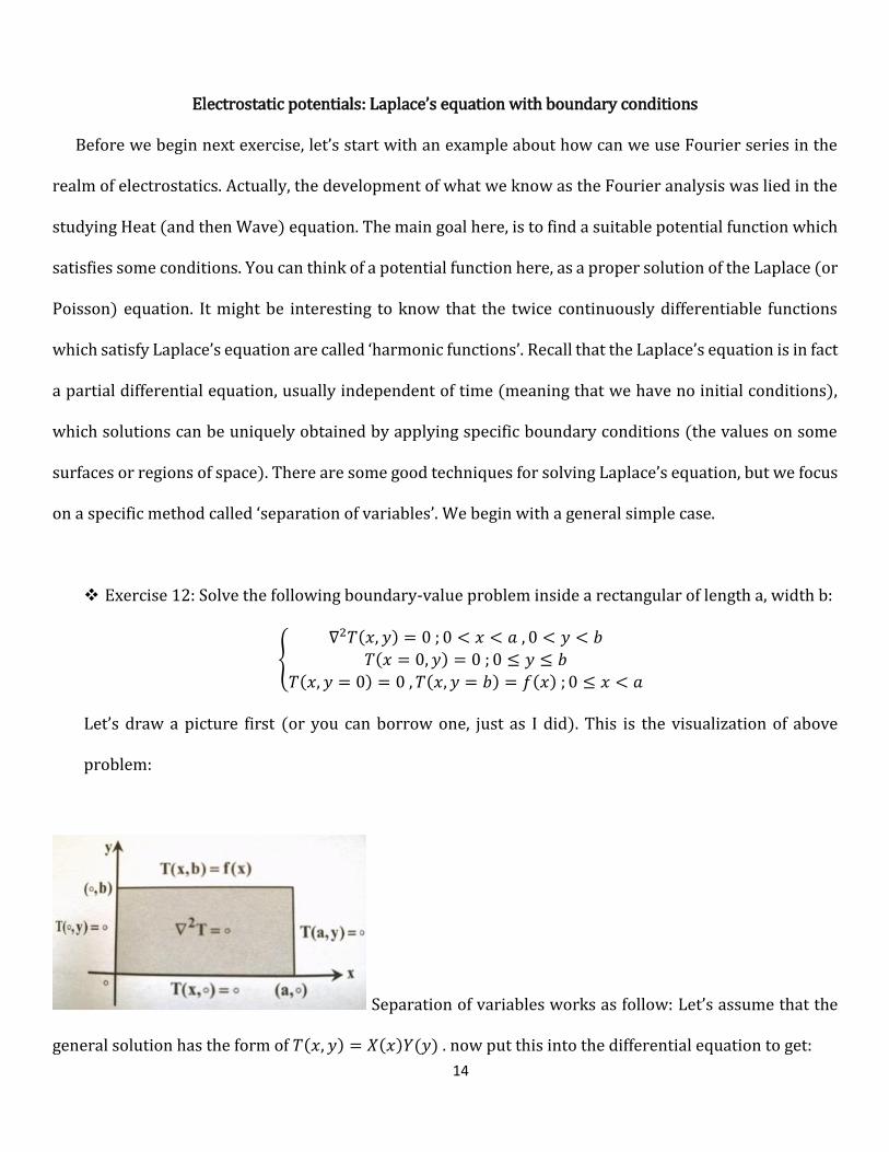
Exercise 12: Solve the following boundary-value problem inside a rectangular of length a, width b:

{

∇2𝑇(𝑥, 𝑦) = 0 ; 0 < 𝑥 < 𝑎 , 0 < 𝑦 < 𝑏

𝑇(𝑥 = 0, 𝑦) = 0 ; 0 ≤ 𝑦 ≤ 𝑏

𝑇(𝑥, 𝑦 = 0) = 0 , 𝑇(𝑥, 𝑦 = 𝑏) = 𝑓(𝑥) ; 0 ≤ 𝑥 < 𝑎

Let’s draw a picture first (or you can borrow one, just as I did). This is the visualization of above

problem:

Separation of variables works as follow: Let’s assume that the

general solution has the form of 𝑇(𝑥, 𝑦) = 𝑋(𝑥)𝑌(𝑦) . now put this into the differential equation to get:

15

𝑋′′(𝑥)

𝑋(𝑥)+

𝑌′′(𝑦)

𝑌(𝑦)= 0 . let’s assume that the two fractions have the same value, different in the sign so that they

could cancel each other to zero: 𝑋′′(𝑥)

𝑋(𝑥)= −𝜆 ,

𝑌′′(𝑦)

𝑌(𝑦)= 𝜆 . now applying the boundary conditions, we get:

𝑇(0, 𝑦) = 𝑋(0)𝑌(𝑦) = 0 → 𝑋(0) = 0 ; 𝑇(𝑎, 𝑦) = 𝑋(𝑎)𝑌(𝑦) = 0 → 𝑋(𝑎) = 0 . therefore for x, we have the

following differential equation: {𝑋′′(𝑥) + 𝜆𝑋(𝑥) = 0

𝑋(0) = 𝑋(𝑎) = 0 . let 𝜆 = 𝜔2, which gives us the familiar solution:

𝑋(𝑥) = 𝐴𝑐𝑜𝑠(𝜔𝑥) + 𝐵𝑠𝑖𝑛(𝜔𝑥) . by applying the conditions, we get 𝑋(0) = 𝐴 = 0, 𝑋(𝑎) = 𝐵𝑠𝑖𝑛(𝜔𝑎) = 0 →

𝜔 =𝑛𝜋

𝑎≡ 𝜔𝑛 → 𝑋𝑛(𝑥) = 𝐵𝑛 sin (

𝑛𝜋𝑥

𝑎) . Now for the y, given the obtained 𝜔, we have: 𝑌′′(𝑦) −

(𝑛𝜋

𝑎)

2

𝑌(𝑦) = 0 → 𝑌𝑛(𝑦) = 𝐶𝑛 cosh (𝑛𝜋𝑦

𝑎) + 𝐷𝑛 sinh (

𝑛𝜋𝑦

𝑎) . again by conditions, we get 𝐶𝑛 = 0 → 𝑌𝑛(𝑦) =

𝐷𝑛 sinh (𝑛𝜋𝑦

𝑎) . multiplying the results, the general form of the solution will be 𝑇𝑛(𝑥, 𝑦) = 𝑋𝑛(𝑥)𝑌𝑛(𝑦) =

𝐵𝑛𝐷𝑛 sinh (𝑛𝜋𝑦

𝑎) sin (

𝑛𝜋𝑥

𝑎). Now let’s combine the coefficients into one: 𝐸𝑛 ≡ 𝐵𝑛𝐷𝑛 . then for all values of n

we have to sum the solution over n, therefore: 𝑇𝑛(𝑥, 𝑦) = ∑ 𝐸𝑛 sinh (𝑛𝜋𝑦

𝑎) sin (

𝑛𝜋𝑥

𝑎) .∞

𝑛=1 Now let’s apply the

final boundary condition 𝑇(𝑥, 𝑦 = 𝑏) = 𝑓(𝑥) → 𝑓(𝑥) = ∑ 𝐸𝑛 sinh (𝑛𝜋𝑏

𝑎) sin (

𝑛𝜋𝑥

𝑎) .∞

𝑛=1 Now do you see any

familiar stuff here? You’re right! 𝑓 has expanded as the sine Fourier series with the coefficients of 𝑏𝑛 =

𝐸𝑛 sinh (𝑛𝜋𝑏

𝑎) . you do remember that for the Fourier coefficients we had 𝑏𝑛 =

2

𝐿∫ 𝑓(𝑥) sin (

𝑛𝜋𝑥

𝐿) 𝑑𝑥 →

𝐿

0

Here 𝐿 = 𝑎 ⟹ 𝐸𝑛 sinh (𝑛𝜋𝑏

𝑎) =

2

𝑎∫ 𝑓(𝑥) sin (

𝑛𝜋𝑥

𝑎) 𝑑𝑥 → 𝐸𝑛 =

2

asinh (𝑛𝜋𝑏

𝑎)

∫ 𝑓(𝑥) sin (𝑛𝜋𝑥

𝑎) 𝑑𝑥 .

𝑎

0

𝑎

0

Voila! You can see that if the explicit form of 𝑓(𝑥) is given, then you can compute 𝐸𝑛 , ergo finding the

explicit form for 𝑇𝑛(𝑥, 𝑦), i.e. the solution of the desired equation. ∎

Whoa! What a lengthy answer for such a short problem! But don’t worry, you’ll get used to it by more

practice. Now let’s get physical by the next exercise.

16

[Arfken 19.2.11]: The treatment for this problem is same as the previous one, except that the

geometry has changed and we need to work in cylindrical coordinates. The general form of the

Laplacian in cylindrical coordinates is ∇2𝜙(𝑟, 𝜑, 𝑧) =1

𝑟

𝜕

𝜕𝑟(𝑟

𝜕𝜙(𝑟,𝜑,𝑧)

𝜕𝑟) +

1

𝑟2

𝜕2𝜙(𝑟,𝜑,𝑧)

𝜕𝜑2 +𝜕2𝜙(𝑟,𝜑,𝑧)

𝜕𝑧2 . by

separation method, we have 𝜙(𝑟, 𝜑, 𝑧) = 𝑅(𝑟)𝐹(𝜑)𝑍(𝑧) . substituting this into Laplace’s equation we

get ∇2𝜙(𝑟, 𝜑, 𝑧) = 0 =1

𝑅

𝑑2𝑅

𝑑𝑟2 +1

𝑟𝑅

𝑑𝑅

𝑑𝑟+

1

𝑟2𝐹

𝑑2𝐹

𝑑𝜑2 +1

𝑍

𝑑2𝑍

𝑑𝑧2 . let’s put 1

𝑍

𝑑2𝑍

𝑑𝑧2 = 𝑘2 (𝑎 𝑐𝑜𝑛𝑠𝑡𝑎𝑛𝑡). This gives us

the equation for Z: 𝑑2𝑍

𝑑𝑧2− 𝑘2𝑍(𝑧) = 0 . now returning to the main equation, we’ll see that

𝑟2

𝑅

𝑑2𝑅

𝑑𝑟2+

𝑟

𝑅

𝑑𝑅

𝑑𝑟+

𝑘2𝑟2 = −1

𝐹

𝑑2𝐹

𝑑𝜑2 . now let’s put -

1

𝐹

𝑑2𝐹

𝑑𝜑2= 𝑚2 →

𝑑2𝐹

𝑑𝜑2+ 𝑚2𝐹(𝜑) = 0 . therefore

𝑑2𝑅

𝑑𝑟2+

1

𝑟

𝑑𝑅

𝑑𝑟+ (𝑘2 −

𝑚2

𝑟2) 𝑅 =

0 . the solutions for Z, F are easy: 𝑍(𝑧) = 𝑒±𝑘𝑧 , 𝐹(𝜑) = 𝑒±𝑖𝑚𝜑 . the tough one is for R. interestingly

there’s a solution for it: if we set 𝑥 = 𝑘𝑟 → 𝑑2𝑅

𝑑𝑥2 +1

𝑥

𝑑𝑅

𝑑𝑥+ (1 −

𝑚2

𝑥2 ) 𝑅 = 0 , which is the Bessel equation

and the solutions are called Bessel functions of order m (which we are not going to elaborate here. If

you’re interested, you can find the details in any book covering the special functions. For example, see

Alan Jeffrey & Hui-Hui Dai‘s Handbook of Mathematical Formulas and Integrals). In here, we simplify

our approach by assuming that potential is symmetric in z, i.e. 𝜙(𝑟, 𝜑, 𝑧) ≡ 𝜙(𝑟, 𝜑) = 𝑅(𝑟)𝐹(𝜑) .

therefore the radial equation takes the form of 𝑟2𝑅′′(𝑟) + 𝑟𝑅′(𝑟) − 𝑘2𝑅(𝑟) = 0 which has the power

series solution of the form 𝑅(𝑟) = ∑ 𝑎𝑛𝑟𝑛 .∞𝑛=1 since we can rewrite the solutions of 𝐹(𝜑) as 𝐹(𝜑) =

𝐴𝑚 cos(𝑚𝜑) + 𝐵𝑚 sin(𝑚𝜑) , therefore for the interior of the cylinder we can write the general solution

as 𝜙(𝑟, 𝜑) = 𝐴0 + ∑ 𝑟𝑚[∞𝑚=1 𝐴𝑚 cos(𝑚𝜑) + 𝐵𝑚 sin(𝑚𝜑)] . note that for the exterior region (𝑟 > 𝑅) we

should include the negative values of m instead. Now let’s dismiss 𝐴0 for now (no free charge). Now

since we have 𝜙(𝑟, 𝜑) = −𝜙(𝑟, −𝜑) , this means that solution should not be dependent on Cosine terms

(Cosine is even function), therefore 𝜙(𝑟, 𝜑) = ∑ 𝑟𝑚𝐵𝑚 sin(𝑚𝜑)∞𝑚=1 . now due to our boundary

conditions, 𝜙(𝑟 = 𝑎, 𝜑) = ±𝑉 = ∑ 𝑎𝑚𝐵𝑚 sin(𝑚𝜑)∞𝑚=1 → 𝑎𝑚𝐵𝑚 =

1

𝜋∫ ±𝑉𝑠𝑖𝑛(𝑚𝜑)𝑑𝜑 =

2𝜋

0

17

𝑉

𝜋{∫ 𝑠𝑖𝑛(𝑚𝜑)𝑑𝜑 − ∫ 𝑠𝑖𝑛(𝑚𝜑)𝑑𝜑

2𝜋

𝜋=

4𝑉

𝑚𝜋 (𝑚 𝑖𝑠 𝑜𝑑𝑑) → 𝜙(𝑟, 𝜑) =

4𝑉

𝜋∑ (

𝑟

𝑎)𝑚 sin (𝑚𝜑)

𝑚 ,∞

𝑚=1𝜋

0 for odd m, or

equivalently 𝜙(𝑟, 𝜑) =4𝑉

𝜋∑ (

𝑟

𝑎)2𝑚+1 sin (2𝑚+1)𝜑

2𝑚+1 ∎∞

𝑚=1

☠ [Arfken 19.2.12]: up to you.

[Arfken 19.2.19]: I will just give you some insights on this one and I’ll let you handle the details on

your own. First, consider the separation of variables method and separate the general solution

into the product of spatial and temporal functions as 𝑦(𝑥, 𝑡) = 𝑋(𝑥)𝑇(𝑡) , and proceed with the

method. Then solve each equation and obtain the general solution. Then apply the boundary and

initial conditions. “clamped” means that the boundary condition has the form of Dirichlet’s, i.e.

𝑢(0, 𝑡) = 𝑢(𝐿, 𝑡) = 0 Then use what you know about the Fourier series to obtain the proper

coefficients. At last you will be able to write down the solution of the wave equation in terms of

the infinite series. You might during the calculations need the following expansion of Dirac delta

function: 𝛿(𝑥 − 𝑎) =2

𝐿∑ sin (

𝑛𝜋𝑎

𝐿) sin (

𝑛𝜋𝑥

𝐿) ,∞

𝑛=1 defined in half interval of (0, 𝐿) ∎

! Note that there is an easier way to deal with wave equation, without getting headaches, which is

the Fourier transform. Don’t worry, we shall meet her next time soon.

☠ [Arfken 19.2.20] & [Arfken 19.2.21]: Do it yourself. You’re on your own! [You need to hand in just

one of them, not both]

18

Epilogue

Well guys, I wish our little journey were fun for you. I could have included more exercises but

unfortunately my time was limited. I hope we meet again, this time on the subject of Fourier and

Laplace transform, two gorgeous tools of doing magic. At the end, let me say something about life

(I’m not gonna preach you, relax). Life is more pleasant if you include sometimes some literature

(among other things, of course) into your everyday rides in physics and mathematics. That’s why I

would like to end this note with a quote from Absalom! Absalom! by the great William Faulkner. I

hope you enjoy it:

“You get born and you try this and you don't know why only you keep on trying it and you are born at the

same time with a lot of other people, all mixed up with them, like trying to, having to, move your arms and

legs with strings only the same strings are hitched to all the other arms and legs and the others all trying

and they don't know why either except that the strings are all in one another's way like five or six people

all trying to make a rug on the same loom only each one wants to weave his own pattern into the rug; and

it can't matter, you know that, or the Ones that set up the loom would have arranged things a little better,

and yet it must matter because you keep on trying or having to keep on trying and then all of a sudden it's

all over and all you have left is a block of stone with scratches on it provided there was someone to

remember to have the marble scratched and set up or had time to, and it rains on it and then sun shines on

it and after a while they don't even remember the name and what the scratches were trying to tell, and it

doesn't matter. And so maybe if you could go to someone, the stranger the better, and give them something-

a scrap of paper-something, anything, it not to mean anything in itself and them not even to read it or keep

it, not even bother to throw it away or destroy it, at least it would be something just because it would have

happened, be remembered even if only from passing from one hand to another, one mind to another, and

it would be at least a scratch, something, something that might make a mark on something that was once

for the reason that it can die someday, while the block of stone can't be is because it never can become was

because it can't ever die or perish...”

19

[This Page Is Intentionally Left Blank]

ArfKen_Ch19-9780123846549.tex

19.1 General Properties 945

Exercises

19.1.1 A function f (x) (quadratically integrable) is to be represented by a finite Fourier series.A convenient measure of the accuracy of the series is given by the integrated square ofthe deviation,

1p =

2π∫0

[f (x)−

a0

2−

p∑n=1

(an cos nx + bn sin nx)

]2

dx .

Show that the requirement that 1p be minimized, that is,

∂1p

∂an= 0,

∂1p

∂bn= 0,

for all n, leads to choosing an and bn as given in Eqs. (19.2) and (19.3).

Note. Your coefficients an and bn are independent of p. This independence is a conse-quence of orthogonality and would not hold if we expanded f (x) in a power series.

19.1.2 In the analysis of a complex waveform (ocean tides, earthquakes, musical tones, etc.),it might be more convenient to have the Fourier series written as

f (x)=a0

2+

∞∑n=1

αn cos(nx − θn).

Show that this is equivalent to Eq. (19.1) with

an = αn cos θn, α2n = a2

n + b2n,

bn = αn sin θn, tan θn = bn/an .

Note. The coefficients α2n as a function of n define what is called the power spectrum.

The importance of α2n lies in their invariance under a shift in the phase θn .

19.1.3 A function f (x) is expanded in an exponential Fourier series

f (x)=∞∑

n=−∞

cneinx .

If f (x) is real, f (x)= f ∗(x), what restriction is imposed on the coefficients cn?

19.1.4 Assuming that∫ π−π[ f (x)]2dx is finite, show that

limm→∞

am = 0, limm→∞

bm = 0.

Hint. Integrate [ f (x) − sn(x)]2, where sn(x) is the nth partial sum, and use Bessel’sinequality (Section 5.1). For our finite interval the assumption that f (x) is square inte-grable (

∫ π−π| f (x)|2 dx is finite) implies that

∫ π−π| f (x)| dx is also finite. The converse

does not hold.

ArfKen_Ch19-9780123846549.tex

946 Chapter 19 Fourier Series

3ππ−π

2π

2π−

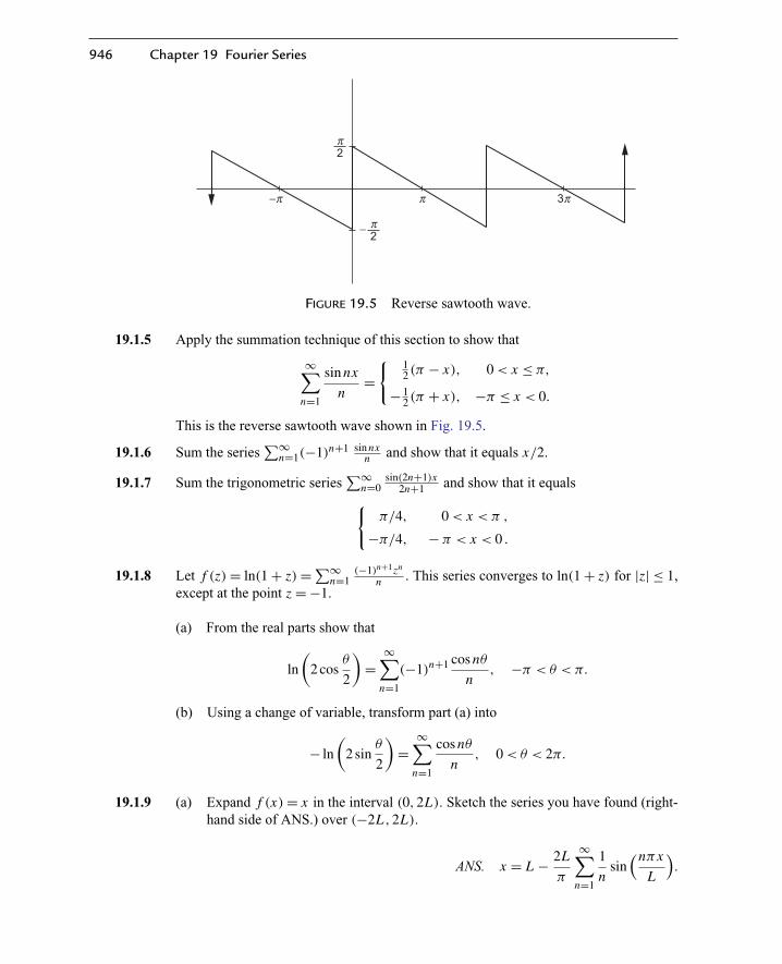
FIGURE 19.5 Reverse sawtooth wave.

19.1.5 Apply the summation technique of this section to show that

∞∑n=1

sin nx

n=

{ 12 (π − x), 0< x ≤ π,

−12 (π + x), −π ≤ x < 0.

This is the reverse sawtooth wave shown in Fig. 19.5.

19.1.6 Sum the series∑∞

n=1(−1)n+1 sin nxn and show that it equals x/2.

19.1.7 Sum the trigonometric series∑∞

n=0sin(2n+1)x

2n+1 and show that it equals{π/4, 0< x < π ,

−π/4, − π < x < 0 .

19.1.8 Let f (z)= ln(1+ z)=∑∞

n=1(−1)n+1zn

n . This series converges to ln(1+ z) for |z| ≤ 1,except at the point z =−1.

(a) From the real parts show that

ln

(2 cos

θ

2

)=

∞∑n=1

(−1)n+1 cos nθ

n, −π < θ < π.

(b) Using a change of variable, transform part (a) into

− ln

(2 sin

θ

2

)=

∞∑n=1

cos nθ

n, 0< θ < 2π.

19.1.9 (a) Expand f (x)= x in the interval (0,2L). Sketch the series you have found (right-hand side of ANS.) over (−2L ,2L).

ANS. x = L −2L

π

∞∑n=1

1

nsin(nπx

L

).

ArfKen_Ch19-9780123846549.tex

19.1 General Properties 947

(b) Expand f (x)= x as a sine series in the half interval (0, L). Sketch the series youhave found (right-hand side of Ans.) over (−2L ,2L).

ANS. x =4L

π

∞∑n=0

1

2n + 1sin

((2n + 1)πx

L

).

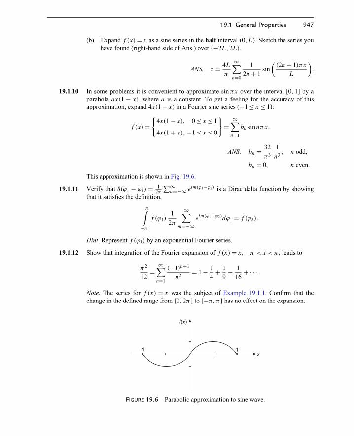
19.1.10 In some problems it is convenient to approximate sinπx over the interval [0,1] by aparabola ax(1 − x), where a is a constant. To get a feeling for the accuracy of thisapproximation, expand 4x(1− x) in a Fourier sine series (−1≤ x ≤ 1):

f (x)=

{4x(1− x), 0≤ x ≤ 1

4x(1+ x), −1≤ x ≤ 0

}=

∞∑n=1

bn sin nπx .

ANS. bn =32

π3

1

n3 , n odd,

bn = 0, n even.

This approximation is shown in Fig. 19.6.

19.1.11 Verify that δ(ϕ1 − ϕ2) =1

2π

∑∞

m=−∞ eim(ϕ1−ϕ2) is a Dirac delta function by showingthat it satisfies the definition,

π∫−π

f (ϕ1)1

2π

∞∑m=−∞

eim(ϕ1−ϕ2)dϕ1 = f (ϕ2).

Hint. Represent f (ϕ1) by an exponential Fourier series.

19.1.12 Show that integration of the Fourier expansion of f (x)= x , −π < x < π , leads to

π2

12=

∞∑n=1

(−1)n+1

n2 = 1−1

4+

1

9−

1

16+ · · · .

Note. The series for f (x) = x was the subject of Example 19.1.1. Confirm that thechange in the defined range from [0,2π ] to [−π,π] has no effect on the expansion.

f(x)

x1−1

FIGURE 19.6 Parabolic approximation to sine wave.

ArfKen_Ch19-9780123846549.tex


19.1.13 (a) Assuming that the Fourier expansion of f (x) is uniformly convergent, show that

1

π

π∫−π

[f (x)

] 2dx =

a20

2+

∞∑n=1

(a2n + b2

n).

This is Parseval’s identity. Note that it is a completeness relation for the Fourierexpansion.

(b) Given x2=π2

3+ 4

∞∑n=1

(−1)n cos nx

n2 , −π ≤ x ≤ π,

apply Parseval’s identity to obtain ζ(4) in closed form.

(c) The condition of uniform convergence is not necessary. Show this by applying theParseval identity to the square wave

f (x)=

{−1, −π < x < 0

1, 0< x < π

=4

π

∞∑n=1

sin(2n − 1)x

2n − 1.

19.1.14 Given

ϕ1(x)≡∞∑

n=1

sin nx

n=

−

1

2(π + x), −π ≤ x < 0,

1

2(π − x), 0< x ≤ π,

show by integrating that

ϕ2(x)≡∞∑

n=1

cos nx

n2 =

1

4(π + x)2 −

π2

12, −π ≤ x ≤ 0,

1

4(π − x)2 −

π2

12, 0≤ x ≤ π.

19.1.15 Given

ψ2s(x)=∞∑

n=1

sin nx

n2s, ψ2s+1(x)=

∞∑n=1

cos nx

n2s+1 ,

develop the following recurrence relations:

(a) ψ2s(x)=

x∫0

ψ2s−1(x)dx ,

(b) ψ2s+1(x)= ζ(2s + 1)−

x∫0

ψ2s(x)dx .

ArfKen_Ch19-9780123846549.tex

19.2 Applications of Fourier Series 949

Note. The functions ψs(x) and ϕs(x) of this and the preceding exercise are known asClausen functions. In theory they may be used to improve the rate of convergence ofa Fourier series. As is often the case, there is the question of how much analytical workwe do and how much arithmetic work we demand that a computer do. As computersbecome steadily more powerful, the balance progressively shifts so that we are doingless and demanding that computers do more.

19.1.16 Show that f (x)=∑∞

n=1cos nxn+1 may be written as

f (x)=ψ1(x)− ϕ2(x)+∞∑

n=1

cos nx

n2(n + 1),

where ψ1(x) and ϕ2(x) are the Clausen functions defined in Exercises 19.1.14 and19.1.15.

19.2 APPLICATIONS OF FOURIER SERIES

We present in this section two typical problems and a short table of useful Fourier series,followed by a substantial number of exercises that illustrate some of the techniques thatarise in applications.

Example 19.2.1 SQUARE WAVE

One application of Fourier series, the analysis of a “square” wave (Fig. 19.7) in terms of itsFourier components, occurs in electronic circuits designed to handle sharply rising pulses.Suppose that our wave is defined by

f (x)= 0, −π < x < 0,(19.25)

f (x)= h, 0< x < π.

f (x)

x

h

π−3π 3π−2π 2π−π

FIGURE 19.7 Square wave.

ArfKen_Ch19-9780123846549.tex


Table 19.1 Some Fourier Series Used in This Text

Fourier Series Reference

1.∞∑

n=1

sin nx

n=

{−

12 (π + x), −π ≤ x < 012 (π − x), 0≤ x < π

Exercise 19.1.5Exercise 19.2.8

2.∞∑

n=1

(−1)n+1 sin nx

n=

x

2, −π < x < π

Exercise 19.1.6

Exercise 19.2.7

3.∞∑

n=0

sin(2n + 1)x

2n + 1=

{−π/4, −π < x < 0

+π/4, 0< x < π

Exercise 19.1.7

Eq. (19.26)

4.∞∑

n=1

cos nx

n=− ln

[2 sin

(|x |

2

)], −π < x < π

Exercise 19.1.8(b)

Eq. (19.24)

5.∞∑

n=1

(−1)ncos nx

n=− ln

[2 cos

( x

2

)], −π < x < π Exercise 19.1.8(a)

6.∞∑

n=0

cos(2n + 1)x

2n + 1=

1

2ln

[cot|x |

2

], −π < x < π Exercise 19.2.5

Exercises

19.2.1 Transform the Fourier expansion of a square wave, Eq. (19.26), into a power series.Show that the coefficients of x1 form a divergent series. Repeat for the coefficientsof x3.

Note. A power series cannot handle a discontinuity. These infinite coefficients are theresult of attempting to beat this basic limitation on power series.

19.2.2 Derive the Fourier series expansion of the Dirac delta function δ(x) in the interval−π < x < π .

(a) What significance can be attached to the constant term?

(b) In what region is this representation valid?

(c) With the identity

N∑n=1

cos nx =sin(N x/2)

sin(x/2)cos

[(N +

1

2

)x

2

],

show that your Fourier representation of δ(x) is consistent with Eq. (5.27).

19.2.3 Expand δ(x − t) in a Fourier series. Compare your result with the bilinear form ofEq. (5.27).

ArfKen_Ch19-9780123846549.tex


ANS. δ(x − t)=1

2π+

1

π

∞∑n=1

(cos nx cos nt + sin nx sin nt)

=1

2π+

1

π

∞∑n=1

cos n(x − t).

19.2.4 Show that integrating the Fourier expansion of the Dirac delta function (Exercise 19.2.2)leads to the Fourier representation of the square wave, Eq. (19.26), with h = 1.

Note. Integrating the constant term (1/2π) leads to a term x/2π . What are you goingto do with this?

19.2.5 Starting from the Fourier series given as lines 4 and 5 of Table 19.1, show that:

∞∑n=0

cos(2n + 1)x

2n + 1=

1

2ln

[cot|x |

2

].

19.2.6 Develop the Fourier series representation of

f (t)=

{0, −π ≤ ωt ≤ 0,

sinωt, 0≤ ωt ≤ π.

This is the output of a simple half-wave rectifier. It is also an approximation of the solarthermal effect that produces “tides” in the atmosphere.

ANS. f (t)=1

π+

1

2sinωt −

2

π

∞∑n=2,4,6,...

cos nωt

n2 − 1.

19.2.7 A sawtooth wave is given by

f (x)= x, −π < x < π.

Show that

f (x)= 2∞∑

n=1

(−1)n+1

nsin nx .

19.2.8 A different sawtooth wave is described by

f (x)=

{−

12 (π + x), −π ≤ x < 0

+12 (π − x), 0< x ≤ π.

Show that f (x)=∞∑

n=1

(sin nx/n).

19.2.9 A triangular wave (Fig. 19.4) is represented by

f (x)=

{x, 0< x < π

−x, −π < x < 0.

ArfKen_Ch19-9780123846549.tex


Represent f (x) by a Fourier series.

ANS. f (x)=π

2−

4

π

∑n=1,3,5,...

cos nx

n2 .

19.2.10 Expand

f (x)=

{1, x2 < x2

0

0, x2 > x20

in the interval [−π,π].

Note. This variable-width square wave is of some importance in electronic music.

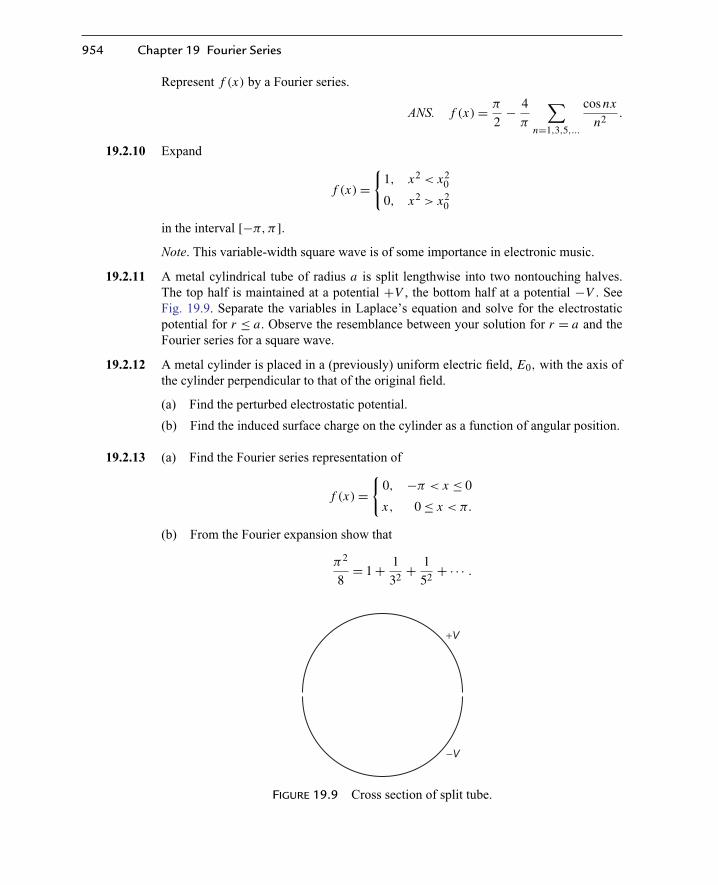
19.2.11 A metal cylindrical tube of radius a is split lengthwise into two nontouching halves.The top half is maintained at a potential +V , the bottom half at a potential −V . SeeFig. 19.9. Separate the variables in Laplace’s equation and solve for the electrostaticpotential for r ≤ a. Observe the resemblance between your solution for r = a and theFourier series for a square wave.

19.2.12 A metal cylinder is placed in a (previously) uniform electric field, E0, with the axis ofthe cylinder perpendicular to that of the original field.

(a) Find the perturbed electrostatic potential.

(b) Find the induced surface charge on the cylinder as a function of angular position.

19.2.13 (a) Find the Fourier series representation of

f (x)=

{0, −π < x ≤ 0

x, 0≤ x < π.

(b) From the Fourier expansion show that

π2

8= 1+

1

32 +1

52 + · · · .

+V

−V

FIGURE 19.9 Cross section of split tube.

ArfKen_Ch19-9780123846549.tex


δn(x)

n

−π π− 12n

12n

x

FIGURE 19.10 Rectangular pulse.

19.2.14 Integrate the Fourier expansion of the unit step function

f (x)=

{0, −π < x < 0

1, 0< x < π.

Show that your integrated series agrees with Exercise 19.2.13.

19.2.15 In the interval (−π,π), δn(x)=

{n, |x |< 1/2n,

0, |x |> 1/2n.

This wave form is the pulse shown in Fig. 19.10.

(a) Expand δn(x) as a Fourier cosine series.

(b) Show that your Fourier series agrees with a Fourier expansion of δ(x) in the limitas n→∞.

19.2.16 Confirm the delta function nature of your Fourier series of Exercise 19.2.15 by showingthat for any f (x) that is finite in the interval [−π,π] and continuous at x = 0,

π∫−π

f (x) [Fourier expansion of δ∞(x)] dx = f (0).

19.2.17 (a) Show that the Dirac delta function δ(x − a), expanded in a Fourier sine series inthe half-interval (0, L) (0< a < L) is given by

δ(x − a)=2

L

∞∑n=1

sin(nπa

L

)sin(nπx

L

).

Note that this series actually describes −δ(x + a) + δ(x − a) in the interval(−L , L).

(b) By integrating both sides of the preceding equation from 0 to x , show that thecosine expansion of the square wave

f (x)=

{0, 0≤ x < a

1, a < x < L ,

ArfKen_Ch19-9780123846549.tex


is

f (x)=2

π

∞∑n=1

1

nsin(nπa

L

)−

2

π

∞∑n=1

1

nsin(nπa

L

)cos

(nπx

L

),

for 0≤ x < L .

(c) Show that the term2

π

∞∑n=1

1

nsin(nπa

L

)is the average of f (x) on (0, L).

19.2.18 Verify the Fourier cosine expansion of the square wave, Exercise 19.2.17(b), by directcalculation of the Fourier coefficients.

19.2.19 (a) A string is clamped at both ends x = 0 and x = L . Assuming small-amplitudevibrations, we find that the amplitude y(x, t) satisfies the wave equation

∂2 y

∂x2 =1

v2

∂2 y

∂t2 .

Here v is the wave velocity. The string is set in vibration by a sharp blow at x = a.Hence we have

y(x,0)= 0,∂y(x, t)

∂t= Lv0δ(x − a) at t = 0.

The constant L is included to compensate for the dimensions (inverse length) ofδ(x − a). With δ(x − a) given by Exercise 19.2.17(a), solve the wave equationsubject to these initial conditions.

ANS. y(x, t)=2v0L

πv

∞∑n=1

1

nsin

nπa

Lsin

nπx

Lsin

nπvt

L.

(b) Show that the transverse velocity of the string ∂y(x, t)/∂t is given by

∂y(x, t)

∂t= 2v0

∞∑n=1

sinnπa

Lsin

nπx

Lcos

nπvt

L.

19.2.20 A string, clamped at x = 0 and at x = L , is vibrating freely. Its motion is described bythe wave equation

∂2u(x, t)

∂t2 = v2 ∂2u(x, t)

∂x2 .

Assume a Fourier expansion of the form

u(x, t)=∞∑

n=1

bn(t) sinnπx

L

and determine the coefficients bn(t). The initial conditions are

u(x,0)= f (x) and∂

∂tu(x,0)= g(x).

ArfKen_Ch19-9780123846549.tex

19.3 Gibbs Phenomenon 957

Note. This is only half the conventional Fourier orthogonality integral interval. How-ever, as long as only the sines are included here, the Sturm-Liouville boundary condi-tions are still satisfied and the functions are orthogonal.

ANS. bn(t)= An cosnπvt

L+ Bn sin

nπvt

L,

An =2

L

L∫0

f (x) sinnπx

Ldx, Bn =

2

nπv

L∫0

g(x) sinnπx

Ldx .

19.2.21 (a) Let us continue the vibrating string problem in Exercise 19.2.20. We assume nowthat the presence of a resisting medium will damp the vibrations according to theequation

∂2u(x, t)

∂t2 = v2 ∂2u(x, t)

∂x2 − k∂u(x, t)

∂t.

Introduce a Fourier expansion

u(x, t)=∞∑

n=1

bn(t) sinnπx

L

and again determine the coefficients bn(t). Take the initial and boundary condi-tions to be the same as in Exercise 19.2.20. Assume the damping to be small.

(b) Repeat, but assume the damping to be large.

ANS.

(a) bn(t)= e−kt/2[An cosωn t + Bn sinωn t], ω2

n =

(nπv

L

)−

(k

2

)2

> 0,

An =2

L

L∫0

f (x) sinnπx

Ldx, Bn =

2

ωn L

L∫0

g(x) sinnπx

Ldx +

k

2ωnAn .

(b) bn(t)= e−kt/2[An coshσn t + Bn sinhσn t], σ 2

n =

(k

2

)2

−

(nπv

L

)2> 0,

An =2

L

L∫0

f (x) sinnπx

Ldx, Bn =

2

σn L

L∫0

g(x) sinnπx

Ldx +

k

2σnAn .

19.3 GIBBS PHENOMENON

The Gibbs phenomenon is an overshoot, a peculiarity of the Fourier series and other eigen-function series at a simple discontinuity. An example is seen in Fig. 19.2.

Partial Summation of Fourier Series

To better understand the Gibbs phenomenon we examine methods for the partial summa-tion of Fourier series. This procedure is unlikely to lead to convenient solutions of practical

a companion to fourier series - دانشگاه...

Documents