A Common Value Auction with State Dependent

Participation∗

Stephan Lauermann† Asher Wolinsky‡

April 15, 2016

We study a common value, first-price auction in which the number of bidders is

endogenous: the seller (auctioneer) knows the value and solicits bidders at a cost.

The number of bidders, which is unobservable, may thus depend on the true value.

Therefore, being solicited already conveys information. This “solicitation effect”may

soften competition and may impede information aggregation. Under certain condi-

tions, there is an equilibrium in which the auctioneer solicits many bidders, yet the

resulting price is not competitive and it fails to aggregate any information. This stands

in contrast to the familiar outcomes of standard auctions.

This paper analyzes a common value, first-price auction with the novel feature that the

number of bidders may depend on the value. Specifically, there is a single good and two

states, ` and h, with the common value of the good, vω, ω = `, h, satisfying vh > v`. In

state ω there are nω bidders, who receive conditionally independent signals, but do not

observe ω or nω.

We explore the bidding equilibria of this game. One of the main insights is that, owing

to the state dependent participation, competition between bidders can be softened to the

point where bidders with high signals are pooling on a common bid (atom) below the

ex-ante expected value. This means that, when there are many bidders, the winning bid

is essentially independent of the state and possibly non-competitive. This is interesting

∗The authors gratefully acknowledge support from the National Science Foundation under Grants SES-1123595 and SES-1061831. Qinggong Wu, Au Pak, Deniz Kattwinkel, and Guannan Luo provided excellentresearch assistance.†University of Bonn, Department of Economics, s.lauermann@uni-bonn.de.‡Northwestern University, Department of Economics, a-wolinsky@northwestern.edu.

1

and somewhat surprising from the perspective of auction analysis. But, perhaps more

importantly, this reduced competitiveness has implications for the extent of information

aggregation by markets with adverse selection.

To understand this insight, recall that, in an ordinary common value auction, winning

at a lower bid reflects more negatively on the value of the object than winning at a

higher bid. Consequently, partially informed bidders try to evade adverse selection by

bidding more aggressively and in the process inject their information into the price. For

this reason, an ordinary auction with many bidders is both nearly competitive and may

aggregate the information well. In contrast, with state dependent participation, more

aggressive bidding might involve more severe adverse selection. If there are suffi ciently

more bidders in state ` than in state h, just being included in the auction already involves

a “participation curse” that depresses the expected value estimate held by a bidder. A

bidder who overbids everybody else, would bear the full strength of this “curse.” But

a winning bid from the “middle” of the winning bid distribution would give rise to a

“middle winner’s blessing” that partly offsets the “participation curse.” The reason is

that more bidders are likely to bid near or above the “middle” in state ` and therefore,

conditional on winning, the probability of state h is higher than its interim probability.

This induces bidders to escape the “participation curse“ by aiming at a “middling”bid.

They are thus driven away from overbidding and towards more pooling. Consequently,

both the competition and the incorporation of information into prices are dampened.

Our main characterization result concerns the general form of the bidding equilibrium,

when there are many bidders in each state. To explain it, let Gω denote the c.d.f. of the

(conditionally independent) signals received by bidders in state ω, with support on [x, x̄]

and density gω. Assume that the likelihood ratiogh(x)g`(x) is monotonically increasing so that

x̄ is the most favorable signal for h. When n` and nh are suffi ciently large, the general

form of bidding equilibria is determined by the magnitude of gh(x̄)g`(x̄)

nhn`. If this ratio is

below 1, then any bidding equilibrium is necessarily of the pooling type mentioned above.

If this ratio is above 1, then any bidding equilibrium is necessarily of a separating type,

resembling the equilibrium of an ordinary common value auction with no significant atoms

in the winning bid distribution and with a higher expected winning bid in state h than in

`.

State dependent participation may arise for a number of reasons. This paper focuses on

a straightforward reason– costly solicitation of bidders by an informed seller, who knows

ω, and invites nω bidders to participate.1 It is natural to wonder whether an equilibrium of

the full game with a strategic solicitation decision rules out any of the patterns described

1 In Murto and Välimäki (2015) state dependent participation arises because the bidders make costlyentry decisions after receiving their signals; in Atakan and Ekmekci (2015) bidders’entry decisions differacross states due to differences in the value of outside options. A range of behavioral considerations mighthave a similar effect as well.

2

above. Indeed, another insight of this paper is that a non-competitive atom of the type

discussed above may arise in an equilibrium of the full game.2

Let us point out this paper’s main contributions. From the conceptual perspective,

one contribution is the idea of considering an auction with state dependent participation.

As mentioned before, this could arise for a variety of reasons and, while there might be

some differences among different scenarios of this type, the main considerations should be

similar. Therefore, shining the light on price formation in the presence of this consideration

is interesting in it’s own right, independently of the specifics of an underlying process that

determines the participation.

From the substantive perspective, two of the paper’s main contributions are, first, the

introduction of a new model that seems relevant for numerous economically interesting

situations and, second, obtaining insights with obvious implications. The most distinct of

those insights are the potential emergence of an atom in the winning bid distribution and

the associated failures of competitiveness and information aggregation. Let us elaborate

on these two contributions.

Viewed narrowly as a model of a single auction with bidder solicitation, it captures

a hitherto neglected element of common scenarios where the sale of an asset or the con-

tracting out of a project take the form of a bid collection process by some deadline. The

bidders may not know how many other bidders would submit bids by the deadline, nor do

they know how much effort the seller is making to interest potential bidders, but are aware

that such efforts may be related to the seller’s private information. Our model might be

better suited for discussing such scenarios than standard auction models.3

Viewed more broadly, the “auction” is just a convenient abstraction of a free form

price formation process that takes place in a decentralized market environment, rather

than in a formal mechanism.4 To have in mind a concrete scenario of this type, consider

a stylized market for investment finance.5 Entrepreneurs, each of whom is seeking to

finance a single investment project, face investors looking to acquire such projects. Each

entrepreneur (who is the counterpart of the “auctioneer”in our model) knows the value of

her own project and contacts multiple investors, who in turn observe signals of the value

of projects presented to them and respond with acquisition offers. Our model adds to this

environment the recognition that the entrepreneur’s efforts may depend on their private

information and that this may have some real consequences.6

2We focus here on this more striking result. In Lauermann and Wolinsky (2013) we show that theseparating pattern may also arise in a full equilibrium.

3Subramanian (2000) contains numerous examples illustrating this point.4This is in the spirit of Wilson (1977) and Milgrom (1979, 1981).5This is just a parable. Our model is not tailored to this application and by no means intends to offer

a detailed discussion of financial markets.6Since quite a few of the main points of interest can already be addressed in the auction-like interaction

of a single entrepreneur and the investors she contacts, our formal model and analysis are couched in terms

3

Before discussing the significance of the insight concerning the emergence of a non-

competitive atom, it is useful to get two points out of the way. One point is that the stark

atom of our simple model need not be taken literally. As explained above, the atom is

a robust consequence of the “middle winner’s blessing”effect. In a version of the model

with noise, it would translate to a “cloud”of bunched bids, as illustrated by the example

of Section 7.1. Thus, in a richer world the implication would be that the winning bid

distribution is quite flat rather than having an exact atom. The other point is that the

phenomenon of nearly identical (or unnaturally similar) bid prices has been observed in

formal auctions7 and is familiar from markets as well. It is usually attributed to collusion,

and this may well be the right explanation in many cases. Our point is that the bunching

of bids or prices is not unheard of in what economists like to call the “real world,”and our

insight might provide a potential alternative way of thinking about some such scenarios.

One implication of the emergence of an atom is a disconnect between prices and values.

This might have consequences for the effi ciency of resource allocation. In the very basic

common value environment that we are considering, trade is always desirable, and the price

is just a transfer. But plausible extensions of this model, like adding some heterogeneity

in private values to either side of the market, would introduce effi ciency considerations.

In such a case, the discrepancy between prices and values and the failure to aggregate

information would translate to real economic costs.

This insight also points out adverse selection as another possible factor for explaining

the phenomenon of “sticky prices”– the failure of prices to respond to some changes in

the underlying parameters. Traditionally this is explained by institutional rigidities, menu

costs, and effi ciency wages. An atom that would arise in a market of the sort we have in

mind would obviously remain an equilibrium in the face of some changes in the magnitude

of the parameters.

1.1 Literature Connections

The question of information aggregation by prices is a fundamental question of economic

theory. It was initially addressed in the context of competitive markets by the rational

expectations literature. It was subsequently addressed in auction market models that

account for strategic behavior. In the context of a common value auction, this information

aggregation question translates to whether the winning bid is near the true value when

there are many bidders (of course, there is no reason to expect it when only a few bidders

participate). Translated to the two-state model considered here, Milgrom’s (1979) result

is that the winning bid in an ordinary common value auction approaches the true value

as the number of bidders grows if and only if the likelihood ratio of the two states is

of an auction model.7See, e.g., Mund (1960) and Comanor and Schankerman (1976).

4

unbounded over the support of the signal distribution (see also Wilson (1977)). Although

Milgrom does not say it, his arguments seem to imply continuity in the sense that the

availability of signals with large but bounded likelihood ratio would result in a significant

degree of information aggregation. Kremer (2006) showed that ordinary common value

auctions become competitive in the sense that the expected price approaches the expected

value when the number of bidders grows. Our analysis shows that, with state dependent

participation both of these results may fail and uncovers the conditions under which they

are valid.

From the perspective of auction theory, the closest papers are the above mentioned

papers, Murto and Valimaki (2015) and Atakan and Ekmekci (2015). They also have a

common value auction with state dependent participation,8 but they explore other mech-

anisms that generate it.

Broecker (1990) and Riordan (1993) model competition among incompletely informed

banks over the business of potential borrowers as an ordinary auction– the borrowers

contact all the banks for quotes. Our analysis implies that such competition may be

significantly affected when borrowers choose how many banks to contact based on their

private information.

Our model can also be thought of as adding adverse selection to Burdett and Judd’s

(1983) simultaneous (“batch-”) search model. In that model, a buyer obtains a sample of

prices from sellers of a homogenous product. Their buyer is the counterpart of our seller.

Our model endows this buyer with private information that might affect the seller’s cost.

This might be relevant for markets of certain services, such as repair or the above men-

tioned credit markets. The presence of adverse selection gives rise to different analysis and

results. In particular, in Burdett and Judd’s model, the more convincing equilibrium be-

comes competitive when the sampling cost becomes negligible, while this is not necessarily

the case in our model.

In markets of the sort we are interested in, the contacts made by agents do not always

follow a rigid protocol– sometimes they are indeed simultaneous, sometimes sequential,

and sometimes a combination of the two. We focus here on the simultaneous case; we

explored the sequential scenario in Lauermann and Wolinsky (2016). While there are, of

course, salient relations between these two papers, there are significant differences. First,

the analysis of these two models is different and there are some meaningful differences in

the results. But, perhaps more importantly, there are significant qualitative differences

in the manner in which information is incorporated into prices and allocations. In the

sequential-search-with-bargaining model there is no direct price competition. The search

forces still drive the prices to proximity with the average value, so the outcome is nearly

competitive when search frictions are small. But the price is not a direct instrument–

8Remark to the referees: These papers are subsequent to the earlier versions of our paper.

5

uninformed agents with promising signals cannot actively overbid– and therefore the ex-

tent of information aggregation is determined by the interaction of search and the signal

technology. In contrast, the auction setting assigns a prominent role to price competition.

The uninformed may try to evade adverse selection by bidding more aggressively, and in

the process inject their information into the price. For this reason, a large ordinary auc-

tion is both nearly competitive and aggregates information well. In the non-competitive

equilibria of our model, more aggressive bidding leads to even more severe adverse selec-

tion. In this sense, non-competitive equilibria are tied closely to the bidding, and these

equilibria have no counterpart in the search model.

Finally, Lauermann and Wolinsky (2013) is a fuller and more technical version of the

present paper. It contains some of the characterization results omitted from this paper, in

particular the complete characterization of the separating equilibria and existence results.

All proofs are relegated to an appendix, where a ∗ next to the result indicates that theproof is in the online appendix.

2 Model

Basics.– This is a single-good, common value, first-price auction environment with two

underlying states, h and `. There are N potential bidders (buyers). The common values

of the good for all potential bidders in the two states are v` and vh, respectively, with

0 ≤ v` < vh. The seller’s cost is zero.

Nature draws a state ω ∈ {`, h} with prior probabilities ρ` > 0 and ρh > 0, ρ`+ρh = 1.

The seller learns the realization of the state ω and invites nω bidders, 1 ≤ nω ≤ N . If

nω < N , the seller selects the invitees randomly with equal probability. We use n to

denote the vector (n`, nh).

The seller incurs a solicitation cost s > 0 for each invited bidder. We assume that

N ≥ vhs . Therefore, N does not constrain the seller.

Each invited bidder observes a private signal x ∈ [x, x̄] and submits a bid b ∈ [0, vh].

Conditional on the state ω ∈ {`, h}, signals are independently and identically distributedaccording to a cumulative distribution function (c.d.f.) Gω. A bidder neither observes ω

nor nω.

The invited bidders bid simultaneously: The highest bid wins and ties are broken

randomly with equal probabilities.

If in state ω ∈ {h, `} the winning bid is p, then the payoffs are vω − p for the winningbidder and zero for all others. The seller’s payoff is p− nωs.

Further Details.– The signal distributions Gω, ω ∈ {`, h}, have identical supports,[x, x̄] ⊂ R, no atoms, and strictly positive densities gω. The likelihood ratio gh(x)

g`(x) is non-

decreasing and right-continuous, with gh(x̄)g`(x̄) = limx→x̄

gh(x)g`(x) . This is the weak monotone

6

likelihood ratio property (MLRP): larger values of x indicate a (weakly) higher likelihood

of the higher value9. The signals are not trivial and boundedly informative,

0 <gh (x)

g` (x)< 1 <

gh (x̄)

g` (x̄)<∞.

Expected Payoffs and Equilibrium.– Recall that the state ω ∈ {`, h} and the num-ber of bidders nω are unobservable to bidders. A bidder’s posterior probability of ω,

conditional on being solicited and receiving signal x, is

Pr[ω|x;n] ,ρωgω (x) nωN

ρ`g` (x) n`N + ρhgh (x) nhN=

ρωgω (x)nωρ`g` (x)n` + ρhgh (x)nh

.

where ρω, gω (x), and nωN , respectively, reflect the information contained in the prior belief,

in the signal x, and in the bidder being invited. Notice that N cancels out and hence does

not play any role in the analysis.

A bidding strategy β prescribes a bid as a function of the signal realization,

β : [x, x̄]→ [0, vh].

We study symmetric, pure, and non-decreasing bidding strategies. Our companion paper

Lauermann and Wolinsky (2013) establishes that equilibrium bidding strategies are nec-

essarily non-decreasing when nω ≥ 2, ω = `, h, which are the only cases considered in the

present paper.

Let πω (b|β, n) be the probability of winning with bid b, given state ω, bidding strategy

β employed by the other bidders, and n bidders. The expected payoff to a bidder who

bids b, conditional on participating and observing the signal x, given the bidding strategy

β and the participation n = (n`, nh), is

U(b|x;β,n) =ρ`g` (x)n`π` (b|β, n`) (v` − b) + ρhgh (x)nhπh (b|β, nh) (vh − b)

ρ`g` (x)n` + ρhgh (x)nh. (1)

Alternatively, we can write

U(b|x;β,n) = Pr [ win at b | x;β,n] (E[ v | x,win at b;β,n]− b) , (2)

where

E[ v | x, win at b;β,n] =ρ`g` (x)n`π` (b|β, n`) v` + ρhgh (x)nhπh (b|β, nh) vhρ`g` (x)n`π` (b|β, n`) + ρhgh (x)nhπh (b|β, nh)

, (3)

and

Pr [ win at b | x;β,n] =ρ`g` (x)n`π` (b|β, n`) + ρhgh (x)nhπh (b|β, nh)

ρ`g` (x)n` + ρhgh (x)nh. (4)

9Weak MLRP means that discrete signals are a special case of our model.

7

The numerator and denominator of (1), (3), and (4) can be divided by ρ`g` (x)n`π` (b|β, n`)or ρ`g` (x)n` to express them in terms of the compound likelihood ratios

ρhρ`

gh(x)g`(x)

nhn`

πh(p|β,nh)π`(p|β,n`)

or ρhρ`

gh(x)g`(x)

nhn`. When convenient, we sometimes use those transformations.

Let E [v], without any conditioning, denote the expected ex-ante value of the good

E(v) , ρ`v` + ρhvh.

From here on, the profile (β,n) will typically be suppressed from the arguments and we

write U(b|x), E[ v | x, win at b], and so forth to simplify the notation.

3 Bidding Game and Bidding Equilibrium

This part focuses on the bidding behavior for a given pattern of state dependent participa-

tion. The understanding of this situation is both of interest in its own right (as discussed

in the introduction) and used as a building block for the analysis of a full model that

includes endogenous solicitation.

A bidding game Γ0 (N,n) is the game among the bidders given state dependent partic-

ipation n = (n`, nh). The ordinary common value auction is a special case of the bidding

game with n` = nh.

Recall that the state ω ∈ {`, h} and the number of bidders nω are unobservable tobidders.

A bidding equilibrium of Γ0 (N,n) is a non-decreasing bidding strategy β such that

b = β (x) maximizes U(·|x;β,n) for all x.

One significant consequence of the state dependent participation is the emergence of

atoms in the bidding equilibrium. The strategy β has an atom at p if

x− (p) , inf {x ∈ [x, x̄] |β (x) ≥ p} < sup {x ∈ [x, x̄] |β (x) ≤ p} , x+ (p) , (5)

where sup ∅ = x and inf ∅ = x̄. In auctions with private values, a standard argument

involving slight overbidding or undercutting precludes atoms in which bidders get positive

payoffs. This argument does not apply directly to common value auctions, since over-

bidding the atom may have different consequences in different underlying states owing to

possibly different frequencies of bids that are tied in the atom in the different states. Still,

as is shown below, a somewhat more subtle argument still precludes atoms in an ordinary

common value auction (n` = nh = n), except at the lowest equilibrium bid. However,

when n` > nh, atoms may arise in a bidding equilibrium.

3.1 Example of an Atom in a Bidding Equilibrium

Suppose that v` = 0 and vh = 1, with uniform prior ρh = ρ` = 12 . Let [x, x̄] = [0, 1], with

densities gh (x) = 0.8 + 0.4x, and g` (x) = 1.2−0.4x. Thus, gh(x)g`(x) is increasing as required.

8

Claim 1 Suppose n` = 6 and nh = 2. Let b̄ be any number in [13 ,

410 ]. There is a bidding

equilibrium in whichβ (x) = b̄ ∀x ∈ [x, x̄] .

Proof. Substituting ρ` = ρh = 0.5, v` = 0, vh = 1, n` = 6, and nh = 2 into (3) and then

dividing both the numerator and the denominator by ρ`g` (x)π` (b),

E[v|x, win at b] =

gh(x)g`(x)

26πh(b)π`(b)

1 + gh(x)g`(x)

26πh(b)π`(b)

.

Since ties at the atom are broken randomly, πh(b̄)

= 1nh

= 12 , π`

(b̄)

= 1n`

= 16 and

E[v|x, win at b̄] =

gh(x)g`(x)

26

1216

1 + gh(x)g`(x)

26

1216

=

gh(x)g`(x)

1 + gh(x)g`(x)

≥gh(0)g`(0)

1 + gh(0)g`(0)

=4

10≥ b̄.

Therefore, the expected payoff of bidding b̄ is nonnegative.

A deviation to b < b̄ yields zero payoff since πω (b) = 0 for ω = `, h. A deviation to

b > b̄ yields negative payoff since πω (b) = 1, for ω = `, h, and hence

E[v|x, win at b > b̄] =

gh(x)g`(x)

26

11

1 + gh(x)g`(x)

26

11

≤gh(1)g`(1)

26

1 + gh(1)g`(1)

26

=1

3≤ b̄ < b.

Therefore, there is no bid b 6= b̄ that yields a higher expected payoff than b̄. �The key to the atom’s immunity to deviations is nh/n` < 1. Slightly overbidding

the atom would result in a discontinuous increase in payoff in state h, but an even more

significant decrease in state `. In other words, given the uniform tie-breaking rule, bidding

in an atom provides insurance against winning too frequently in the negative payoff state

` (“hiding in the crowd”),10 while upon overbidding it, a bidder forgoes this insurance.

What matters for this argument is, of course, only the ratio of the number of bidders

across states. Bidding b̄ ∈ [1/3, 4/10] remains an equilibrium (given the other data of the

example) whenever n` = 3nh and n` ≥ 2.11 Thus, making the auction large by propor-

tionally increasing the number of bidders does not make the auction more competitive

and may not increase the revenue of the seller.

Finally, observe that, if the participation is determined by costly solicitation, the

seller’s best response to the single atom bidding equilibria of the example is (n`, nh) = (1, 1)

rather than the numbers (n`, nh) = (6, 2) assumed in the example. Nevertheless, we show

10 In Atakan and Ekmekci (2014), the winning bidder in a common value auction values informationabout the state for the sake of a subsequent decision. This may give rise to an atom in the bid distributionbecause overbidding it would result in the loss of the information inferred from winning at the atom, theprobability of which differs across states.11More generally, one can easily show that an equilibrium in which β is constant for all x (as in the

example) exists whenever nhn`

gh(x̄)g`(x̄)

≤ gh(x)g`(x)

.

9

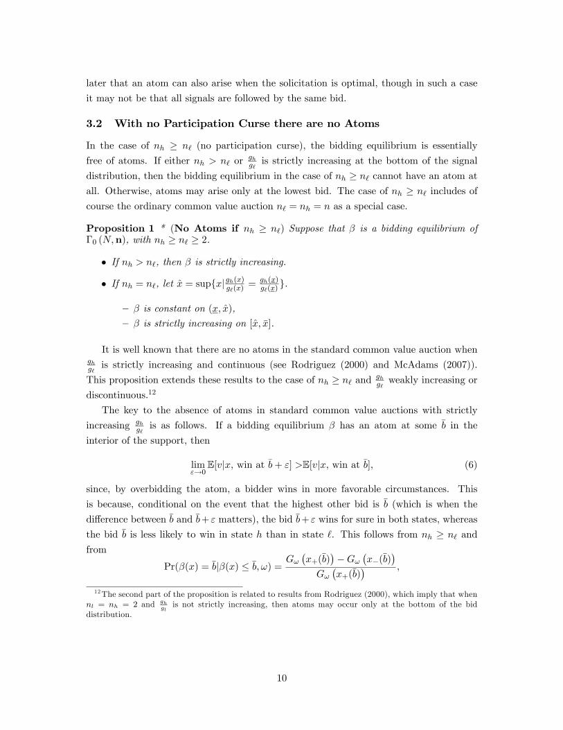
later that an atom can also arise when the solicitation is optimal, though in such a case

it may not be that all signals are followed by the same bid.

3.2 With no Participation Curse there are no Atoms

In the case of nh ≥ n` (no participation curse), the bidding equilibrium is essentially

free of atoms. If either nh > n` orghg`is strictly increasing at the bottom of the signal

distribution, then the bidding equilibrium in the case of nh ≥ n` cannot have an atom at

all. Otherwise, atoms may arise only at the lowest bid. The case of nh ≥ n` includes of

course the ordinary common value auction n` = nh = n as a special case.

Proposition 1 * (No Atoms if nh ≥ n`) Suppose that β is a bidding equilibrium ofΓ0 (N,n), with nh ≥ n` ≥ 2.

• If nh > n`, then β is strictly increasing.

• If nh = n`, let x̂ = sup{x|gh(x)g`(x) = gh(x)

g`(x) }.

— β is constant on (x, x̂),

— β is strictly increasing on [x̂, x̄].

It is well known that there are no atoms in the standard common value auction whenghg`is strictly increasing and continuous (see Rodriguez (2000) and McAdams (2007)).

This proposition extends these results to the case of nh ≥ n` and ghg`weakly increasing or

discontinuous.12

The key to the absence of atoms in standard common value auctions with strictly

increasing ghg`is as follows. If a bidding equilibrium β has an atom at some b̄ in the

interior of the support, then

limε→0

E[v|x, win at b̄+ ε] >E[v|x, win at b̄], (6)

since, by overbidding the atom, a bidder wins in more favorable circumstances. This

is because, conditional on the event that the highest other bid is b̄ (which is when the

difference between b̄ and b̄+ ε matters), the bid b̄+ ε wins for sure in both states, whereas

the bid b̄ is less likely to win in state h than in state `. This follows from nh ≥ n` and

from

Pr(β(x) = b̄|β(x) ≤ b̄, ω) =Gω(x+(b̄)

)−Gω

(x−(b̄)

)Gω(x+(b̄)

) ,

12The second part of the proposition is related to results from Rodriguez (2000), which imply that whennl = nh = 2 and gh

glis not strictly increasing, then atoms may occur only at the bottom of the bid

distribution.

10

being higher for ω = h than for ω = ` when ghg`is strictly increasing.13 Therefore,

overbidding b̄ is profitable, since it strictly increases both the expected value conditional

on winning (by (6)) and the probability of winning.

Thus, in the case of nh > n` orgh(x)g`(x) > gh(x)

g`(x) , the incentive to overbid an atom is

generated both by the improved selection of types at the higher bid, as captured by (6),

and by the usual Bertrand logic of a discrete jump in the winning probability. Conversely,

as illustrated by the example in the beginning of this section, when nh < n`, an atom

may be stable because (6) is reversed, and the worse selection of types following a slight

overbid overwhelms the Bertrand effect.

4 The Full Game, Optimal Solicitation and Large Numbers

This section introduces formally the full game and its equilibrium as well as some basic

steps towards the subsequent derivation of the characterization results.

4.1 The Full Game and Equilibrium

Let Γ (s) be the full game that includes both strategic bidder solicitation by the seller and

strategic bidding by the buyers. A bidding strategy β is as before; a solicitation strategy

n = (n`, nh) prescribes the number of bidders solicited by the seller in each state. The

potential number of bidders in Γ (s) is Ns with Ns ≥ vhs , which guarantees that it is never

profitable for the seller to solicit all potential bidders. Also, let E [p|ω;β, n] denote the

expected winning bid in state ω.

A pure equilibrium of Γ (s) consists of a non-decreasing bidding strategy β and a

solicitation strategy n = (n`, nh) such that (i) β is a bidding equilibrium of Γ0 (Ns,n),

and (ii) the solicitation strategy is optimal for the seller,

nω ∈ arg maxn∈{1,2,...,Ns}

E [p|ω;β, n]− ns.

Since a pure equilibrium might not exist, we allow for mixed solicitation strategies.

Let η = (η`, ηh) denote a mixed solicitation strategy, where ηω(n) is the probability with

which n = 1, ..., Ns bidders are invited in state ω.

The expected payoff U(b|x;β,η) and the probability of winning πω (b|β,η) are now

functions of the mixed strategy η. Some explicit expressions of these magnitudes that are

needed for the proofs are stated in Subsection 8.2 of the appendix.

13 In the special case where nh = n` andgh(x)g`(x)

= gh(x)g`(x)

for all signals x for which β (x) ≤ b̄, (6) holds as

an equality. In this case,Gω(x+)−Gω(x−)

Gω(x+), is the same in both states.

11

In a complete analogy to the definitions for pure strategies, Γ0 (N,η) is the bidding

game given η = (η`, ηh) and Γ (s) is the full game. A bidding equilibrium of Γ0 (N,η) is

a strategy β such that, for all x, b = β (x) maximizes U(b|x;β,η).

The strategy profile (β,η) is an equilibrium of Γ (s) if (i) β is a bidding equilibrium of

Γ0 (Ns,η) and (ii) the solicitation strategy is optimal,

ηω (n) > 0⇒ n ∈ arg maxn∈{1,2,...,Ns}

E [p|ω;β, n]− ns.

4.2 Optimal Solicitation: Characterization

The seller’s payoff, E [p|ω;β, n] − ns, is strictly concave in n unless β is constant. Con-sequently, either there is a unique optimal number of sampled bidders or the optimum is

attained at two adjacent integers.

Lemma 1 * Optimal Solicitation Given any bidding strategy β, there is an integer n∗ωsuch that

{n∗ω, n∗ω + 1} ⊇ arg maxn∈{1,2,··· ,N}

E [p|ω;β, n]− ns.

This result is familiar from other contexts and is an immediate consequence of the

concavity of the expectation of the first-order statistic in n, but a self contained proof is

provided in the online appendix. Given the lemma, we restrict attention to mixed strate-

gies η whose support contains at most two adjacent integers. Any such mixed strategy

ηω can be described by nω ∈ {1, ..., N} and γω ∈ (0, 1], where γω = ηω (nω) > 0 and

1 − γω = ηω (nω + 1) ≥ 0. A solicitation strategy is pure if γω = 1. Thus, from here on,

when we talk about nω in the context of a strategy ηω, we mean the bottom of the support

of ηω. In fact, since our characterization results pertain to the case of small sampling costs

and many bidders, they are not affected by whether the equilibrium strategies are actually

pure or mixed. Mixed solicitation strategies matter only for the existence arguments.14

4.3 Many Bidders

From here on the discussion focuses on scenarios with many bidders. From a substantive

point of view, this is the relevant case for the questions of competitiveness and information

aggregation in markets. From an analytical point of view, this case makes it easier to get

clean characterization results.

In Section 5 we consider the full game where the number of bidders is determined

endogenously. The primitive there is a sequence(sk)∞k=1

, sk > 0 and sk → 0, (7)

14The irrelevance of mixing for the case of many bidders is a formal result, which is not included in thispaper.

12

that induces a sequence of games Γ(sk)and a corresponding sequence of equilibrium

bidding and solicitation strategies (βk,ηk) with ηk = (ηk` , ηkh). It turns out that, as

sk → 0, the optimal solicitation would indeed result in ever larger numbers of solicited

bidders.

In Section 6 the state dependent numbers of bidders are exogenous. We look at a

sequence of bidding games

Γ0

(Nk,nk

)s.t. nkω →∞, ω = `, h,

and a corresponding sequence of bidding equilibria βk.

In either of those cases, we look at the limits of equilibrium magnitudes as k →∞. Forthe sake of reducing the complexity, we make the following simplifications. First, when we

discuss a fixed sequence (βk,ηk), and there is no danger of confusion, magnitudes induced

by (βk,ηk) is written as Uk(b|x), πkω(b), Ek[v|x,win at b] etc. (rather than U(b|x;βk,ηk)

etc.). Second, the term “limit” (and the operator lim) always refers to a limit over any

subsequence such that all the magnitudes of interest are converging, though we will not

repeat this qualification each time. Third, since almost all limits we take are with respect

to k, we often omit the delimiter k →∞ from the expression lim.

5 Atoms in Full Equilibrium: Failure of Information Aggre-gation

This section shows that, under certain conditions, an atom may arise in full equilibrium.

This means that strategic solicitation does not prevent the failure of the price to aggregate

information.

The example in Section 3.1 established the possibility of atoms in a bidding equilib-rium, but it was not a full equilibrium. The seller’s best response to that bidding behavior

is to solicit only one bid, which of course would not in turn induce that bidding behavior.

Some reflection would reveal that it is not straightforward to extend a bidding equilibrium

into a full equilibrium since it is not easy to see why the pattern of solicitation required

to sustain an atom in the bidding equilibrium would indeed be optimal given the bid-

ding it induces. Our approach is constructive. Under certain assumptions– including a

suffi ciently small solicitation cost– we construct a full equilibrium that exhibits an atom.

The main ideas can be presented in the context of a simple case with two effective

signals. We will therefore do so, although the same results are also valid for a more

general model.

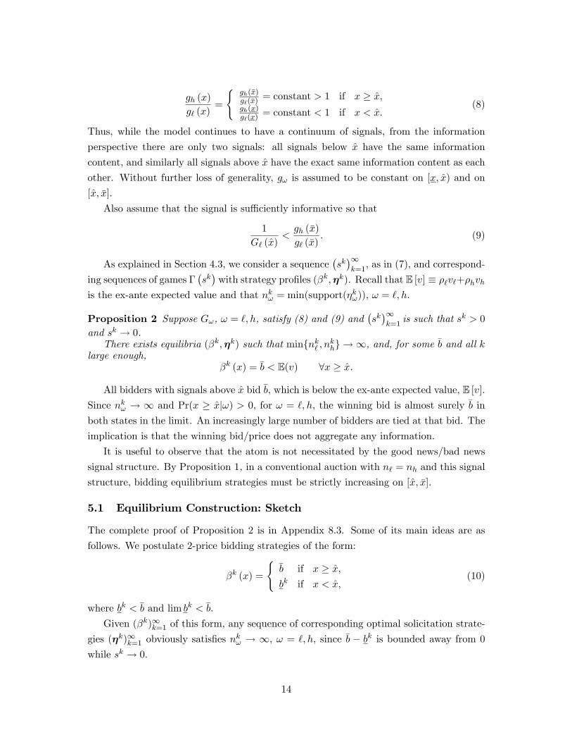
Good News/Bad News Signal. In the “good news/bad news”case considered here,there is some x̂ ∈ (x, x̄) such that

13

gh (x)

g` (x)=

{gh(x̄)g`(x̄) = constant > 1 if x ≥ x̂,gh(x)g`(x) = constant < 1 if x < x̂.

(8)

Thus, while the model continues to have a continuum of signals, from the information

perspective there are only two signals: all signals below x̂ have the same information

content, and similarly all signals above x̂ have the exact same information content as each

other. Without further loss of generality, gω is assumed to be constant on [x, x̂) and on

[x̂, x̄].

Also assume that the signal is suffi ciently informative so that

1

G` (x̂)<gh (x̄)

g` (x̄). (9)

As explained in Section 4.3, we consider a sequence(sk)∞k=1, as in (7), and correspond-

ing sequences of games Γ(sk)with strategy profiles (βk,ηk). Recall that E [v] ≡ ρ`v`+ρhvh

is the ex-ante expected value and that nkω = min(support(ηkω)), ω = `, h.

Proposition 2 Suppose Gω, ω = `, h, satisfy (8) and (9) and(sk)∞k=1

is such that sk > 0

and sk → 0.There exists equilibria (βk,ηk) such that min{nk` , nkh} → ∞, and, for some b̄ and all k

large enough,βk (x) = b̄ < E(v) ∀x ≥ x̂.

All bidders with signals above x̂ bid b̄, which is below the ex-ante expected value, E [v].

Since nkω → ∞ and Pr(x ≥ x̂|ω) > 0, for ω = `, h, the winning bid is almost surely b̄ in

both states in the limit. An increasingly large number of bidders are tied at that bid. The

implication is that the winning bid/price does not aggregate any information.

It is useful to observe that the atom is not necessitated by the good news/bad news

signal structure. By Proposition 1, in a conventional auction with n` = nh and this signal

structure, bidding equilibrium strategies must be strictly increasing on [x̂, x̄].

5.1 Equilibrium Construction: Sketch

The complete proof of Proposition 2 is in Appendix 8.3. Some of its main ideas are as

follows. We postulate 2-price bidding strategies of the form:

βk (x) =

{b̄ if x ≥ x̂,bk if x < x̂,

(10)

where bk < b̄ and lim bk < b̄.

Given (βk)∞k=1 of this form, any sequence of corresponding optimal solicitation strate-

gies (ηk)∞k=1 obviously satisfies nkω → ∞, ω = `, h, since b̄ − bk is bounded away from 0

while sk → 0.

14

The key step of the proof is that for any (ηk)∞k=1 that is optimal given bidding strategies

of the form (10),gh (x̄)

g` (x̄)lim

nkhnk`

< 1, (11)

and limnkhnk`is independent of the choice of b̄ and (bk).

These observations are proven (in Step 3 of the proof of Proposition 2) using the

marginal conditions for solicitation optimality. Ignoring integer issues– which the formal

proof takes into account– the optimality conditions are

(G` (x̂))nk` (1−G` (x̂)) (b̄− bk) = sk,

(Gh (x̂))nkh (1−Gh (x̂)) (b̄− bk) = sk.

Substituting out sk from the two conditions and making a logarithmic transformation,

we get

nk` lnG` (x̂) + ln (1−G` (x̂)) = nkh lnGh (x̂) + ln (1−Gh (x̂)) .

Noticing that the first term on each side of the equation dominates the second since

nkω →∞, we get

limnkhnk`

=lnG` (x̂)

lnGh (x̂). (12)

Thus, limnkhnk`

< 1, and the limit is independent of the choice of choice of b̄ and(bk).

Inequality (11) then follows from (12), via gh(x̄)g`(x̄) = 1−Gh(x̂)

1−G`(x̂) and1−zln z being a decreasing

function of z over (0, 1).

The significance of inequality (11) is that, for large enough k, the bad news learned

from being solicited overwhelms the good news contained in the highest signal. Thus, a

bidder with the highest signal is more pessimistic than the prior, ρhρ`gh(x̄)g`(x̄)

nkhnk`

< ρhρ`. As we

will see, this “overwhelming participation curse”creates an impediment to overbidding.

Another step in proving Proposition 2 is the choice of b̄ that would make overbidding it

unprofitable. For any (βk)∞k=1 of the form (10) and any corresponding optimal solicitation

strategies(ηk)∞k=1,

limEk[v|x̄,win at b̄] = E [v] > limEk[ v | x̄, win at b′ > b̄]. (13)

The inequality owes to (11): the likelihood ratio of a bidder with x̄ who wins at b′,ρhρ`

gh(x̄)g`(x̄)

nkhnk`, is lower than the prior likelihood ratio, ρhρ` , and this translates to an expected

value that is below the ex-ante expected value. The equality in (13) owes to the winning

probabilities at b̄ being roughly inversely proportional to the number of bidders bidding

15

b̄, i.e., for large k,

πkh(b̄)

πk` (b̄)≈

1nkh(1−Gh(x̂))

1nk` (1−G`(x̂))

=nk`nkh

g` (x̄)

gh (x̄).

It follows that the likelihood ratio of a bidder with x̄ who wins b̄ is approximately equal

to the prior one,ρhρ`

nkhnk`

gh (x̄)

g` (x̄)

πkh(b̄)

πk` (b̄)≈ρhρ`.

That is, the information learned from winning at b̄ exactly offsets the information learned

from being solicited and having a signal x ≥ x̂, and this translates to an expected value

that is approximately equal to the ex-ante expected value, E [v].15

The significance of these two observations is that b̄ can be chosen to satisfy

E [v] > b̄ > limEk[ v | x̄, win at b′],

making it profitable for bidders with x ≥ x̂ to bid b̄ and unprofitable to overbid it.The foregoing explanation presents the more special element in the proof of Proposition

2, capturing the role of the strategic solicitation in generating an atom. To complete the

proof, it is verified (in the appendix) that, given any such b̄, one can choose a sequence(bk)with lim bk < b̄ such that the resulting

(βk)together with the corresponding optimal

solicitations(ηk)are immune against all other deviations for all values of x.

5.2 Pooling with Many Signals

The assumption that the likelihood ratio takes only two values is not required to establish

the existence of a pooling equilibrium. A similar result can be derived in an environment

in which the likelihood ratio is a step function with an arbitrary of number steps. One

can also allow for an unbounded likelihood ratio, with gh(x̄)g`(x̄) = ∞. The construction of

the atom at the top and the argument for why optimal solicitation results in a ratio nkhnk`

that deters even recipients of the best signal from overbidding that atom are essentially

as outlined above for the two-signal case. The analysis of the multi-signal case is more

complicated in the parts dealing with equilibrium behavior below the atom; see Lauermann

and Wolinsky (2013).

6 General Characterization of Bidding Equilibria

We return now to discuss bidding equilibria. As mentioned in the introduction, state

dependent participation may arise for a number of reasons. Therefore, the understanding

15Alternatively, the equality in (13) follows from the law of iterated expectations. In the limit, as k →∞,almost surely the winner has a signal x > x̂ in both states. Thus, this event contains no information aboutthe state, and the posterior probability conditional on it is equal to the prior.

16

of bidding equilibria under such circumstances is of interest in its own right, independently

of a specific underlying process that determines the participation. We consider a sequence

of bidding games Γ0

(Nk,nk

)such that nkω → ∞, ω = `, h, and lim

nkhnk`∈ (0,∞) exists.16

With “many” bidders, only bids associated with signals that are suffi ciently close to x̄

would have significant probability of winning. Therefore, the object of interest is the

equilibrium distribution of the winning bid

Fω (p|β, n) =(Gω

(xk+(p)

))n,

and its limits, rather than the distribution of all the bids. We use the shorthand F kω (p)

for Fω(p|βk, nkω

), as we are doing for other functions.

6.1 Winning Bid Distribution: Pooling vs. Separating

Our main results expose a sharp relationship between nkhnk`and the form of F kω (p). For large

k, this distribution exhibits a large atom at the top if

limnkhnk`

gh (x̄)

g` (x̄)< 1, (14)

and is free of atoms if the reverse inequality holds.

The following proposition states this characterization result. Recall that xk−(b) =

inf{x|βk(x) ≥ b} and xk+(b) = sup{x|βk(x) ≤ b}. Thus, if F kω has an atom at b,

Pr(winning bid in k-th auction = b|ω) = Gω(xk+(b))nkω −Gω(xk−(b))n

kω > 0.

Proposition 3 * Consider a sequence of bidding games Γ0

(Nk,nk

)such that min{nk` , nkh} →

∞ and a corresponding sequence of bidding equilibria βk.

1. If limnkhnk`

gh(x̄)g`(x̄) < 1, then there are bids (bk)∞k=1 such that, for large enough k, F

kω has

an atom at bk and

lim Pr(winning bid in k-th auction = bk|ω) = 1 for ω = `, h.

2. If limnkhnk`

gh(x̄)g`(x̄) > 1, then for every sequence of bids (bk)∞k=1,

lim Pr(winning bid in k-th auction = bk|ω) = 0 for ω = `, h.

The proof is relegated to the online appendix. Part 1 does not mean that most bidders

are submitting the same bid, but rather that the probability of the atom’s bid is large

enough that it wins almost always.

16Since we are dealing only with bidding equilibria, we will restrict attention to pure solicitation ratherthan mixed. But all the results will be also valid for mixed solicitation strategies η such that the supportof ηw has at most two adjacent numbers, as must be the case for η’s that arise in a full equilibrium.

17

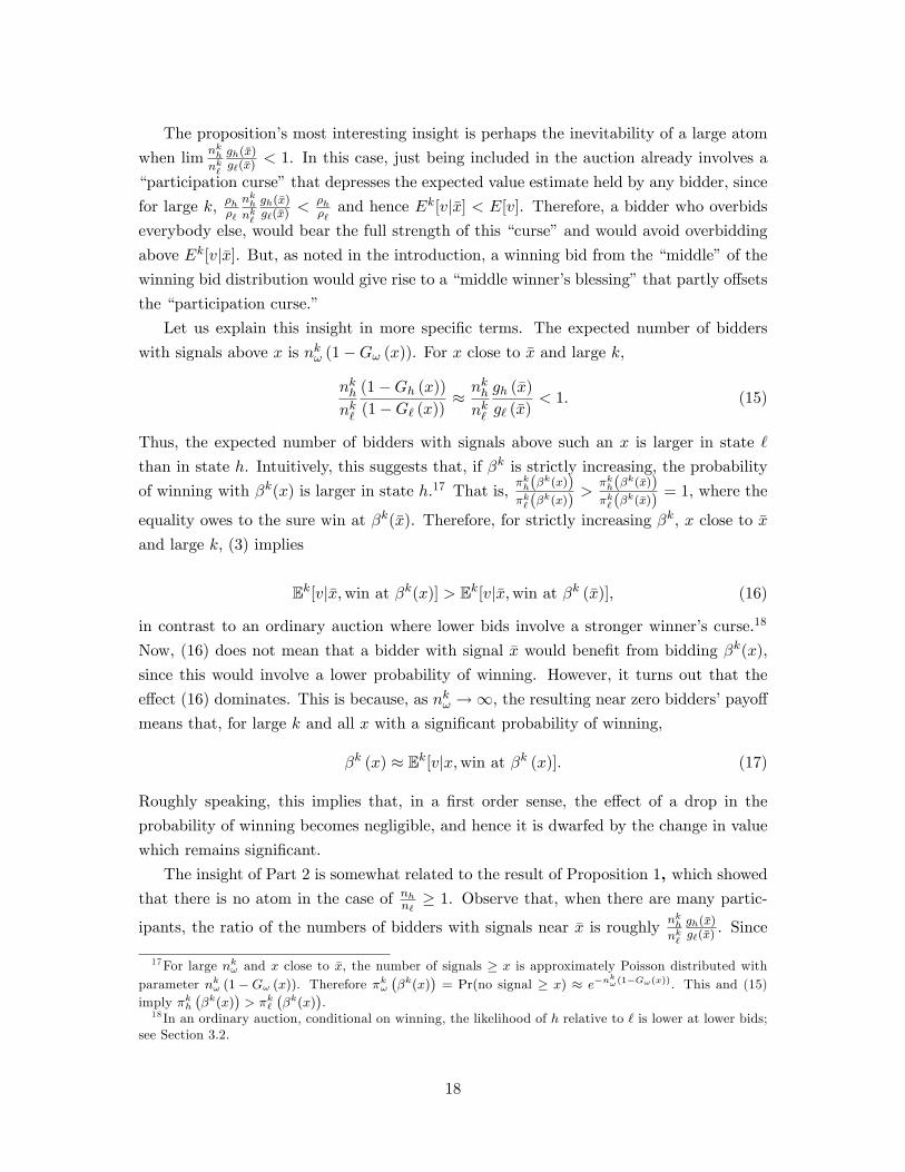
The proposition’s most interesting insight is perhaps the inevitability of a large atom

when limnkhnk`

gh(x̄)g`(x̄) < 1. In this case, just being included in the auction already involves a

“participation curse”that depresses the expected value estimate held by any bidder, since

for large k, ρhρ`nkhnk`

gh(x̄)g`(x̄) <

ρhρ`and hence Ek[v|x̄] < E[v]. Therefore, a bidder who overbids

everybody else, would bear the full strength of this “curse”and would avoid overbidding

above Ek[v|x̄]. But, as noted in the introduction, a winning bid from the “middle”of the

winning bid distribution would give rise to a “middle winner’s blessing”that partly offsets

the “participation curse.”

Let us explain this insight in more specific terms. The expected number of bidders

with signals above x is nkω (1−Gω (x)). For x close to x̄ and large k,

nkhnk`

(1−Gh (x))

(1−G` (x))≈ nkhnk`

gh (x̄)

g` (x̄)< 1. (15)

Thus, the expected number of bidders with signals above such an x is larger in state `

than in state h. Intuitively, this suggests that, if βk is strictly increasing, the probability

of winning with βk(x) is larger in state h.17 That is,πkh(β

k(x))πk` (β

k(x))>

πkh(βk(x̄))

πk` (βk(x̄))

= 1, where the

equality owes to the sure win at βk(x̄). Therefore, for strictly increasing βk, x close to x̄

and large k, (3) implies

Ek[v|x̄,win at βk(x)] > Ek[v|x̄,win at βk (x̄)], (16)

in contrast to an ordinary auction where lower bids involve a stronger winner’s curse.18

Now, (16) does not mean that a bidder with signal x̄ would benefit from bidding βk(x),

since this would involve a lower probability of winning. However, it turns out that the

effect (16) dominates. This is because, as nkω →∞, the resulting near zero bidders’payoffmeans that, for large k and all x with a significant probability of winning,

βk (x) ≈ Ek[v|x,win at βk (x)]. (17)

Roughly speaking, this implies that, in a first order sense, the effect of a drop in the

probability of winning becomes negligible, and hence it is dwarfed by the change in value

which remains significant.

The insight of Part 2 is somewhat related to the result of Proposition 1, which showedthat there is no atom in the case of nhn` ≥ 1. Observe that, when there are many partic-

ipants, the ratio of the numbers of bidders with signals near x̄ is roughly nkhnk`

gh(x̄)g`(x̄) . Since

17For large nkω and x close to x̄, the number of signals ≥ x is approximately Poisson distributed withparameter nkω (1−Gω (x)). Therefore πkω

(βk(x)

)= Pr(no signal ≥ x) ≈ e−n

kω(1−Gω(x)). This and (15)

imply πkh(βk(x)

)> πk`

(βk(x)

).

18 In an ordinary auction, conditional on winning, the likelihood of h relative to ` is lower at lower bids;see Section 3.2.

18

these bidders are the effective participants, lim nkhnk`

gh(x̄)g`(x̄) > 1 is in some sense the counterpart

of the condition from Proposition 1, and a similar intuition applies.

6.2 Expected Revenue and Prices in Large Auctions

Proposition 3 has straightforward implications for the equilibrium prices and revenues.

In the “pooling” case“ of limnkhnk`

gh(x̄)g`(x̄) < 1, the auction ends almost certainly with the

winning bid bk in both states. Bidders’individual rationality then implies lim bk ≤ E [v],

for otherwise bidders’ expected ex-ante payoff would be negative. And, as has already

been observed (Sections 3.1 and 5.1), this inequality may be strict.

In the “separating”case of limnkhnk`

gh(x̄)g`(x̄) > 1, the auction ends almost certainly with no

tie at the winning bid and, from (17), βk(x) ≈ Ek[v|x,win at βk(x)], for large k and for x

with a significant winning probability.

These observations have immediate implications for the seller’s expected revenue Ek[p|ω] ≡E[p|ω;βk, nkω

]for large k. In the “pooling”case, the revenue is the same across the states

and may be strictly below the ex-ante expected value, E [v]. In the “separating” case,

the seller’s ex-ante revenue is approximately equal to the ex-ante expected value, and the

interim expected revenue is higher in state h.

Proposition 4 Consider a sequence of bidding games Γ0

(Nk,nk

)such that min{nk` , nkh} →

∞ and a corresponding sequence of bidding equilibria βk.

1. If limnkhnk`

gh(x̄)g`(x̄) < 1, then

limEk[p|`] = limEk[p|h] ≤ E [v] .

2. If limnkhnk`

gh(x̄)g`(x̄) > 1, then

limEk[p|`] < E [v] < limEk[p|h],

andρ` limEk[p|`] + ρh limEk[p|h] = E [v] .

The proof of the proposition is instructive about the intuition and is therefore presented

here without further explanation.

Proof: Part 1 is an immediate corollary of Part 1 of Proposition 3. It follows from the

individual rationality of optimal bids.

For the cases covered by Part 2, we have already noted in (17) that, for high k and for

x with a significant probability of winning, βk(x) ≈ Ek[v|x,win at βk(x)]. Let y[nk] be the

19

random variable describing the highest signal given participation nk = (nk` , nkh).19 Then

βk (x) ≈ E[v|y[nk] = x;βk,nk] ≡ Ek[v|y[nk] = x]. (18)

Observe that, for large k,20

Ek[p|ω] = E[βk(y[nk])|ω

]≈ E

[Ek[v|y[nk]]|ω

]. (19)

This implies the equality of the ex-ante expected revenue to the ex-ante expected value:

E(Ek[p|ω]

)= E

(E[Ek[v|y[nk]]|ω

])= E [v], which is just an instant of the law of iterated

expectations

To establish limEk[p|h] > limEk[p|`], it is useful to argue in terms of the quantilesof the distribution, since the set of relevant x’s (with significant winning probability)

converges to x̄. So, let xk (α) denote the α-quantile of the distribution of y[nk]|`. That is,

for any α ∈ (0, 1), xk (α) is defined by(G`(xk (α)

))nk` = α.

Rewriting the expected value on the right-hand side of (19) as an integral and changing

the integration variable via the transformation α =(G`(xk (α)

))nk` ,Ek[p|`] ≈

∫ x̄

xEk[v|y[nk] = x]d(G`(x))n` =

∫ 1

0Ek[v|y[nk] = xk (α)]dα,

Ek[p|h] ≈∫ x̄

xEk[v|y[nk] = x]d(Gh(x))nh =

∫ 1

0Ek[v|y[nk] = xk (α)]d

(Gh

(xk (α)

))nkh.

The final step in the proof derives the limits of(Gh(xk (α)

))nkh and Ek[v|y[nk] = xk (α)].

Obviously, xk (α)→ x̄. Therefore,

lim

(1−Gh

(xk (α)

))nkh

(1−G` (xk (α)))nk`= lim

nkhnk`

gh (x̄)

g` (x̄)≡ λ > 1. (20)

Since for large k,21 (Gω

(xk (α)

))nkω ≈ e− lim(1−Gω(xk(α)))nkω ,

(20) implies (Gh

(xk (α)

))nkh ≈ [(G` (xk (α)))nk` ]λ

= αλ.

19y[nk] is not an ordinary first order statistic: In state ω, it is the first order statistic x(nkω).20Note that here Ek[v|y[nk]] is a random variable while Ek[v|y[nk] = x] is a number.21Recall that limn→∞

(1− (1−xn)n

n

)n= e− limn(1−xn) given any sequence (xn) with limn→∞ xn = 1.

20

From (3), we have

Ek[v|y[nk] = x] =

v` + ρhρ`

gh(x)g`(x)

nkhnk`

(Gh(x))nkh−1

(G`(x))nk`−1vh

1 + ρhρ`

gh(x)g`(x)

nkhnk`

(Gh(x))nkh−1

(G`(x))nk`−1

.

Since xk (α)→ x̄ and hence(G`(xk (α)

))nk` ≈ (G` (xk (α)))nk`−1

for large k,

limEk[v|y[nk] = xk (α)] =v` + ρh

ρ`λα

λ

α vh

1 + ρhρ`λα

λ

α

.

Therefore,

limEk[p|`] =

∫ 1

0limEk[v|y[nk] = xk (α)]dα, (21)

limEk[p|h] =

∫ 1

0limEk[v|y[nk] = xk (α)]d(αλ). (22)

Now, limEk[p|h] > limEk[p|`] follows because limEk[v|y[nk] = xk (α)] is a strictly

increasing function of α and the measure d(αλ)stochastically dominates the measure dα.

6.3 The Extent of Information Aggregation

As a fairly immediate corollary of the above arguments, we get the following observation

on the extent of information aggregation by the price.

Proposition 5 Consider a sequence of bidding games Γ0

(Nk,nk

)such that min{nk` , nkh} →

∞ and limnkhnk`

gh(x̄)g`(x̄) > 1, and a corresponding sequence of bidding equilibria βk. For any

ε > 0, there are ∆ and δ such that ∆ > δ > 1 and

if limnkhnk`

gh (x̄)

g` (x̄)> ∆, then | limEk[p|ω]− vω |< ε, ω = `, h,

if limnkhnk`

gh (x̄)

g` (x̄)< δ, then | limEk[p|ω]− E [v] |< ε, ω = `, h.

Thus, in the separating case of limnkhnk`

gh(x̄)g`(x̄) > 1, the price aggregates the information

well when limnkhnk`

gh(x̄)g`(x̄) is large and poorly when it is near 1. Of course, we already know

from Proposition 3 that, in the case of limnkhnk`

gh(x̄)g`(x̄) < 1 that is not covered by Proposition

5, the price fails to aggregate the information.

Proof: The first part of the proposition follows from limEk[v|y[nk] = xk (α)] ∼= E [v] for

all α when λ is close to one and from equations (21) and (22). The second part follows

21

from limEk[v|y[nk] = xk (α)] ∼= v` for all α < 1 for large λ. This and (21) implies that

limEk[p|`] ∼= v` for large λ. Then, the equality of the ex-ante expected revenue and E [v]

from the second part of Proposition 4 requires limEk[p|h] ∼= vh.

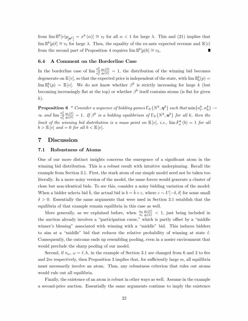
6.4 A Comment on the Borderline Case

In the borderline case of limnkhnk`

gh(x̄)g`(x̄) = 1, the distribution of the winning bid becomes

degenerate on E [v], so that the expected price is independent of the state, with limEkh(p) =

limEk` (p) = E [v]. We do not know whether βk is strictly increasing for large k (but

becoming increasingly flat at the top) or whether βk itself contains atoms (is flat for given

k).

Proposition 6 * Consider a sequence of bidding games Γ0

(Nk,ηk

)such that min{nk` , nkh} →

∞ and limnkhnk`

gh(x̄)g`(x̄) = 1. If βk is a bidding equilibrium of Γ0

(Nk,nk

)for all k, then the

limit of the winning bid distribution is a mass point on E [v], i.e., limF kω (b) = 1 for allb > E [v] and = 0 for all b < E [v].

7 Discussion

7.1 Robustness of Atoms

One of our more distinct insights concerns the emergence of a significant atom in the

winning bid distribution. This is a robust result with intuitive underpinning. Recall the

example from Section 3.1. First, the stark atom of our simple model need not be taken too

literally. In a more noisy version of the model, the same forces would generate a cluster of

close but non-identical bids. To see this, consider a noisy bidding variation of the model:

When a bidder selects bid b̂, the actual bid is b = b̂+ ε, where ε ∼ U [−δ, δ] for some smallδ > 0. Essentially the same arguments that were used in Section 3.1 establish that the

equilibria of that example remain equilibria in this case as well.

More generally, as we explained before, when nhn`

gh(x̄)g`(x̄) < 1, just being included in

the auction already involves a “participation curse,”which is partly offset by a “middle

winner’s blessing” associated with winning with a “middle” bid. This induces bidders

to aim at a “middle” bid that reduces the relative probability of winning at state `.

Consequently, the outcome ends up resembling pooling, even in a nosier environment that

would preclude the sharp pooling of our model.

Second, if nω, ω = `, h, in the example of Section 3.1 are changed from 6 and 2 to 6m

and 2m respectively, then Proposition 3 implies that, for suffi ciently large m, all equilibria

must necessarily involve an atom. Thus, any robustness criterion that rules out atoms

would rule out all equilibria.

Finally, the existence of an atom is robust in other ways as well. Assume in the example

a second-price auction. Essentially the same arguments continue to imply the existence

22

of equilibrium with an atom. In particular, a bidder who overbids the atom at b̄ wins in

both states, and pays b̄, which exceeds the expected value conditional on winning.

7.2 Affi liation of First-Order Statistic and State

The emergence of atoms can be also explained by the failure of the affi liation between the

value and the highest signal. Recall that y[n] denotes the highest signal realization given

participation n = (n`, nh). The likelihood ratio conditional on y[n] = x is

nhn`

gh (x)

g` (x)

(Gh (x))nh−1

(G` (x))n`−1 . (23)

In standard auctions with nh = n` = n, this likelihood ratio is increasing in x. Thus, the

statistic y[n], which in this case coincides with the first order statistic x(n), is affi liated

with the value. In contrast, with state dependent participation, the likelihood ratio (23)

need not be increasing– it is in fact decreasing for x suffi ciently close to x̄ if nhn`gh(x̄)g`(x̄) < 1.

Therefore, y[n] might not be affi liated with the value.

7.3 Signaling: Observable Number of Bidders

In a variation on our model in which the seller’s solicitation of n bidders is observed prior

to the bidding,22 there are two types of pure strategy signaling equilibria– separating and

pooling. In the pooling equilibrium, n` = nh. The pooling equilibria are the same as

those of the standard common value auction, since n is independent of the state. Multiple

pooling equilibria can be supported by off-path beliefs that place probability 1 on state `

following a seller’s deviation. In the separating equilibrium, n` = 2 and nh > 2, bidders

bid v` and vh respectively and the seller’s payoff is v` − 2s in both states. Therefore, if s

is small, the seller’s revenue is lower than it is when n is not observable, as in the model

of this paper. Incentive compatibility requires vh−nhs = v`− 2s, which, owing to integer

constraints, may hold only for special configurations of s, v` and vh.23

7.4 Sticky Prices

The phenomenon of “sticky prices”– prices that do not respond to changes in the funda-

mentals of the environment has been commonly explained in the relevant literatures by

the presence of menu costs. Our analysis suggests another source– adverse selection– for

explaining this phenomenon. This is seen through the fact that in the pooling equilibrium

22The focus of this paper is trading on environments in which the seller cannot verifiably communicatethe number of solicited bidders. The variation of this subsection is merely an exercise aimed at providingsharper understanding of the model.23But there always exists a nearby partially separating mixed strategy equilibrium in which the seller

mixes slightly between n` and nh, the bids are the expected value conditional on the observed number andthe seller’s payoff is close to v` − 2s.

23

identified in this paper trade may take place (almost certainly) at some b̄ < E [v], which

need not be sensitive to (small) changes in the fundamentals– the values vω and the prior

ρω.

7.5 Information Aggregation and Effi ciency

In the simple common values environment of this paper, it is effi cient to transfer the unit

to any buyer and this transfer indeed occurs in equilibrium regardless of how well the

information is aggregated. But this does not mean that the question of information aggre-

gation has no importance in a common values environment. Straightforward enrichments

of the simple model of this paper will introduce effi ciency consequences for information

aggregation. For example, if the seller’s cost is c ∈ (v`, vh), effi ciency requires that trade

takes place only in state h. In this case, a failure of information aggregation implies al-

locative ineffi ciencies. Alternatively, if the seller has an opportunity to invest in quality

improvements prior to trade, a failure of information aggregation could imply ineffi ciently

weak investment incentives.

8 Appendix

8.1 Winning Probability at Atoms

The following lemma derives an expression for the winning probability in the case of a tie.

Recall from (5) that x+(b) = sup{x|β(x) ≤ b} and x−(b) = inf{x|β(x) ≥ b}, so that anatom at b means x−(b) < x+(b). We omit the argument and write x− and x+ when it is

clear from the context.

Lemma 2 Suppose β is non-decreasing and, for some b̄, x−(b̄)< x+

(b̄). Then,

πω(b̄|β, n

)=

Gω (x+)n −Gω (x−)n

n (Gω (x+)−Gω (x−))=

∫ x+

x−

(Gω (x))n−1 gω (x) dx

Gω (x+)−Gω (x−). (24)

Observe that the last expression is the expected probability of a randomly drawn signal

from [x+, x−] to be the highest. Thus, πω(b̄|β, n

)“averages”what would be the winning

probabilities of the types in [x+, x−], if β were strictly increasing.

24

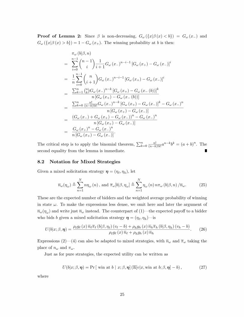
Proof of Lemma 2: Since β is non-decreasing, Gω ({x|β (x) < b}) = Gω (x−) and

Gω ({x|β (x) > b}) = 1−Gω (x+). The winning probability at b is then:

πω (b|β, n)

=

n−1∑i=0

(n− 1

i

)1

i+ 1Gω (x−)n−i−1 [Gω (x+)−Gω (x−)]i

=1

n

n−1∑i=0

(n

i+ 1

)Gω (x−)n−i−1 [Gω (x+)−Gω (x−)]i

=

∑nk=1

(nk

)Gω (x−)n−k [Gω (x+)−Gω (x− (b))]k

n [Gω (x+)−Gω (x− (b))]

=

∑nk=0

n!(n−k)!k!Gω (x−)n−k [Gω (x+)−Gω (x−)]k −Gω (x−)n

n [Gω (x+)−Gω (x−)]

=(Gω (x−) +Gω (x+)−Gω (x−))n −Gω (x−)n

n [Gω (x+)−Gω (x−)]

=Gω (x+)n −Gω (x−)n

n [Gω (x+)−Gω (x−)].

The critical step is to apply the binomial theorem,∑n

k=0n!

(n−k)!k!an−kbk = (a+ b)n. The

second equality from the lemma is immediate.

8.2 Notation for Mixed Strategies

Given a mixed solicitation strategy η = (η`, ηh), let

nω(ηω) ,N∑n=1

nηω (n) , and πω[b|β, ηω] ,N∑n=1

ηω (n)nπω (b|β, n) /nω. (25)

These are the expected number of bidders and the weighted average probability of winning

in state ω. To make the expressions less dense, we omit here and later the argument of

nω(ηω) and write just nω instead. The counterpart of (1)– the expected payoff to a bidder

who bids b given a mixed solicitation strategy η = (η`, ηh)– is

U(b|x;β,η) =ρ`g` (x)n`π` (b|β, η`) (v` − b) + ρhgh (x)nhπh (b|β, ηh) (vh − b)

ρ`g` (x)n` + ρhgh (x)nh. (26)

Expressions (2)– (4) can also be adapted to mixed strategies, with nω and πω taking the

place of nω and πω.

Just as for pure strategies, the expected utility can be written as

U(b|x;β,η) = Pr [ win at b | x;β,η] (E[v|x,win at b;β,η]− b) , (27)

where

25

E[ v | x, win at b;β,η] =ρ`g` (x)n`π` (b|β, η`) v` + ρhgh (x)nhπh (b|β, ηh) vhρ`g` (x)n`π` (b|β, η`) + ρhgh (x)nhπh (b|β, ηh)

(28)

=v` + ρh

ρ`

gh(x)g`(x)

nhn`

πh(b|β,ηh)π`(b|β,η`)

vh

1 + ρhρ`

gh(x)g`(x)

nhn`

πh(b|β,ηh)π`(b|β,η`)

,

and

Pr [ win at b | x;β,η] =ρ`g` (x)n`π` (b|β, η`) + ρhgh (x)nhπh (b|β, ηh)

ρ`g` (x)n` + ρhgh (x)nh(29)

=π` (b|β, η`) + ρh

ρ`

gh(x)g`(x)

nhn`πh (b|β, ηh)

1 + ρhρ`

gh(x)g`(x)

nhn`

.

8.3 Pooling Equilibrium in the Full Game

Proof of Proposition 2: First, the proof derives implications for optimal solicitation(ηk)∞k=1 in the face of a 2-price bidding strategy β

k (x) and sk → 0. Then, it identifies

values of bk and b̄ with which βk (x) is a bidding equilibrium, given a solicitation strategy

of the form derived above. Finally, a fixed-point argument is used to confirm existence.

Recall that lim sk = 0 by the hypothesis of the proposition. In what follows we consider(βk,ηk

)∞k=1

such that

βk (x) =

{b̄ if x ≥ x̂bk if x < x̂,

bk < b̄ and lim bk < b̄,

ηk is optimal given βk and sk.

(30)

Recall that the support of ηω is {nω, nω + 1} with γω = ηω (nω) > 0.

Step 1: For every k with nkω ≥ 2,

(1−G` (x̂))

(1−Gh (x̂))

1

Gh (x̂)≥ Gh (x̂)n

kh−1

G` (x̂)nk`−1≥ G` (x̂)

(1−G` (x̂))

(1−Gh (x̂)), (31)

and,

if γk` < 1, thenGh (x̂)n

kh

G` (x̂)nk`

≤ (1−G` (x̂))

(1−Gh (x̂)). (32)

Proof of Step 1: Since nkω maximizes the seller’s expected payoff24, Eω

[p|βk, nkω

]−nkωs,

it satisfies

Eω[p|βk, nkω

]− Eω

[p|βk, nkω − 1

]≥ sk ≥ Eω

[p|βk, nkω + 1

]− Eω

[p|βk, nkω

]. (33)

24 In this proof, we will not omit the arguments βk, nkω of the functions like πω and Eω, since sometimes,as in the next equation, nkω is not fixed for all expressions.

26

Since, by (30),

Eω[p|βk, nkω

]=(

1−Gω (x̂)nkω

)b̄+Gω (x̂)n

kω bk,

(33) can be rewritten as

Gω (x̂)nkω−1 (1−Gω (x̂))

(b̄− bk

)≥ sk ≥ Gω (x̂)n

kω (1−Gω (x̂))

(b̄− bk

)ω = `, h.

(34)

Therefore,

Gh (x̂)nkh−1 (1−Gh (x̂)) ≥ G` (x̂)n

k` (1−G` (x̂)) ,

G` (x̂)nk`−1 (1−G` (x̂)) ≥ Gh (x̂)n

kh (1−Gh (x̂)) ,

which implies (31).

Now, if γk` < 1, then sk = G` (x̂)nk` (1−G` (x̂))

(b̄− bk

). Therefore, the last inequality

can be replaced by G` (x̂)nk` (1−G` (x̂)) ≥ Gh (x̂)n

kh (1−Gh (x̂)), yielding (32). �

Step 2: nkω →∞ for ω ∈ {`, h} .Proof of Step 2: Since lim sk = 0 and lim

(b̄− bk

)> 0, it follows from the second

inequality in (34)– which does not require nkω ≥ 2– that limGω (x̂)nkω = 0, so limnkω =∞.

�Step 3:

gh (x̄)

g` (x̄)lim

nkhnk`

< 1.

Proof of Step 3: From (31),

limGh (x̂)n

kh

G` (x̂)nk`

= lim

Gh (x̂)

nkhnk`

G` (x̂)

nk`

∈ (0,∞) .

Since nk` →∞, this requires that

limGh (x̂)

nkhnk`

G` (x̂)=Gh (x̂)

limnkhnk`

G` (x̂)= 1.

Applying a logarithmic transformation to both sides, lnGh (x̂) limnkhnk`

= lnG` (x̂). Hence,

limnkhnk`

=lnG` (x̂)

lnGh (x̂).

Therefore,

gh (x̄)

g` (x̄)lim

nkhnk`

=gh (x̄)

g` (x̄)

lnG` (x̂)

lnGh (x̂)=

1−Gh (x̂)

1−G` (x̂)

lnG` (x̂)

lnGh (x̂)< 1.

27

where the second equality follows from gh(x̄)g`(x̄) = gh(x̄)

g`(x̄)1−x̂1−x̂ = 1−Gh(x̂)

1−G`(x̂) and the inequality

follows from the fact that∣∣1−z

ln z

∣∣ is strictly increasing in z ∈ (0, 1) and that G` (x̂) > Gh (x̂).

�Step 4: Recall nω(ηω) and πω(b|β, ηω), ω = `, h, from (25).

limnkhnk`

= limnkhnk`

=lnG` (x̂)

lnGh (x̂). (35)

For all b ≥ bk,

limπh(b|βk, ηkh)

π`(b|βk, ηk` )= lim

γkhπh(b|βk, nkh) + (1− γkh)πh(b|βk, nkh + 1)

γk`π`(b|βk, nk` ) + (1− γk` )π`(b|β

k, nk` + 1), (36)

and

limπh(b̄|βk, ηkh)

π`(b̄|βk, ηk` )= lim

πh(b̄|βk, nkh)

π`(b̄|βk, nk` )= lim

nk`nkh

g` (x̄)

gh (x̄). (37)

Proof of Step 4: Since ηkω(nkω)

= γkω = 1 − ηkω(nkω + 1

), we have nkω = γkωn

kω + (1 −

γkω)(nkω + 1

). Steps 2 and 3 now imply (35).

To establish (36), rewrite the definition of πω to get

πω(b|βk, ηkω)

γkωπω(b|βk, nkω) + (1− γkω)πω(b|βk, nkω + 1)

=

nkωnkω

(γkωπω(b|βk, nkω) + (1− γkω)πω(b|βk, nkω + 1)

)+ (1−γkω)

nkωπω(b|βk, nkω + 1)

γkωπω(b|βk, nkω) + (1− γkω)πω(b|βk, nkω + 1).

Since, by Step 2, nkω →∞, the RHS converges to 1, implying (36).

To establish the second equality in (37), note that (24) implies πω(b̄|βk, nkω) = 1−Gω(x̂)nkω

nkω [1−Gω(x̂)].

Since Gω (x̂) < 1 and, by Step 2, nkω →∞, it follows that Gω (x̂)nkω → 0. Also, since signals

satisfy (8), 1−Gh(x̂)1−G`(x̂) = gh(x̄)

g`(x̄)1−x̂1−x̂ . Therefore, we have

limπh(b̄|βk, nkh)

π`(b̄|βk, nk` )= lim

nk`nkh

g` (x̄)

gh (x̄). (38)

For the first equality of (37), note that

limπω(b̄|βk, nkω + 1)

πω(b̄|βk, nkω)= lim

1−Gω(x̂)nkω+1

(nkω+1)[1−Gω(x̂)]

1−Gω(x̂)nkω

nkω [1−Gω(x̂)]

= 1. (39)

Now, (39) and (36) yield the desired equality. �

Steps 5-7 derive bounds, v∗, v∗∗ and v∗∗∗, on the (limits of the) expected values con-

28

ditional on winning at b̄, b′ > b̄, and bk, respectively. Importantly, these bounds hold

uniformly for all sequences(βk,ηk

)∞k=1

that satisfy (30).

Step 5: There exists a number v∗∗∗ < E [v] such that

limE[v| x, win at b̄;βk,ηk] =

{E [v] if x ≥ x̂,v∗∗∗ if x < x̂.

Proof of Step 5: Using (37) and (35) to evaluate the limit of (28),

limE[ v |x, win at b̄;βk,ηk] =v` + ρh

ρ`

gh(x)g`(x)

g`(x̄)gh(x̄)vh

1 + ρhρ`

gh(x)g`(x)

g`(x̄)gh(x̄)

. (40)

If x ≥ x̂, then gh(x)g`(x) = gh(x̄)

g`(x̄) , and hence the RHS = ρ`v` + ρhvh ≡ E [v], as claimed.

For x < x̂, define v∗∗∗ to be the RHS of (40) at x = x. Therefore, v∗∗∗ is independent

of the choice of(βk,ηk

)∞k=1, as required. Since gh(x)

g`(x)g`(x̄)gh(x̄) =

(gh(x)g`(x)

)/(gh(x̄)g`(x̄)

)< 1, we have

v∗∗∗ < ρ`v` + ρhvh ≡ E [v]. �Step 6: There exists a number v∗∗ < E [v] such that, for any x ≥ x̂,

limE[ v | x, win at b > b̄;βk,ηk] = v∗∗.

Proof of Step 6: For x ≥ x̂, gh(x)g`(x) = gh(x̄)

g`(x̄) . For b > b̄, π`(b|βk, ηk` ) = πh(b|βk, ηkh) = 1.

Thus, π̄h(bk|βk,ηkh)

π̄`(bk|βk,ηk` )= 1. Use both of these observations, Step 4 and (28) to get, for any

x ≥ x̂,

limE[ v | x, win at b > b̄;βk,ηk] =v` + ρh

ρ`

gh(x̄)g`(x̄)

lnG`(x̂)lnGh(x̂)vh

1 + ρhρ`

gh(x̄)g`(x̄)

lnG`(x̂)lnGh(x̂)

, v∗∗,

By Step 3, v∗∗ < ρ`v` + ρhvh ≡ E [v], and, by its definition, v∗∗ is independent of(βk,ηk

)∞k=1, as required. �

Step 7: There exists a number v∗ such that, for any x < x̂,

E[v|x, win at bk;βk,ηk

]≤ v∗ < E [v] .

Proof of Step 7: By (24), πω(bk|βk, n) = Gω(x̂)n−0n(Gω(x̂)−0) = Gω(x̂)n−1

n . Substituting this into

the definition of πω gives

πh(bk|βk, ηkh)

π`(bk|βk, ηk` )

=nk`nkh

γkhGh (x̂)nkh−1 + (1− γkh)Gh (x̂)n

kh

γk`G` (x̂)nk`−1 + (1− γk` )G` (x̂)n

k`

.

Then substituting this into (28) and noting that from (8), for x < x̂, gh(x)g`(x) = gh(x)

g`(x) = Gh(x̂)G`(x̂) ,

29

we get

E[v|x, win at bk;βk,ηk

]=

ρ`v` + ρhγkhGh(x̂)n

kh+(1−γkh)Gh(x̂)n

kh+1

γk`G`(x̂)nk` +(1−γk` )G`(x̂)

nk`

+1vh

ρ` + ρhγkhGh(x̂)

nkh+(1−γkh)Gh(x̂)

nkh

+1

γk`G`(x̂)nk` +(1−γk` )G`(x̂)

nk`

+1

. (41)

It follows from Step 1 that

γkhGh (x̂)nkh + (1− γkh)Gh (x̂)n

kh+1

γk`G` (x̂)nk` + (1− γk` )G` (x̂)n

k`+1

≤ 1

G` (x̂)

1−G` (x̂)

1−Gh (x̂).

Specifically, if γk` = 1, the LHS is bounded from above by Gh(x̂)nkh

G`(x̂)nk`and the inequality

follows from the first inequality in (31); if γk` < 1, the LHS is bounded from above byGh(x̂)n

kh

G`(x̂)nk`

+1and the inequality follows from (32). Hence,

E[v|x, win at bk;βk,ηk

]≤ ρ`

ρh1

G`(x̂)1−G`(x̂)1−Gh(x̂) + ρ`

v` +ρh

1G`(x̂)

1−G`(x̂)1−Gh(x̂)

ρh1

G`(x̂)1−G`(x̂)1−Gh(x̂) + ρ`

vh , v∗.

From Assumption (9), 1G`(x̂)

1−G`(x̂)1−Gh(x̂) < 1. Therefore, v∗ < ρ`v` + ρhvh ≡ E [v]. By its

definition, v∗ is independent of the choice of(βk,ηk

)∞k=1. �

The remaining steps use the bounds from Steps 5-7 to construct the equilibrium βk’s.

Step 8: If

bk = E[v| x,win at b = bk;βk,ηk] ≤ max {v∗, v∗∗, v∗∗∗} < b̄ < E [v] , (42)

then bidding b̄ is a best response for x ≥ x̂ and large k.Proof of Step 8: Fix some x ≥ x̂. From (26), Step 5, Step 6, (42), and the positive

winning probability at both b̄ and b′ > b̄, it follows that, for large k, U(b̄|x;βk,ηk) ≈Pr [ win at b̄ | x;βk,ηk](E [v] − b̄) > 0 and U(b′|x;βk,ηk) ≈ (v∗∗ − b′) < 0. Thus, it is

profitable to bid b̄, but unprofitable to overbid it.

Consider b′′ < b̄. From (26), U(b′′|x;βk,ηk) < Pr [ win at b′′ | x;βk,ηk]vh. By (29), for

any b, Pr [ win at b | x;βk,ηk] is a weighted sum of the π̄ω(b|βk, ηkω), ω = `, h, with weights

that are independent of b. By (24), for large k, π̄ω(b̄|βk, ηkω) is on the order of 1nkω(1−Gω(x̂))

,

while π̄ω(b′′|βk, ηkω) is at most on the order of Gω (x̂)nkω−1. Hence, π̄ω(b′′|βk,ηkω)

π̄ω(b̄|βk,ηkω)→ 0,

ω = `, h, implying Pr [ win at b′′ | x;βk,ηk]

Pr [ win at b̄ | x;βk,ηk]→ 0. This and E [v] − b̄ > 0 from (42) imply

U(b′′|x,βk,ηk)

U(b̄|x,βk,ηk)→ 0. Thus, there is no incentive to undercut b̄ for large k. �

Step 9: Bidding bk is a best response for x < x̂ and large k.

Proof of Step 9: Fix some x′ < x̂. By the choice of bk in (42), U(bk|x′, βk,ηk) = 0 for

all k. Consider now possible deviations. Obviously, for b < bk, U(b|x′, βk,ηk) = 0. From

30

Step 5 and (42), U(b̄|x′, βk,ηk) < 0 for large k. For b > b̄, it follows from gh(x′)g`(x′)

< gh(x̄)g`(x̄) ,

Step 6, and (42) that U(b|x′, βk,ηk) < U(b|x̄, βk,ηk) < 0 for large k.

For b ∈(bk, b̄

), πω(b|βk, n) = Gω (x̂)n−1. This and (36) imply

limπh(b|βk, ηkh)

π`(b|βk, ηk` )= lim

γkhGh (x̂)nkh−1 + (1− γkh)Gh (x̂)n

kh

γk`G` (x̂)nk`−1 + (1− γk` )G` (x̂)n

k`

.

Then, substitute this and gω (x′) = gω (x) = Gω (x̂) /x̂ into (28) to get

limE[v|x′, win at b ∈

(bk, b̄

);βk,ηk

]=

ρ`v` + ρh limnkhnk`

γkhGh(x̂)nkh+(1−γkh)Gh(x̂)n

kh+1

γk`G`(x̂)nk` +(1−γk` )G`(x̂)

nk`

+1vh

ρ` + ρh limnkhnk`

γkhGh(x̂)nkh+(1−γkh)Gh(x̂)

nkh

+1

γk`G`(x̂)nk` +(1−γk` )G`(x̂)

nk`

+1

.

This, together with (41), (42), and limnkhnk`< 1 (from Step 3) imply that for large k,

E[v|x′, win at b ∈

(bk, b̄

);βk,ηk

]< E

[v|x′, win at bk;βk,ηk

]= bk.

Hence, for b ∈(bk, b̄

), U(b|x′, βk,ηk) < 0. Thus, for any x′ < x̂ and large k, there is no

profitable deviation from bk. �Step 10: There exists a sequence

(βk,ηk

)∞k=1

that satisfies (30) and (42).

Proof of Step 10: Let v̂ :≡ max [v∗, v∗∗, v∗∗∗]. Steps 5-7 imply that, if(βk,ηk

)∞k=1

satisfies (30), then

E[v|x,win at bk;βk,ηk] ≤ v̂ < E [v] , (43)

Choose any b̄ to satisfy (42).

Given any b ∈ [0, v̂], let βb be as in (30) with bk = b and b̄ as fixed before. Define the

correspondence Ψkω : [0, v̂]⇒ ∆ {1, ..., Nsk} by

Ψkω (b) , arg max

η∈∆{1,...,Nsk}

∑η (n)

(Eω [p|βb, n]− nsk

),

and Ψk , Ψk` ×Ψk

h. Define the function b̂ : (∆ {1, ..., Nsk})2 × [0, v̂]→ [0, v̂] by

b̂ (η, b) = E [v| x, win at b;βb,η] .

By the theorem of the maximum and the continuity of the expected winning bid in η

and b, Ψk is a non-empty and upper hemicontinuous correspondence. By Lemma 1, it is

convex valued. A bidder’s posterior conditional on being solicited is continuous in η (note

that ηω (0) = 0 by definition) and hence b̂ (η, b) is continuous in η as well. The function

b̂ (η, b) is constant in b, since the expectation defining it is the same for all b, and b̂ maps

into [0, v̂] by (43).

Thus, (Ψk, b̂) is a non-empty, convex valued, and upper hemicontinuous correspondence

31

from(∆{

1, ..., N̄})2 × [0, v̂] into itself. Therefore, by Kakutani’s theorem it has a fixed

point. Denote one such fixed point as (ηk, bk). The fixed-point satisfies the requirements in

the statement of the Lemma: ηk is a best-response to βk for all k, and bk, b̄ are constructed

to satisfy (42), which also implies the remaining conditions of (30), namely, bk < b̄ and

lim bk < b̄. �

By Step 10, there exists a sequence(βk,ηk

)∞k=1

that satisfies (30) and (42). For all k

suffi ciently large,(βk,ηk

)forms an equilibrium: By (30), ηk is a best-response to βk for

all k. By Steps 8 and 9, βk is a best response to ηk for all k large enough. This completes

the proof.

ReferencesAtakan, A. and M. Ekmekci (2014), “Auctions, Actions, and the Failure of Information

Aggregation.”American Economic Review, 2014-2048.

Atakan, A. and M. Ekmekci (2015), “Market Selection and Information Content of Prices,

Mimeo.

Broecker, T. (1990), “Credit-Worthiness Tests and Interbank Competition,”Economet-

rica, 429-452.

Burdett, K. and K. Judd (1983), “Equilibrium Price Dispersion,”Econometrica, 955-969.

Comanor, W. and M. Schankerman (1976), “Identical Bids and Cartel Behavior,”The

Bell Journal of Economics, 281—286.

Kremer, I. (2002), “Information Aggregation in Common Value Auctions,”Econometrica,

1675—1682.

Lauermann, S. and A.Wolinsky (2013), “A Common Value Auction with Bidder Solicitation–

The Complete Analysis,”Working Paper.

Lauermann, S. and A. Wolinsky (2016), “Search with Adverse Selection,”Econometrica,

243—315.

McAdams, D. (2007), “Monotonicity in Asymmetric First-Price Auctions with Affi liation,”

International Journal of Game Theory, 427-453.

Milgrom, P. (1979), “A Convergence Theorem for Competitive Bidding with Differential

Information,”Econometrica, 679-688.

Milgrom, P. (1981): “Rational Expectations, Information Acquisition, and Competitive

Bidding,”Econometrica, 921-943.

Mund, V. (1960), “Identical Bid Prices,”Journal of Political Economy, 150—69.

Murto, P. and J. Välimäki (2015), “Common Value Auctions with Costly Entry,”Mimeo.

32

Riordan, M. (1993), “Competition and Bank Performance: A Theoretical Perspective,”in:

Capital Markets and Financial Intermediation, C. Mayer and X. Vives, eds., Cambridge

University Press, 328-343.

Rodriguez, G. (2000), “First Price Auctions: Monotonicity and Uniqueness,”International

Journal of Game Theory, 413-432.

Subramanian, G. (2010), “Negotiauctions: New dealmaking strategies for a competitive

marketplace,”WW Norton & Company.

Wilson, R. (1977), “A Bidding Model of Perfect Competition,”Review of Economic Stud-

ies, 511-518.

33

9 Appendix– For Online Publication Only

9.1 Proof of Proposition 1

Proof of Proposition 1: Suppose that nh ≥ n` ≥ 2 and β is a non-decreasing bidding

equilibrium given (n`, nh).

Recall from (5) that x+(b) = sup{x|β(x) = b} and x−(b) = inf{x|β(x) = b}, so thatan atom at b means x−(b) < x+(b). We omit the arguments and write x− and x+ when

it is clear from the context.

Step 1: Gh(x)nh

G`(x)n`is weakly increasing on any interval (y, z) if n` ≤ nh. It is constant if

and only if n` = nh andgh(x)g`(x) = gh(x)

g`(x) for all x < z.

Proof of Step 1: For z > y,

Gh(z)nh

G` (z)n`− Gh(y)nh

G` (y)n`=

(Gh(z)

G` (z)

)n`(Gh(z))nh−n` −

(Gh(y)

G` (y)

)n`(Gh(y))nh−n`

≥(Gh(z)

G` (z)

)n`−(Gh(y)

G` (y)

)n`≥ 0,

where the first inequality is from nh ≥ n` and Gh(z) > Gh(y), and the second inequality is

from the MLRP. Hence, Gh(x)nh

G`(x)n`is weakly increasing on (y, z), and it is strictly increasing

unless both nh = n` andGh(x)G`(x) is constant on (y, z), which requires gh(x)

g`(x) = gh(x)g`(x) for all

x < z.

To see the latter assertion, suppose that Gh(x)G`(x) = C (a constant) on [y, z]. Thus,(

Gh(x)G`(x)

)′x

= 0, which implies gh(x)g`(x) = C on (y, z). Now, if there were some x < x′ < y such

that gh(x′)g`(x′)

< C, then by the monotonicity of ghg` andgh(x)g`(x) = C on (y, z),

C =Gh(z)

G` (z)=

∫ yxgh(x)g`(x) g` (x) dx+

∫ zx−

gh(x)g`(x) g` (x) dx

G` (z)

<C[∫ yx g` (x) dx+

∫ zy g` (x) dx

]G` (z)

= C,

a contradiction. Therefore, gh(x)g`(x) = C for all x < x′ < z. Finally, gh(x)

g`(x) = C by right-

continuity at x. �Step 2: If x−(b) < x+(b) and nh ≥ n`, then

Gh (x−)nh−1

G` (x−)n`−1 ≤πh (b|β, nh)

π` (b|β, n`)≤ Gh (x+)nh−1

G` (x+)n`−1 ,

with equalities holding if and only if n` = nh andgh(x)g`(x) = gh(x)

g`(x) for all x < x+. Otherwise,

if either n` > nh orgh(x)g`(x) >

gh(x)g`(x) for some x < x+ or both, both inequalities are strict.

Proof of Step 2: Expanding the expression for πω [b|β, nω] from (24) yields

34

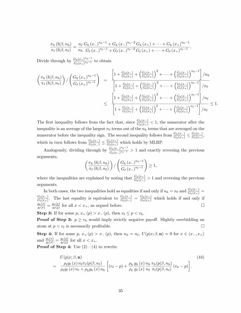
πh (b|β, nh)

π` (b|β, n`)=n`nh

Gh (x−)nh−1 +Gh (x−)nh−2Gh (x+) + · · ·+Gh (x+)nh−1

G` (x−)n`−1 +G` (x−)n`−2G` (x+) + · · ·+G` (x+)n`−1 .

Divide through by Gh(x+)nh−1

G`(x+)n`−1 to obtain

(πh (b|β, nh)

π` (b|β, n`)

)/

(Gh (x+)nh−1

G` (x+)n`−1

)=

[1 + Gh(x−)

Gh(x+) +(Gh(x−)Gh(x+)

)2+ · · ·+

(Gh(x−)Gh(x+)

)nh−1]/nh[

1 + G`(x−)G`(x+) +

(G`(x−)G`(x+)

)2+ · · ·+

(G`(x−)G`(x+)

)n`−1]/n`

≤

[1 + Gh(x−)

Gh(x+) +(Gh(x−)Gh(x+)

)2+ · · ·+

(Gh(x−)Gh(x+)

)n`−1]/n`[

1 + G`(x−)G`(x+) +

(G`(x−)G`(x+)

)2+ · · ·+

(G`(x−)G`(x+)

)n`−1]/n`

≤ 1.

The first inequality follows from the fact that, since Gh(x−)Gh(x+) < 1, the numerator after the

inequality is an average of the largest n` terms out of the nh terms that are averaged on the

numerator before the inequality sign. The second inequality follows from Gh(x−)Gh(x+) ≤

G`(x−)G`(x+) ,

which in turn follows from Gh(x−)G`(x−) ≤

Gh(x+)G`(x+) which holds by MLRP.

Analogously, dividing through by Gh(x−)nh−1

G`(x−)n`−1 > 1 and exactly reversing the previous

arguments, (πh (b|β, nh)

π` (b|β, n`)

)/

(Gh (x−)nh−1

G` (x−)n`−1

)≥ 1,

where the inequalities are explained by noting that Gh(x+)Gh(x−) > 1 and reversing the previous

arguments.

In both cases, the two inequalities hold as equalities if and only if nh = n` andGh(x−)Gh(x+) =

G`(x−)G`(x+) . The last equality is equivalent to

Gh(x−)G`(x−) = Gh(x+)

G`(x+) which holds if and only ifgh(x)g`(x) = gh(x)

g`(x) for all x < x+, as argued before. �Step 3: If for some p, x+ (p) > x− (p), then v` ≤ p < vh.

Proof of Step 3: p ≥ vh would imply strictly negative payoff. Slightly overbidding an

atom at p < v` is necessarily profitable. �Step 4: If for some p, x+ (p) > x− (p), then nh = n`, U(p|x;β,n) = 0 for x ∈ (x−, x+)

and gh(x)g`(x) = gh(x)

g`(x) for all x < x+.

Proof of Step 4: Use (2)– (4) to rewrite

U(p|x;β,n) (44)

=ρ`g` (x)n`π`(p|β, n`)

ρ`g` (x)n` + ρhgh (x)nh

[(v` − p) +

ρhρ`

gh (x)

g` (x)

nhn`

πh(p|β, nh)

π`(p|β, n`)(vh − p)

].

35

The expected payoff of a bidder with signal x ∈ (x−, x+) who bids “just above”p is

limε→0ε>0

U(p+ ε|x;β,n) (45)

=ρ`g` (x)n`G` (x+)n`−1

ρ`g` (x)n` + ρhgh (x)nh

[(v` − p) +

ρhρ`

gh (x)

g` (x)

nhn`

Gh (x+)nh−1

G` (x+)n`−1 (vh − p)].

By optimality, U(p|x;β,n) ≥ 0 for all x ∈ (x−, x+) and, by Lemma 2, G` (x+)n`−1 >

π`(p|β, n`). Therefore, it follows from (44), (45), the MLRP, Step 2 and Step 3 that

limε>0,ε→0 U(p + ε|x;β,n) ≥ U(p|x;β,n) for all x ∈ (x−, x+). The inequality is strict

if U(p|x;β,n) > 0 or nh > n` orgh(x)g`(x) > gh(x)

g`(x) for some x < x+ (or any combination).

Therefore, optimality of β implies the claim. �Step 5: If nh = n` ≥ 2 then β (x′′) = β (x′) for all x′′, x′ ∈ (x, x̂), where x̂ =

sup{x|gh(x)

g`(x) = gh(x)g`(x)

}.

Proof of Step 5: Suppose to the contrary that β (x′′) < β (x′) for some x′′, x′ ∈ (x, x̂).

Note that U(β (x) |x;β,n) = 0 in every bidding equilibrium. (If there is no atom at x, this

is immediate from the monotonicity of β; if there is an atom at x, this follows from the

Step 4.) By the choice of x̂, gh(x′)g`(x′)

= gh(x′′)g`(x′′)

= gh(x)g`(x) . This and nh = n` imply via Steps 1

and 4 that πh(β(x′′)|β,nh)π`(β(x′′)|β,n`) = πh(β(x′)|β,nh)

π`(β(x′)|β,n`) = gh(x)g`(x) . To see this, consider the second equality.

If there is no atom at β (x′), it follows from Step 1; if there is an atom, Step 4 implies

x+ (β (x′)) ≤ x̂ and it follows from Step 2. The argument for the equality between the

first and third terms is completely analogous. In addition, gh(x′′)g`(x′′)

= gh(x)g`(x) and optimality

implies U(β (x′′) |x′′;β,n) = 0. Therefore, since πω (β (x) |β, nω) > 0 for any x > x and

ω ∈ {`, h} (by monotonicity of β), evaluating (44) yields

0 = (v` − β(x′′)) +

ρhρ`

gh (x′′)

g` (x′′)

nhn`

πh(β (x′′) |β, nh)

π`(β (x′′) |β, n`)(vh − β

(x′′))

= (v` − β(x′′)) +

ρhρ`

gh (x′)

g` (x′)

nhn`

πh(β (x′) |β, nh)

π`(β (x′) |β, n`)(vh − β

(x′′))

> (v` − β(x′)) +

ρhρ`

gh (x′)

g` (x′)

nhn`

πh(β (x′) |β, nh)

π`(β (x′) |β, n`)(vh − β

(x′))

= U(β(x′)|x′;β,n),

where the second equality follows from the argument in the previous paragraph, and

the inequality follows from the hypothesis β (x′′) < β (x′). But U(β (x′) |x′;β,n) < 0

contradicts the optimality of β (x′). Therefore, β (x′′) = β (x′). �Steps 4 establishes the first part and the second item of the second part of Proposition

1; Step 5 establishes the first item of the second part.

36

9.2 Proof of Lemma 1

Proof of Lemma 1: Pr(winning bid ≤ p) =(Gω(β−1 ([0, p])

))n, where β−1 ([0, p]) =

{x : β (x) ∈ [0, p]}. Since the expectation of a positive random variable is equal to the

integral of its decumulative distribution function,

Eω [p|β, n] =

∫ vh

0

(1−

(Gω(β−1 ([0, t])

))n)dt.

Treating n as a continuous variable, dEω [p|β,n]dn2 < 0. Hence, Eω [p|β, n] is strictly concave,

which implies the lemma.

9.3 Lemmas for the Proof of Proposition 3

We state and prove an auxiliary lemma first and then three lemmas that address the

main parts of the proof. The auxiliary lemma provides a sharp relationship between the

first-order statistics in the two states (in the limit).

Lemma 3 (Poisson Approximation) Consider some sequence(xk,nk

)with min

{nk` , n

kh

}→

∞ and limnkhnk`<∞. If lim

(G`(xk))nk` = q ∈ [0, 1] then letting λ ≡ lim

nkhnk`

gh(x̄)g`(x̄) ,

lim(Gh(xk)

)nkh= qλ.

Proof of Lemma 3. Let Qω = lim(1−Gω

(xk))nkω. Observe that

lim(Gω

(xk))nkω

= lim(1−1−Gω

(xk)

nkωnkω)n

kω = e−Qω .

Since, by assumption, the limit Q` indeed exists and since lim1−Gh(xk)1−G`(xk)

nkhnk`

= λ, the limit

Qh exists as well and Qh = λQ`. Therefore, since q = e−Q` ,

lim(Gh(xk)

)nkh= e−Qh = e−λQ` = qλ.

Lemma 4 (“Zero Profit”) For any ε > 0, there is an M(ε) such that, if nω > M(ε),ω = `, h, then U(β(x)|x) < ε for all x in every bidding equilibrium β.

Proof of Lemma 4. Let ε > 0. Since, by (44), (U(b|·;β,n))b,β,n is a family of equicon-

tinuous functions, there is zε > 0 such that∣∣U(b|x′;β,n)− U(b|x;β,n)∣∣ ≤ ε

2,

for all b, all (β,n) and all x, x′ s.t. |x− x′| ≤ zε.

37

Suppose U(β(x)|x;β,n) = ε, for some x. From β being a bidding equilibrium, for all

x, x′ s.t. |x− x′| ≤ zε, ∣∣U(β(x)|x;β,n)− U(β(x′)|x′;β,n)∣∣ ≤ ε

2. (46)

Therefore, for any x,

U(β(x)|x;β,n)− ε

2≤ inf

x′∈[x−zε,x+zε]U(β(x′)|x′;β,n)

≤∑ω=`,h

ρω

∫ x+zεx−zε [vω − β(x′)]πω(β(x′)|β, nω)dGω (x′)

Gω (x+ zε)−Gω (x− zε)≤∑ω=`,h

ρωvω∫ x̄x πω(β(x′)|β, nω)dGω (x′)

Gω (x+ zε)−Gω (x− zε)

≤∑ω=`,h

ρωvωnω (Gω (x+ zε)−Gω (x− zε))

≤ E [v]

minω∈{`,h} (nω (Gω (x+ zε)−Gω (x− zε))),

where the first inequality follows from (46), the second is immediate from the definition

of U , the third owes to increasing the term in the numerator, and the fourth from the fact

that the expected probability of winning over all signals is 1/nω. Now, let M(ε) be large

enough so that, for nω ≥ M (ε), the RHS is smaller than ε2 . Therefore, for any n such

that nω ≥M (ε), U(β(x)|x;β,n) < ε.

Corollary 2 Let (nk)∞k=1 be such that min{nk` , nkh} → ∞ and (βk)∞k=1 be a correspondingsequence of bidding equilibrium strategies.(i)

lim supx∈[x,x̄]

Uk(βk(x)|x) = 0. (47)

(ii) If, for some sequence (bk)∞k=1 of bids and some ω, limπkω[bk]> 0, then for any

sequence (xk)∞k=1,limEk[v|xk,win at bk] ≤ lim bk. (48)

(iii) If limπkω[βk(xk)]> 0 for some ω sequence (xk)∞k=1, then

limβk(xk)

= limEk[v|xk,win at βk(xk)

]. (49)

Proof of Corollary 2: Part (i) and (ii) follow immediately from Lemma 4 that would

be contradicted if (47) or (48) did not hold. Part (iii) is immediate from (48) and the

individual rationality condition,

βk(xk)≤ Ek[v|xk,win at βk

(xk)

].

Lemma 5 Let nk be such that min{nk` , nkh} → ∞ and limnkhnk`

gh(x̄)g`(x̄) < 1, and let (βk)∞k=1

be a corresponding sequence of non-decreasing bidding equilibrium strategies. If (bk)∞k=1 is

38

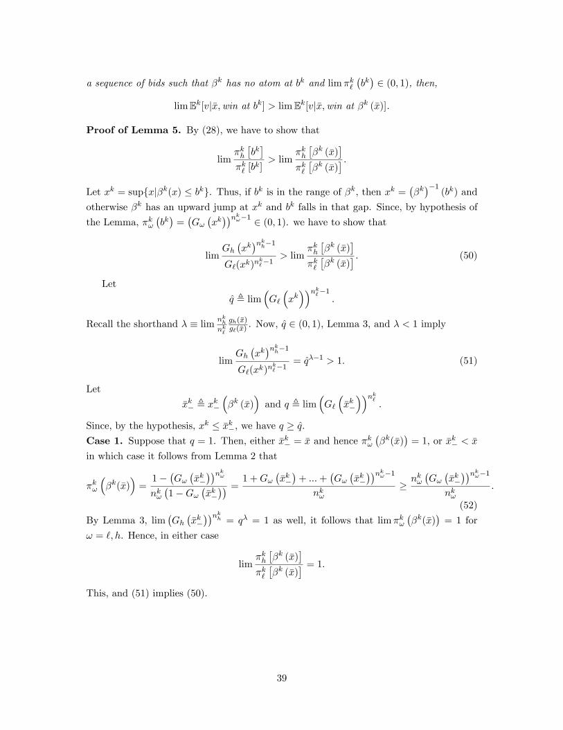
a sequence of bids such that βk has no atom at bk and limπk`(bk)∈ (0, 1), then,

limEk[v|x̄,win at bk] > limEk[v|x̄,win at βk (x̄)].

Proof of Lemma 5. By (28), we have to show that

limπkh[bk]

πk` [bk]> lim

πkh[βk (x̄)

]πk`[βk (x̄)

] .Let xk = sup{x|βk(x) ≤ bk}. Thus, if bk is in the range of βk, then xk =

(βk)−1

(bk) and

otherwise βk has an upward jump at xk and bk falls in that gap. Since, by hypothesis of

the Lemma, πkω(bk)

=(Gω(xk))nkω−1 ∈ (0, 1). we have to show that

limGh(xk)nkh−1

G`(xk)nk`−1

> limπkh[βk (x̄)

]πk`[βk (x̄)

] . (50)

Let

q̂ , lim(G`

(xk))nk`−1

.

Recall the shorthand λ ≡ limnkhnk`

gh(x̄)g`(x̄) . Now, q̂ ∈ (0, 1), Lemma 3, and λ < 1 imply

limGh(xk)nkh−1

G`(xk)nk`−1

= q̂λ−1 > 1. (51)

Let

x̄k− , xk−(βk (x̄)

)and q , lim

(G`

(x̄k−

))nk`.

Since, by the hypothesis, xk ≤ x̄k−, we have q ≥ q̂.Case 1. Suppose that q = 1. Then, either x̄k− = x̄ and hence πkω

(βk(x̄)

)= 1, or x̄k− < x̄

in which case it follows from Lemma 2 that

πkω

(βk(x̄)

)=

1−(Gω(x̄k−))nkω

nkω(1−Gω

(x̄k−)) =

1 +Gω(x̄k−)

+ ...+(Gω(x̄k−))nkω−1

nkω≥nkω(Gω(x̄k−))nkω−1

nkω.

(52)

By Lemma 3, lim(Gh(x̄k−))nkh = qλ = 1 as well, it follows that limπkω

(βk(x̄)

)= 1 for

ω = `, h. Hence, in either case

limπkh[βk (x̄)

]πk`[βk (x̄)

] = 1.

This, and (51) implies (50).

39

Case 2. Suppose that q < 1. So, there is an atom at βk(x̄). First, consider λ ∈ (0, 1).

From the first equality in (52) and from Lemma 3 and its proof,

limπk`

[βk (x̄)

]=

1− q− ln q

and limπkh

[βk (x̄)

]=

1− qλ− ln qλ

.

Hence,

limπkh[βk (x̄)

]πk`[βk (x̄)

] =

1−qλ−λ ln q

1−q− ln q

=1− qλλ (1− q) < qλ−1, (53)

where the last inequality follows from λ ∈ (0, 1), q ∈ (0, 1), and straightforward manipu-

lation.25 By the hypothesis that lim(G`(xk))nk` > 0 and xk ≤ x̄k−, we have q ≥ q̂ > 0.

This and λ < 1 imply q̂λ−1 ≥ qλ−1. Now, this together with (51) and (53) imply (50).

If λ = 0, by Lemma 3, limGh(xk)nkh = 1, and hence limπkh

[βk (x̄)

]= 1. Thus, (50)

follows from(G`(xk))nk` < πk`

[βk (x̄)

]Lemma 6 Let nk be such that min{nk` , nkh} → ∞ and lim

nkhnk`

gh(x̄)g`(x̄) > 1. Let (βk)∞k=1

be a corresponding sequence of bidding equilibria. If (βk)∞k=1 exhibits a sequence of non-

vanishing atoms (bk)∞k=1, i.e., lim(G`(xk+(bk)))nk` > lim

(G`(xk−(bk)))nk` , then

limk→∞

bk < limk→∞

limε→0

Ek[v|xk+,win at bk + ε].

Proof of Lemma 6. By bidders’individual rationality, Ek[v|xk−,win at bk] ≥ bk. There-fore, the claim will follow from Ek[v|xk+,win at bk + ε] > Ek[v|xk−,win at bk], which in turnfollows from

limgh(xk−)

g`(xk−) πkh(bk)

πk` (bk)< lim

gh(xk+)

g`(xk+) (Gh (xk+ (bk)))nkh(

G`(xk+ (bk)

))nk` . (54)

Let q− = limG`(xk−)nk` and q+ = limG`

(xk+)nk` . Note that Gω (xk+)nkω ∼= Gω

(xk+)nkω−1

for large k. By the hypothesis of the lemma, q+ > 0. By Lemma 3, limGh(xk−)nkh = (q−)λ

and limGh(xk+)nkh = (q+)λ. Recall from Lemma 2 that

limπkh(bk)

πk` (bk)

= limnk`nkh

G`(xk+)−G`

(xk−)

Gh(xk+)−Gh

(xk−)Gh (xk+)nkh −Gh (xk−)nkhG`(xk+)nk` −G` (xk−)nk` .

Using this and the above observations,

limgh(xk−)

g`(xk−) πkh(bk)

πk` (bk)

= lim

(gh(xk−)

g`(xk−) G` (xk+)−G` (xk−)Gh(xk+)−Gh

(xk−)) gh (x̄)

g` (x̄)

(q+)λ − (q−)λ

λ (q+ − q−).

25With f (q, x) = qx−1 (x+ q − xq), (53) is equivalent to f (q, x) > 1 for q, x ∈ (0, 1), which in turnfollows from f (1, x) = 1 and ∂

∂qf (·, x) = (−1) qx−2 (1− x)x (1− q) < 0 for q, x ∈ (0, 1).

40

Now, limgh(xk+)g`(xk+)

= gh(x̄)g`(x̄) and by MLRP

gh(xk−)

g`(xk−) G` (xk+)−G` (xk−)Gh(xk+)−Gh

(xk−) ≤ 1.

Therefore, we may establish (54) by showing that,

(q+)λ − (q−)λ

λ (q+ − q−)< (q+)λ−1 . (55)

Letting Q = q−q+

< 1, (55) is equivalent to Qλ − λQ + λ > 1. Since λ > 1, the LHS is

decreasing in Q over [0, 1) and is equal to 1 at Q = 1. Therefore, (55) holds and so does

(54).

9.4 Proof of Proposition 3

Proof of Proposition 3. To prove the first part, suppose limnkhnk`

gh(x̄)g`(x̄) < 1. We show

that there is a sequence(xk−, x

k+

), with xk− < xk+ such that β

k is constant on (xk−, xk+) and

lim(Gω

(xk+

))nkω − (Gω (xk−))nkω = 1 for ω ∈ {`, h} .

Consider any sequence (xk) for which lim(Gh(xk))nkh ∈ (0, 1). Let

yk− = xk−

(βk(xk))

and yk+ = xk+

(βk(xk)).

We show that

lim(Gh

(yk−

))nkh= 0 and lim

(Gh

(yk+

))nkh= 1.

In fact, it is suffi cient to prove that lim(Gh(yk+))nkh = 1, because the sequence (xk) can

be chosen to make lim(Gh(xk))nkh arbitrarily small.

Suppose to the contrary that

lim(Gh

(yk+

))nkh< 1. (56)

Then, there is some sequence of bids (bk)∞k=1 such βk has no atom at bk (i.e., either bk is

in the range of βk and xk+(bk)

= xk−(bk), or βk has an upward jump and bk falls in the

gap) and limπk`(bk)∈ (0, 1). To construct such a sequence, pick any sequence (zk)∞k=1

with zk > yk+ for all k and lim(Gh(zk))nkh = lim

(Gh(yk+))nkh . By the definition of yk+,

βk(zk)> βk

(xk). Since there are at most countably many atoms, for every k, there is

some bid bk with βk(xk)< bk < βk

(zk)such that βk has no atom at bk. Therefore,(

Gh

(yk+

))nkh ≤ πkh(bk) ≤(Gh

(zk))nkh

,

41

implying

limπkh(bk) = lim(Gh

(yk+

))nkh ∈ (0, 1) . (57)

Thus, the zero-profit condition (48) from Corollary 2 requires that

lim bk ≥ limEk[v|x̄,win at bk]. (58)

Now, since βk has no atom at bk, limnkhnk`

gh(x̄)g`(x̄) < 1, and, by (57), limπkh(bk) ∈ (0, 1), Lemma

5 implies that

limEk[v|x̄,win at bk] > limEk[v|x̄,win at βk (x̄)]. (59)

In addition, (57) and the monotonicity of βk imply that limk→∞ πkh[βk (x̄)] > 0. Therefore,

(49) from Corollary 2 requires that

limEk[v|x̄,win at βk (x̄)] = limβk (x̄) . (60)

Hence, (58)-(60) together imply

lim bk > limβk (x̄) ,

in contradiction to bk < βk(zk)and the monotonicity of βk. Thus, (56) cannot hold,

which proves the claim.

To prove the second part, suppose limnkhnk`

gh(x̄)g`(x̄) > 1 and suppose to the contrary that

βk (x) = bk for all x ∈ (xk−, xk+) and lim

(G`(xk+))nk` > lim

(G`(xk−))nk` ≥ 0. Thus,

limk→∞

limεk→0

πk`

[bk + εk

]= lim

k→∞

(G`

(xk+

))nk`> 0. (61)

This and Lemma 6 implies that

limk→∞

limεk→0

Uk(bk + εk|xk+) > 0.

contradicting the zero-profit condition (47). Thus, there can be no atom.

9.5 Proof of Proposition 6

Proof of Proposition 6: From bidders’individual rationality,

ρ` limEk[p|`] + ρh limEk[p|h] ≤ E [v] . (62)

We show that, for any p < E [v], limF kω (p) = 0. This together with (62) implies the

proposition, since if limF kω (p) < 1, for some p > E [v], (62) would be violated.

Suppose to the contrary that, for some p, limF kω (p) > 0. Therefore, there is p′ < E [v],

such that q , limπk` (p′) > 0. Then, there is a sequence

(bk)∞k=1

such that βk has no

atom at bk for any k, bk ≥ p′, and lim bk = p′. Letting q̂ , limπk` (bk), Lemma 3 and

42

λ ≡ limnkhnk`

gh(x̄)g`(x̄) = 1 imply

limπkh(bk)

πk` (bk)

=q̂λ

q̂= 1.

Thus, from (3), limEk[v|x̄,win at bk] = E [v] > lim bk. Since also limπkω(bk) > 0 from

bk > p′ and limπk` (p′) > 0, we have

limUk(bk|x̄) > 0,

contradicting the zero-profit condition (47). Thus, such(bk)∞k=1

cannot exist. Therefore,

limπkω(p) = 0 for all p < E [v], as needed.

43