A Coarse To Fine Multiscale Approach ForLinear Least Squares Optical Flow Estimation

F. Lauze1, P. Kornprobst2, E. Memin3

1. IT University of Copenhagen, Denmark,

francois@itu.dk

2. INRIA Sophia–Antipolis, France,

Pierre.Kornprobst@sophia.inria.fr

3. INRIA/IRISA University of Rennes, France,

Etienne.Memin@irisa.fr

Abstract

Tensor-based approaches for optical flow have been often criticized becauseof their limitations in handling large motions. This paper shows how to adaptthem in a multiscale coarse-to-fine strategy. We show how the same ideasused in the variational framework can be adapted by working with both amultiscale image sequence as well as a multiscale, motion compensated ten-sor field. Several experiments are presented in order to compare it to somerecent well known multiscale techniques. We demonstrate how this approachoffers a good compromise between precision and computational efficiency.

1 Introduction

Computing Optical Flow or a deformation field from a sequence of images remains acrucial problem for many applications in computer vision. In the last twenty years, a lotof improvements were made since the pioneering work of Horn and Schunck and Lucasand Kanade (see [3, 2, 16] for some reviews).

The Lucas and Kanade approach, as well as its temporal extension, is based on a leastsquares fitting of a local translational flow on a small spatial support. This approach pro-vides a very fast and local technique for motion estimation. It is in addition robust tonoise, but presents nevertheless several important drawbacks such as delocalization of oc-clusion edges, difficulty to handle very smooth areas and important motion ranges. Thesedifficulties have been quite well circumvented by hierarchical coarse-to-fine variationalmethods [1, 2, 14, 10] but at the expense of a heavy computational load.

In this paper we propose to adapt such a strategy to Lucas and Kanade-like approachesin order to handle some of the problems mentioned above. We propose to embed suchan incremental scheme into a Gaussian scale space structure of the data together with amultiscale scheme which enables us to iteratively refine the spatio-temporal estimationsupport. This strategy enables us to rely on an appropriate hierarchy of scale-space datastructure in order to estimate long displacement ranges, and to refine iteratively in a coarseto fine way the estimation support.

The paper is organized as follows: in section 2 we review some variational and Lucasand Kanade like approaches, with special focus on large scale motions. Our algorithm

is presented in section 3 and a link to the work of Nagel et al. is discussed. Section 4presents a series of experimental evaluations, followed by conclusions in section 5.

2 OFC Based Approaches And Large Motions

Let I : Ω⊂ R2×R+ → R denotes an image sequence andw = (u,v,1)T be the displace-ment vector between the frame at timet and the frame at timet +1. Most of the apparentmotion recovery algorithms start with the gray level constancy assumption, which meansthat the value of a pixel doesn’t change while moving:

I(x1 +u,x2 +v, t +1) = I(x1,x2, t). (1)

If we are considering small displacements, we can linearize (1) and obtain the optical flowconstraint (OFC) equation

w ·∇I = 0 (2)

where∇I is the 3D spatio-temporal gradient ofI . This leads to the well known apertureproblem and then additional constraints need to be considered.

2.1 Variational Approaches

One way to solve for the aperture problem is to add somea priori on the solution, suchas smoothness properties. The standard approach is to minimize an energy incorporatingthe OFC and a penalty term (some function of the gradients ofw) for the smoothness:

minw

∫

Ω(w ·∇I)2dx′1dx′2 +

∫

Ωφ(∇u,∇v)dx′1dx′2. (3)

Extensive research has been carried out in this direction, in particular to find the suitablepenalty term (see [2] for a review).

Since the OFC becomes usually not valid for large displacements, such schemes havebeen embedded into hierarchical schemes to cope with long range motion. Several differ-ent approaches have been proposed. One may distinguish multiresolution techniques [14]which rely on a multiresolution pyramid of data, scale-space approaches [1] which use ascale-space decomposition of the data and multigrid techniques [10] which explore nestedconfiguration spaces of solutions. All of these schemes rely on an incremental principlewhich consists in refining rough solutions iteratively along the levels of the consideredhierarchical structure. More precisely, assuming a known coarse estimationw of the mo-tion at a given pixel locationX = (x1,x2, t), one searches for an updatedw = (du,dv,0)T

such thatI(X +w+dw) = I(X). (4)

The linearization of the above equation provides the so-calledshiftedOFC equation:

dw ·∇wI = 0 (5)

where∇wI is theshiftedor motion compensatedgradient

∇wI =

Ix1(X +w)

Ix2(X +w)

I(X +w)− I(X)

. (6)

2.2 The Lucas and Kanade Approach

The solution proposed by Lucas and Kanade [9] consists in assuming the optical flowvector to be constant within a some neighborhood, usually a spatial or spatio-temporalGaussian window, if enough temporal information is available ([4]), defined through aGaussian kernelh, centered at the locationX = (x1,x2, t) of estimation and solve for it ina least square sense, i.e. by finding the minimizers of the local energy function

EX(w) = h∗ (∇I ·w)2(X) = wTh∗ (∇I ∇IT)

(X)w. (7)

The quantityS= S(X) = h∗ (∇I ∇IT

)(X) is by definition theStructure Tensor. The

problem to solve is thenArgminw=(u,v,1)T

EX(w) = wTSw. (8)

A minimizer w of this energy must satisfy the equation∇EX(w) = 0 which is carried outby solving the2×2 linear system

∇EX(w) =

(h∗ I2

x1h∗ Ix1

Ix2

h∗ Ix1Ix2

h∗ I2x2

)(uv

)+

(h∗ Ix1

Ith∗ Ix2

It

)= 0. (9)

These kind of approaches extract the motion from the analysis of the 2D+t structure ofthe volume which is coded in the structure tensor. The shape of the window of integrationwill determine which 2D+t structures can be successfully coded and so which motionscan be recovered. One needs to find a compromise between having a sufficiently largekernel to disambiguate the OFC and a small enough one that does not average too muchstructures. When multiple range motions have to be estimated, a common kernel for everyspeed is not satisfactory (see figure 1).

2.3 Nagel et al. Approach [13, 12, 11]

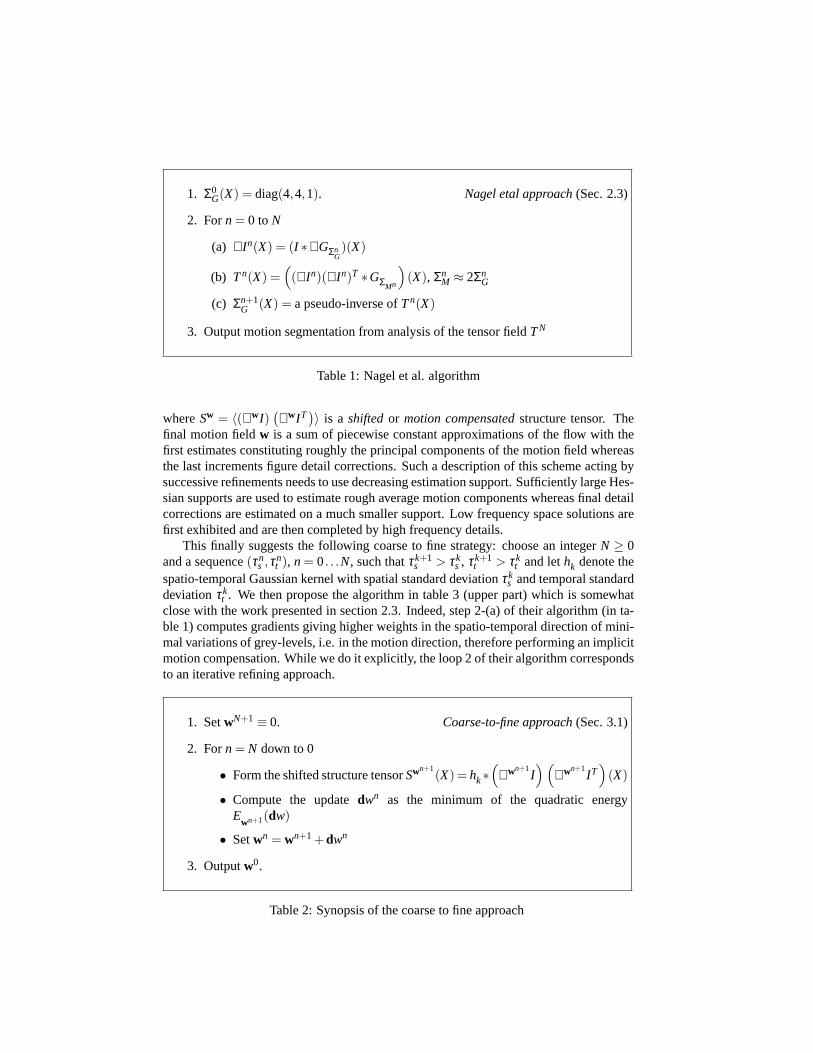
Nagelet al. have introduced a very interesting algorithm, derived of the Lucas and Kanadeapproach, that aims at segmenting the motion field in different categories. This approachcombines both image data smoothing and structure tensor smoothing. The algorithm issummarized in table 1. The pseudo-inverse operation in table 1, step 2-(c), consists inremapping in a strictly positive range the eigenvalues ofTn(X), using a bounded decreas-ing function. A major drawback of this method is its high running time due mainly to allthe convolutions with non-separable Gaussian kernels. We will see in section 3.2 that ourproposed algorithm uses, in a rough sense, a simplification of this one.

3 Using Shifted Structure Tensors

3.1 A Coarse To Fine Strategy

Within an incremental coarse-to-fine strategy (4-5), assuming the updatedw constant ona Gaussian neighborhood ofX, we can built a least squares solution atX exactly as in(8)-(9). The incremental fielddw is given at each point as the minimizer of the quadraticenergy

Ew(dw) = dwTSwdw (10)

1. Σ0G(X) = diag(4,4,1). Nagel etal approach(Sec. 2.3)

2. Forn = 0 to N

(a) ∇In(X) = (I ∗∇GΣnG)(X)

(b) Tn(X) =((∇In)(∇In)T ∗GΣMn

)(X), Σn

M ≈ 2ΣnG

(c) Σn+1G (X) = a pseudo-inverse ofTn(X)

3. Output motion segmentation from analysis of the tensor fieldTN

Table 1: Nagel et al. algorithm

whereSw = 〈(∇wI)(∇wIT

)〉 is a shiftedor motion compensatedstructure tensor. Thefinal motion fieldw is a sum of piecewise constant approximations of the flow with thefirst estimates constituting roughly the principal components of the motion field whereasthe last increments figure detail corrections. Such a description of this scheme acting bysuccessive refinements needs to use decreasing estimation support. Sufficiently large Hes-sian supports are used to estimate rough average motion components whereas final detailcorrections are estimated on a much smaller support. Low frequency space solutions arefirst exhibited and are then completed by high frequency details.

This finally suggests the following coarse to fine strategy: choose an integerN ≥ 0and a sequence(τn

s ,τnt ), n = 0. . .N, such thatτk+1

s > τks , τk+1

t > τkt and lethk denote the

spatio-temporal Gaussian kernel with spatial standard deviationτks and temporal standard

deviationτkt . We then propose the algorithm in table 3 (upper part) which is somewhat

close with the work presented in section 2.3. Indeed, step 2-(a) of their algorithm (in ta-ble 1) computes gradients giving higher weights in the spatio-temporal direction of mini-mal variations of grey-levels, i.e. in the motion direction, therefore performing an implicitmotion compensation. While we do it explicitly, the loop 2 of their algorithm correspondsto an iterative refining approach.

1. SetwN+1 ≡ 0. Coarse-to-fine approach(Sec. 3.1)

2. Forn = N down to0

• Form the shifted structure tensorSwn+1(X) = hk∗

(∇wn+1

I) (

∇wn+1IT

)(X)

• Compute the updatedwn as the minimum of the quadratic energyE

wn+1(dw)

• Setwn = wn+1 +dwn

3. Outputw0.

Table 2: Synopsis of the coarse to fine approach

1. SetwK+1,0 = 0. Multiscale coarse-to-fine approach(Sec. 3.2)

2. Fork = K downto0

(a) ComputeIk = gk ∗ I

(b) wk,N+1 = wk+1,0

(c) Forn = N downto0

• Form the shifted structure tensorSwk,n+1

(X) = hk ∗(

∇wk,n+1Ik

) (∇wk,n+1

ITk

)(X)

• Computedwk,n as the minimum of the quadratic energyEwk,n+1(dw)

• Setwk,n = wk,n+1 +dwk,n

3. Outputw0,0.

Table 3: Coarse-to-fine multiscale tensor-based motion estimation

3.2 Incorporating a Multiscale Framework

We describe here a multiscale algorithm coupling these two strategies: letK a positiveinteger, we define two family of Gaussian kernels:

• gk, k= K . . .0, with spatio-temporal standard deviations(σks ,σk

t ) so that(σks ,σk

t ) >

(σk−1s ,σk−1

t ). This will be used to smooth of the image data.

• hkn, k = K . . .0, n = N . . .0, with standard spatio-temporal deviations(τk,ns ,τk,n

t )such that(τk,n

s ,τk,nt ) > (τk,n−1

s ,τk,n−1t ). This will be used for the least squares esti-

mates of the motion update vectors.

We also require that(τk,0s ,τk,0

t ) À (σks ,σk

t ) which states that the minimal aperture at agiven image scale for forming the structure tensors must be sufficiently larger than the oneused to smooth the image data, otherwise the extracted gradients will be too well alignedin the chosen neighborhood, and we might be in presence of the aperture problem.

This algorithm is shown in table 3. Standard central differences are used for thespatial derivatives, and Gaussian filtering is approximated by Deriche recursive filters[7]. In order to compute the valuesI(X +w) we use bilinear interpolation. The standarddeviation sequences used are exponential: givenα > 1, βk > 1, we set

(σks ,σk

t ) = αk(σ0s ,σ0

t ), (τk,ns ,τk,n

t ) = β nk (τk,0

s ,τk,0t ).

4 Experiments

Our algorithm has been implemented in C++ on a 1.6Ghz Pentium IV processor. In allexperiments but the last, we have usedK = N = 3,σ0

s = 1.0,σ0s = 0.5,τk,0

s = 3.0,τk,0t =

1.5,α = βk =√

2. Interestingly the approach is not so sensitive to changes in the pyramids

levels (as soon as we start from coarse enough scale) which is an advantage with respectto multiresolution schemes that can lead to quite different results with different scales.

The proposed method, denoted CFLS (Coarse to Fine Least Squares) is comparedwith the new variational algorithm by Broxet. al. [5] (denoted BBPW), which providessome of the best results known so far, and with the multiscale variational approach byAubertet. al. [2] (denoted ADK).

We first comment some experiments using several synthetic image sequences wherethe ground truth is known. The following measurements have been estimated (see [3]):AAE (the average angular error), AESTD (the angular error standard deviation), ANE(the average norm error) and NESTD (norm error standard deviation), RT (running time).

Different aspects have been evaluated. In addition, we have computed orientationimages, for some of the sequences, the orientation represented by a color, and the usedcolor code is indicated by a small band at the image boundary.

(a) The ability to recover a large range of motions(Figures 1 and 2). This sequenceconsists of five stacked translating patterns at different speeds (20, 13, 7, 4 and 2 pixelsper frame leftward). Figure 1-(a) shows one frame of the sequence, 1-(b) the true flow and1-(c) shows that using the original Lucas and Kanade approach with several homogeneousGaussian kernels doesn’t allow to recover the different ranges of motions and discontinu-ities. The graph in figure 2-(a) and the table 2-(c) allow to compare the different methods.BBPW is clearly better as shown in figure 2-(a), which represents a vertical cut of thevelocities forx = 34. Figure 2-(b) illustrates the refining behavior of estimations in ouralgorithm (locations indicated by the spots in figure 1-(a)).

(b) Robustness to noise(Figure 3). This sequence is of dimensions 170×255×20pixels, has a leftward 10 pixels per frames motion, but is heavily contaminated by nonstationnary noise: the frames are divided in 3 rectangles with Gaussian noise of stan-dard deviation 35% for the upper one, 58% for the middle one and 86% for the bottomone. Figure 3)-(b) is the true flow, and figure 3)-(c) shows very good computed motionorientations, although severe errors (overestimates) are present at the left boundary.

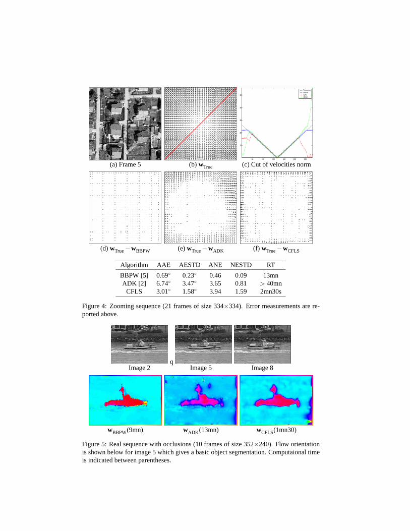
(c) Dealing with diverging motions (Figure 4). This sequence is a zoom in, withrespect to the image center. Figure 4-(b) represents the true flow and figure 4-(c) repre-sents velocity norms cuts for the red diagonal of figure 4-(b). Figure 4-(d),(e),(f) comparethe true flow to the ones computed using respectively BBWP, ADK and our method. Wecapture reasonably the motion range and runs much faster than BBPW and ADK.

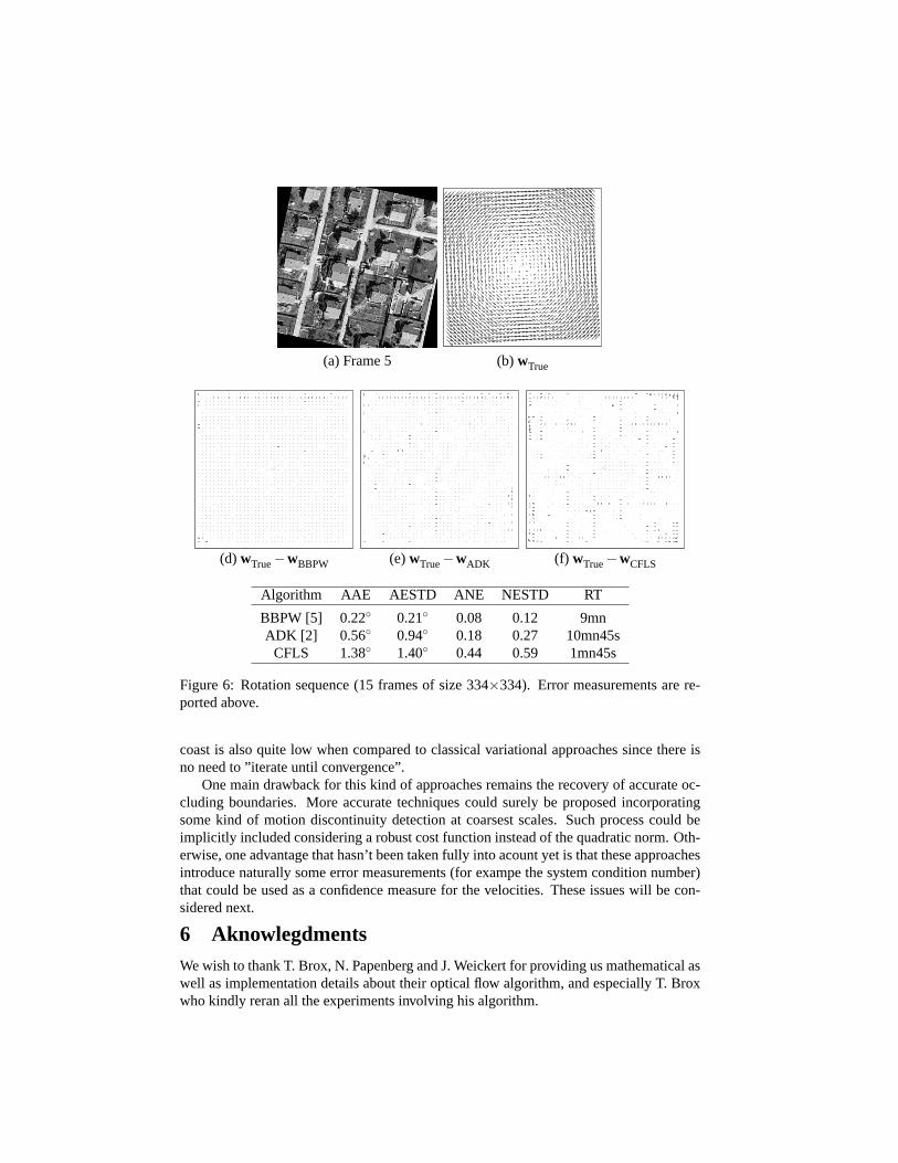
(d) Dealing with rotational motions (Figure 6). This sequence is a 4 counterclock-wise rotation, with respect to the image center. Figure 6-(b) represents the true flow. Fig-ure 6-(c),(d),(e) compare the true flow to the ones computed using respectively BBWP,ADK and our method. BBPW returns the best results, ADK gives also very good results,and our algorithm is a bit less accurate but much faster.

(e) Recovering motion with occlusions(Figure 5). This real sequence shows a boatmoving slighly to the right while the background is moving leftward. Although the twovariational methods BBWP and ADK give slightly better edges, we are able capture cor-rectly the two motions.

5 Conclusion

This paper demonstrates that a linear tensor-based approach can be successfully extendedin a multiscale framework and estimate high range velocities robustly. The computational

50 100 150 200 250 300 350 4002

4

6

8

10

12

14

16

18

20

True motionSmall aperturesMedium aperturesLarge apertures

(a) One image (b)wTrue (c) Lucas and Kanade with differentσ

Figure 1: Multispeed sequence (21 frames of size 170×425)

50 100 150 200 250 300 350 4002

4

6

8

10

12

14

16

18

20True motionBBPWADKCFLS

K=3 K=2 K=1 K=0

5

10

15

20

25 y=42y=127y=212y=297y=382True norms

(a) (b)

(c)

Algorithm AAE AESTD ANE NESTD RT

BBPW [5] 0.67 0.81 0.30 0.14 17mnADK [2] 1.37 1.02 0.51 0.15 11mn40s

CFLS 1.43 0.62 1.60 2.90 1mn35s

Figure 2: Multispeed sequence: (a) Vertical cuts of the velocitiy norms, (b) evolution ofvelocities across scales, at positionx = 85, t = 4 andy as shown in figure 1, (c) errormeasurements.

(a) frame 4 (b)wTrue (c) Orientations computed (d)wTrue−wCFLS

Figure 3: Robustness to noise (21 frames of size 170×255). Error measurements arerespectively AAE = 1.65, AESTD = 0.62, ANE = 2.20, NESTD = 0.62.

50 100 150 200 250 300

10

20

30

40

50

True normBBPWADKCFLS

(a) Frame 5 (b)wTrue (c) Cut of velocities norm

(d) wTrue−wBBPW (e)wTrue−wADK (f) wTrue−wCFLS

Algorithm AAE AESTD ANE NESTD RT

BBPW [5] 0.69 0.23 0.46 0.09 13mnADK [2] 6.74 3.47 3.65 0.81 > 40mn

CFLS 3.01 1.58 3.94 1.59 2mn30s

Figure 4: Zooming sequence (21 frames of size 334×334). Error measurements are re-ported above.

qImage 2 Image 5 Image 8

wBBPW(9mn) wADK (13mn) wCFLS(1mn30)

Figure 5: Real sequence with occlusions (10 frames of size 352×240). Flow orientationis shown below for image 5 which gives a basic object segmentation. Computaional timeis indicated between parentheses.

(a) Frame 5 (b)wTrue

(d) wTrue−wBBPW (e)wTrue−wADK (f) wTrue−wCFLS

Algorithm AAE AESTD ANE NESTD RT

BBPW [5] 0.22 0.21 0.08 0.12 9mnADK [2] 0.56 0.94 0.18 0.27 10mn45s

CFLS 1.38 1.40 0.44 0.59 1mn45s

Figure 6: Rotation sequence (15 frames of size 334×334). Error measurements are re-ported above.

coast is also quite low when compared to classical variational approaches since there isno need to ”iterate until convergence”.

One main drawback for this kind of approaches remains the recovery of accurate oc-cluding boundaries. More accurate techniques could surely be proposed incorporatingsome kind of motion discontinuity detection at coarsest scales. Such process could beimplicitly included considering a robust cost function instead of the quadratic norm. Oth-erwise, one advantage that hasn’t been taken fully into acount yet is that these approachesintroduce naturally some error measurements (for exampe the system condition number)that could be used as a confidence measure for the velocities. These issues will be con-sidered next.

6 AknowlegdmentsWe wish to thank T. Brox, N. Papenberg and J. Weickert for providing us mathematical aswell as implementation details about their optical flow algorithm, and especially T. Broxwho kindly reran all the experiments involving his algorithm.

References[1] L. Alvarez, J. Weickert, and J. Sanchez. Reliable estimation of dense optical flow

fields with large displacements.The International Journal of Computer Vision,39(1):41–56, August 2000.

[2] G. Aubert, R. Deriche, and P. Kornprobst. Computing optical flow via variationaltechniques.SIAM Journal of Applied Mathematics, 60(1):156–182, 1999.

[3] J.L. Barron, D.J. Fleet, and S.S. Beauchemin. Performance of optical flow tech-niques.The International Journal of Computer Vision, 12(1):43–77, 1994.

[4] J. Bigun, G. H. Granlund, and J. Wiklund. Multidimensional orientation estima-tion with applications to texture analysis and optical flow.IEEE Transactions onPattern Analysis and Machine Intelligence, 13(8):775–790, August 1991. ReportLiTH-ISY-I-0828 1986 and Report LiTH-ISY-I-1148 1990, both at Computer Vi-sion Laboratory, Linkoping University, Sweden.

[5] T. Brox, A. Bruhn, N. Papenberg, and J. Weickert. High accuracy optical flow esti-mation based on a theory for warping. In T. Pajdla and J. Matas, editors,Proceedingsof the 8th European Conference on Computer Vision, Prague, Czech Republic, 2004.Springer–Verlag.

[6] T. Brox and J. Weickert. Nonlinear matrix diffusion for optic flow estimation. InDAGM-Symposium, pages 446–453, 2002.

[7] R. Deriche. Fast algorithms for low-level vision.IEEE Transactions on PatternAnalysis and Machine Intelligence, 1(12):78–88, January 1990.

[8] F. Lauze, P. Kornprobst, C. Lenglet, R. Deriche, and M. Nielsen. Sur quelquesmethodes de calcul de flot optiquea partir du tenseur de structure : Synthese etcontribution. In14eme Congres Francophone AFRIF-AFIA de Reconnaissance desFormes et Intelligence Artificielle, 2004.

[9] B. Lucas and T. Kanade. An iterative image registration technique with an appli-cation to stereo vision. InInternational Joint Conference on Artificial Intelligence,pages 674–679, 1981.

[10] E. Memin and P. Perez. Hierarchical estimation and segmentation of dense motionfields. The International Journal of Computer Vision, 46(2):129–155, 2002.

[11] M. Middendorf and H.-H. Nagel. Estimation and interpretation of discontinuities inoptical flow fields. InProceedings of the 8th International Conference on ComputerVision, pages 178–183.

[12] M. Middendorf and H.-H. Nagel. Empirically convergent adaptive estimation ofgrayvalue structure tensors. InDAGM-Symposium, pages 66–74, 2002.

[13] H.-H. Nagel and A. Gehrke. Spatiotemporally adaptive estimation and segmentationof OF-fields. In Hans Burkhardt and Bernd Neumann, editors,Proceedings of the 5thEuropean Conference on Computer Vision, volume 2 ofLecture Notes in ComputerScience, pages 86–102, Freiburg, Germany, June 1998. Springer–Verlag.

[14] H.H. Nagel and W. Enkelmann. An investigation of smoothness constraint for theestimation of displacement vector fields from image sequences.IEEE Transactionson Pattern Analysis and Machine Intelligence, 8:565–593, 1986.

[15] H. Spies and H. Scharr. Accurate optical flow in noisy image sequences. InPro-ceedings of the 8th International Conference on Computer Vision, pages 587–592.

[16] J. Weickert and C. Schnorr. A theoretical framework for convex regularizers in pde-based computation of image motion.The International Journal of Computer Vision,45(3):245–264, December 2001.