Nova Southeastern UniversityNSUWorks

HCNSO Student Theses and Dissertations HCNSO Student Work

3-1-2015

A Catch Per Unit Effort (CPUE) Spatial Metricwith Respect to the Western North Atlantic PelagicLongline FisheryMax AppelmanNova Southeastern University, ma1177@nova.edu

Follow this and additional works at: https://nsuworks.nova.edu/occ_stuetd

Part of the Marine Biology Commons, and the Oceanography and Atmospheric Sciences andMeteorology Commons

Share Feedback About This Item

This Thesis is brought to you by the HCNSO Student Work at NSUWorks. It has been accepted for inclusion in HCNSO Student Theses andDissertations by an authorized administrator of NSUWorks. For more information, please contact nsuworks@nova.edu.

NSUWorks CitationMax Appelman. 2015. A Catch Per Unit Effort (CPUE) Spatial Metric with Respect to the Western North Atlantic Pelagic Longline Fishery.Master's thesis. Nova Southeastern University. Retrieved from NSUWorks, Oceanographic Center. (36)https://nsuworks.nova.edu/occ_stuetd/36.

NOVA SOUTHEASTERN UNIVERSITY OCEANOGRAPHIC CENTER

A CATCH PER UNIT EFFORT (CPUE) SPATIAL METRIC WITH RESPECT TO

THE WESTERN NORTH ATLANTIC PELAGIC LONGLINE FISHERY

By

Max H. Appelman

A Thesis

Submitted to the Faculty of

Nova Southeastern University Oceanographic Center

In partial fulfillment of the requirements for

The degree of Master of Science with a specialty in:

Marine Biology and

Coastal Zone Management

March 2015

Thesis of

Max H. Appelman

Submitted in Partial Fulfillment of the Requirements for the Degree of

Master of Science:

Marine Biology

and

Coastal Zone Management

Nova Southeastern University

Oceanographic Center

March 2015

Thesis Committee

Major Professor: __________________________________

David Kerstetter, Ph.D.

Committee Member: _______________________________

Brian Walker, Ph.D.

Committee Member: _______________________________

Bernhard Riegl, Ph.D.

iii

Table of Contents Page

Acknowledgements IV

List of Tables V

List of Figures VI

Abstract VIII

Introduction 1

Characterizing pelagic longline gear 2

Highly migratory species management and the western North Atlantic pelagic

longline fishery 5

Catch per unit effort: abundance estimates and stock assessments 9

Spatial CPUE abundance indices 14

Materials and Methods 23

Data collection 23

Deriving spatially CPUE 26

Statistical analysis 26

Non-spatial statistical analysis and PAF 26

Hot spot analysis 28

Results 33

Non-spatial statistics 33

Spatial statistics 47

Discussion 55

Non-spatial analyses 55

Optimized hot spot analysis 56

Spatial analysis by management zone 57

Temporal analysis 75

Comparing SCPUE to other spatial-CPUE metrics 98

Management implications: stock assessments, essential fish habitat and

areas of particular concern 100

Conclusion and future research 101

Works cited 104

Appendix 109

iv

Acknowledgments

Special thanks to Dave Kerstetter, my advisor, employer and mentor for sharing

his passion and knowledge of marine fisheries with me. I am grateful for the invaluable

experiences he has provided me at Nova Southeastern University’s Oceanographic

Center’s Fisheries Research Laboratory, which has undoubtedly formed the foundation of

my future career in marine fisheries. Thank you to my committee members Dr. Bernhard

Riegl and Dr. Brian Walker for their knowledge, expertise, and mentorship throughout

my academic career at NSU’s Oceanographic Center. A special thank you to all of the at-

sea observers from NSU’s Fisheries Lab and the National Marine Fisheries Service for

collecting the catch and effort date used in this study. Thank you to all of the

participating vessels for their time and cooperation, without which research like this

would not be possible. Also, I’d like to acknowledge and thank all of my current and

former NSU OC Fisheries Lab-mates who provided insight and encouragement,

especially Matt Dancho, Sohail Khamesi and Jesse Secord.

v

Tables Page

1. U.S. Atlantic pelagic longline observer coverage 8

2. Spatially-based CPUE results: bottom trawl shrimp fishery (Can et al. 2004) 18

3. Species by name and code 25

4. Target species: number of sets by year 37

5. Total animals: number by species and year 39

6. Total effort by year 40

7. Perceived Area Fished (PAF) T-test results 41

8. PAF distribution results 42

9. ANOVA results: SCPUE 45

10. T-test results: SCPUE via different PAF methods 46

11. Hot spot areas for aggregated dataset 48

12. Hot spot areas for 2008-2010 subset 49

vi

Figures Page

1. Diagram of pelagic longline (PLL) gear 4

2. Relationship between CPUE and stock abundance 12

3. Management zones of the U.S. Atlantic pelagic longline fishery 13

4. Spatio-temporal distribution of pelagic longline fishing in the North Atlantic 17

5. 2006 PLL Take Reduction Plan : marine mammal interactions 21

6. 2011 ICCAT yellowfin tuna stock assessment: catch distribution 22

7. Perceived area fished (PAF) methods diagram 30

8. (A) ArcGIS screen shot: 2 km buffer 31

(B) ArcGIS screen shot: minimum convex polygons 32

9. (A) observed PLL sets from the aggregated data set 35

(B) observed PLL sets from the 2008-2010 subset 36

10. Percent target species 38

11. (A) CPUE histogram 43

(B) SCPUE histogram 44

12. Fishing effort optimized hot spot analysis for aggregated data set 50

13. (A) SCPUE optimized hot spot analysis for retained swordfish 51

(B) CPUE optimized hot spot analysis for retained swordfish 52

14. (A) SCPUE optimized hot spot analysis for billfish 53

(B) CPUE optimized hot spot analysis for billfish 54

15. CPUE optimized hot spot analysis for retained swordfish in the South

Atlantic Bight and Florida East Coast 58

16. SCPUE optimized hot spot analysis for retained swordfish in the South

Atlantic Bight and Florida East Coast 59

17. CPUE optimized hot spot analysis for billfish in the South Atlantic

Bight and Florida East Coast 62

18. SCPUE optimized hot spot analysis for billfish in the South Atlantic

Bight and Florida East Coast 63

19. CPUE optimized hot spot analysis for retained swordfish in the Gulf of Mexico 66

20. SCPUE optimized hot spot analysis for retained swordfish in the Gulf of Mexico 67

21. CPUE optimized hot spot analysis for billfish in the Gulf of Mexico 68

vii

22. SCPUE optimized hot spot analysis for billfish in the Gulf of Mexico 69

23. CPUE optimized hot spot analysis for billfish in the Mid Atlantic Bight and

Northeast Coastal 71

24. SCPUE optimized hot spot analysis for billfish in the Mid Atlantic Bight and

Northeast Coastal 72

25. CPUE optimized hot spot analysis for retained swordfish in the Mid Atlantic

Bight and Northeast Coastal 73

26. SCPUE optimized hot spot analysis for retained swordfish in the Mid Atlantic

Bight and Northeast Coastal 74

27. Fishing effort optimized hot spot analysis from the 2008-2010 subset 76

28. CPUE optimized hot spot analysis for retained swordfish

from the 2008-2010 subset 77

29. SCPUE optimized hot spot analysis for retained swordfish

from the 2008-2010 subset 78

30. CPUE optimized hot spot analysis of for billfish from the 2008-2010 subset 79

31. SCPUE optimized hot spot analysis of for billfish from the 2008-2010 subset 80

32. (A) 2008 fishing effort optimized hot spot analysis 82

(B) 2009 fishing effort optimized hot spot analysis 83

(C) 2010 fishing effort optimized hot spot analysis 84

33. (A) 2008 optimized hot spot analysis of CPUE for billfish 85

(B) 2009 optimized hot spot analysis of CPUE for billfish 86

(C) 2009 optimized hot spot analysis of CPUE for billfish 87

34. (A) 2008 optimized hot spot analysis of spatial CPUE for billfish 88

(B) 2009 optimized hot spot analysis of spatial CPUE for billfish 89

(C) 2010 optimized hot spot analysis of spatial CPUE for billfish 90

35. (A) 2008 optimized hot spot analysis of CPUE for retained swordfish 91

(B) 2009 optimized hot spot analysis of CPUE for retained swordfish 92

(C) 2010 optimized hot spot analysis of CPUE for retained swordfish 93

36. (A) 2008 optimized hot spot analysis of spatial CPUE for retained swordfish 95

(B) 2009 optimized hot spot analysis of spatial CPUE for retained swordfish 96

(C) 2010 optimized hot spot analysis of spatial CPUE for retained swordfish 97

viii

Abstract

Catch per unit effort (CPUE) is a quantitative method used to describe fisheries

worldwide. CPUE can be presented as number of fish per 1000 hooks, number of fish

per amount of fishing time, or with any unit of effort that best describes the fishery (e.g.,

search time, hooks per hour, number of trawls). CPUE is commonly used as an index to

estimate relative abundance for a population. These indices are then applied within stock

assessments so that fisheries managers can make justified decisions for how to manage a

particular stock or fishery using options such as quotas, catch limitations, gear and

license restrictions, or closed areas. For commercial pelagic longline (PLL) fisheries,

onboard observer data are considered the only reliable data available due to the large-

scale movements of highly migratory species (HMS) like tunas and because of the high

costs associated with fisheries independent surveys. Unfortunately, fishery-reported

logbook data are heavily biased in favor of the target species and the expense of onboard

observers results in a low percentage of fleet coverage. Subsequently, CPUE derived

from fishery-dependent data tends to overestimate relative abundance for highly

migratory species. The spatial distribution of fish and fishing effort is essential for

understanding the proportionality between CPUE and stock abundance. A spatial metric

was created (SCPUE) for individual gear deployments using observer-based catch and

effort data from the western North Atlantic PLL fleet. SCPUE was found to be less

variable than CPUE when used as an index of relative abundance, suggesting that SCPUE

could serve as an improved index of relative abundance within stock assessments because

it explicitly incorporates spatial information obtained directly from the fishing location.

Areas of concentrated fishing effort and fine-scale aggregations of target and non-target

fishes were identified using the optimized hot spot analysis tool in ArcGIS (10.2). This

SCPUE method describes particular areas of fishing activity in terms of localized fish

density, thus eliminating the assumption that all fish in a population are dispersed evenly

within statistical management zones. The SCPUE metric could also assist fisheries

management by identifying particular areas of concern for HMS and delineating

boundaries for time-area closures, marine protected areas, and essential fish habitat.

Keywords: CPUE, pelagic longline, relative abundance, spatial distribution

1

Introduction

Catch per unit effort (CPUE) is a statistical method used to quantify the number

of fish caught per unit of effort for a commercial fishing activity (Harley et al. 2001).

CPUE can be represented as number of fish per 1000 hooks (the metric used for pelagic

longline fisheries), number of fish per amount of fishing time (commonly used in trawl

fisheries), or with any other unit of effort that best describes the gear type and the fishery

(e.g., search time, number of hooks per hour, number of trawls, number of fish per square

kilometer). CPUE is commonly used as an index to estimate relative abundance of a

population (Harley et al. 2001, Maunder et al. 2006, and Lynch et al. 2012). Fisheries

scientists take these indices of relative abundance and apply them within stock

assessment models, which are then used by fisheries managers and policymakers to make

justified decisions of how to manage a particular stock or fishery. Management actions

are frequently expressed via a combination of catch quotas, catch limits, license

restrictions and limitations, gear restrictions or modifications, and time-area closures

often resulting in economic repercussions affecting the fishermen and consumers alike

(Maunder et al. 2006).

Abundance estimates can only be as accurate as the data behind them, and CPUE

has frequently been misinterpreted, resulting in relatively poor managerial decisions. A

classic example is the collapse of the northwest Atlantic cod Gadus morhua in the late

1980s. Cod exhibit increasing schooling behavior as population decreases (Hutchings

1996). Because of this schooling behavior, consistently high CPUEs were maintained by

bottom trawlers in this region from the 1960s through the mid-1980s, even though the

stock was declining exponentially. Ultimately, the cod population was fished so low that

the stock crashed and the North Atlantic U.S. commercial cod fishery closed in 1992

(Hutchings 1996). In this example, northwest Atlantic cod CPUE was disproportionately

high in relation to stock abundance. Catch, essentially, can only be proportional to

abundance if the catchability of all individuals in a population is constant. Since

catchability is rarely constant throughout a population, raw CPUE is rarely proportional

to abundance (Maunder et al. 2006). Variables effecting catchability include changes in

fleet efficiency or fleet dynamics (Gillis and Peterman 1998), changes in target species,

spatial and temporal effects (Nishida and Chen 2004) and most prominently, interactions

2

between the fishing method and the target species population dynamics (Maunder et al.

2006). Specifically, fisheries dependent CPUE data only come from areas in which a

fishery operates, providing no information on other areas inhabited by the target stock

(Walters 2003). It is very common for a fishery to operate on only a fraction of a

population’s geographic range, especially for highly migratory species like tunnid tunas

and swordfish Xiphias gladius. If non-fished areas are not addressed explicitly within

CPUE analyses, then in the context of fisheries management, they are assumed to have

the same characteristics (e.g., population abundance) as the fished areas. This oversight

can lead to severely inaccurate abundance indices and subsequent poor management

regimes (Walters 2003). Abundance estimates for commercially valued pelagic species

like swordfish rely heavily on pelagic longline CPUE data, and these estimates usually do

not explicitly incorporate spatial analysis.

Characterizing pelagic longlines

Pelagic longline (PLL) gear is a commercial fish harvesting method that primarily

targets species that undergo transoceanic seasonal migrations commonly referred to as

highly migratory species (HMS) (FSEIC 1999). The PLL fishery in the western North

Atlantic (WNA) primarily targets swordfish, yellowfin tuna Thunnus albacares, and

bigeye tuna Thunnus obesus; however, other oceanic species (e.g., selected shark species

and common dolphinfish Coryphaena hippurus) are targeted during various seasons

(SAFE 2014). Modern PLL gear (Figure 1) typically consists of 20-30 miles of heavy

monofilament mainline with baited drop lines, or gangions, attached at predetermined

increments along the mainline (Watson and Kerstetter 2006). Using the appropriate

combination of buoys and weights, fishermen deploy PLL gear from just below the sea

surface to 350 m depths and leave the gear to passively fish (referred to as “soak time”)

for several hours to overnight before the gear is retrieved. Typically, a PLL set is

deployed in standardized sections. Each section is marked with a high-flyer, usually

equipped with a strobe light (and sometimes with GPS devices), to aid tracking of the

gear during the soak, and to warn vessels of its presence.

PLL practices have been documented since the mid 1800’s; the gear type was

initially developed in Japanese fisheries to target Pacific bluefin tuna Thunnus orientalis

3

and then expanded eastward to the United States and other nations in the early 20th

century (Watson and Kerstetter 2006). Improvements in fishing technology have

increased the efficiency of PLL gear over the decades. For example, the introduction of

diesel-powered engines in the 1920s coupled with the introduction of freezer vessels in

the 1950s allowed vessels to follow the target species’ large-scale movements and remain

on the fishing grounds longer (Watson and Kerstetter 2006; Ward and Hindmarsh 2007).

The switch from iron hooks to high-carbon and stainless steel hooks in the 1950s and the

introduction of a single-strand polyamide monofilament mainline in the 1970s (Watson

and Kerstetter 2006) increased catchability by reducing the rates of fish loss (Ward and

Hindmarsh 2007). The introduction of electronic devices, including GPS, radars, echo

sounders, electric powered bandit reels, and computer- and satellite-aided data acquisition

of current profiles, sea surface temperature, atmospheric patterns, and ocean bathymetry

have also vastly increased PLL efficiency via enhanced navigation, communication, and

ability to find target populations (Watson and Kerstetter 2006).

PLL fishermen are opportunistic and regularly modify gear configurations to

target the most profitable species with each individual trip (SAFE 2014). Consequently,

PLL gear is relatively non-selective and frequently interacts with bycatch species (i.e.,

non-target species), including protected sea turtles, marine mammals, and some seabird

and shark species (SAFE 2014). Due to federal regulations, PLL fishermen are

prohibited from landing these bycatch species and they are often discarded, whether alive

or dead (HMS FMP 2006). Increased awareness of associated problems with high PLL

bycatch (NOAA 2012) has enticed the development of gear technologies to reduce

bycatch in PLL operations (Watson and Kerstetter 2006). Gear introductions include

tori-lines and lineshooters to reduce seabird bycatch (Melvin 2000), circle hooks to

reduce incidental catch of sea turtles, and “weak hooks” that allow much larger marine

animals (e.g., porpoises, sharks, “giant” bluefin tuna) to bend the hook and thereby

release themselves (Bigelow et al. 2012). Still further, altering operating characteristics

including geographic area, month and time of fishing, fishing depth, and length of soak

time can also increase the selectivity – and ultimately the sustainability – of PLL gear-

based fisheries (Hoey and Moore 1999).

4

Figure 1. Diagram of modern (monofilament) pelagic longline gear. Not depicted to

scale. Retrieved via: http://www.nmfs.noaa.gov

5

HMS Management and the WNA PLL Fishery

Management of the WNA PLL tuna fishery is relatively new compared to other

natural resources. First enacted in 1976 as the Fishery Conservation and Management

Act, the Magnuson-Stevens Fishery Conservation and Management Act (MSA) is the

“primary law governing marine fisheries management in United States federal waters”

(MSA 1996). At that time, the United States claimed ownership of marine territory from

the coastline out to 200 nautical miles, thereby prohibiting foreign fleets from these

waters (commonly referred to as the Exclusive Economic Zone, or EEZ). In 1990, after

unsuccessful management by several coordinated U.S. regional fishery management

councils, the Fishery Conservation Amendments gave the U.S. Secretary of Commerce

authority to manage tunas in the U.S. EEZ (as well as other HMS in the Atlantic Ocean,

Gulf of Mexico, and Caribbean Sea) under the MSA (HMS FMP 2006). The Secretary of

Commerce, at that time, delegated authority of Atlantic HMS to the National Marine

Fisheries Service (NMFS). The HMS Management Division, which manages and

regulates all Atlantic HMS fisheries within the United States, was then created by NMFS

(HMS MD 2014). The 1990 amendment also defined HMS to be marlin (Tetrapturus

spp. and Makaira spp.), oceanic sharks, sailfishes (Istiophorus spp.), swordfish Xiphias

gladius, and tuna species; including “BAYS” tunas (bigeye tuna Thunnus obesus,

albacore tuna Thunnus alalunga, yellowfin tuna Thunnus albacares, and skipjack tuna

Katsuwonus pelamis), and Atlantic bluefin tuna Thunnus thynnus.

The MSA was amended several times over the following years. Most notably, the

MSA was amended with the Sustainable Fisheries Act (SFA) in 1996 requiring NMFS to

create advisory panels (APs) to help develop fisheries management plans (FMPs) for

Atlantic HMS (HMS MD 2014). The 1996 amendments focus on rebuilding over-fished

fisheries, protecting essential fish habitat, and reducing bycatch. Per the SFA, the

management of Atlantic HMS fisheries must also be consistent with other regulations

such as the Marine Mammal Protection Act, the Endangered Species Act, the Migratory

Bird Treaty Act, the National Environmental Policy Act, the Coastal Zone Management

Act, and other Federal laws (HMS MD 2014).

However, fisheries management organizations acknowledged that new strategies

had to be adopted in order to ensure the viability of U.S. marine fisheries. Thus, the

6

MSA was amended yet again in 2006 and re-named the Magnuson-Stevens Fishery

Conservation and Management Reauthorization Act (MSRA). In essence, the MSRA

continues to promote sustainable fisheries by: 1) mandating that regional fisheries

management councils (of the U.S. Secretary of Commerce) end over-fishing; 2)

stemming illegal, unregulated and unreported fishing (IUU fishing); 3) improving

NOAA’s fisheries science programs via enhanced fisheries monitoring protocols, and; 4)

increase market-based management programs such as Limited Access Privilege Programs

which, through catch-share allocations, promotes fishermen safety and economic viability

of the fishery (MSRA 2008).

The management of U.S. Atlantic HMS fisheries is also governed by the Atlantic

Tuna Convention Act (1975), which recognizes the need for international cooperation

and mandates NMFS to implement domestically any management recommendations

agreed upon by the International Commission for the Conservation of Atlantic Tunas

(ICCAT) (HMS FMP 2014). Established in 1966, ICCAT is dedicated to the Atlantic-

wide sustainable management of HMS. The organization also requires all member

nations to collect scientifically sound catch and effort data, and to make that those data

available to the Commission (ICCAT 2013). Each year, fisheries scientists from ICCAT

members conduct stock assessments for most regulated Atlantic HMS in October, then

the member nations meet in November to negotiate quotas and management

recommendations based on these stock assessments. If these recommendations are

adopted by ICCAT, then the United States must enforce them. Among the many

international management bodies that could affect Atlantic HMS management [i.e.,

Convention on International Trade in Endangered Species of Wild Fauna and Flora

(CITES), the Food and Agriculture Organization of the United Nations (FAO) and

International Plan of Action for the Conservation and Management of Sharks (IPOA-

Sharks)], ICCAT is the most significant (HMS MD 2014).

Current management and regulations for Atlantic HMS can be found in the Code

of Federal Regulations (title 50, chapter 6, parts 600-659). All management measures are

detailed pertaining to each species defined by the HMS Management Division, and for

each fish harvesting method that may effect the management of those species (e.g.,

demersal longlines, greenstick gear, swordfish buoy gear, pelagic longline gear, seines).

7

Aside from required vessel permits, fishery access restrictions, and gear identification,

the most notable Atlantic HMS management measures include size limits, catch quotas,

gear and deployment restrictions, commercial retention limits, time-area closures, and

possession and sales restrictions (e-CFR 2013). In 1992, the Southeast Fisheries Science

Center (SEFSC), one of six regional science centers operating under the direction of

NMFS, launched the Pelagic Observer Program (POP). Although NMFS has used

contracted fisheries observers to collect at-sea data since 1972, the POP was established

as a measure of enforcement, record keeping, and most notably as a means for collecting

scientifically sound catch and effort data for a variety of conservation and management

issues specifically for pelagic (HMS) fisheries (POP 2014). Consequently, PLL CPUE

derived from observer and commercial logbook data provide abundance indices that are

imperative for developing stock assessments for Atlantic yellowfin tuna, bigeye tuna,

swordfish, and other HMS. Although low, NMFS observer coverage has increased 10-

fold since its inauguration. Observer coverage of the WNA PLL Fishery from the 2014

Stock Assessment and Fishery Evaluation (SAFE) Report for Atlantic HMS is presented

in Table 1.

8

Table 1. U.S. Pelagic Observer Program federal fisheries observer coverage of the

Atlantic pelagic longline fishery (1999-2013). NED- Northeast Distant Area; EXP-

experimental.

Year Number of Sets Percentage of Total Number of

Sets

1999 420 3.8

2000 464 4.2

Total Non-EXP EXP Total Non-NED NED

2001¹ 584 390 186 5.4 3.7 100

2002¹ 856 353 503 8.9 3.9 100

2003¹ 1,088 552 536 11.5 6.2 100

Total Non-EXP EXP Total Non-EXP EXP

2004² 702 642 60 7.3 6.7 100

2005² 796 549 247 10.1 7.2 100

2006 568 ‐ ‐ 7.5 ‐ ‐

2007 944 ‐ ‐ 10.8 ‐ ‐

2008³ 1,190 ‐ 101 13.6 ‐ 100

2009³ 1,588 1,376 212 17.3 15 100

2010³ 884 725 159 11 9.7 100

2011³ 879 864 15 10.9 10.1 100

2012⁴ 1,060 945 115 9.5 8.6 100

2013 1,528 1,474 54 14.4 14.1 100

1 in 2001, 2002, and 2003, 100% observer coverage was required in the NED research

experiment.

2 In 2004 and 2005, there was 100 percent observer coverage for experimental sets (EXP).

3 From 2008-2011, 100 percent observer coverage was required in experimental fishing in

the FEC, Charleston Bump, and GOM, but these sets are not included in extrapolated

bycatch estimates because they are not representative of normal fishing activities.

4 In 2012, 100 percent observer coverage was required in a cooperative research program

in the GOM to test the effectiveness of “weak hooks” on target species and bycatch

rates, but these sets are not included in extrapolated bycatch estimates because they are

not representative of normal fishing (SAFE 2014; p. 44).

9

Catch per unit effort: abundance indices and stock assessments

Fisheries management actions typically follow the results of some sort of stock

assessment (Hilborn and Walters 1992). Fisheries stock assessments attempt to describe

the past, present, and future status of a fish stock (Cooper 2006). Stock assessment

models require information on both the fish population and the fishery including life

history parameters (i.e., mortality, fecundity, and recruitment dynamics), relative

abundance, and management regimes (Cooper 2006; Maunder and Punt 2004). Stock

assessment models also attempt to predict how different management regimes (e.g., size

limits, quotas, gear restrictions, time-area closures) will affect the stock. Although the

assessment models for some species represent each directed fishery separately, many

others worldwide do not. Stock assessment models (and subsequent management

regimes) of commercially harvested HMS rely heavily on commercial logbooks (records

reported directly by fishermen), landings records, and observer catch and effort data

(Cooper 2006). PLL observer data from the NMFS POP and other sources are generally

considered more reliable than commercial logbooks for Atlantic HMS because captain-

entered logbooks are often anecdotal and because it is the most commonly used fishing

gear for commercially-valued HMS species (Maunder et al. 2006; Lynch et al. 2012;

Cooper 2006). Consequently, CPUE values derived from observer data are often the

only reliable relative abundance indices available for commercially valued HMS stock

assessments. However, it has been well recognized that raw CPUE data may not

accurately reflect relative abundance due to lack of understanding of fishing effort

distribution and HMS population dynamics (Harley et al. 2001; Wang et al. 2009;

Walters 2003).

Catch per unit effort (CPUE) is a fishery statistic representing the number of fish

landed per unit of fishing effort (Harley et al. 2001). The model for CPUE is as follows:

Ct = q Nt Et (1)

Where catch at time t, (Ct), is equal to the product of the amount of effort deployed (Et),

the abundance of the target stock (Nt), and the catchability coefficient (q), which is the

proportion of the stock that is captured by one unit of effort. Rearranging equation (1),

10

Ct / Et = CPUEt = q Nt (2)

shows that CPUE is proportional to abundance assuming that q remains constant over

time. This fundamental relationship allows fisheries scientists to use CPUE within stock

assessment models as an index of relative abundance. Ideally, abundance indices should

be based on fishery-independent data (i.e., standardized survey data); however, surveys

for HMS are expensive and thus realistically impractical under current federal budget

constraints (Maunder and Punt 2004; Ward and Hindmarsh 2007). Therefore,

assessments of tunas, swordfish and other HMS stocks are based on fishery-dependent

data (i.e., commercial logbook and observer program catch and effort data) that often

violate the proportionality assumption (Cooper 2006).

From Equation (2), we establish that CPUE is proportional to abundance

assuming catchability (q) remains constant. This assumes that all fishes in a population

have identical behavior, are evenly distributed in a given area, and that fleets have

complete access to all parts of the area (Arreguín-Sánchez 1996). However, q is rarely

constant and often changes spatially and temporally due to changes in fishing fleet

dynamics (i.e., where and when fishing occurred) (Cooke and Beddington 1984; Hilborn

and Walters 1992). Some of the prominent factors that effect catchability include

changes in the efficiency of the fleet, changes in target species, environmental factors, the

dynamics of fish populations, and fishing effort distribution (Arreguín-Sánchez 1996).

However, the proportionality assumption is violated most often due to vessels targeting

fish aggregations (Cooper 2006). Stable and consistent CPUE trends may be observed in

the presence of a declining stock or, conversely CPUE may decline abruptly in the

presence of stable stock abundance.

CPUE standardization, a method commonly used among fisheries scientists,

attempts to remove the effects of variables not attributed to changes in abundance so that

q can be assumed constant (Maunder and Punt 2004). The first standardization

approaches from Beverton and Holt (1957) involved determining the relative fishing

power of all vessels compared to a “standard vessel,” however defined for a particular

fishery. Recently, generalized linear models (GLMs), which involve fitting statistical

models to the catch and effort data instead of the “standard vessel” approach, have

11

become the most common method for CPUE standardization (Maunder and Punt 2004).

Standardizing CPUE, however, does not guarantee that the resulting abundance index is

proportional to abundance. In fact, CPUE standardization often results in non-

proportional abundance estimates (Figure 2) involving hyperstability (the most common

non-proportionality, often resulting in overestimation of stock abundance) or

hyperdepletion (leading to underestimation of stock abundance) (Harley et al. 2001). For

example, in the case of northwest Atlantic cod fishery, increased effort and consistently

high CPUEs during the 1970s and early 1980s led managers to believe that the stock was

in good status (Walters and Martell 2004). However, the fishery collapsed in the late

1980s due to poor managerial regimes and subsequent over-fishing (Cudmore 2009).

CPUE-based abundance indices are directly related to the spatial distribution of fishing

effort and of the exploited fish resource. Therefore, CPUE can only be proportional to

the part of the population vulnerable to the gear (Verdoit et al. 2003). For example,

pelagic longline CPUE for yellowfin tuna mainly represents the abundance of large,

deep-dwelling individuals in the population, while purse seine CPUE captures the

abundance of smaller, surface-inhabiting fish (Maunder et al. 2006).

12

Figure 2. Relationship between CPUE and abundance based on differed values of the

parameter β. The model of proportionality between CPUE and abundance N at time t is:

CPUEt = q Ntβ, where if β = 1 the model reduces to CPUEt = qNt and if β ≠ 1, then

catchability changes with abundance (Harley et al. 2001, p. 1761). For the WNA PLL

fishery, increased catch and effort at localized fishing locations usually leads to

hyperstability interpretations, β < 1.

13

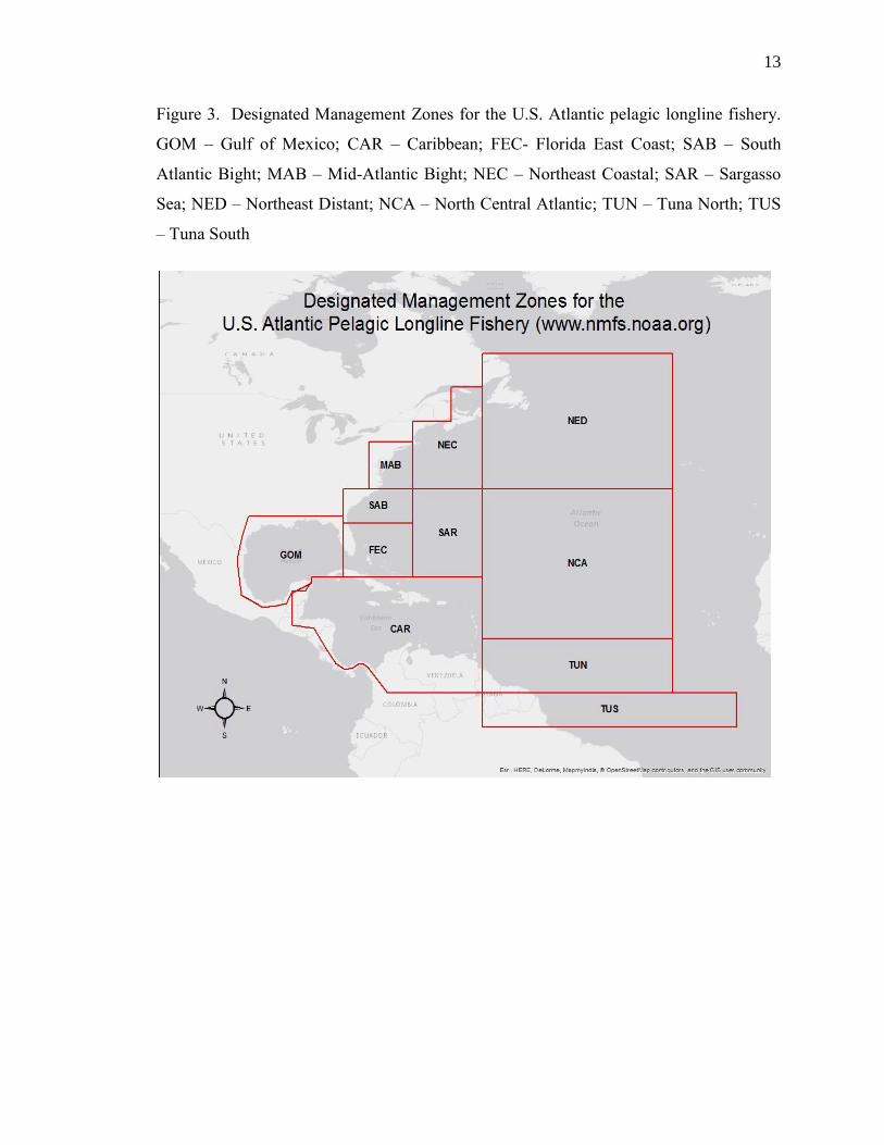
Figure 3. Designated Management Zones for the U.S. Atlantic pelagic longline fishery.

GOM – Gulf of Mexico; CAR – Caribbean; FEC- Florida East Coast; SAB – South

Atlantic Bight; MAB – Mid-Atlantic Bight; NEC – Northeast Coastal; SAR – Sargasso

Sea; NED – Northeast Distant; NCA – North Central Atlantic; TUN – Tuna North; TUS

– Tuna South

14

CPUE-based abundance indices also often assume that all non-fished areas within

a geographical range behave the same. However, CPUE data are rarely proportional to

abundance over an entire geographic region. Current and depth profiles, sea surface

temperature, depth of thermoclines, and other physical and biological parameters create

different sea conditions and influence biota differently within a large geographic area

(Maunder et al. 2006; Harley et al. 2001; Maunder and Punt 2004). Hence, CPUE should

only be used as an index of relative abundance at the spatial and temporal scales from

which it was derived. Decades of fisherman’s experience in a particular area generally

reveal well-defined areas of increased target fish catch probability within the navigable

limitations of the vessel. For the WNA PLL tuna fishery, effort is concentrated in a

relatively small part of the target species geographic range. CPUEs are extrapolated from

the fished areas to non-fished areas and are then applied to larger management areas (i.e.

the designated management zones of the U.S. PLL fishery; Fig. 3) as an index of relative

abundance. However, extrapolated abundance indices do not reflect true relative

abundance in non-fished areas due to the frequently violated assumption that individuals

are distributed proportionally throughout the species geographic range. Consequently,

stock assessments conducted for HMS from extrapolated CPUEs tend to overestimate

stock abundance (i.e., hyperstability per Harley et al. 2001)

Spatial CPUE abundance indices

The spatial distribution of fish and fishing effort is essential for understanding the

proportionality between CPUE and stock abundance (Hilborn and Walters 1987). The

distribution of HMS like tunas and swordfish are directly linked to environmental factors

that are probably the main driver in population-wide transoceanic migrations or other

movements (Maury et al. 2001). The relative movement of fisheries effort among areas

of different fish aggregations introduces biases that may lead to hyperstability or

hyperdepletion interpretations (Hilborn and Walters 1992; Carruthers et al. 2010). Figure

4 shows the changes in fishing effort and distribution for the US Atlantic tuna fleet

(Carruthers et al. 2010). The majority of misunderstanding in fisheries modeling and

management comes from dealing with these very different spatial and temporal scales

(Moustakas et al. 2006). Although the need to incorporate spatial data in CPUE-based

15

abundance indices has been well documented (Beverton and Holt 1957; Harley et al.

2001; Walters 2003; Maunder et al. 2006), abundance indices for Atlantic HMS are

continually derived without accounting for fish and fishing effort distributions

(Carruthers et al. 2010).

Several spatial analysis methods have been proposed utilizing catch and effort

data from surveys, commercial logbooks, and onboard observers. Surveys are the

preferred data source because the methods are often standardized and kept constant

through time (Maunder and Punt 2004). A study by Can et al. (2004) was able to utilize

survey data from the penaeid shrimp bottom-trawl fishery in Iskenderun Bay, Turkey, to

create a spatially-based CPUE via the “swept area” method (i.e., the effective area

covered by the trawl; commonly used for spatial CPUE based abundance indices of

bottom-trawl fisheries). In Can et al. (2004), CPUE was defined as the catch in weight

(Cw) divided by the swept area (a) for each species and for each haul:

CPUE = Cw / a (3)

Area-based methods like this are generally accepted as unbiased as long as the area is

appropriately estimated and poorly sampled areas are weighted appropriately (Sullivan

1992). Can et al. (2004) define swept area (a) with the following equation:

a = Di * h * X (4)

where Di is the covered distance, h is the head-rope length, and X is the fraction of the

head rope length that is equal to the width of the path swept by the trawl (Can et al.

2004). The distance covered (Di) was calculated by the formula,

Di = 60x √ (5)

where subscript 1 refers to latitude and longitude at the start of the haul and subscript 2

refers to latitude and longitude at the end of the haul (units were in nautical miles and

then converted to kilometers). CPUEs were computed via equation (3) for each species

16

and for each of two defined stratum. The results of this study are presented in Table 2.

In a similar study by Pezzuto et al. (2008), swept area was used to assess seabob shrimp

(Xiphopenaeus kroyeri) biomass for the artisinal shrimp trawl fishery in Southern Brazil

utilizing observer data. Because observer data are fishery-dependent and there is strong

variation between fishing effort distribution and fishing method between vessels, several

critical assumptions had to be made by Pezzuto et al. (2008) regarding catchability and

the sampling design. Inevitably, the variables used to define the effective swept-area are

generally considered on a case-by-case basis for stock abundance estimates made using

the swept-area method (Gunderson 1993).

For HMS like tunas and swordfish, data from commercial logbooks and onboard

observers are considered the only reliable data available because pelagic fisheries surveys

are generally too expensive to conduct due to the harvesting method and large-scale

migratory behavior. Pelagic fisheries surveys are also considered biased because of the

mismatch in survey locations and localized fish aggregations (ICCAT 2013). For the

WNA PLL mixed tuna and swordfish fishery (as is the case for most pelagic fisheries),

the fishery is divided into a number of regions and estimates for stock density are

obtained from logbook and onboard observer catch and effort data for each region to

account for spatial heterogeneity when deriving abundance indices (Campbell 2004).

Assuming equal catchability across all individuals and regions, average regional catch

rates weighted by size of each region gives a relatively unbiased estimate for total stock

abundance. Using this approach, Langley (2004) found that spatially-based CPUEs from

purse-seine logbooks in the west-central Pacific, although broadly similar to the nominal

CPUE, did not show any overall trend over the entire time period. Also, the magnitude

of variation in the nominal CPUE indices were far less compared to the spatially-based

indices indicating that further investigation of fishery effort distribution is warranted.

Similarly, a study by Jurado-Molina et al. (2011) developed a spatially adjusted CPUE

for the albacore fishery in the South Pacific. Based on the results, the nominal CPUE

was generally larger than the spatially adjusted CPUE and areas of high spatial CPUE

emerged within the study region. However, the resulting spatial abundance indices from

these studies are biased to favor regions with the most observations because equal weight

is given to each observation as opposed to each region (Campbell 2004).

17

Figure 4. The spatio-temporal distribution of U.S. pelagic longline effort in the western

North Atlantic. Panels represent effort in (a) 1990, (b) 1995, (c) 2000 and (d) 2005.

Effort is reported in longline hooks. Bubbles represent relative effort scaled linearly and

are comparable among panels (Carruthers et al. 2010).

18

Table 2. Spatially-based CPUE utilizing survey data from the penaeid shrimp bottom-

trawl fishery in Iskenderun Bay, Turkey. Mean CPUE (±SD) and Coefficient of

Variation (CV) for strata and total area among the species for the bottom trawl shrimp

fishery (Can et al. 2004).

Species Stratum I CV(%) Stratum II CV(%) Total Area CV(%)

P. semisulcatus 0.81 ± 0.51 63.1 12.57 ± 13.9 111.25 9.96 ± 13.29 132.8

M. stebbingi 76.38 ± 103.24 135.2 71.32 ± 60.9 85.45 73.43 ± 76.9 104.67

M. monoceros − − 47.84 ± 5.76 118.98 47.84 ± 5.80 118.98

M. japonicus 0.44 ± 0.20 45.74 1.59 ± 1.37 86.44 1.01 ± 1.10 108.78

M. kerathurus 0.47 ± 0.09 19.32 1.55 ± 1.43 92.33 1.25 ± 1.30 103.58

19

While most of the uncertainty in CPUE-based abundance indices is related to

unequal spatial distributions of target fish and effort, biases can also enter due to

inappropriate spatial scaling and missing observations (i.e., areas of fishery that are not

fished) (Campbell 2004). Not only do regions within a fishery go un-fished, but the

number and geographic location of regions fished also vary each year as a result of

fishermen’s awareness to the spatial distribution of target fish and increased ability to

find and fish those areas. This spatial contraction can occur on any scale, and all

variables should be accounted for when interpreting catch and effort data (Campbell

2004). Although GLMs are commonly used to deal with the inherent bias of nominal

CPUE for spatial analysis, they are often refuted for their inapplicable assumptions (i.e.,

catchability and spatial contraction of the fishery overtime with respect to fish

aggregations). As suggested by Campbell (2004), calculating a single reliable unbiased

relative stock abundance index without spatial analysis is generally unattainable.

Inevitably, the analysis of CPUE-based abundance indices should stem from the

understanding and concepts of spatial distribution for both fishing effort and the stock in

question. More specifically, CPUE should incorporate an area metric when used as an

abundance index within stock assessment models.

Currently, HMS fisheries use point data for spatial referencing. In 2006, for

example, NMFS implemented the Atlantic Pelagic Longline Take Reduction Plan

(PLTRP). In summation, the goal of the PLTRP was “to reduce serious injuries and

mortalities of marine mammals in the Atlantic pelagic longline fishery to insignificant

levels.” To accomplish this, the PLTRP team identified the distribution of marine

mammal interactions within the PLL fishery (Figure 5). Essentially, each point

represents the starting location of the set in which an interaction took place. Since PLL

gear frequently exceeds 30 miles in length, the point does not accurately reflect the true

location of the interaction. Additionally, the scale of spatial referencing for the WNA

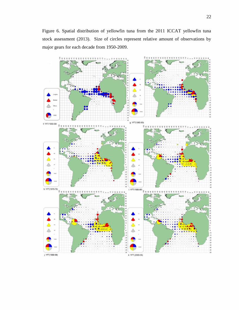
PLL fishery is extremely large. For example, Figure 6 is from the 2011 ICCAT

yellowfin tuna stock assessment to show spatial distribution of yellowfin tuna catches.

The size of the circles represent relative amount of observations that occurred within each

5 x 5 degree cell, which is a resolution on the scale of 100,000 km2. This is what is

required on an international level (ICCAT 2013), however for the U.S. PLL the spatial

20

resolution can be refined to the scale of 10-100 km2 utilizing GPS data that is currently

recorded by all NMFS observers.

The objective of this thesis is to incorporate spatial PLL data to create a spatial

CPUE (SCPUE ) for the U.S.-based PLL mixed tuna and swordfish fishery operating in

the western North Atlantic (WNA). Theoretically, the widespread use of this new metric

would increase the accuracy of abundance estimates and integrated stock assessments by

eliminating the assumption that all non-fished areas of a population’s geographic range

have the same proportion of individuals as the fished areas, and instead provide an area-

specific SCPUE. Additionally,

SCPUE may also aid fisheries managers when attempting

to identify essential fish habitat (EFH), an increasing management concern due to

legislative mandates (Magnuson-Stevens 1996). Jurado-Molina et al. (2011), among

others, eloquently explain the exponential shift in fisheries management from single-

species oriented regimes using quotas and restrictions to models that consider different

types of fishing interactions affecting other species and the ecosystem, commonly

referred to as “ecosystem-based fisheries management.” When CPUE is analyzed within

a spatial context, fisheries scientists are better able to describe particular areas of fishing

grounds in terms of fish aggregations due to the behavior of large migratory pelagic fish

species. In accordance with the same principle, spatial CPUE will identify non-target

fish aggregations and aid in the global effort to reduce bycatch and increase the

sustainability of marine fisheries. Spatial CPUE for the WNA PLL fishery will also help

identify potential areas for protection for bycatch species, such as sea turtles, marine

mammals, and sharks.

21

Figure 5. Marine mammal interactions from the 2006 Atlantic Pelagic Longline Take

Reduction Plan (2014). Each non-grey point represents the starting location of the PLL

set in which an observed marine mammal interaction occurred.

22

Figure 6. Spatial distribution of yellowfin tuna from the 2011 ICCAT yellowfin tuna

stock assessment (2013). Size of circles represent relative amount of observations by

major gears for each decade from 1950-2009.

23

Materials and Methods

Data collection

This study utilized seven years (2003-2006 and 2008-2010) of catch and effort

data from the western North Atlantic U.S. PLL fleet targeting yellowfin tuna, swordfish

and bigeye tuna. The WNA is defined herein as all waters off the U.S. east coast from

15-50º N (including the Caribbean Sea and Gulf of Mexico) extending east to the US

EEZ (Exclusive Economic Zone). The 2003 and 2004 data were collected for the

Kerstetter and Graves (2006) circle versus J-style hooks study. The 2005 and 2006 data

were obtained directly from POP electronic record logs and are the only data sets utilized

in this study lacking section-level GPS coordinates. The 2008-2010 data were collected

by trained POP observers for NSU’s time-area closure study in the FEC and SAB

management zones funded by the NMFS.

Observers were professionally trained to collect reliable catch and effort data via

standardized data sheets (Appendix I-IV). Each standardized data sheet was designed to

specifically record a particular aspect of PLL fishing operations. For example, the Gear

Log form was used to record data specific to the gear being used (e.g., type of mainline,

gangions, hooks, buoys), while the Haul Log form was used to record geographic

location information, time of fishing operations, water depth, speed, and heading, among

others. The Animal Log form was used to record each individual animal that was

observed interacting with the gear by species (i.e., all fish brought onboard, including

animals that were removed from the gear and animals that were unintentionally released,

whether alive or dead). Each data sheet included spaces for trip number, vessel name and

number, date of haul, and haul number so that all four sheets correspond and can be

traced to the same trip and set. Specific data that were utilized from each data sheet in

this study are as follows:

(1) Trip summary logs: coverage area (corresponding to the management areas in Figure

3) and number of sets observed in each coverage area. These data provided a

geographical visual of where each set occurred among the several management areas

for the WNA U.S. PLL fishery. These data sheets were available for the 2008-2010

data sets only.

24

(2) Haul Log: target species, mainline length, number of hooks set, number of sections,

and nautical coordinates at the beginning and end of both set and haul back. These

data were used to characterize the set via target species and were the basis for

calculating and developing a spatial CPUE metric. Section coordinates were also

recorded for all sets from 2003-2004 and 2008-2010 data.

(3) Gear Log: trip number, vessel name and number and date landed. These data were

used for data organization purposes.

(4) Animal Log: haul number, date of haul, the species code for each animal, and

disposition of the target species (swordfish, yellowfin and bigeye tuna) and bluefin

tuna were utilized. These data were used to create a spatial CPUE for each target

species and bycatch species, including specific species of concern.

Spatial CPUE was calculated for 22 species and species groups of the

approximately 80 different species that have historically been observed interacting with

PLL gear in the WNA (POP 2014). Three of the selected species – swordfish, yellowfin

and bigeye tuna – are primary target species of the fishery, while the remaining 19

species and species groups were specifically selected for this study because NMFS has

identified them as particular species of concern with specific objectives highlighted in the

agency’s HMS Fishery Management Plan (HMS FMP 2006). Species were also selected

due to the increasing pressure for protection from regional and federal mandates, most

notably for the highly-prized and -valued western Atlantic bluefin tuna (SAFE 2014). A

full list of species codes and species group codes used in this study are listed in Table 3.

Animals were recorded on temporary animal tally logs to expedite data entry (Appendix

V). Species that were observed on the Animal Logs, but were not listed for the purpose

of this study, were omitted from the data and were therefore not counted toward the total

animal tally.

25

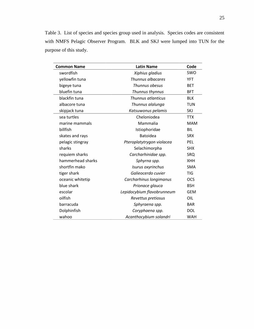
Table 3. List of species and species group used in analysis. Species codes are consistent

with NMFS Pelagic Observer Program. BLK and SKJ were lumped into TUN for the

purpose of this study.

Common Name Latin Name Code

swordfish Xiphius gladius SWO

yellowfin tuna Thunnus albacares YFT bigeye tuna Thunnus obesus BET bluefin tuna Thunnus thynnus BFT

blackfin tuna Thunnus atlanticus BLK albacore tuna Thunnus alalunga TUN

skipjack tuna Katsuwonus pelamis SKJ

sea turtles Cheloniodea TTX marine mammals Mammalia MAM billfish Istiophoridae BIL skates and rays Batoidea SRX pelagic stingray Pteroplatytrygon violacea PEL sharks Selachimorpha SHX requiem sharks Carcharhinidae spp. SRQ hammerhead sharks Sphyrna spp. XHH shortfin mako Isurus oxyrinchus SMA tiger shark Galieocerdo cuvier TIG oceanic whitetip Carcharhinus longimanus OCS

blue shark Prionace glauca BSH escolar Lepidocybium flavobrunneum GEM oilfish Revettus pretiosus OIL barracuda Sphyraena spp. BAR Dolphinfish Coryphaena spp. DOL wahoo Acanthocybium solandri WAH

26

Deriving Spatial CPUE

PLL CPUEs that are used to derive abundance indices for species in the NWA

tuna fishery are currently defined as:

CPUEspp = Nspp / 1000 hooks (6)

where Nspp is the number of fish for a species. If, for example, five yellowfin tuna (YFT)

were landed with 500 hooks deployed, then CPUEYFT = 10. Dividing equation (6) by the

total area fished by the gear during the soak gives the equation:

SCPUEspp = Nspp / 1000 hooks / An (7)

where An is the total area in km2 for set n. This equation, (7), incorporates a spatial metric

derived directly from the observed PLL set and defines the resulting spatial CPUE metric

(SCPUE) for the WNA PLL mixed tuna and swordfish fishery. As mentioned previously,

SCPUE was calculated for the target species of the fishery, as well as 19 other species or

species groups of particular concern, for each observed PLL set, and section when

applicable, within the 2003-2006 and 2008-2010 data sets.

Statistical Analysis

Non-spatial Statistical Analysis and Perceived-Area-Fished (PAF)

Standard CPUE (i.e., number of fish per 1000 hooks; the current metric for catch

per unit effort) was calculated for retained SWO for each full set (Af) from the study data

set and compared to SCPUE derived from the same data set to identify any statistical

difference between the values. Since the metrics for these values do not allow for direct

comparison (e.g., t-tests or ANOVAs), the values were compared via skewness and

kurtosis distribution analysis. For calculating the total area fished by the gear during the

soak, the nautical coordinates (i.e., latitude and longitude) recorded by the onboard

observer via handheld GPS units at the start and end of each set and haul were converted

from degrees, minutes and seconds to decimal degrees (DD). Microsoft Excel (MS Excel

27

2010) served as the data organization platform and the execution of non-spatial statistical

analysis for this study.

ESRI ArcMap 10.2 was the GIS platform used to visualize each longline set in

two-dimensions. Data was imported into ArcMap using a UTM projected coordinate

system. Polygon shapefiles (.SHP) were created by connecting the four coordinates from

the start and end of the set and haul back for both full set and section-level data, and for

all seven years. Each polygon received an individual identification number. The

resulting polygons represent the “perceived-area-fished” (PAF), or the total area that the

gear occupied as it drifted with the surface currents during the soak. The PAF in terms of

square kilometers was calculated using the calculate geometry tool in the attributes table.

The PAF provided the spatial component for SCPUE. Sections with observed part-offs

(i.e., where the mainline was severed intentionally by the fishermen or unintentionally

due to animal interaction during the haul) in excess of 30 minutes were omitted from

analysis because this scenario frequently creates uncharacteristic drift patterns. Finally,

the attributes (i.e., catch and effort data and SCPUE’s for all 22 species and species

groups) were joined to each full set and section-level polygon using the individual

identification number.

This study examined three methods of calculating PAF. The first method (Af)

using four coordinates from the start and end of the set and haulback of the full set. The

second method (As) using four coordinates for each section of longline gear. And the

third method (Afs) which uses the area of the full set via the sum of the sections that create

that same set (Figure 7). Af and Afs were compared via a two-tailed T-test (and were

similarly compared to As) to test if there was any statistical difference in PAF.

Additionally, skewness and kurtosis distribution analysis were conducted to provide

further insight about the difference between PAF values.

SCPUE’s were calculated using each PAF calculation. Since most full sets had

more than one corresponding section-level S

CPUE (i.e., SCPUE values derived using the

As PAF calculation), those values were averaged within sets creating a single section-

level SCPUE (As1) (refer to Figure 7) to allow for direct comparison of section-level

SCPUE to both full set-level

SCPUE values (i.e.,

SCPUE values derived using Af and Afs

PAF calculations) via one-way ANOVA. Pending the results of the ANOVA, SCPUE

28

values were then compared via two-tailed T-tests to identify statistical differences

between each of the three values (i.e., Af vs As1 vs Afs). SCPUE for retained SWO from

the 2009 subset was used for this analysis because it had the largest sample size with

complete section-level data (N = 66).

Hot Spot Analysis

Full set (Af) polygon .SHP files from each year (2003-2006 and 2008-2010) were

merged into a single .SHP file. Using the fishnet tool, a grid was created over the entire

study area. Each cell of the grid measured 0.1 x 0.1 DD (approximately 5 miles latitude x

6 miles longitude or 8 x 9.6 km). With the spatial join tool, the average of the attributes

falling within each cell was calculated. All of the cells in which no fishing occurred were

removed prior to analysis. The optimized “hot spot” analysis tool was used to identify

statistically significant spatial clusters of high values (hot spots) and low values (cold

spots) via the Getis-Ord Gi* statistic (ArcGIS Resources 2014). Instead of manually

selecting the appropriate scale, multiple testing, and spatial dependence criteria, the

optimized hot spot analysis tool interrogates your data and automatically determines

settings that will produce optimal hot spot analysis results. Due to the dynamic nature of

HMS, a 2 km buffer was created around each statistically significant hot spot (Figure 8A)

in order to accurately describe the hot spot in terms of area and location. New polygons

were created via a modified minimum convex polygon method (Figure 8B) using the

perimeter of the buffer as a guide. The area of the new polygon (i.e., the statistically

significant hot spot) was calculated via the same method of PAF.

The hot spot analysis method described above was applied to fishing effort

distribution, SCPUE and corresponding CPUE. Of the 22 species used in the analysis,

two were chosen as example species for results and discussion purposes: 1) retained

SWO because majority of PLL sets directly targeted SWO, and; 2) istiophorid species

(billfishes, abbreviated as BIL) because they are increasingly referenced by NMFS as

particular species of concern for management (SAFE 2014). To qualitatively explore

temporal changes in hot-spot location, the described methods were applied to the 2008-

2010 data sets which were all observed in accordance with a NOAA-funded time-area

29

closure study in the FEC and SAB statistical management zones conducted by the NSU

Fisheries Research Laboratory (Kerstetter 2011).

30

Figure 7. Three different methods for calculating perceived area fished (PAF). Inset

map: longline set #376 from 2008. The green polygon represents Af and was created

using the four coordinates from the start and end of the set and the haulback. The yellow

polygons represent As and were created using four coordinates from the start and end of

the set and haulback for each section buy. Afs is the sum of all the yellow polygons

creating the same set, and As1 is the average of all the yellow polygons from the same set.

In this example Af = 567.8 km2 and Afs = 709.2 km

2, a 25% increase in PAF. As1 is the

average of SCPUE via the As method from a set to allow for direct comparison with

SCPUEs for the full set (Af and Afs).

31

Figure 8A. ArcGIS screen shoot: 2 km buffer around cells with Gi Bin scores ≥ 2.

32

Figure 8B. ArcGIS Screen shot: minimum convex polygons created around buffer.

33

Results

Non-spatial Statistics

Data from a total of 534 PLL sets were used in this study. Approximately 40%

(n=215) of those sets had complete section-level data, with less than 30 minutes of

recovery time due to part-offs, equating to 1,403 PLL sections. These sets fished

approximately 402,711 km2 within five of 11 designated management zones for the U.S.

Atlantic PLL fishery (NEC, MAB, SAB, FEC, and GOM; Figure 9A). In total, there

were 15,686 animal interactions relevant to this study. The primary target species for

PLL sets by year are presented in Table 4. 64% of PLL sets directly targeted swordfish,

and 23% targeted both swordfish and tuna species (i.e., yellowfin and bigeye tuna; Figure

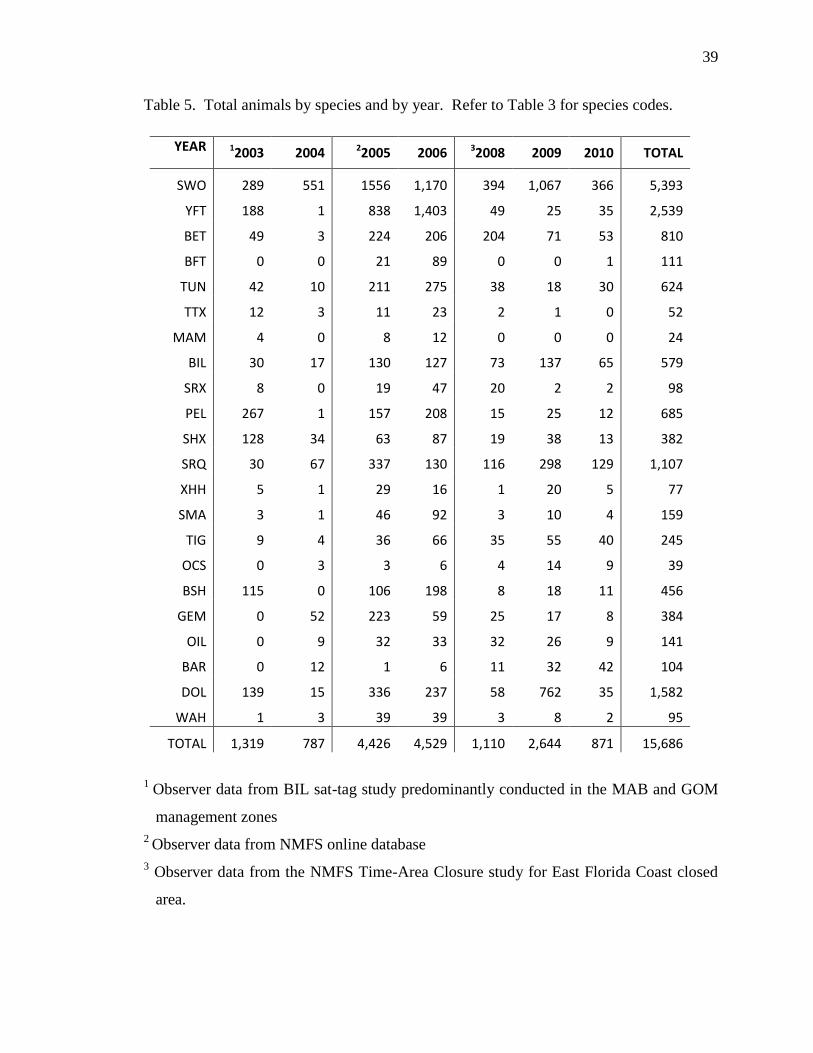
10). The number of animal interactions by species or species group code is presented in

Table 5. A complete analysis of fishing effort by year is included in Table 6.

Results of a two-tailed T-test indicate that there was no significant difference

between full set PAF calculations (Af vs Afs, p = 0.268; Table 7). As was also compared to

Af via a two-tailed T-test (p = 3.96x10-60

), although the significant difference between

these values was apparent prior to testing, since As is two to three orders of magnitude

smaller than both full set PAF calculations. Supplemental distribution analysis results

indicate that while Af and Afs are similar in distribution (K = 1.44 and 0.58; and S = 1.38

and 1.19, respectively), the distribution of As has strikingly higher skewness (S = 2.32)

and kurtosis (K = 9.32) than both Af and Afs distributions (Table 8).

The distribution analysis results of CPUE and SCPUE values indicated that both

were positively skewed (S = 2.03 and 9.32, respectively; Figure 11A and 11B); however,

the kurtosis value for SCPUE was 20 times greater compared to that of the standard

CPUE (K = 104.7 and 5.12, respectively). The range for 95% of SCPUE values is three

orders of magnitude smaller than that for CPUE (R95% = 0.17 and 47.9, respectively),

indicating much less variability in SCPUE values compared to CPUE.

Results of a one-way ANOVA (Table 9) indicate that there was a significant

difference in the means of the three SCPUE values for the 2009 subset (F = 11.96 > Fcrit,

p < 0.05). Further analysis (Table 10) indicates that SCPUE values derived from Af and

34

Afs PAF calculations did not differ significantly from each other (p > 0.05), while SCPUE

values derived from As1 differed significantly from both Af and Afs (p < 0.001).

35

Figure 9A. 2003-2006 and 2008-2010 observed pelagic longline SCPUE study sets.

Refer to Figure 3 for management zones.

36

Figure 9B. 2008-2010 observed pelagic longline SCPUE study sets.

37

Table 4. Target species for observed longline sets by year (N = 534). Refer to Table 3

for species codes.

Year SWO MIX YFT TUN DOL

2003 34 0 0 0 0

2004 38 0 0 0 0

2005 65 40 28 17 0

2006 57 73 9 11 0

2008 44 9 0 0 0

2009 68 3 0 0 4

2010 34 0 0 0 0

TOTAL 340 125 37 28 4

% Targeted 64% 23% 7% 5% 1%

38

Figure 10. Percent Species Targeted.

64%

23%

7%

5% 1%

SWO MIX YFT TUN DOL

39

Table 5. Total animals by species and by year. Refer to Table 3 for species codes.

YEAR 12003 2004 22005 2006 32008 2009 2010 TOTAL

SWO 289 551 1556 1,170 394 1,067 366 5,393

YFT 188 1 838 1,403 49 25 35 2,539

BET 49 3 224 206 204 71 53 810

BFT 0 0 21 89 0 0 1 111

TUN 42 10 211 275 38 18 30 624

TTX 12 3 11 23 2 1 0 52

MAM 4 0 8 12 0 0 0 24

BIL 30 17 130 127 73 137 65 579

SRX 8 0 19 47 20 2 2 98

PEL 267 1 157 208 15 25 12 685

SHX 128 34 63 87 19 38 13 382

SRQ 30 67 337 130 116 298 129 1,107

XHH 5 1 29 16 1 20 5 77

SMA 3 1 46 92 3 10 4 159

TIG 9 4 36 66 35 55 40 245

OCS 0 3 3 6 4 14 9 39

BSH 115 0 106 198 8 18 11 456

GEM 0 52 223 59 25 17 8 384

OIL 0 9 32 33 32 26 9 141

BAR 0 12 1 6 11 32 42 104

DOL 139 15 336 237 58 762 35 1,582

WAH 1 3 39 39 3 8 2 95

TOTAL 1,319 787 4,426 4,529 1,110 2,644 871 15,686

1 Observer data from BIL sat-tag study predominantly conducted in the MAB and GOM

management zones

2 Observer data from NMFS online database

3 Observer data from the NMFS Time-Area Closure study for East Florida Coast closed

area.

40

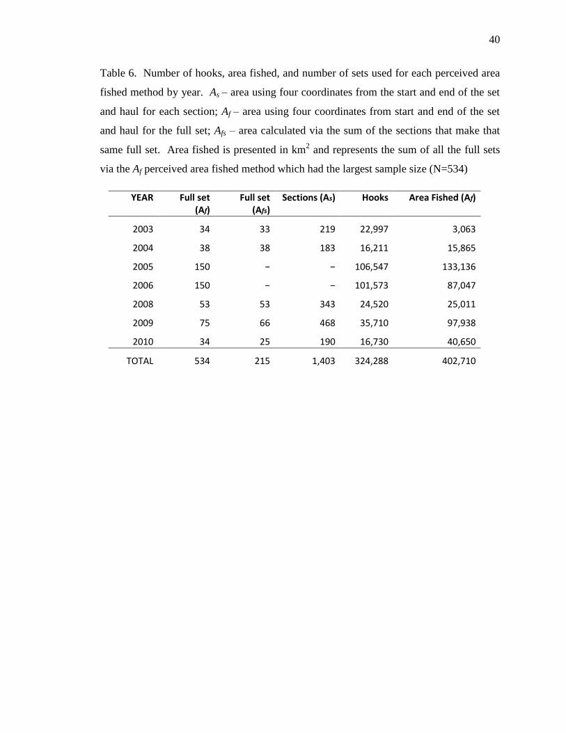
Table 6. Number of hooks, area fished, and number of sets used for each perceived area

fished method by year. As – area using four coordinates from the start and end of the set

and haul for each section; Af – area using four coordinates from start and end of the set

and haul for the full set; Afs – area calculated via the sum of the sections that make that

same full set. Area fished is presented in km2 and represents the sum of all the full sets

via the Af perceived area fished method which had the largest sample size (N=534)

YEAR Full set (Af)

Full set (Afs)

Sections (As) Hooks Area Fished (Af)

2003 34 33 219 22,997 3,063

2004 38 38 183 16,211 15,865

2005 150 − − 106,547 133,136

2006 150 − − 101,573 87,047

2008 53 53 343 24,520 25,011

2009 75 66 468 35,710 97,938

2010 34 25 190 16,730 40,650

TOTAL 534 215 1,403 324,288 402,710

41

Table 7. Perceived Area Fished (PAF) statistical analysis. As – area using four

coordinates from the start and end of the set and haul for each section; Af – area using

four coordinates from start and end of the set and haul for the full set; Afs – area

calculated via the sum of the sections that make that same full set. Results of a two-tailed

T-test (p < 0.05) indicates a statistically significant difference between the PAF

calculations. Only one full set PAF value was tested against As since the p-value from Af

and Afs is > 0.05.

Af Afs As

Mean 745.4 832.9 128.7

SD 761.1 869.2 150.2

SEM 51.9 59.3 4.0

VAR 576555.2 752067.4 22536.9

p-value (Af vs Afs) 0.267855

p-value (Af vs As) 3.96 x 10-60

42

Table 8. Perceived area fished (PAF) distribution analysis results. As – area using four

coordinates from the start and end of the set and haul for each section; Af – area using

four coordinates from start and end of the set and haul for the full set; Afs – area

calculated via the sum of the sections that make that same full set.

Area Type (km²) As Af Afs

Maximum 1,410.9 4,475.6 4,285.9 Minimum 0.10 5.44 20.50 Mean 128.7 754.1 832.9

Kurtosis 9.33 1.44 0.58 Skewness 2.32 1.38 1.19

Sample size (N) 1404 534 215

43

Figure 11A. Histogram of full set (Af) CPUE values. S – skewness; K – kurtosis; R95% –

range of 95% of values (first 5 bins); N = 534. Bin values reflect 10% increments of the

maximum CPUE value (max CPUE = 95.83 retained SWO/1000 hooks; bin range =

9.58).

17 11 4 3 2 2 0

50

100

150

200

250

300

350

1 2 3 4 5 6 7 8 9 10

nu

mb

er o

f p

elag

ic lo

ngl

ine

sets

CPUE bins

S = 2.03 K = 5.12 Mean = 12.66 R95% = 47.9

44

Figure 11B. Histogram of full set (Af) SCPUE values. S – skewness; K – kurtosis; R95% –

range of 95% of values (first bin); N= 534. Bin values reflect 10% increments of the

maximum SCPUE value (max

SCPUE = 1.74 retained SWO/1000hooks/km

2; bin range =

0.17).

18 2 1 0 1 1 0 1 1

0

100

200

300

400

500

600

1 2 3 4 5 6 7 8 9 10

nu

mb

er o

f p

elag

ic lo

ngl

ine

sets

CPUE bins

S = 9.32 K = 104.7 Mean = 0.043 R95% = 0.17

45

Table 9. Summary and results of one-way ANOVA for three methods of calculating

SCPUE for retained SWO via different PAF calculations for the 2009 subset. As – area

using four coordinates from the start and end of the set and haul for each section; Af –

area using four coordinates from start and end of the set and haul for the full set; Afs –

area calculated via the sum of the sections that make that same full set; As1 is the average

of As for the full set. F > Fcrit and p-value < 0.05, therefore a statistically significant

difference exists between the three values.

SCPUE methods Count Sum Average Variance

Af 66 − 0.0305 0.0018

Afs 66 − 0.0300 0.0022

As1 66 − 0.3334 0.5035

Source of Variation SS df MS F P-value F crit

Between Groups 4.04 2 2.02 11.96 1.26x10-5 3.04 Within Groups 32.98 195 0.17

Total 37.03 197

46

Table 10. Results of two-tailed T-test for three methods of calculating SCPUE for

retained SWO via different PAF calculations for the 2009 subset. As – area using four

coordinates from the start and end of the set and haul for each section; Af – area using

four coordinates from start and end of the set and haul for the full set; Afs – area

calculated via the sum of the sections that make that same full set; As1 is the average of As

for the full set. As1 is statistically different from both Af and Afs (p-value < 0.001).

Af Afs As1

MEAN 0.0305 0.0300 0.3334

SD 0.0418 0.0472 0.7096

SEM 0.0051 0.0058 0.0873

VAR 0.0017 0.0022 0.4959

p-value (Af vs Afs) 0.946331

p-value (Af vs As1) 0.000725

p-value (As1 vs Afs) 0.000935

47

Spatial Statistics

The optimized hot spot analysis identified statistically significant hot spots and

cold spots for fishing effort distribution and for SCPUE and CPUE for both retained

SWO and BIL. However, since this thesis focuses on areas of concentrated PLL fishing

effort and areas of relatively higher SCPUE and CPUE values, only hot spot results (i.e.,

grid cells with Gi_BIN scores ≥ 2 = 95% confidence) will be presented and discussed.

Using the merged .SHP file of all full set (Af) polygons, five statistically

significant fishing effort distribution hot spots were identified (Figure 12). The two

largest were in the SAB and FEC management zones (22,756 and 16,167 km2,

respectively). Two hot spots were identified in the GOM (7,445 and 3,651 km2), and one

hot spot identified in the MAB (3,432 km2). No hot spots were identified in the NEC

management zone. There were 12 hot spots identified for SCPUE values of retained

SWO (Figure 13A), while only eight hotspots were identified for corresponding CPUE

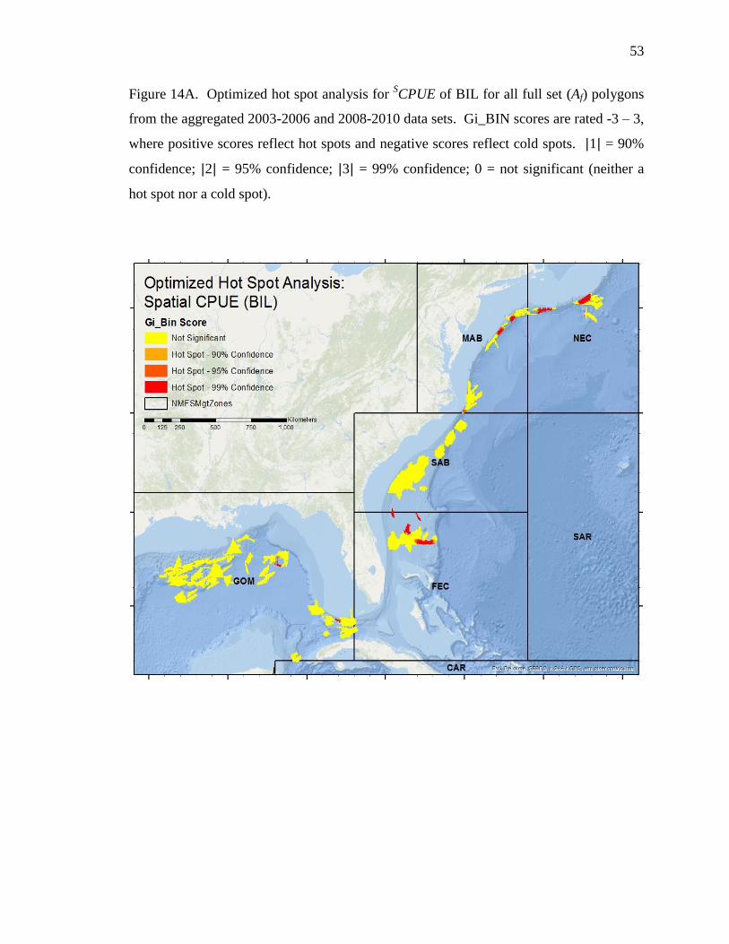
values (Figure 13B). Adversely, 11 hot spots were identified for SCPUE values of BIL

(Figure 14A), while 19 hot spots were identified for corresponding CPUE values (Figure

14B). Hot spot areas (km2) for fishing effort distribution,

SCPUE and CPUE for both

BIL and retained SWO by management zone are presented in Table 11.

Using the merged .SHP file for the 2008-2010 subset of full set (Af) polygons in

the SAB and FEC, two statistically significant fishing effort distribution hot spots were

identified in the SAB and FEC (1,748 and 8,965 km2, respectively). Additionally, one

hot spot of fishing effort was identified within each year. Statistically significant hot

spots were identified for SCPUE and CPUE, for both retained SWO and BIL, collectively

and within years 2008-2010. The spatio-temporal relationship between hot spots is

thoroughly discussed in the following section. Hot spot areas (km2) for fishing effort

distribution, SCPUE and CPUE of both BIL and retained SWO for the 2008-2010 subsets

are presented in Table 12. All figures for temporal analysis results are referenced in the

temporal analysis discussion section.

48

Table 11. Hot spot areas (km2) for fishing effort distribution,

SCPUE and CPUE for both

BIL and retained SWO by management zone. GOM – Gulf of Mexico; FEC – Florida

East Coast; SAB – South Atlantic Bight; MAB – Mid-Atlantic Bight; NEC – Northeast

Coastal. Outliers highlighted in red are only associated with one observed PLL set in that

location and are not included in the discussion section.

Management Zone

Hotspot Number

Effort CPUE SCPUE

SWO BIL SWO BIL

GOM 1 3,651.12 3,760.65 1,009.06 2,535.53 2,454.56 2 7,445.31 5,480.96 2,247.10 4,429.33 898.23 3 - 15,262.82 2,113.21 1,196.86 - 4 - - 374.37 - - 5 - - 5,221.60 - - 6 - - 2,610.07 - - 7 - - 1,648.33 - - 8 - - 337.40 - -

FEC 1 16,167.59 6,379.23 31,965.46 928.44 3,986.47 2 - - 989.40 - 2,601.78 3 - - 989.30 - 977.65 4 - - - 1,001.77

SAB 1 22,756.89 31,247.88 3,254.40 1,670.48 557.35 2 - - 1,045.19 2,857.30 - 3 - - 3,067.46 - - 4 - - 3,981.36 - -

MAB 1 3,432.91 2,324.06 1,021.33 562.81 1,209.62 2 - 862.66 677.61 1,082.52 1,009.23 3 - - 733.11 1,032.15 - 4 - - - 784.52 -

NEC 1 - 443.42 1,888.30 1,247.80 2,162.53 2 - - - 2,120.97 2,707.01

49

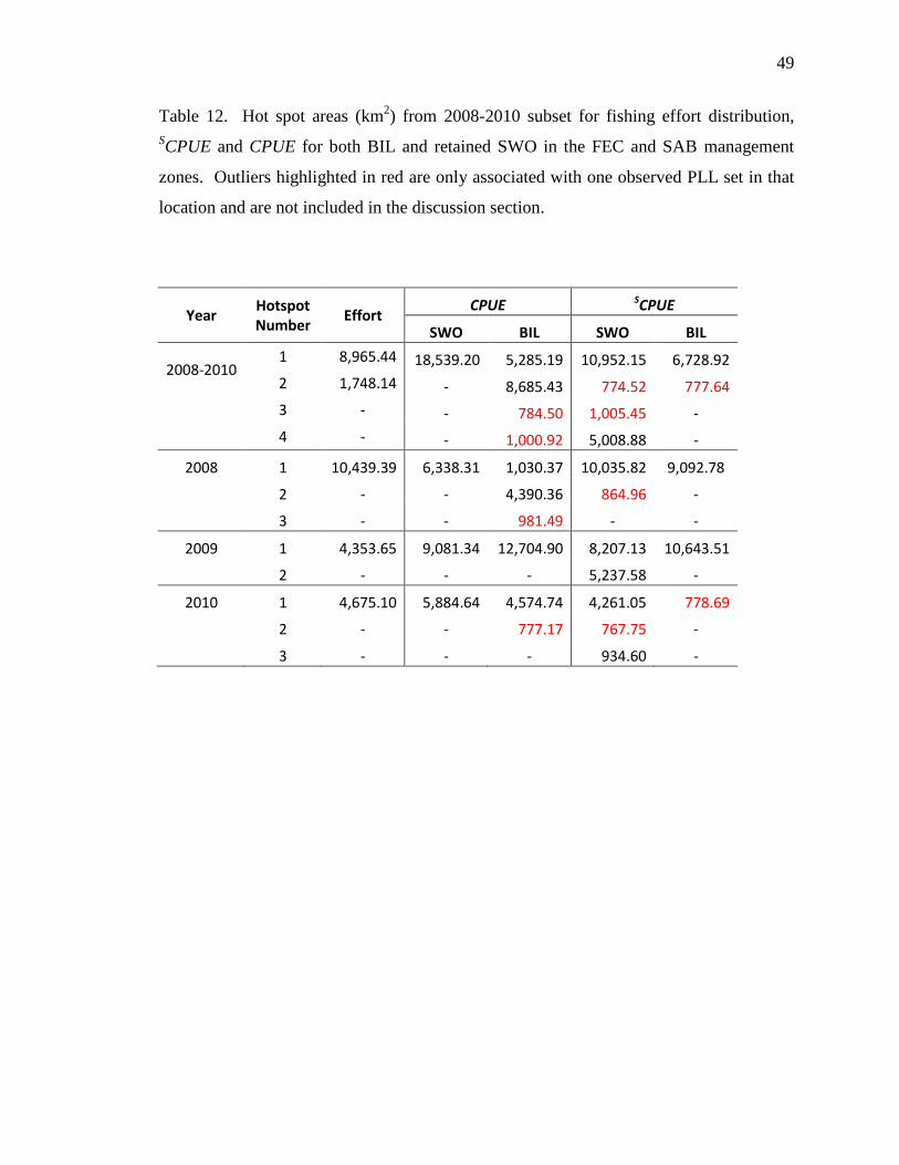
Table 12. Hot spot areas (km2) from 2008-2010 subset for fishing effort distribution,

SCPUE and CPUE for both BIL and retained SWO in the FEC and SAB management

zones. Outliers highlighted in red are only associated with one observed PLL set in that

location and are not included in the discussion section.

Year Hotspot Number

Effort CPUE SCPUE

SWO BIL SWO BIL

2008-2010 1 8,965.44 18,539.20 5,285.19 10,952.15 6,728.92

2 1,748.14 - 8,685.43 774.52 777.64

3 - - 784.50 1,005.45 -

4 - - 1,000.92 5,008.88 -

2008 1 10,439.39 6,338.31 1,030.37 10,035.82 9,092.78

2 - - 4,390.36 864.96 -

3 - - 981.49 - -

2009 1 4,353.65 9,081.34 12,704.90 8,207.13 10,643.51

2 - - - 5,237.58 -

2010 1 4,675.10 5,884.64 4,574.74 4,261.05 778.69

2 - - 777.17 767.75 -

3 - - - 934.60 -

50

Figure 12. Optimized hot spot analysis for fishing effort distribution of all full set (Af)

polygons from the aggregated 2003-2006 and 2008-2010 data sets. Gi_BIN scores are

rated -3 – 3, where positive scores reflect hot spots and negative scores reflect cold spots.

1 = 90% confidence; 2 = 95% confidence; 3 = 99% confidence; 0 = not significant

(neither a hot spot nor a cold spot).

51

Figure 13A. Optimized hot spot analysis for SCPUE of retained SWO for all full set (Af)

polygons from the aggregated 2003-2006 and 2008-2010 data sets. Gi_BIN scores are

rated -3 – 3, where positive scores reflect hot spots and negative scores reflect cold spots.

1 = 90% confidence; 2 = 95% confidence; 3 = 99% confidence; 0 = not significant

(neither a hot spot nor a cold spot).

52

Figure 13B. Optimized hot spot analysis for CPUE of retained SWO for all full set (Af)

polygons from the aggregated 2003-2006 and 2008-2010 data sets. Gi_BIN scores are

rated -3 – 3, where positive scores reflect hot spots and negative scores reflect cold spots.

1 = 90% confidence; 2 = 95% confidence; 3 = 99% confidence; 0 = not significant

(neither a hot spot nor a cold spot).

53

Figure 14A. Optimized hot spot analysis for SCPUE of BIL for all full set (Af) polygons

from the aggregated 2003-2006 and 2008-2010 data sets. Gi_BIN scores are rated -3 – 3,

where positive scores reflect hot spots and negative scores reflect cold spots. 1 = 90%

confidence; 2 = 95% confidence; 3 = 99% confidence; 0 = not significant (neither a

hot spot nor a cold spot).

54

Figure 14B. Optimized hot spot analysis for CPUE of BIL for all full set (Af) polygons

from the aggregated 2003-2006 and 2008-2010 data sets. Gi_BIN scores are rated -3 – 3,

where positive scores reflect hot spots and negative scores reflect cold spots. 1 = 90%

confidence; 2 = 95% confidence; 3 = 99% confidence; 0 = not significant (neither a

hot spot nor a cold spot).

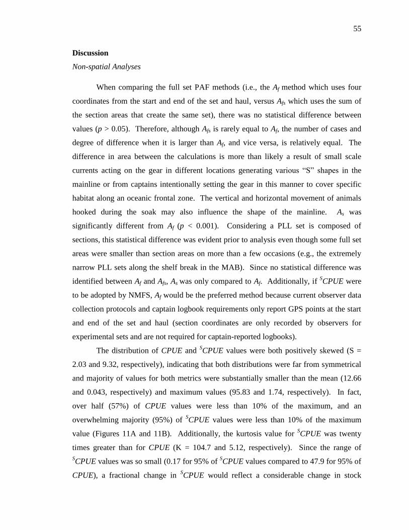
55

Discussion

Non-spatial Analyses

When comparing the full set PAF methods (i.e., the Af method which uses four

coordinates from the start and end of the set and haul, versus Afs which uses the sum of

the section areas that create the same set), there was no statistical difference between

values (p > 0.05). Therefore, although Afs is rarely equal to Af, the number of cases and

degree of difference when it is larger than Af, and vice versa, is relatively equal. The

difference in area between the calculations is more than likely a result of small scale

currents acting on the gear in different locations generating various “S” shapes in the

mainline or from captains intentionally setting the gear in this manner to cover specific

habitat along an oceanic frontal zone. The vertical and horizontal movement of animals

hooked during the soak may also influence the shape of the mainline. As was

significantly different from Af (p < 0.001). Considering a PLL set is composed of

sections, this statistical difference was evident prior to analysis even though some full set

areas were smaller than section areas on more than a few occasions (e.g., the extremely

narrow PLL sets along the shelf break in the MAB). Since no statistical difference was

identified between Af and Afs, As was only compared to Af. Additionally, if SCPUE were

to be adopted by NMFS, Af would be the preferred method because current observer data

collection protocols and captain logbook requirements only report GPS points at the start

and end of the set and haul (section coordinates are only recorded by observers for

experimental sets and are not required for captain-reported logbooks).

The distribution of CPUE and SCPUE values were both positively skewed (S =

2.03 and 9.32, respectively), indicating that both distributions were far from symmetrical

and majority of values for both metrics were substantially smaller than the mean (12.66

and 0.043, respectively) and maximum values (95.83 and 1.74, respectively). In fact,

over half (57%) of CPUE values were less than 10% of the maximum, and an

overwhelming majority (95%) of SCPUE values were less than 10% of the maximum

value (Figures 11A and 11B). Additionally, the kurtosis value for SCPUE was twenty

times greater than for CPUE (K = 104.7 and 5.12, respectively). Since the range of

SCPUE values was so small (0.17 for 95% of

SCPUE values compared to 47.9 for 95% of

CPUE), a fractional change in SCPUE would reflect a considerable change in stock

56

abundance if used as an index of relative abundance. Whereas, when CPUE is used as an

index of relative abundance, a change in stock abundance would be less noticeable. This

supports the theory that SCPUE is more accurate than CPUE when used as an index of

relative abundance by utilizing spatial information obtained directly from the fishing

location (Hilborn and Walters 1987 and 1992; Harley et al. 2001; Campbell 2004;

Maunder et al. 2006).

Statistical differences existed between the means of SCPUE using the three

different PAF calculations (Af vs. Afs vs. As1; F = 11.96 > Fcrit). Further analysis revealed

that SCPUE derived via the As method was statistically different from both Af and Afs (p <

0.001) which was consistent with the T-test comparing PAF calculations. Although the

number of hooks deployed in each section was proportional to the whole set, the area of

each section is highly variable (most likely due to small-scale current effects) and often

disproportionally smaller compared to the area of the full set (Table 10). Additionally,

the number of animals hooked in each section is not consistent throughout the set.

Typically the bulk of animals hooked on any given PLL set come from one or a few

sections. This phenomenon stems from the ecology of HMS, many of which exhibit

schooling behavior in a large-scale habitat (e.g., tuna species), and the design of PLL gear

which effectively targets HMS, among other reasons, by deploying a very long mainline

thus increasing the probability of transecting a school of target fish. Assuming

standardized deployment (i.e., that buoy configuration, leader length, bait and hook type

were the same throughout), the expectation of catching target fish in general is justifiable;

however, the expectation to catch target fish in a particular location along the 30 nautical

mile-long mainline is questionable. Inevitably, the high variability of SCPUE between

neighboring sections, coupled with the migratory behavior of HMS, creates additional

uncertainty when interpreting section-level SCPUE as an index for relative abundance.

Optimized Hot Spot Spatial Analysis

Optimized hot spot analyses were conducted to identify areas of high values that

were statistically different from a randomized distribution (i.e., areas with Gi_BIN Scores

≥ 2, corresponding to 95% confidence that a hot spot is a “true” hot spot). Full set

polygons created via the Af method were used for analysis since no statistical difference

57

between Af and Afs methods were identified and both were less variable than the As

method. Furthermore, the Af method is more applicable to management due to current

observer protocols and captain logbook reporting requirements. For CPUE and SCPUE,

hot spots represent areas of relatively high values compared to neighboring areas and are

interpreted as areas where fish tend to aggregate within the area of observed fishing

effort. For fishing effort distribution, hot spots represent areas of concentrated fishing

effort in terms of relatively high numbers of observed PLL sets compared to neighboring

areas and also provide insight into captain behavior towards fishing location. Five

statistically significant hot spots of concentrated fishing effort were identified. Refer to

Figure 12 for all references to fishing effort distribution hot spots. CPUE and SCPUE are

expressed using the species three-letter code (plus a letter representing disposition when

applicable) as a subscript to the referenced catch rate (e.g., SCPUESWOr is spatial catch per

unit effort for retained swordfish; CPUEBIL is catch per unit effort for Istiophorid species)

South Atlantic Bight (SAB)

The largest fishing effort hot spot was within the South Atlantic Bight (SAB)

(22,757 km2) and extended northward along the 200 m (700 ft) isobath from Jekyll

Island, Georgia, to approximately 100 km (62 mi) southeast of Long Bay, South

Carolina. The hot spot extended eastward over the northern edge of the Blake Plateau

approximately 110 km (68 mi) to a maximum depth of roughly 915 m (3000 ft). The

fishing effort hot spot lies completely within the hot spot that was identified for

CPUESWOr (31,248 km2). In fact, the hot spot for CPUESWOr extends an additional 100

km east-northeast along the 200 m isobath (Figure 15). Adversely, the hot spots for

SCPUESWOr (Figure 16) are much smaller (1,670 and 2,857 km

2, respectively) and are

located almost completely outside the northward boundary of the fishing effort hot spot.

Essentially, these explicitly smaller hot spots identify target SWO [i.e., LJFL ≥ 47 in (119

cm), or CK ≥ 25 in (63 cm);

Lower Jaw Fork Length (LJFL) – a straight line

measurement from the tip of the lower jaw to the fork of the caudal fin; Cleithrum to

Caudal Keel – a curved measurement from the cleithrum to the anterior portion of the

caudal keel (HMS Commercial Compliance Guide 2014)] aggregations within the

distribution of fishing effort. In theory, if vessels concentrated fishing effort in these

58

Figure 15. CPUESWOr optimized hot spot analysis in the South Atlantic Bight (SAB) and

Florida East Coast (FEC) management zones. Gi_BIN scores are rated -3 – 3, where

positive scores reflect hot spots and negative scores reflect cold spots. 1 = 90%

confidence; 2 = 95% confidence; 3 = 99% confidence; 0 = not significant (neither a

hot spot nor a cold spot). Solid black line delineates boundary between SAB and FEC.

59

Figure 16. SCPUESWOr optimized hot spot analysis in the South Atlantic Bight (SAB) and

Florida East Coast (FEC) management zones. Gi_BIN scores are rated -3 – 3, where

positive scores reflect hot spots and negative scores reflect cold spots. 1 = 90%

confidence; 2 = 95% confidence; 3 = 99% confidence; 0 = not significant (neither a

hot spot nor a cold spot). Solid black line delineates boundary between SAB and FEC.

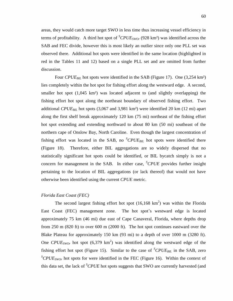
60

areas, they would catch more target SWO in less time thus increasing vessel efficiency in

terms of profitability. A third hot spot of SCPUESWOr (928 km²) was identified across the

SAB and FEC divide, however this is most likely an outlier since only one PLL set was

observed there. Additional hot spots were identified in the same location (highlighted in

red in the Tables 11 and 12) based on a single PLL set and are omitted from further

discussion.

Four CPUEBIL hot spots were identified in the SAB (Figure 17). One (3,254 km²)

lies completely within the hot spot for fishing effort along the westward edge. A second,

smaller hot spot (1,045 km²) was located adjacent to (and slightly overlapping) the

fishing effort hot spot along the northeast boundary of observed fishing effort. Two

additional CPUEBIL hot spots (3,067 and 3,981 km²) were identified 20 km (12 mi) apart

along the first shelf break approximately 120 km (75 mi) northeast of the fishing effort

hot spot extending and extending northward to about 80 km (50 mi) southeast of the

northern cape of Onslow Bay, North Caroline. Even though the largest concentration of

fishing effort was located in the SAB, no SCPUEBIL hot spots were identified there

(Figure 18). Therefore, either BIL aggregations are so widely dispersed that no

statistically significant hot spots could be identified, or BIL bycatch simply is not a

concern for management in the SAB. In either case, SCPUE provides further insight

pertaining to the location of BIL aggregations (or lack thereof) that would not have

otherwise been identified using the current CPUE metric.

Florida East Coast (FEC)

The second largest fishing effort hot spot (16,168 km2) was within the Florida

East Coast (FEC) management zone. The hot spot’s westward edge is located

approximately 75 km (46 mi) due east of Cape Canaveral, Florida, where depths drop

from 250 m (820 ft) to over 600 m (2000 ft). The hot spot continues eastward over the

Blake Plateau for approximately 150 km (93 mi) to a depth of over 1000 m (3280 ft).

One CPUESWOr hot spot (6,379 km2) was identified along the westward edge of the

fishing effort hot spot (Figure 15). Similar to the case of SCPUEBIL in the SAB, zero

SCPUESWOr hot spots for were identified in the FEC (Figure 16). Within the context of

this data set, the lack of SCPUE hot spots suggests that SWO are currently harvested (and

61

BIL are currently avoided) in the most economically sustainable way possible with PLL

gear in this geographic region.

One very large CPUEBIL hot spot (31,965 km2; Figure 17) was identified in the

FEC and completely encompasses all of the observed fishing effort, and two S

CPUEBIL

hot spots (Figure 18) were identified within that hot spot along the northward (3,986 km2)

and southeastward (2,602 km2) boundaries. Vessels may wish to avoid operating in those

particular areas due to increased BIL aggregations. Concentrating fishing efforts outside

of these areas would decrease BIL interactions thus providing the greatest opportunity to

catch target fish (i.e., fewer hooks and/or bait consumed by billfish). Fortunately, these

two hot spots are located outside the area of concentrated fishing effort, suggesting that

PLL vessels are already actively minimizing BIL interactions in this geographic region

assuming observer presence does not effect vessel fishing location.

62

Figure 17. CPUEBIL optimized hot spot analysis in the South Atlantic Bight (SAB) and

Florida East Coast (FEC) management zones. Gi_BIN scores are rated -3 – 3, where

positive scores reflect hot spots and negative scores reflect cold spots. 1 = 90%

confidence; 2 = 95% confidence; 3 = 99% confidence; 0 = not significant (neither a

hot spot nor a cold spot). Solid black line delineates boundary between SAB and FEC.

63

Figure 18. SCPUEBIL optimized hot spot analysis in the South Atlantic Bight (SAB) and

Florida East Coast (FEC) management zones. Gi_BIN scores are rated -3 – 3, where

positive scores reflect hot spots and negative scores reflect cold spots. 1 = 90%

confidence; 2 = 95% confidence; 3 = 99% confidence; 0 = not significant (neither a

hot spot nor a cold spot). Solid black line delineates boundary between SAB and FEC.

64

Gulf of Mexico (GOM)

Two much smaller fishing effort hot spots were identified in the Gulf of Mexico

(GOM). Although PLL effort was the most widely distributed visually in the GOM

compared to other management zones, the two hot spots were identified only 100 km (46

mi) apart. It is important to note, however, that most PLL effort in the northern Gulf of

Mexico was targeting YFT, which employs slightly different techniques (e.g., bait type,

space between gangions, fishing depth) compared to targeting SWO. The larger of the

two hot spots (7,445 km2) was located just south of the Dry Tortugas extending

southward from the shelf break to the Mitchell Escarpment at an approximate depth of

1,100 m (3,600 ft). The smaller hot spot (3,651 km2) was located roughly 100 km (46

mi) west of the Dry Tortugas and is situated over a series of canyons, including the

Florida Canyon, at the southern edge of the West Florida Escarpment.

Two CPUESWOr hot spots were identified in the GOM (Figure 19). The first

(5,481 km2) overlaps the eastward side of the northern fishing effort hot spot, extending

north and south an additional 10-20 km (6-12 mi) along the shelf break. The second

CPUESWOr hot spot (15,263 km2) completely encompasses the southern fishing effort hot

spot and extends into deeper waters some 20 km (12 mi) north of Havana, Cuba, and

continuing eastward over the GOM/FEC management zone divide. A third CPUESWOr hot

spot (3,761 km2) was identified approximately 100 km (46 mi) west of the Gulfo de

Guanahacabibes, Cuba, and is situated over the southern edge of the Tulum Terrace at

approximately 1000 m (3280 ft) depth. Concurrently, three SCPUESWOr were identified in

the same locations (Figure 20). The hot spot coinciding with the series of canyons at the

southern edge of the West Florida Escarpment is roughly the same area (4,429 km2) and

location as the CPUESWOr hot spot. This probably is not coincidental, and more likely a

result of experienced captains who have targeted SWO in these waters for many years

and continue to pass that knowledge to current and future generations of PLL fishermen.

The hot spot coinciding with the area over the Tulum Terrace is smaller (2,536 km2) than

the hot spot for CPUESWOr and overlaps the southern portion, implying that the southern

portion may warrant additional monitoring due to aggregations of target SWO. The last,

and smallest, SCPUESWOr hot spot (1,197 km

2) in the GOM is situated directly over the

Tortugas Terrace and Valley at the northwest corner of the CPUESWOr and fishing effort

65

hot spots. This hot spot is significantly smaller than other hot spots in the region

indicating that fishermen may wish to concentrate their efforts here in order to take

advantage of the small-scale area where target SWO aggregate.

Three CPUEBIL hot spots were identified in the GOM (Figure 21) that correlate

with fishing effort hot spots and an additional five were identified in the northern GOM,

south of the shelf edge, scattered across the ridges, valleys and escarpments of the

continental slope. However, only two SCPUEBIL hot spots were identified here (Figure

22). The smaller of the two is situated over the Tortugas Terrace and Valley, similar to

the SCPUESWOr hot spot mentioned above. The larger

SCPUEBIL hot spot (2,455 km

2),

and the largest CPUEBIL hot spot (5,222 km2), is located near the De Soto Canyon, an

area which was closed off to PLL gear in November of 2000 in order to reduce incidental

catch of undersized SWO (SAFE 2014). Since this area is historically identified for

undersized SWO, it makes sense that it is not a hot spot for retained SWO, but is still

frequented by PLL vessels due to occasional legal-sized individuals. Nevertheless,

SCPUEBIL identifies two particular areas of concern in terms of BIL bycatch that would

not otherwise be identified with current CPUE spatial-referencing methods.

66

Figure 19. CPUESWOr optimized hot spot analysis in the Gulf of Mexico (GOM)

management zones. Gi_BIN scores are rated -3 – 3, where positive scores reflect hot

spots and negative scores reflect cold spots. 1 = 90% confidence; 2 = 95%

confidence; 3 = 99% confidence; 0 = not significant (neither a hot spot nor a cold spot).

Solid black line delineates boundary between management zones.

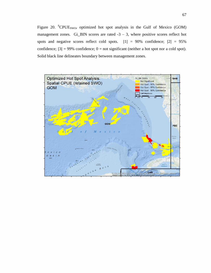
67

Figure 20. SCPUESWOr optimized hot spot analysis in the Gulf of Mexico (GOM)

management zones. Gi_BIN scores are rated -3 – 3, where positive scores reflect hot

spots and negative scores reflect cold spots. 1 = 90% confidence; 2 = 95%

confidence; 3 = 99% confidence; 0 = not significant (neither a hot spot nor a cold spot).

Solid black line delineates boundary between management zones.

68

Figure 21. CPUEBIL optimized hot spot analysis in the Gulf of Mexico (GOM)

management zones. Gi_BIN scores are rated -3 – 3, where positive scores reflect hot

spots and negative scores reflect cold spots. 1 = 90% confidence; 2 = 95%

confidence; 3 = 99% confidence; 0 = not significant (neither a hot spot nor a cold spot).

Solid black line delineates boundary between management zones.

69

Figure 22. SCPUEBIL optimized hot spot analysis in the Gulf of Mexico (GOM)

management zones. Gi_BIN scores are rated -3 – 3, where positive scores reflect hot

spots and negative scores reflect cold spots. 1 = 90% confidence; 2 = 95%

confidence; 3 = 99% confidence; 0 = not significant (neither a hot spot nor a cold spot).

Solid black line delineates boundary between management zones.

70

Mid-Atlantic Bight (MAB) and Northeast Coastal (NEC)

The smallest fishing effort hot spot was identified in the Mid-Atlantic Bight

(MAB) (3,433 km2) situated over a series of canyons approximately 60 km (37) east-

northeast of Pamlico Sound. No fishing effort hot spots were identified in the Northeast

Coastal (NEC) management zone. Unlike within other management zones, where CPUE

and SCPUE hot spots were generally in close proximity to a fishing effort hot spot, there

was very little association with fishing effort hot spots in the MAB and NEC. One

CPUEBIL (Figure 23) and one S

CPUEBIL (Figure 24) hot spot was identified in association

with the fishing effort hot spot (both were situated just south of the hot spot along the

shelf break). The rest of the hot spots generally coincided with each other and were

sporadically spaced along the shelf break east of New Jersey and south of the Georges

Bank. There were three CPUESWOr (Figure 25) hot spots identified. Two were identified

in association with the fishing effort hot spot; one situated just north (863 km2) and the

other just east (2,324 km2). The third hot spot (443 km

2) is located near the

northwestward edge of observed fishing effort in the NEC. Six SCPUESWOr hot spots

(Figure 26) were identified in the MAB and NEC. Only one is situated in close

proximity to the fishing effort hot spot while the other five are sporadically spaced along

the shelf break similar to both BIL hot spots.

Fishing effort in the MAB and NEC was observed over a series of canyons cutting

diagonally through the management zones along the shelf break. The PAF of PLL sets in

this region were characteristically narrower compared to other regions and seemingly

strategically set to minimize east-west drift and maximize fishing time over the canyons

during the soak. According to the location of SCPUE hot spots, it was inferred that BIL

and target SWO aggregate in and around specific canyons based on habitat suitability

requirements (e.g., bathymetry, surface and bottom currents, prey availability). Vessels

could increase catch of target SWO by concentrating fishing efforts near canyons

associated with SCPUE hot spots.

71

Figure 23. CPUESWOr optimized hot spot analysis in the Mid-Atlantic Bight (MAB) and

Northeast Coastal (NEC) management zones. Gi_BIN scores are rated -3 – 3, where

positive scores reflect hot spots and negative scores reflect cold spots. 1 = 90%

confidence; 2 = 95% confidence; 3 = 99% confidence; 0 = not significant (neither a

hot spot nor a cold spot). Solid black line delineates boundary between management

zones.

72

Figure 24. SCPUESWOr optimized hot spot analysis in the Mid-Atlantic Bight (MAB) and

Northeast Coastal (NEC) management zones. Gi_BIN scores are rated -3 – 3, where

positive scores reflect hot spots and negative scores reflect cold spots. 1 = 90%

confidence; 2 = 95% confidence; 3 = 99% confidence; 0 = not significant (neither a

hot spot nor a cold spot). Solid black line delineates boundary between management

zones.

73

Figure 25. CPUEBIL optimized hot spot analysis in the Mid-Atlantic Bight (MAB) and

Northeast Coastal (NEC) management zones. Gi_BIN scores are rated -3 – 3, where

positive scores reflect hot spots and negative scores reflect cold spots. 1 = 90%

confidence; 2 = 95% confidence; 3 = 99% confidence; 0 = not significant (neither a

hot spot nor a cold spot). Solid black line delineates boundary between management

zones.

74

Figure 26. SCPUEBIL optimized hot spot analysis in the Mid-Atlantic Bight (MAB) and

Northeast Coastal (NEC) management zones. Gi_BIN scores are rated -3 – 3, where

positive scores reflect hot spots and negative scores reflect cold spots. 1 = 90%

confidence; 2 = 95% confidence; 3 = 99% confidence; 0 = not significant (neither a

hot spot nor a cold spot). Solid black line delineates boundary between management

zones.

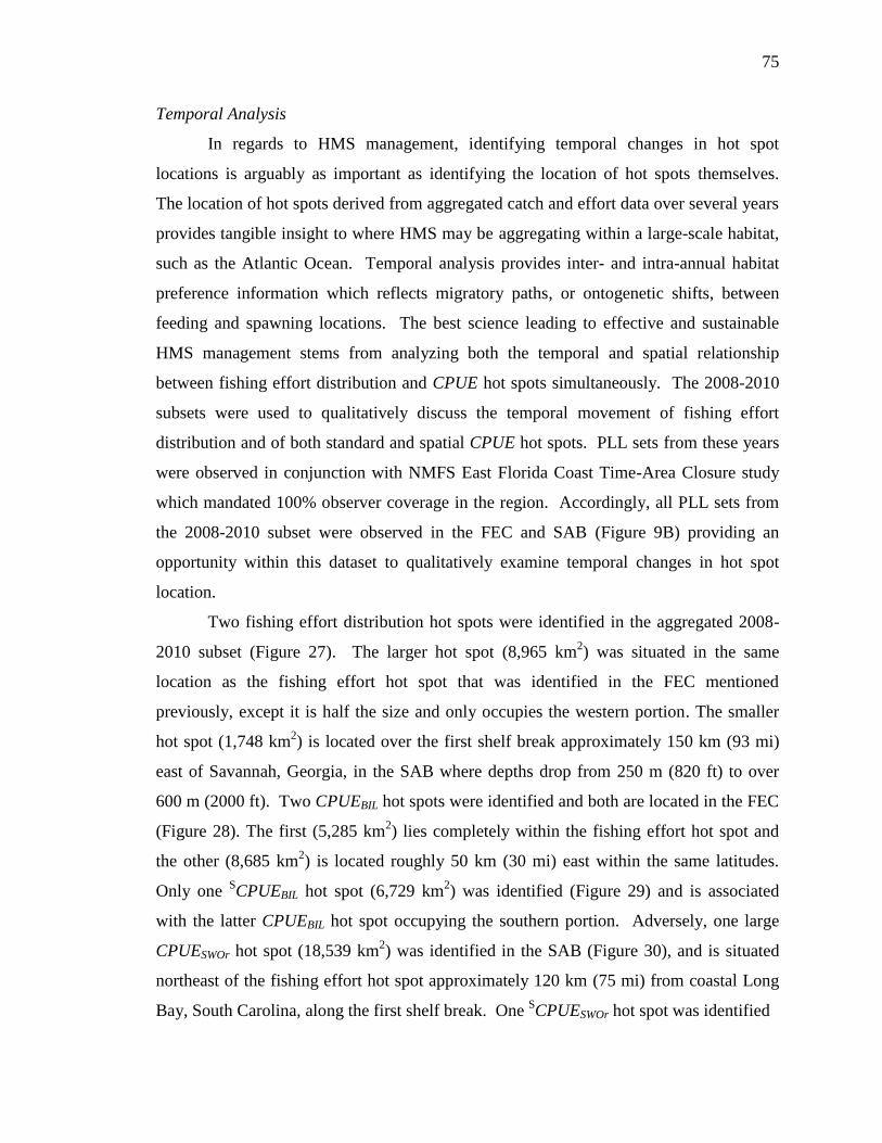
75

Temporal Analysis

In regards to HMS management, identifying temporal changes in hot spot

locations is arguably as important as identifying the location of hot spots themselves.

The location of hot spots derived from aggregated catch and effort data over several years

provides tangible insight to where HMS may be aggregating within a large-scale habitat,

such as the Atlantic Ocean. Temporal analysis provides inter- and intra-annual habitat

preference information which reflects migratory paths, or ontogenetic shifts, between

feeding and spawning locations. The best science leading to effective and sustainable

HMS management stems from analyzing both the temporal and spatial relationship

between fishing effort distribution and CPUE hot spots simultaneously. The 2008-2010

subsets were used to qualitatively discuss the temporal movement of fishing effort

distribution and of both standard and spatial CPUE hot spots. PLL sets from these years

were observed in conjunction with NMFS East Florida Coast Time-Area Closure study

which mandated 100% observer coverage in the region. Accordingly, all PLL sets from

the 2008-2010 subset were observed in the FEC and SAB (Figure 9B) providing an

opportunity within this dataset to qualitatively examine temporal changes in hot spot

location.

Two fishing effort distribution hot spots were identified in the aggregated 2008-

2010 subset (Figure 27). The larger hot spot (8,965 km2) was situated in the same

location as the fishing effort hot spot that was identified in the FEC mentioned

previously, except it is half the size and only occupies the western portion. The smaller

hot spot (1,748 km2) is located over the first shelf break approximately 150 km (93 mi)

east of Savannah, Georgia, in the SAB where depths drop from 250 m (820 ft) to over

600 m (2000 ft). Two CPUEBIL hot spots were identified and both are located in the FEC

(Figure 28). The first (5,285 km2) lies completely within the fishing effort hot spot and

the other (8,685 km2) is located roughly 50 km (30 mi) east within the same latitudes.

Only one SCPUEBIL hot spot (6,729 km

2) was identified (Figure 29) and is associated

with the latter CPUEBIL hot spot occupying the southern portion. Adversely, one large

CPUESWOr hot spot (18,539 km2) was identified in the SAB (Figure 30), and is situated

northeast of the fishing effort hot spot approximately 120 km (75 mi) from coastal Long

Bay, South Carolina, along the first shelf break. One SCPUESWOr hot spot was identified

76

Figure 27. 2008-2010 fishing effort optimized hot spot analysis in the South Atlantic

Bight (SAB) and Florida East Coast (FEC) management zones. Gi_BIN scores are rated

-3 – 3, where positive scores reflect hot spots and negative scores reflect cold spots. 1 =

90% confidence; 2 = 95% confidence; 3 = 99% confidence; 0 = not significant

(neither a hot spot nor a cold spot). Solid black line delineates boundary between

management zones.

77

Figure 28. 2008-2010 CPUESWOr optimized hot spot analysis in the South Atlantic Bight

(SAB) and Florida East Coast (FEC) management zones. Gi_BIN scores are rated -3 – 3,

where positive scores reflect hot spots and negative scores reflect cold spots. 1 = 90%

confidence; 2 = 95% confidence; 3 = 99% confidence; 0 = not significant (neither a

hot spot nor a cold spot). Solid black line delineates boundary between management

zones.

78

Figure 29. 2008-2010 SCPUESWOr optimized hot spot analysis in the South Atlantic Bight

(SAB) and Florida East Coast (FEC) management zones. Gi_BIN scores are rated -3 – 3,

where positive scores reflect hot spots and negative scores reflect cold spots. 1 = 90%

confidence; 2 = 95% confidence; 3 = 99% confidence; 0 = not significant (neither a

hot spot nor a cold spot). Solid black line delineates boundary between management

zones.

79

Figure 30. 2008-2010 CPUEBIL optimized hot spot analysis in the South Atlantic Bight

(SAB) and Florida East Coast (FEC) management zones. Gi_BIN scores are rated -3 – 3,

where positive scores reflect hot spots and negative scores reflect cold spots. 1 = 90%

confidence; 2 = 95% confidence; 3 = 99% confidence; 0 = not significant (neither a

hot spot nor a cold spot). Solid black line delineates boundary between management

zones.

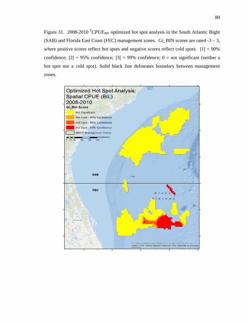
80

Figure 31. 2008-2010 SCPUEBIL optimized hot spot analysis in the South Atlantic Bight

(SAB) and Florida East Coast (FEC) management zones. Gi_BIN scores are rated -3 – 3,

where positive scores reflect hot spots and negative scores reflect cold spots. 1 = 90%

confidence; 2 = 95% confidence; 3 = 99% confidence; 0 = not significant (neither a

hot spot nor a cold spot). Solid black line delineates boundary between management

zones.

81

in each management zone (Figure 31). The smaller hot spot (5,009 km2) is situated over

the northeastward portion of the CPUESWOr hot spot in the SAB, and the larger one

(10,952 km2) is a narrow band which slightly overlaps the fishing effort hot spot in the

FEC on its western boundary and continues eastward across the Blake Plateau nearing the

continental slope.

Interestingly, when the 2008-2010 subsets are broken down and examined year by

year, the fishing effort hot spot in the SAB disappears (Figures 32A-C). Additionally,

instead of a stationary fishing effort hot spot, a westward movement is observed across

the Blake Plateau indicating that vessels are concentrating fishing efforts in different

locations within the target species geographic range through time. Similarly, CPUEBIL

and SCPUEBIL hot spots exhibit westward movement across the Black Plateau (Figures

33A-C and Figures 34A-C, respectively). Istiophorid billfish and tunas are generally

targeted in epipelagic waters (upper 200 m or 650 ft) and are occasionally seen breaking

the surface feeding on shoals of bait fish. Therefore, although not the target species, PLL

vessels may gauge the relative movement of billfish as a tool to increase their chances of

landing the target species, including swordfish which occupy mesopelagic depths during

the day. Adversely, all the CPUESWOr hot spots were identified in the SAB and were

relatively stationary through time (Figures 35A-C).

82

Figure 32A. 2008 Fishing effort distribution optimized hot spot analysis in the South

Atlantic Bight (SAB) and Florida East Coast (FEC) management zones. Gi_BIN scores

are rated -3 – 3, where positive scores reflect hot spots and negative scores reflect cold

spots. 1 = 90% confidence; 2 = 95% confidence; 3 = 99% confidence; 0 = not

significant (neither a hot spot nor a cold spot). Solid black line delineates boundary

between management zones.

83

Figure 32B. 2009 Fishing effort distribution optimized hot spot analysis in the South

Atlantic Bight (SAB) and Florida East Coast (FEC) management zones. Gi_BIN scores

are rated -3 – 3, where positive scores reflect hot spots and negative scores reflect cold

spots. 1 = 90% confidence; 2 = 95% confidence; 3 = 99% confidence; 0 = not

significant (neither a hot spot nor a cold spot). Solid black line delineates boundary

between management zones.

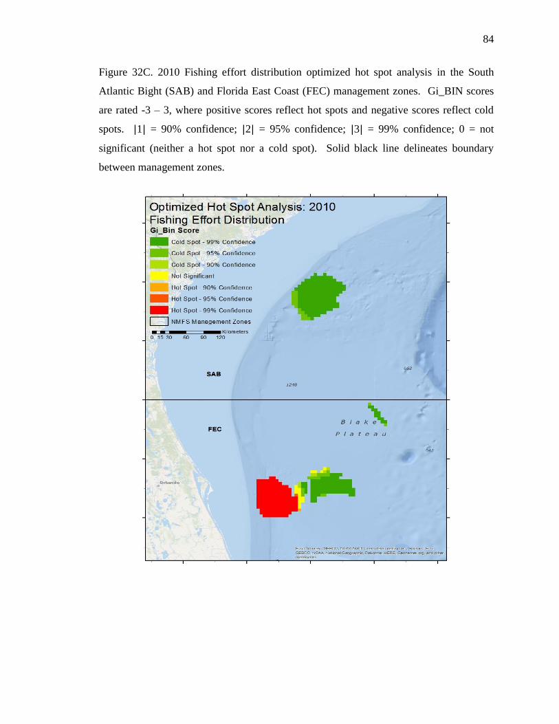
84

Figure 32C. 2010 Fishing effort distribution optimized hot spot analysis in the South

Atlantic Bight (SAB) and Florida East Coast (FEC) management zones. Gi_BIN scores

are rated -3 – 3, where positive scores reflect hot spots and negative scores reflect cold

spots. 1 = 90% confidence; 2 = 95% confidence; 3 = 99% confidence; 0 = not

significant (neither a hot spot nor a cold spot). Solid black line delineates boundary

between management zones.

85

Figure 33A. 2008 CPUEBIL optimized hot spot analysis in the South Atlantic Bight

(SAB) and Florida East Coast (FEC) management zones. Gi_BIN scores are rated -3 – 3,

where positive scores reflect hot spots and negative scores reflect cold spots. 1 = 90%

confidence; 2 = 95% confidence; 3 = 99% confidence; 0 = not significant (neither a

hot spot nor a cold spot). Solid black line delineates boundary between management

zones.

86

Figure 33B. 2009 CPUEBIL optimized hot spot analysis in the South Atlantic Bight

(SAB) and Florida East Coast (FEC) management zones. Gi_BIN scores are rated -3 – 3,

where positive scores reflect hot spots and negative scores reflect cold spots. 1 = 90%

confidence; 2 = 95% confidence; 3 = 99% confidence; 0 = not significant (neither a

hot spot nor a cold spot). Solid black line delineates boundary between management

zones.

87

Figure 33C. 2010 CPUEBIL optimized hot spot analysis in the South Atlantic Bight

(SAB) and Florida East Coast (FEC) management zones. Gi_BIN scores are rated -3 – 3,

where positive scores reflect hot spots and negative scores reflect cold spots. 1 = 90%

confidence; 2 = 95% confidence; 3 = 99% confidence; 0 = not significant (neither a

hot spot nor a cold spot). Solid black line delineates boundary between management

zones.

88

Figure 34A. 2008 SCPUEBIL optimized hot spot analysis in the South Atlantic Bight

(SAB) and Florida East Coast (FEC) management zones. Gi_BIN scores are rated -3 – 3,

where positive scores reflect hot spots and negative scores reflect cold spots. 1 = 90%

confidence; 2 = 95% confidence; 3 = 99% confidence; 0 = not significant (neither a

hot spot nor a cold spot). Solid black line delineates boundary between management

zones.

89

Figure 34B. 2009 SCPUEBIL optimized hot spot analysis in the South Atlantic Bight

(SAB) and Florida East Coast (FEC) management zones. Gi_BIN scores are rated -3 – 3,

where positive scores reflect hot spots and negative scores reflect cold spots. 1 = 90%

confidence; 2 = 95% confidence; 3 = 99% confidence; 0 = not significant (neither a

hot spot nor a cold spot). Solid black line delineates boundary between management

zones.

90

Figure 34C. 2010 SCPUEBIL optimized hot spot analysis in the South Atlantic Bight

(SAB) and Florida East Coast (FEC) management zones. Gi_BIN scores are rated -3 – 3,

where positive scores reflect hot spots and negative scores reflect cold spots. 1 = 90%

confidence; 2 = 95% confidence; 3 = 99% confidence; 0 = not significant (neither a

hot spot nor a cold spot). Solid black line delineates boundary between management

zones.

91

Figure 35A. 2008 CPUESWOr optimized hot spot analysis in the South Atlantic Bight

(SAB) and Florida East Coast (FEC) management zones. Gi_BIN scores are rated -3 – 3,

where positive scores reflect hot spots and negative scores reflect cold spots. 1 = 90%

confidence; 2 = 95% confidence; 3 = 99% confidence; 0 = not significant (neither a

hot spot nor a cold spot). Solid black line delineates boundary between management

zones.

92

Figure 35B. 2009 CPUESWOr optimized hot spot analysis in the South Atlantic Bight

(SAB) and Florida East Coast (FEC) management zones. Gi_BIN scores are rated -3 – 3,

where positive scores reflect hot spots and negative scores reflect cold spots. 1 = 90%

confidence; 2 = 95% confidence; 3 = 99% confidence; 0 = not significant (neither a

hot spot nor a cold spot). Solid black line delineates boundary between management

zones.

93

Figure 35C. 2010 CPUESWOr optimized hot spot analysis in the South Atlantic Bight

(SAB) and Florida East Coast (FEC) management zones. Gi_BIN scores are rated -3 – 3,

where positive scores reflect hot spots and negative scores reflect cold spots. 1 = 90%

confidence; 2 = 95% confidence; 3 = 99% confidence; 0 = not significant (neither a

hot spot nor a cold spot). Solid black line delineates boundary between management

zones.

94

Temporal trends in SCPUESWOr hot spots were less obvious and required closer

examination. In 2008, the SCPUESWOr hot spot (Figure 36A) was narrow in latitude and

nearly spanned across the entire area of observed fishing effort in the FEC. In 2009, that

hot spot (Figure 36B) shifted slightly westward and reduced in size. Then in 2010, the

hot spot further reduced in size and shifted slightly eastward from its 2009 location

(Figure 36C). Additionally, a fair-sized SCPUESWOr hot spot appears in the northward

portion of observed fishing effort in the SAB in 2009, and then in 2010 that hot spot

substantially reduces in size and migrates southwest along the shelf break. These types

of trends reflect the relative shift in hot spot location through time most likely attributed

to inter-annual fluctuations in physical and biological parameters, such as ocean currents

and plankton blooms. Although the general location of the hot spots are the same (e.g., in

waters above the Blake Plateau, or within the FEC), understanding and even anticipating

the small-scale changes in hot spot location can have large economic impacts on the

fishery.

95

Figure 36A. 2008 SCPUESWOr optimized hot spot analysis in the South Atlantic Bight

(SAB) and Florida East Coast (FEC) management zones. Gi_BIN scores are rated -3 – 3,

where positive scores reflect hot spots and negative scores reflect cold spots. 1 = 90%

confidence; 2 = 95% confidence; 3 = 99% confidence; 0 = not significant (neither a

hot spot nor a cold spot). Solid black line delineates boundary between management

zones.

96

Figure 36B. 2009 SCPUESWOr optimized hot spot analysis in the South Atlantic Bight

(SAB) and Florida East Coast (FEC) management zones. Gi_BIN scores are rated -3 – 3,

where positive scores reflect hot spots and negative scores reflect cold spots. 1 = 90%

confidence; 2 = 95% confidence; 3 = 99% confidence; 0 = not significant (neither a

hot spot nor a cold spot). Solid black line delineates boundary between management

zones.

97

Figure 36C. 2010 SCPUESWOr optimized hot spot analysis in the South Atlantic Bight

(SAB) and Florida East Coast (FEC) management zones. Gi_BIN scores are rated -3 – 3,

where positive scores reflect hot spots and negative scores reflect cold spots. 1 = 90%

confidence; 2 = 95% confidence; 3 = 99% confidence; 0 = not significant (neither a

hot spot nor a cold spot). Solid black line delineates boundary between management

zones.

98

Comparing SCPUE to other spatial CPUE metrics’

Indices of relative abundance (i.e., CPUE) have played a pivotal role in fisheries

management. HMS fishery management relies heavily on fishery-dependent data

because reliable fishery-independent data are costly and difficult to collect (Maunder and

Punt 2004). Consequently, multiple standardization techniques have been proposed

which attempt to remove or minimize the effects of variables not attributed to abundance.

Today, most standardization techniques detect temporal trends in abundance; however, it

is widely understood that a true unbiased index of relative abundance must incorporate

both temporal and spatial structure (Hilborn and Walters 1992).

Majority of peer-reviewed literature that address spatial and temporal analysis for

HMS stock assessments either, (a) attempt to improve current standardization techniques

which aim to remove bias introduced by spatial and temporal variation in stock

abundance (e.g., Verdoit et al. 2003), (b) incorporate a spatial component into current

GLMs (e.g., Nishida and Chen 2004), (c) characterize spatial distribution of a fish

population and/or fishing effort from spatially adjusted CPUE (e.g., Jurado-Monlina et al.

2011; Langley, 2006), or a combination of these approaches (e.g., Glaser et al. 2011).

However, this study is the first to explicitly incorporate a spatial component derived

directly from fishing location at the individual set level within the nominal CPUE for

commercially managed pelagic HMS.

A similar study by Langley (2004) developed a spatially-based CPUE for purse

seine-captured skipjack from the west-central Pacific Ocean using the following formula,

CPUEm ∑ ( i

i

i i)

(8)

where CPUEm is the monthly CPUE index; nclust is the number of qualifying clusters in

the month (m); catchi is the total skipjack catch (in metric tons) from clusteri,m; efforti is

the total number of days fished (including searching) by vessels within clusteri,m; areai is

the area (km2) of clusteri,m; and daysi is the duration over which fishing occurred

(calendar days) in clusteri,m. Here, a cluster analysis was conducted using point data do

identify the principal fishing areas for each month. Subsequent CPUEm indices were

99

then calculated using the aggregated skipjack catch, effort, area (of the cluster) and

fishing days within each qualifying cluster. Therefore, Langley’s CPUEm metric does

not explicitly incorporate spatial data on an individual set level, but rather uses the area of

increased fishing effort in the nominal CPUE metric. Additionally, results showed that

the magnitude of variation in the nominal CPUE indices derived from the same catch and

effort data, although similar to CPUEm indices, was considerably less. The opposite is

observed with SCPUE compared to the current nominal CPUE (i.e., 95% of

SCPUE

values were < 0.174, max value = 1.73; 58% of CPUE values < 9.58, max value = 95.8).

Langley (2004) discusses briefly that the alternative methods described for interpreting

catch and effort data are based on the spatial extent of primary fishing location and that

further development of this spatially-based approach may lead to a more reliable index of

stock abundance. Similarly, the relationship between SCPUE and true stock abundance is

limited by the spatial extent of observed fishing effort within the species’ geographic

range.

A second similar study by Courtney and Sigler (2007) analyzed trends in area-

weighted CPUE of Pacific sleeper sharks Somniosus pacificus in the Northeast Pacific

Ocean following the methods previously implemented for sablefish longline surveys by

Sasaki (1985), Sigler and Fujioka (1988), Sigler and Zenger (1989) and Zenger and

Sigler (1992). Here, CPUE was calculated as the number of Pacific sleeper sharks caught

per hachi (a “hachi” is a standardized unit of effort for the sablefish longline survey and

consists of a 100 m line with 45 circle hooks spaced 2 m apart on 1.2 m gangions with 5

m of line left bare on each end of the hachi) for each region (r), station (j), and depth (k).

Area-weighted CPUE was then calculated primarily using the following equation:

RPNrj = ∑ (9)

where CPUE is multiplied by the estimated bottom area (Ark; km2) within each region and

depth combination for each station and summed across depth strata resulting in an

independent estimate of Pacific sleeper shark relative population numbers (RPNs).

Station RPNs were then averaged within survey regions to obtain regional RPNs (RPNr),

which were in turn summed within regulatory areas to provide regulatory area RPNs

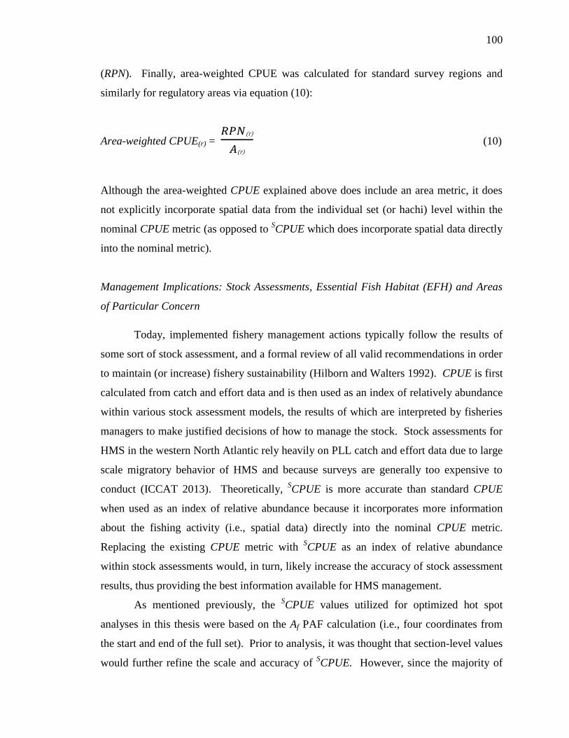
100

(RPN). Finally, area-weighted CPUE was calculated for standard survey regions and

similarly for regulatory areas via equation (10):

Area-weighted CPUE(r) =

(10)

Although the area-weighted CPUE explained above does include an area metric, it does

not explicitly incorporate spatial data from the individual set (or hachi) level within the

nominal CPUE metric (as opposed to SCPUE which does incorporate spatial data directly

into the nominal metric).

Management Implications: Stock Assessments, Essential Fish Habitat (EFH) and Areas

of Particular Concern

Today, implemented fishery management actions typically follow the results of

some sort of stock assessment, and a formal review of all valid recommendations in order

to maintain (or increase) fishery sustainability (Hilborn and Walters 1992). CPUE is first

calculated from catch and effort data and is then used as an index of relatively abundance

within various stock assessment models, the results of which are interpreted by fisheries

managers to make justified decisions of how to manage the stock. Stock assessments for

HMS in the western North Atlantic rely heavily on PLL catch and effort data due to large

scale migratory behavior of HMS and because surveys are generally too expensive to

conduct (ICCAT 2013). Theoretically, SCPUE is more accurate than standard CPUE

when used as an index of relative abundance because it incorporates more information

about the fishing activity (i.e., spatial data) directly into the nominal CPUE metric.

Replacing the existing CPUE metric with SCPUE as an index of relative abundance

within stock assessments would, in turn, likely increase the accuracy of stock assessment

results, thus providing the best information available for HMS management.

As mentioned previously, the SCPUE values utilized for optimized hot spot

analyses in this thesis were based on the Af PAF calculation (i.e., four coordinates from

the start and end of the full set). Prior to analysis, it was thought that section-level values

would further refine the scale and accuracy of SCPUE. However, since the majority of

101

the catch usually comes from one or a few sections and is rarely proportional throughout

the set, section-level SCPUE are extremely variable and can further skew proportionality

interpretations when used as an index for relative abundance. However, it is

acknowledged that section coordinates do provide a more accurate visual of the area

fished by the gear during the soak. Therefore, if captain and observer reporting

requirements were to include section coordinates then Afs would be the preferred spatial

component for SCPUE.

Additionally, HMS management groups can benefit from monitoring the spatio-

temporal relationship between fishing effort and SCPUE hot spot locations. Based on

these results, SCPUE can be very insightful when delineating boundaries around existing

Time-Area Closures (TAC), Marine Protected Areas (MPA), and Essential Fish Habitat

(EFH). These hot spots can also help identify potential areas for concern for both target

and non-target species that would not otherwise be identified by current spatial

representation methods used for HMS management. Historically, animal interactions are

spatially referenced using the starting location of PLL sets in which a specific interaction

was observed (ICCAT 2013; APLTRP 2014). Since a single PLL set frequently exceeds

30 miles, this method rarely accurately identifies where an interaction took place in

space. Using the new SCPUE, in addition to utilizing spatial information within the

metric itself, HMS fishery managers can more accurately identify where an observed

animal interaction occurred within the boundaries of the PAF. Therefore, not only could

the described methods identify new areas for protection, but fishery managers may also

wish to redefine current TAC, MPA, and EFH boundaries.

Conclusion and Future Research

These results are by no means a “silver bullet” for relative abundance indices.

For effective fisheries management, SCPUE should only be used in the context of other

data and information relating to the spatial distribution of fish and fishing effort. The

most effective use of SCPUE as a tool for fisheries management is unclear and warrants

further investigation. As explained by Hilborn and Walters (1992) and reiterated by

Langley (2004), if SCPUE hot spot results were disseminated to commercial fishermen to

better target and avoid particular species, it is likely that fishing effort would become

102

increasingly concentrated in and around the hot spots identified for target species,

therefore leading to “hyperstability” interpretations from nominal SCPUE indices.

Conversely, if SCPUE hot spot results were retained by fisheries managers solely for

monitoring particular areas of concern, then fishermen would not have the best scientific

information available in regards to avoiding bycatch and increasing target catch.

SCPUE, and subsequent relative abundance indices for HMS, remain heavily

reliant on fisheries dependent data. As discussed previously, due to extreme high costs

associated with PLL surveys and the highly migratory behavior of these fishes, the lack

of fishery independent data sources will likely remain a limitation to HMS stock

assessments and successive management actions. A number of other assumptions have to

be made when applying the described methods above which are primarily related to

changes in catchability and the interactions between fishing fleet dynamics and target

species populations. More than likely, these assumptions will be violated to some degree.

However, it remains highly probable that SCPUE can significantly reduce the biases

introduced when used as an index for relative abundance within HMS stock assessments

compared to the current methodology.

The spatio-temporal analyses examined in this thesis are case-specific examples

of how GPS data that is currently recorded by all NMFS fisheries observers could be

utilized to create a new SCPUE metric thus eliminating the assumption that all parts of

species geographic have the same proportion of individuals. SCPUE, when used as an

index for relative abundance, is more accurate than the conventional CPUE because it

incorporates spatial information directly obtained from the fishing location. Additionally,

SCPUE can be visualized using GIS software to identify hot spots where target and non-

target species aggregate. These smaller, more defined hot spots would not have

otherwise been identified using the current spatial referencing method for HMS which

uses the starting location at the start of PLL sets. It is important to note that fishing effort

was not conducted in all locations of the study area, nor was effort conducted equally

across all management zones. Fishing effort distribution is a product of accessibility, and

captain experience and knowledge of the fishery which is passed on most often by word

of mouth. Therefore, complete coverage of HMSs geographic range remains a limitation

to HMS management.

103

The results of this thesis warrant continued research with spatial CPUE, derived

from observer based fishery-dependent data, as an index for relative abundance within

stock assessment models. However, it would be advisable for NMFS to apply the

described methods to their extensive records of archived captain-reported logs and

observer data from the western North Atlantic PLL fleet. The results of such an analysis

would be applicable to the entire fleet. Additionally, SCPUE indices of relative

abundance could be used within current integrated stock assessment models, the results

of which could be compared to stock assessment results that use the standard CPUE

metric. Further still, stock abundance could be forecasted according to various

management regimes using SCPUE as an index of relative abundance and compared to

current management regimes and stock abundance projections. Inevitably, the results of

stock assessment models using SCPUE as an index of relative abundance would most

likely differ from current results using standard CPUE, thus leading to different

management recommendations.

Other research efforts should focus on the spatio-temporal trends in hot spot

location with physical parameters including ocean-atmosphere oscillations (i.e., Pacific

Decadal Oscillations and El Niño Southern Oscillations), ocean gyres, and smaller scale

seasonal parameters such as SST, current speed and strength, and plankton blooms.

Examining maps of hot spot location overlaid with remote sensing data (e.g., SST or

chlorophyll a) for past time periods would provide an opportunity to forecast future

SCPUE hot spots and add insight to where vessels will most likely concentrate fishing

effort. Various kriging (interpolation) methods may also be applicable for further hot

spot analysis to provide information on hot spot location beyond the range of observed

fishing effort.

104

Works Cited:

Atlantic Highly Migratory Species Management Division (HMSMD). 2014. National

Oceanic and Atmospheric Administration (NOAA) National Marine Fisheries

Service (NMFS). Office of Sustainable Fisheries (OSF). Retrieved via:

http://www.nmfs.noaa.gov/sfa/hms/

Arreguín-Sánchez, Francisco. 1996. Catchability: a key parameter for fish stock

assessment. Reviews in Fish Biology and Fisheries. 6:221-242

Beverton, R.J.H. and Holt, S.J. 1957. On the Dynamics of Exploited Fish Populations.

HMSO, London.

Bigelow, K.A., Kerstetter, D.W., Dancho, M.G. and Marchetti, J.A. 2012. Catch rates

with variable strength circle hooks in the Hawaii-based tuna longline fishery.

Bulletin of Marine Science. Rosensteil School of Marine and Atmospheric Science f

the University of Miami. 88(3):425-447

Campbell, Robert A. 2004. CPUE standardisation and the construction of indices of atock

abundance in a spatially varying fishery using general linear models. Fisheries

Research. 70:209-227

Can, M. F., Mazlum, Y., Demirci, A., and Aktas, M. 2004. The catch composition and

catch per unit swept area (CPUE) of Penaeid shrimps in the bottom trawls from

Iskenderun Bay, Turkey. Turkish Journal of Fisheries and Aquatic Sciences. 4:87-91

Carruthers, T.R., McAllister, M.K., and Ahrens, R.N.M. 2010. Simulating spatial

dynamics to evaluate methods of deriving abundance indices for tropical tunas.

Canadian Journal of Fisheries and Aquatic Science. 67:1409-1427

Cooke, J.G. and Beddinton, J.R. 1984. The relationship between catch rates and

abundance in Fisheries. IMA journal of Mathematics Applied in Medicine and

Bioogy. 1:391-405

Cooper, Andrew B. 2006. A guide to fisheries stock assessment: from data to

recommendation. Department of Natural Resources. Retrieved via Southeast

Fisheries Science Center.

Cudmore, W.W. 2009. The Decline of Atlantic Cod: a case study. Northwest Center for

Sustainable Resources. Salem, OR.

Electronic Code of Federal Regulations. 2013. Retrieved via: www.ecfr.gov

105

ESRI (Environmental Systems Resource Institute). 2014. ArcMap 10.2. ESRI, Redlands,

California.

ESRI (Environmental Systems Resource Institute). 2014. ArcGIS Online Resources for

server 10.2.X. Received via: http://resources.arcgis.com/en/home/

FSEIC Description of the pelagic longline fishery for Atlantic HMS. 1999. National

Oceanic and Atmospheric Administration (NOAA) National Marine Fisheries

Service (NMFS). Retrieved via:

http://www.nmfs.noaa.gov/sfa/hms/related_topics/bycatch/documents/fseis_final_sec

tion_6.pdf

Gillis, D.M. and Peterman, R.M. 1998. Implications of Interference among fishing

vessels and the ideal free distribution to the interpretation of CPUE. Canadian

Journal of Fisheries and Aquatic Science. 55:37-46

Glaser, S.M., Ye, H., Maunder, M., MacCall, A., Fogarty, M., and Sugihara, G. 2011.

Detecting and forecasting complex nonlinear dynamics in spatially structured catch-

per-unit-effprt time series for North Pacific albacore. Canadian Journal of Fisheries

and Aquatic Science. 68: 400-412

Gunderson, D.R. 1993. Surveys of fisheries resources. John Wiley & Sons, New York.

p.248

Highly Migratory Species Commercial Compliance Guide. 2014. National Marine

Fisheries Service. National Ocean and Atmospheric Administration. U. S.

Department of Commerce. p 11.

Harley, Shelton J., Ransom A. Myers, and Alistair Dunn. 2001. Is catch-per-unit-effort

proportional to abundance. Canadian Journal of Fisheries and Aquatic Science.

58:1760-1772

Final Consolidated Atlantic Highly Migratory Species Fishery Management Plan

(HMSFMP). 2006. National Oceanic and Atmospheric Administration’s National

Marine Fisheries Service (NOAA’s NMFS). Office of Sustainable Fisheries. Highly

Migratory Species Management Division.

Hilborn, R., and Walters, C.J. 1987. A general model for simulation of stock and fleet

dynamics in spatially heterogeneous fisheries. Canadian Journal of Fisheries and

Aquatic Science. 44:1366-1369

106

Hilborn, R. and Walters, C.J. 1992. Quantitative Fisheries Stock Assessment: choice,

dynamics and uncertainty. Chapman & Hall, London.

Hoey, J.J. and Moore, N. 1999. Captains report. Multispecies characteristics for the U.S.

Atlantic pelagic longline fishery. National Fisheries Institute Report to NOAA,

National Marine Fisheries Service, Silver Spring, Md., USA.

Hutchings, J.A. 1996. Spatial and temporal variation in the densities of Northern Cod and

a review of hypotheses for the stock collapse. Canadian Journal of Fisheries and

Aquatic Science. 53: 943-962

International Commission for the Conservation of Atlantic Tunas (ICCAT). 2013. ICCAT

Manual. International Commission for the Conservation of Atlantic Tuna. In: ICCAT

Publications [on-line]. Updated 2013.

Jennings, S., Kaiser, M.J. and Reynolds, J.D. 2001. Marine Fisheries Ecology. Blackwell

Publishing. 98-106

Jurado-Molina, J., Bigelow, K., Hoyle, S., Nicol, S., and Briand, K. 2011. Developing a

spatially adjusted CPUE for the albacore fishery in the South Pacific. Western and

Central Pacific Fisheries Commission. 9-17 August 2011, Pohnpei, Federated States

of Micronesia.

Kerstetter, D. 2011. Pilot Project: Evaluating the Effects of Circle Hooks on Catch Rates

within Two Pelagic Longline Time-Area Closures. Final report to NOAA, contract

number 8404-S-006

Kerstetter, D.W. and Graves, J.E. 2006. Effects of circle versus J-style hooks on target

and non-target species in a pelagic longline fishery. Fisheries Research. 80: 239-250

Langley, A. 2004. A spatially based analysis of purse-seine skipjack CPUE from

unassociated sets in the equatorial area of the WCPO, including the development of

an oceanographic model for the fishery. 17th

meeting of the Standing Committee on

Tuna and Billfish. Majuro, Marshall Islands, 9-18 August 2004.

Langley, A. 2006. Spatial and temporal trends in yellowfin and bigeye longline CPUE for

the Japanese fleet in WCPO. Western Central Pacific Fisheries Commission. Manila

Philippines, 7-18 August 2006.

107

Lynch, Patrick D., Hyle W. Shertzer, and Robert J. Latour. 2012. Performance of

methods used to estimate indices of abundance for highly migratory species.

Fisheries Research 125-126:27-39

Magnuson-Stevens Fisheries Conservation and Management act (MSA). 1996. Public law

94-265. Retrieved February 22, 2013 via: http://www.nmfs.noaa.gov/sfa/magact/

Magnuson-Stevens Reauthorization Act (MSRA). 2008. National Oceanic and

Atmospheric Administration. Retrieved via:

http://www.noaa.gov/factsheets/new%20version/magstevens.pdf

Maunder, M.N. and Punt, A.E. 2004. Standardizing catch and effort data: a review of

recent approaches. Fisheries Research. 70:141-159

Maunder, Mark N., Sibert, John R., Alain Fonteneau, John Hampton, Pierre Kleiber, and

Sherlton J. Harley. 2006. Interpreting catch per unit effort data to assess the status of

individual stocks and communities. ICES Journal of Marine Science. 63:1373-1385

Maury, O., Gascuel, D., Marsac, F., Fonteneau, A., and De Rosa, A.L. 2001. Hierarchical

interpretation of nonlinear relationships linking yellowfin tuna (Thunnus albacares)

distribution to the environment in the Atlantic Ocean. Canadian Journal of Fisheries

and Aquatic Science. 58:458-469

Melvin, E.F. 2000. Streamer lines to reduce seabird bycatch n longline fisheries.

Washington Sea Grant. National Oceanic and Atmospheric Administration.

Microsoft. (2010). Microsoft Excel [computer software]. Redmond, Washington:

Microsoft.

Moustakas, A., Silvert, W., and Dimitromanolakis, A. 2006. A spatially explicit learning

model of migratory fish and fishers for evaluating closed areas. Ecological

Modeling. 192:245-258

Nishida, Tom and Chen, Ding-Geng. 2004. Incorporating spatial autocorrelation into the

general linear model with an application to the yellowfin tuna (Thunnus albacares)

longline CPUE data. Fisheries Research. 70:265-274

Pelagic Longline Take Reduction Plan (PLTRP). 2006. National Oceanic and

Atmospheric Association. National Marine Fisheries Service.

108

Pelagic Observer Program. 2014. National Oceanic and Atmospheric Administration.

National Marine Fisheries Service. Southeast Fisheries Science Center. Retrieved

via: http://www.sefsc.noaa.gov/fisheries/observers/pelagic.htm

Stock Assessment and Fishery Evaluation (SAFE) Report for Atlantic Highly Migratory

Species. 2014. National Oceanic and Atmospheric Administration, National Marine

Fisheries Service. Atlantic Highly Migratory Species Management Division.

Sullivan, P.J. 1992. CPUE and the IVQ program. Report of Assessment and Research

Activities. International Pacific Halibut Commission. p.79-140

Team, R. D. C. 2010. R: A language and environment for statistical computing. Vienna,

Austria: R Foundation for Statistical Computing. Retrieved via: http://www.R-

project.org

Verdoit, M, Pelletier, D and Bellail, R. 2003. Are commercial logbook and scientific

CPUE data useful for characterizing the spatial and seasonal distribution of exploited

population? The case of the Celtic Sea whiting. Aquatic Living Resources. 16:467-

485

Walters, Carl. 2003. Folly and fantasy in the analysis of spatial catch rate data. Canadian

Journal of Fisheries and Aquatic Science. 60:1433-1436

Wang, S.P., Maunder, M.N., Aires-da-Silva, A. 2009. Implications of model and data

assumptions: an illustration including data for the Taiwanese longline fishery into the

eastern Pacific Ocean bigeye tuna (Thunnus obesus) stock assessment. Fisheries

Research. 97:118-126

Ward, P. and Hindmarsh, S. 2007. An overview of historical changes in the fishing gear

and practices of pelagic longliners, with particular reference to Japan’s Pacific fleet.

Rev Fish Biology Fisheries. 17:501-516

Watson, J.W. and Kerstetter, D.W. 2006. Pelagic longline fishing gear: a brief history and

review of research efforts to improve selectivity. Marine Technology Society

Journal. 40 (3)

109

APPENDIX

I. Trip Summary Log

110

II. Longline Gear Log

111

III. Longline Haul Log

112

IV. Animal Log

113

V. Animal Tally Log created for data entry efficiency