a broadband fast multipole accelerated boundary element method …ramani/pubs/gumerovduraiswa… ·...

A broadband fast multipole accelerated boundary elementmethod for the three dimensional Helmholtz equation

Nail A. Gumerova�,b� and Ramani Duraiswamib�,c�

Perceptual Interfaces and Reality Laboratory, Institute for Advanced Computer Studies,University of Maryland, College Park, Maryland 20742

�Received 2 January 2008; revised 3 October 2008; accepted 10 October 2008�

The development of a fast multipole method �FMM� accelerated iterative solution of the boundaryelement method �BEM� for the Helmholtz equations in three dimensions is described. The FMM forthe Helmholtz equation is significantly different for problems with low and high kD �where k is thewavenumber and D the domain size�, and for large problems the method must be switched betweenlevels of the hierarchy. The BEM requires several approximate computations �numerical quadrature,approximations of the boundary shapes using elements�, and these errors must be balanced againstapproximations introduced by the FMM and the convergence criterion for iterative solution. Thesedifferent errors must all be chosen in a way that, on the one hand, excess work is not done and, onthe other, that the error achieved by the overall computation is acceptable. Details of translationoperators for low and high kD, choice of representations, and BEM quadrature schemes, allconsistent with these approximations, are described. A novel preconditioner using a low accuracyFMM accelerated solver as a right preconditioner is also described. Results of the developed solversfor large boundary value problems with 0.0001�kD�500 are presented and shown to performclose to theoretical expectations. © 2009 Acoustical Society of America. �DOI: 10.1121/1.3021297�

PACS number�s�: 43.55.Ka, 43.20.Fn, 43.28.Js �NX� Pages: 191–205

I. INTRODUCTION

Boundary element methods �BEMs� have long been con-sidered as a very promising technique for the solution ofmany problems in computational acoustics governed by theHelmholtz equation. They can handle complex shapes, leadto problems in boundary variables alone, and lead to simplermeshes where the boundary alone must be discretized ratherthan the entire domain. Despite these advantages, one issuethat has impeded their widespread adoption is that they leadto linear systems with dense and possibly nonsymmetric ma-trices. As the domain size increases to many wavelengths,the number of variables in the discretized problem, N, shouldincrease correspondingly to satisfy the Nyquist sampling cri-terion. For a problem with N unknowns, a direct solutionrequires O�N3� solution cost and storage of O�N2�. Use ofiterative methods does not reduce the memory but can reducethe cost to O�NiterN

2� operations, where Niter is the number ofiterations required, and the O�N2� per iteration cost arisesfrom the dense matrix-vector product. In practice this is stillquite large. An iteration strategy that minimizes Niter is alsoneeded. Other steps in the BEM are also expensive, such asthe computation of the individual matrix elements, whichrequire quadrature of nonsingular, weakly singular, or hyper-singular functions. To reduce the singularity order andachieve symmetric matrices, many investigators employGalerkin techniques, which lead to further O�N2� integralcomputations. Because of these reasons, the BEM was notused for very large problems. In contrast finite-difference and

a�Electronic mail: [email protected]�Also at Fantalgo, LLC, Elkridge, MD 20751.c�
Electronic mail: [email protected]
J. Acoust. Soc. Am. 125 �1�, January 2009 0001-4966/2009/125�1

finite element methods, despite requiring larger volumetricdiscretizations, have well established iterative solvers and aremore widely used.

The combination of the fast multipole method1 �FMM�and the preconditioned Krylov iterative methods presents apromising approach to improving the scalability of BEMsand is an active area of research. The FMM for potentialproblems allows the matrix-vector product to be performedto a given precision � in O�N� operations and further doesnot require the computation or storage of all N2 elements ofthe matrices, reducing the storage costs to O�N� as well.Incorporating the fast matrix-vector product in a quicklyconvergent iterative scheme allows the system of equationsto be rapidly solved with O�NiterN� cost. The FMM was ini-tially developed for gravity or electrostatic potential prob-lems. Later this method was intensively studied and extendedto the solution of problems arising from the Helmholtz, Max-well, biharmonic, elasticity, and other equations. While theliterature and previous work on the FMM is extensive, rea-sons of space do not permit a complete discussion of theliterature. The reader is referred to Ref. 2 for a comprehen-sive review.

II. FMM AND FMM ACCELERATED BEM FOR THEHELMHOLTZ EQUATION

The FMM and FMM accelerated BEM for the Helm-holtz equation have seen significant work, and several au-thors have recently published on various aspects of theproblem,3–9 and new articles have appeared when this articlewas in review.10 This article presents a FMM accelerated
boundary element solver for the Helmholtz equation that has
© 2009 Acoustical Society of America 191�/191/15/$25.00

the following contributions that distinguish it from previouswork:

• achieves good performance at both low and high frequen-cies by changing the representation used,

• has a quickly convergent iterative scheme via a novel pre-conditioner, which is described here,

• achieves further efficiency by considering the error of thequadrature in the BEM in the overall error analysis of theFMM, and

• uses the Burton–Miller �combined� boundary integral for-mulation for external problems and avoids the problemswith spurious resonances.

A. Error and fast multipole accelerated boundaryelements

During the approximate solution of the Helmholtz equa-tion via the FMM accelerated BEM, the following differentsources of error are encountered:

• geometric error due to the discretization of the surface withmeshes,

• quadrature error in computation of boundary integrals,• matrix-vector product error due to the FMM, and• residue error used as a termination criterion during the

iterative solution process.

One of the contributions of this paper is to consider allthe errors together and design an algorithm that provides therequired accuracy and avoids wasteful computations. Itshould be noted that the error achieved in practice in manyreported simulation error tolerances is quite high, from ahigh of a few percent to at most 10−4 �see, e.g., Refs. 4, 5,and 11�. Many previous FMM/BEM simulations containcomputations that are wasteful of CPU time and memorywhen considering the final error desired or achieved.

B. Resolving calculations over a large range ofwavenumbers

To be accurate, any calculation must resolve the smallestwavelengths of interest, and to satisfy the Nyquist criterion,the discretization must involve at least two points per wave-length. The restriction imposed by this requirement manifestsitself at large frequencies since at lower frequencies the dis-cretization is controlled by the necessity to accurately repre-sent the boundary. Thus, two basic regimes for the FMMBEM are usually recognized in acoustic simulations: thelow-frequency regime and the high-frequency regime. Theseregimes can be characterized by some threshold value �kD�*of the parameter kD, where k is the wavenumber and D is thecomputational domain size. For each of these regimes thecomputational complexity of the FMM exhibits a differentbehavior.12

1. Low-frequency regime

In the low-frequency regime, kD� �kD�*, the per itera-tion step cost of the FMM is proportional to N and not verymuch affected by the value of kD. Here, the most efficient
representation is in terms of spherical multipole wavefunc-
192 J. Acoust. Soc. Am., Vol. 125, No. 1, January 2009 Gumero

tions, and the translation schemes are based on the rotation-coaxial translation-backrotation �RCR� decompositions,12,13

which have O�p3� complexity. Here p2 is the number ofterms in the multipole expansion �p in this regime can beconstant�. Alternately one may use the low-frequency expo-nential forms,14,15 which have the same complexity, but witha different asymptotic constant. The method of function rep-resentation based on sampling of the far-field signaturefunction16 is not stable in this region due to exponentialgrowth of terms in the multipole-to-local translation kernel.

2. High-frequency regime

In the high frequency regime, kD� �kD�*, and the valueof kD heavily affects the cost. Since the wavenumber k isinversely proportional to wavelength and, in practice, five toten points per wavelength are required for accuracy, for asurface-based numerical method �such as the BEM� the prob-lem size N scales as O�kD�2, while for volumetric problems�e.g., for many scatterers distributed in a volume� N scales asO�kD�3. For this regime, the size of the wavefunction repre-sentation, which is O�p2�, must increase as the levels go upin the hierarchical space subdivision, with p proportional tothe size of the boxes at a given level.12 Because of this, thecomplexity of the FMM is heavily affected by the complex-ity of a single translation. It was shown12 that O�p3� schemes�such as the RCR scheme� result in an overall complexity ofthe FMM O�kD�3 for simple shapes and O��kD�3 log�kD��for space-filling surfaces. The use of translation schemes ofO�p4� and O�p5� complexities in this case provides the over-all complexity of the FMM that is slower than the directmatrix-vector product. Where FMM with translationschemes of such complexity have been used with the BEM�e.g., see Ref. 7�, one must recognize that the software isonly usable in the low-frequency regime.

To reach the best scaling algorithm in the high-frequency regime, translation methods based on representa-tions that sample the far-field signature function16 are neces-sary. The translation cost in this case scales as O�p2�, whileat least O�p2 log p� additional operations are needed for thespherical filtering necessary for numerical stabilization of theprocedure. In this case the overall FMM complexity will beO��kD�2 log� �kD�� 1� for simple shapes and O��kD�3�for space-filling shapes.

3. Switch in function representations

As discussed above, different representations are appro-priate for low and high kD. However, even for high kD prob-lems, since the FMM employs a hierarchical decomposition,at the fine levels, the problems behave as a low kD problem.Indeed at the fine levels, parameter ka, where a is a repre-sentative box size, is smaller than �kD�*, and translationsappropriate to the low-frequency regime should be used. Forcoarser levels, ka is large and the high-frequency regimeshould be used, and a combined scheme in which the spheri-cal wavefunction representation can be converted to signa-ture function sample representation is needed. Such a switch
was also suggested and tested recently in Ref. 17. The
v and Duraiswami: Fast multipole method boundary element method

present scheme, however, is different from that of Ref. 17and does not require interpolation/anterpolation.

4. Comparison with volumetric methods

Similarly volumetric methods, such as the finite-difference time domain �FDTD� method for the wave equa-tion, have the requirement that to resolve a simulation theyneed several points per wavelength. Thus for a problem on adomain of size kD, in three dimensions we have N��kD�3,with this restriction being controlling at higher frequencies.Fast iterative methods, e.g., based on multigrid solve thesesystems in constant number of iterations and for a cost ofO�N4/3� per time step. So for a problem with M time steps,we have O�MN4/3�=O�M�kD�4� complexity for the volumet-ric methods �this is based on the discussion in Ref. 18�. Incontrast a fast multipole accelerated BEM, which is precon-ditioned with a preconditioner requiring a constant numberof steps and is solved at M frequencies, can achieve solutionin O�M�kD�2 log �kD�� or O�M�kD�3� steps. However, interms of programming ease the FDTD and finite element TDmethods are much easier to implement, and the precondition-ers developed for them work better. Further they are easier togeneralize to nonisotropic media. Their difficulty in handlinginfinite domains has been largely solved via perfectlymatched layer methods. Accordingly, despite the advantagesprovided by integral equation approaches for the Helmholtzequation, volumetric approaches are popular.

C. Iterative methods and preconditioning

Preconditioning can be very beneficial for fast conver-gence of Krylov subspace iterative methods. Preconditioningfor boundary element matrices is, in general, a lesser studiedissue than for finite-element- and finite-difference-based dis-cretizations. From that theory, it is known that for high wave-numbers preconditioning is difficult and an area of activeresearch. Many conventional preconditioning strategies relyon sparsity in the matrix, and applying them to dense BEMmatrices requires computations that have a formal time ormemory complexity of O�N2�, which negates the advantageof the FMM.

One strategy that has been applied with the FMBEM isthe construction of approximate inverses for each row basedon a local neighborhood of the row. If K neighboring ele-ments are considered, then constructing this matrix has a costof O�NK3�, and there is a similar cost to applying the pre-conditioner at each step.3,4 However such local precondition-ing strategies appear to work well only for low wavenum-bers. Instead in this paper the use of a low accuracy FMMitself as a preconditioner by using a flexible generalizedminimal residual �fGMRES� procedure19 is considered. Thisnovel preconditioner appears to work reasonably at all wave-numbers considered and stays within the required cost.

III. FORMULATION AND PRELIMINARIES

A. Boundary value problem

Consider the Helmholtz equation for the complex valued
potential �,
J. Acoust. Soc. Am., Vol. 125, No. 1, January 2009 Gumerov and D

�2� + k2� = 0, �1�

with real wavenumber k inside or outside finite three dimen-sional �3D� domain V bounded by closed surface S, subjectto mixed boundary conditions

��x��x� + ��x�q�x� = �x�, q�x� =��

�n�x� ,

�2�� + �� 0, x � S .

Here and below all normal derivatives are taken, assumingthat the normal to the surface is directed outward to V. Forexternal problems � is assumed to satisfy the Sommerfeldradiation condition

limr→

�r� ��

�r− ik� = 0, r = �x� . �3�

This means that for scattering problems � is treated as thescattered potential.

Note then that there should be some constraints on sur-face functions ��x�, ��x�, and �x� for existence and unique-ness of the solution. Particularly, if � and � are constant, thisleads to the Robin problem, which degenerates to the Dirich-let or Neumann problem. For �=0 the case of a “sound-soft”boundary is obtained, and for �=0 the “sound-hard” bound-ary case is obtained.

B. Boundary integral equations

The BEM uses a formulation in terms of boundary inte-gral equations whose solution with the boundary conditionsprovides ��x� and q�x� on the boundary and subsequentlydetermines ��y� for any domain point y. This can be done,e.g., using Green’s identity

��y� = L�q� − M��, y � S . �4�

Here the upper sign in the left hand side should be taken forthe internal domain, while the lower sign is for the externaldomain �this convention is used everywhere below�, and Land M denote the following boundary operators:

L�q� = �S

q�x�G�x,y�dS�x� ,

�5�

M�� = �S

��x��G�x,y��n�x�

dS�x� ,

where G is the free-space Green’s function for the Helmholtzequation

G�x,y� =eikr

4�r, r = �x − y� . �6�

In principle, Green’s identity can be also used to providenecessary equations for determination of the boundary valuesof ��x� and q�x�, as in this case for smooth S one obtains

�12��y� = L�q� − M��, y � S , �7�

The well-known deficiency of this formulation is related to� 1 �
possible degeneration of the operators L and M − 2 at cer-
uraiswami: Fast multipole method boundary element method 193

tain frequencies depending on S, which correspond to reso-nances of the internal problem for sound-soft and sound-hardboundaries.20,21 Even though the solution of the externalproblem is unique for these frequencies, Eq. �7� is deficientin these cases. Moreover, for frequencies in the vicinity ofthe resonances, the system becomes poorly conditioned nu-merically. On the other hand, when solving internal problems�e.g., in room acoustics�, the nonuniqueness of the solutionfor the internal problem has a physical meaning, as there areresonances.

In any case, Eq. �7� can be modified to avoid the artifactof degeneracy of boundary operators when solving the cor-rectly posed problems �1�–�3�. This can be done using dif-ferent techniques, including direct and indirect formulations,introduction of some additional field points, etc. A directformulation based on the integral equation combiningGreen’s and Maue’s identities, which is the method proposedby Burton and Miller20 for sound-hard boundaries, is used.The Maue identity is

�12q�y� = L��q� − M��, y � S , �8�

where

L��q� = �S

q�x��G�x,y��n�y�

dS�x� ,

�9�

M�� =�

�n�y��S

��x��G�x,y��n�x�

dS�x� .

Multiplying Eq. �8� by some complex constant and sum-ming with Eq. �7�, one obtains

�12 ��y� + q�y�� = �L + L��q� − �M + M�� . �10�

Burton and Miller20 proved that it is sufficient to haveIm� ��0 to guarantee the uniqueness of the solution for theexternal problem.

C. Combined equation

Using the boundary conditions, the system of equations�2� and �10� can be reduced to a single linear system forsome vector of elemental or nodal unknowns ��,

A�� = c , �11�

which is convenient for computations. The boundary opera-tor A and functions � and c can be constructed followingstandard BEM procedures. They can be expressed as

A�� = �L + L��u�� − �M + M��u� �12 �u + u�� ,

�12�c = �L + L��b�� − �M + M��b� �

12 �b + b�� ,

where u and u� are related to the unknown �, and b and b�are related to the knowns. For example, for the Neumannproblem u=�, u�=0, while b�=q and b=0.

D. Discretization

Boundary discretization leads to approximation of
boundary functions via finite vectors of their surface samples

and integral operators via matrices acting on these vectors.For example, if the surface is discretized by a mesh with Mpanels �elements�, Sl�, and N vertices, x j, and integrals overthe boundary elements are computed, one obtains

L�q��xl�c�� = �

l�=1

M �Sl�

q�x�G�x,xl�c��dS�x�

�l�=1

M

Lll�ql�, l = 1, . . . ,M ,

�13�

ql� = q�xl��c��, Lll� = �

Sl�

G�x,xl�c��dS�x� ,

where xl��c� is the center of the l�th element, and for compu-

tations of matrix entries Lll� one can use well-known quadra-tures, including those for singular integrals.21,22 The aboveequation is for the case of panel collocation, while analogousequations can be derived for vertex collocation. Similar for-mulas can be used for other operators. Note that to accuratelycapture the solution variation at the relevant length scales,the discretization should satisfy krmax�1, where rmax is themaximum size of the element. In practice, discretizationsthat provide several elements per wavelength usually achievean accuracy consistent with the other errors of the BEM. Theabove method of discretization with collocation either at thepanel centers or vertices was implemented and tested. Dis-cretization of the boundary operators reduces problem �11� toa system of linear equations.

E. Iterative methods

Different iterative methods can be tried to solve Eq.�11�, which has a nonsymmetric dense complex valued ma-trix A. Any iterative method requires computation of thematrix-vector product A�x�, where �x� is some input vector.The method used in the present algorithm is the fGMRESmethod,19 which has the advantage that it allows use of ap-proximate right preconditioner, which in its turn can be com-puted by executing of the internal iteration loop using un-preconditioned GMRES.23 Choice of the preconditioningmethod must be achieved for a cost that is O�N� or smaller.This flexibility is exploited in the present algorithm.

IV. USE OF THE FAST MULTIPOLE METHOD

The main idea of the use of the FMM for the solution ofthe discretized boundary integral equation is based on thedecomposition of operator A,

A = Asparse + Adense, �14�

where the sparse part of the matrix has only nonzero entriesAlj corresponding to the vertices xl and x j, such that �xl

−x j��rc, where rc is some distance usually of the order ofthe distance between the vertices, whose selection can bebased on some estimates or error bounds, while the densepart has nonzero entries Alj for which �xl−x j��rc. The use ofthe FMM reduces the memory complexity of the overall

2
product to O�N� and the computational complexity to o�N �,

which can be O�N�, O�N log� N�, ��1, or O�N��, ��2,depending on the wavenumber, domain size, effective di-mensionality of the boundary, and translation methodsused.12

A. FMM strategy

The use of the FMM for the solution of boundary inte-gral equations brings a substantial shift in the computationalstrategy. In the traditional BEM the full system matrix mustbe computed to solve the resulting linear system either di-rectly or iteratively. The memory needed to store this matrixis fixed and is not affected by the accuracy imposed on thecomputation of the surface integrals. Even if one usesquadratures with a relatively high number of abscissas andweights to compute integrals over the flat panels in a con-stant panel approximation, the memory cost is the same, andthe relative increase in the total cost is small, as that cost isdominated by the linear system solution.

If one chooses, as done by previous authors using theFMM accelerated BEM �see, e.g., Refs. 5 and 7�, to computenonsingular integrals very accurately in the FMM using ex-pansions of Green’s function, such as

G�x,xl�c�� = ik�

n=0

�m=−n

n

Rn−m�x − xl�

�c��Snm�xl

�c� − xl��c�� , �15�

where Rnm and Sn

m are the spherical basis functions for theHelmholtz equation, then from Eq. �13� the expressions forthe matrix entries may be obtained as

Lll� = �n=0

�m=−n

n

CnmSn

m�xl�c� − xl�

�c�� ,

�16�

Cnm = ik�

Sl�

Rn−m�x − xl�

�c��dS�x� .

As the sum is truncated for maximum n= p−1, then there arep2 complex expansion coefficients per element. If this p isthe same as the truncation number for the FMM, this requiressubstantial memory to store Mp2 complex values.

A different strategy is proposed here. To reduce thememory consumption, one should use schemes where theintegrals are computed at the time of the matrix-vector prod-uct and only at the necessary accuracy. In the case of the useof higher-order quadratures, one is faced then with a well-known dilemma to either compute integrals in the flat panelapproximation with higher-order formulas or just increasethe total number of nodes �discretization density� and uselower-order quadrature. In the case of use of the FMM with“on the fly” integral computations, the computational com-plexity will be almost the same for both ways, while thelatter way seems preferable, as it allows the function to varyfrom point to point and employs better approximation for theboundary �as the vertices are located on the actual surfaceand variations of the surface normal are accounted for bet-ter�.

Therefore, in the case of the use of the FMM, one cantry to use the following approximation, at least in the far-
field �the dense part�, for the nonsingular integrals:

Llj = sjG�x j,xl�, Mlj = sj�G

�nj�x j,xl� ,

Llj� = sj�G

�nl�x j,xl�, Mlj� = sj

�2G

�nl�nj�x j,xl� , �17�

l, j = 1, . . . ,N, xl � x j ,

where in the case of panel collocation, sj are the panel areas,x j are the centers of panels, and nj is the normal to thepanels. In the case of vertex collocation, these quantities areappropriately modified. For the treatment of the singular in-tegrals �xl=x j�, a method described later is used.

For near-field computations, these formulas could beused with a fine enough discretization for the nonsingularintegrals, although one may prefer to use higher-orderquadrature. Several tests, using for near-field integral repre-sentation Gauss quadratures of varying order �in the range of1–625 nodes per element�, showed that approximation �17�used for near field provides fairly good results for goodmeshes.

B. FMM algorithm

The Helmholtz FMM algorithm employed for matrix-vector products is described in Refs. 12 and 24, with modi-fications that allow use of different translation schemes forlow and high frequencies. Particulars of the algorithm arethat a level-dependent truncation number pl is used and thatrectangularly truncated translation operators are employedfor multipole-to-multipole and local-to-local translations.These are performed using the RCR-decomposition and re-sult in O�p3� single translation complexity. The RCR-decomposition is also used for the multipole-to-local transla-tions for levels with kal� �kD�*, where al is the radius of thecircumsphere of a box on level l. For levels corresponding tokal� �kD�*, the multipole expansions are converted tosamples of the signature function at a cost of O�p3�, and thendiagonal forms of the translation operator O�p2� are used,and in the downward pass at some appropriate level conver-sion of the signature function to the local expansion of therequired length at a cost of O�p3� is used. This procedureautomatically provides filtering to ensure that the representa-tion has the correct bandwidth. It must be noted that conver-sions from multipole to local expansions are required onlyonce per box since consolidation of the translated functionsis performed in terms of signature functions. This amortizesthe O�p3� conversion cost and makes the scheme faster thanthe one based on the RCR-decomposition for the same accu-racy. The algorithm, in this part, is thus close to the onedescribed in Ref. 17. The difference is that interpolation/anterpolation procedures are unnecessary here. Also, for low-frequency translation the RCR-decomposition for themultipole-to-local translation is used and found to be as ef-ficient as the method based on conversion into exponentialforms for moderate p. Particulars of the present implementa-tion include a precomputation of all translation operators,
particularly translation kernels, so during the run time of the

procedure, which is performed many times for the iterativeprocess, only simple arithmetic operations �additions andmultiplications� are executed.

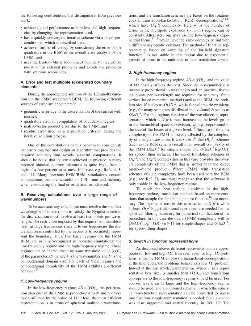
1. Comparison of algorithms

Figure 1 illustrates the present 3D Helmholtz FMM al-gorithm �on the right� and also compares it with that pro-posed in Ref. 17. These algorithms have in common theseparation of the high- and low-frequency regions where dif-ferent translation methods are used. It is seen that the presentalgorithm at high frequencies implements the idea used inthe algorithm17 for lower frequencies, while instead of con-version to the exponential form the spherical transform isused to convert the multipole expansion to the signaturefunction representation and back. The signature function rep-resentation is omnidirectional and, in contrast to the expo-nential forms, does not require additional data structures andmultiple representations �since translations for this represen-tation are different in each coordinate direction�. Also, thisapproach is valid for the values of p are necessary for thehigh-frequency region. However, despite the use of these ef-ficient techniques, the present algorithm has a formal trans-lational scaling O�p3� since in the high-frequency region forthe multipole-to-multipole S �S and local-to-local R �R opera-tors the spherical function representations are used.

2. Data structure

The version of the FMM used in this paper employs anoctree-based data structure, when the computational domainis enclosed into a cube of size D�D�D, which is assignedto level 0, and further the space is subdivided by the octree tothe level lmax. The algorithm works with cubes from level 2to lmax. For generation of the data structure, we use hierar-

S S

S

S

S

S

FS

F

RR

R

R

R

R

F R

F

Sp Sp-1

Sp-1Sp

F|F

F|F

S|R

S|S

S|S

S|S

R|R

R|R

R|R

S

S S E

R

RRE

Sp-1

S

FF

F

Sp

F|F+iF|F

S|S

R|R

E|E

S|E E|R

R

F F

F

F|F+f

F|F

high frequency

low frequency

Cheng et al (2006) Present

S E REE|E

S|E E|R

S|S

R|R

S|R

S S

S

S

S

S

FS

F

RR

R

R

R

R

F R

F

Sp Sp-1

Sp-1Sp

F|F

F|F

S|R

S|S

S|S

S|S

R|R

R|R

R|R

S

S S E

R

RRE

Sp-1

S

FF

F

Sp

F|F+iF|F

S|S

R|R

E|E

S|E E|R

R

F F

F

F|F+f

F|F

high frequency

low frequency

Cheng et al (2006) Present

S E REE|E

S|E E|R

S|S

R|R

S|R

FIG. 1. �Color online� Illustration comparing the wideband FMMs of Chenget al. �Ref. 17� and that presented in this paper for a problem in which theFMM octree has four levels and in which the high-low frequency switchthreshold occurs between levels 2 and 3. The left hand side for each algo-rithm shows the FMM upward pass, while the right hand side shows theFMM downward pass. Each box represents various steps for that level, suchas multipole expansion �S�, local expansion �R�, far-field signature functionsamples �F�, and exponential form for each coordinate direction �E�. The“glued” boxes mean that for a given box at that level the two types ofexpansions are constructed. S �S, R �R, S �R, E �E, and F �F denote translationoperators acting on the respective representations. Sp and Sp−1 denote for-ward and inverse spherical transform, S �E and E �R are the respective con-version operators. F �F+ i and F �F+ f mean that the translation is accompa-nied by use of an interpolation or filtering procedure.

chical box ordering based on the bit interleaving and pre-


compute lists of neighbors and children, which are storedand used as needed. The FMM used skips “empty” boxes atall levels.

3. Level-dependent truncation number

Each level is characterized by the size of the expansiondomain, which is the radius al of the circumsphere of theboxes at level l. Selection of the truncation number in thealgorithm is automated based on an expression of the formpl= p�kal ,� ,��, where � is the prescribed accuracy and � theseparation parameter �we used �=2 �see the justification inRef. 12��. A detailed discussion and theoretical error boundscan be found elsewhere �see e.g., Refs. 12 and 25�. Particu-larly, the following approximation combining low- and high-frequency asymptotics for monopole expansions can beutilized:12

plo = 1 −log ��1 − �−1�3/2

log �,

phi = ka +�3 log 1/��2/3

2�ka�1/3, �18�

p = �plo4 + phi

4 �1/4.

It is also shown in Ref. 12 that for the use of the rectangu-larly truncated translation operators the principal term of theerror can be evaluated based on this dependence. The nu-merical experiments show that the theoretical bound fre-quently overestimates the actual errors, so some correctionscan be also applied. The software developed here, in its au-tomatic setting, computes plo and phi and—if it happens thatp− phi� p*��, where p* is some number dictated by theoverall accuracy requirements—uses p= phi+ p*��; other-wise, Eq. �18� is used. In fact, we also had some bound forp*�� depending on ka to avoid blowout in computation offunctions at extremely low ka.

As previously mentioned, an automatic switch wasimplemented from the RCR-decomposition to the diagonalforms of the translation operators based on criterion kal

� �kD�*. The parameter �kD�* was based on the error bounds�18� and was selected for the level at which p− phi� p** �we

used p**=2�. This is dictated by the estimation of the thresh-

old at which the magnitude of the smallest truncated term inthe translation kernel �26� starts to grow exponentially �seeRef. 12�.

Figure 2 illustrates the dependence provided by Eq. �18�.We note that FMM with coarse accuracy like �=10−2 can beused for efficient preconditioning. We also can remark thatfunction representation via the multipole expansions anduse of the matrix-based translations �such as RCR-decomposition� is not the only choice, and in Refs. 14 and 17a method based on diagonalization of the translation opera-tors, different from Ref. 16, was developed. This method,however, requires some complication in data structure �de-composition to the x-, y-, and z-directional lists� and is effi-cient for moderate to large truncation numbers. As we men-tioned, the truncation numbers in the low-frequency region
can be reduced �plus the BEM itself has a limited accuracy

due to flat panel discretization�. In this case the efficiency ofthe matrix-based methods, such as the RCR-decomposition,has comparable or better efficiency. Indeed, function repre-sentations via the samples of the far-field signature functionsare at least two times larger, which results in larger memoryconsumption and reduction of efficiency of operations onlarger representing vectors.

4. Multipole expansions

Expansions over the singular �radiating� spherical basisfunctions Sn

m�r� in forms �15� and �16� can be applied torepresent the monopole source or respective integrals. Inthese formulas the singular and regular solutions of theHelmholtz equation are defined as

Snm�r� = hn�kr�Yn

m��,��, Rnm�r� = jn�kr�Yn

m��,�� ,

�19�n = 0,1,2, . . . , m = − n, . . . ,n ,

where in spherical coordinates r=r�sin � cos � , sin � sin � ,cos �� symbols hn�kr� and jn�kr� denote spherical Hankel�first kind� and Bessel functions, and Yn

m�� ,�� the sphericalharmonics,

Ynm��,�� = �− 1�m�2n + 1

4�

�n − �m��!�n + �m��!

Pn�m��cos ��eim�,

�20�n = 0,1,2, . . . , m = − n, . . . ,n ,

and Pn�m�� are the associated Legendre functions consistent

with that in Ref. 26, or Rodrigues’ formulas

Pnm�� = �− 1�m�1 − �2�m/2 dm

m Pn��, n � 0, m � 0,

FIG. 2. Dependences of the truncation number p on the dimensionless do-main size ka for different prescribed accuracies of the FMM � according toEq. �18� ��=2� �solid lines�. The dashed lines show the high-frequencyasymptotics phi�ka�. The circles mark the points of switch from functionrepresentation via multipole expansions to samples of the far-field signaturefunction and, respectively, the translation method used. The dash-dotted lineseparates the �ka , p� region into the domains where different function rep-resentations are used.

d�


Pn�� =1

2nn!

dn

d�n ��2 − 1�n, n � 0, �21�

where Pn�� are the Legendre polynomials.In the boundary integral formulation also normal deriva-

tives of Green’s function should be expanded �or integrals ofthese functions over the boundary elements�. These expan-sions can be obtained from expansions of the type of Eqs.�15� and �16� for the monopoles by applying appropriatelytruncated differential operators in the space of the expansioncoefficients,12 which are sparse matrices and so the cost ofdifferentiation is O�p2�. Indeed if �Cn

m� are the expansioncoefficients of some function F�r� over basis Sn

m�r�, while

�Cnm� are the expansion coefficients over the same basis of

function n ·�F�r� for unit normal n= �nx ,ny ,nz�, then

Cnm =

1

2��nx + iny��bn

mCn−1m+1 − bn+1

−m−1Cn+1m+1� + �nx − iny��bn

−mCn−1m−1

− bn+1m−1Cn+1

m−1�� + nz�anmCn+1

m − an−1m Cn−1

m �,

m = 0, � 1, � 2, . . . , n = �m�, �m� + 1, . . . , �22�

where anm and bn

m are the differentiation coefficients,

anm = an

−m =��n + 1 + m��n + 1 − m��2n + 1��2n + 3�

for n � �m� ,

anm = bn

m = 0 for n � �m� ,�23�

bnm =��n − m − 1��n − m�

�2n − 1��2n + 1�for 0 � m � n ,

bnm = −��n − m − 1��n − m�

�2n − 1��2n + 1�for − n � m � 0.

5. Translations

Translations of the expansions can be also thought of asapplications of matrices to the vectors of coefficients. Iftranslation occurs from level l to l� �l�= l−1 for the multipoleto multipole, or S �S-translation, l�= l for the multipole tolocal, or S �R-translation, and l�= l+1 for the local to local, orR �R-translation�, then pl�

2 translated coefficients relate to thepl

2 original coefficient via the pl�2

� pl2 matrix. Even for pre-

computed and stored matrices, this requires O�p4� opera-tions, which is unallowable cost for the translation if usingwith BEMs.12 Several methods to reduce this cost are wellknown. Particularly use of the RCR-decomposition of the�S �S��t�= �R �R��t� matrices

�R�R��t� = Rot−1�t/t��R�R��t�Rot�t/t� , �24�

where t is the translation vector, t= �t�, and Rot�t / t� is therotation matrix—which expresses coefficients in the rotatedreference frame, whose z-axis is collinear with t, while�R �R��t� is the coaxial translation operator �along axisz�—reduces the cost of application of all operators to O�p3�.As the geometry of the problem is specified, all these matri-ces can be precomputed for a cost of O�p3� operations using

13,12
recursions and can be stored. We note also that the rect-

angular truncation operators Rot�t / t� and Rot−1�t / t� act onthe vectors of length pl

2 and pl�2 , respectively, and produce

vectors of the same size, while �R �R��t� acts on a vector ofsize pl

2 and produces a vector of size pl�2 . Therefore, there is

no need for any interpolation or filtering as this is embeddedinto the decomposition. A similar decomposition is applied tothe �S �R��t� matrix for low frequencies, which provides anumerically stable low-frequency procedure �for levels cor-responding to kal� �kD�*�.

For levels with kal� �kD�*, we use the following de-composition of the translation matrix �S �R��t�:

�S�R��t� = Sp−1�s�t�Sp , �25�

where Sp can be thought of as a matrix of size Nl� pl2,

which performs transform of the expansion coefficients to Nl

samples of the far-field signature function �spherical trans-form�, �s�t� is a diagonal translation matrix of size Nl�Nl,and Sp−1 is a matrix of size pl

2�Nl, which provides a trans-form back to the space of the coefficients. The number ofsamples depends on the truncation number, and it is suffi-cient to use Nl= �2pl−1��4pl−3�, where the grid is a Carte-sian product of the 2pl−1 Gauss quadrature abscissas withrespect to the elevation angle −1��=cos ��1 and 4pl−3equispaced abscissas with respect to the azimuthal angle 0��2�. This grid also can be interpreted as a set of pointson the unit sphere �s j�. The entries of the diagonal matrix�s�t� are

� j j�t� = �n=0

2pl−2

in�2n + 1�hn�kt�Pn� s j · t

t, j = 1, . . . ,Nl,

�26�

which is a diagonal form of the translation operator.16 Thebandwidth of this function, 2pl−2, provides that decomposi-tion �25� of the pl

2� pl2 translation matrix �S �R��t� is exact.12

Note that for a given grid �which is the same for all transla-tions at level l�, the cost of computation of �s�t� for eachtranslation vector t is O�pl

3�. In the present implementation,all these entries are precomputed and stored, so no compu-tations of �s�t� are needed during the run part of the algo-rithm. The precomputation part may be sped up by employ-ing a data structure, which eliminates computations of � j j�t�for repeated entries s j · t / t and kt for all translations and, infact, allows a substantial reduction in the cost of the presentpart of the algorithm.

The operator Sp can be decomposed into the Legendretransform with respect to �=cos � followed by the Fouriertransform with respect to � �e.g., see Refs. 12, 17, and 27�. Ifperformed in a straightforward way, each of them requiresO�p3� operations. Despite the fact that there exist algorithmsfor fast Legendre transform and the fast Fourier transform�FFT� can be employed, which reduces the cost of applica-tion of operator Sp to O�p2 log p� or so, for moderate pstraightforward methods are much more efficient. Note thatthe major cost �about 90%� comes from the Fourier trans-
form, so if the FFT is applied efficiently, this speeds up the

procedure. Furthermore, the operator Sp−1 can be decom-posed into the inverse Fourier transform, diagonal matrix ofthe Legendre weights, and inverse Legendre transform. Thecost of this procedure is the same as that for the computationof the forward transform.

As mentioned earlier, since the same transforms Sp andSp−1 should be applied to all expansions at a given level, wecan make Eq. �25� more efficient than the RCR-decomposition by first applying the transform Sp to all boxexpansions at a given level, then performing all diagonaltranslations and consolidations, and, finally, applying trans-form Sp−1 to all boxes.

6. Evaluation of expansions

Finally we mention that for the computation of the BEMoperators L� and M�, the normal derivative of computedsums at the evaluation point should be taken. As the expan-sions are available for the sources outside the neighborhoodof the evaluation points, this can be performed by the appli-cation of the differentiation operator in the coefficient space�see Eq. �22��.

7. Simultaneous matrix-vector products

For an efficient iterative solution of Eq. �10�, the FMMcan be used to compute in one run the sum of four matrix-vector products together,

� + �� = �Ldense + Ldense� ��q� − �Mdense + Mdense� �� ,

�27�

for input vectors q and �. Also, if needed, results for theparts � and �� can be separated �e.g., for the application ofGreen’s identity alone for the computation of the potential atinternal domain points�. The dense parts of the matrices cor-respond to decomposition �14� and, in the case of use of asimple scheme �Eq. �17�� are the matrices with eliminateddiagonals.

V. COMPUTATION OF SINGULAR ELEMENTS

Despite the fact that there exist techniques for the com-putation of the integrals over the singular or nearly singularelements �e.g., with increasing number of nodes and elementpartitioning or using analytical or semianalytical formulas�,these methods can be costly, and below we propose a tech-nique for the approximation of such integrals, which is con-sistent with the use of the FMM and BEM. This technique issimilar to the “simple solution” technique used by some au-thors to compute the diagonal elements for the BEM forpotential problems and for elasticity,28 except that it is up-dated with the use of the FMM, and to the case of the Helm-holtz equation.

Let �x j� be a set of points sampling the surface, and Uj�

be a sphere of radius � centered at x j and Sj�=S�Uj

�. The
surface operators can be decomposed as

L�� = �Sj

��x�G�x,y�dS�x�

+ �S\Sj

��y,��x�G�x,y�dS�x� = Lj

�� + Lj�� ,

M�� = �Sj

��x�

�G�x,y��n�x�

dS�x�

+ �S\Sj

��y,��x�

�G�x,y��n�x�

dS�x� = Mj�� + M j�� .

�28�

Note that for small enough � we have the following approxi-mations of the integrals:

Lj�� jlj

��y�, Mj�� jmj

��y� , �29�

where functions lj��y� and mj

��y� are regular inside the do-main. Thus, they can be approximated by a set of some basisfunctions, which satisfy the same Helmholtz equation. Toconstruct such a set and approximation, consider Green’sidentity for a function, which is regular inside the finite do-main �internal problem�,

� = L� ��

�n − M�� , �30�

where =1 for points inside the domain, =1 /2 for pointson the boundary, and =0 for points outside the domain.Consider the following test functions:

��x� = eiks·x,

�31�

q�x� =��

�n�x� = n�x� · �eiks·x = ikn�x� · seiks·x, �s� = 1,

which represent plane waves propagating in any direction s.For these functions from Eqs. �28�–�30�, one obtains

mj��y� − ik�n j · s�lj

��y� = e−iks·xj�ikL��n · s�eiks·x�

− M�eiks·x� − �y�eiks·y� . �32�

Let s1 , . . . ,s4 be four different unit vectors provided thatfunctions eiks�·x, �=1, . . . ,4, are linearly independent. Thendenoting

� j��y� = eiks·xj�ikL��n · s��eiks�·x� − M�eiks�·x�

− �y�eiks�·y�, nj� = n j · s�, �33�

one obtains

mj��y� − iknj�lj

��y� = � j��y�, � = 1, . . . ,4. �34�

Obviously the surface operators L�� and M�� can be
similarly decomposed as

L�� = Lj�� + Lj��, M�� = Mj�

�� + M j�� ,

�35�Lj�

�� jlj��y�, Mj�

�� jmj��y� .

Note that these operators are employed only for points on theboundary, and the forms for internal and external problemsare either the same or related via a sign change. Thus one canuse Maue’s identity �8� for the internal problem. In this caseusing test functions �31�, Eqs. �32�–�34� can be modified asfollows:

mj��y� − iknj�lj�

��y� = � j�� y�, � = 1, . . . ,4,

�36�� j�� y� = e−iks·xj�ikL��n · s��eiks�·x� − M��eiks�·x�

− ��y�eiks�·y� ,

��y� = 12 ik�n�y� · s��, y � S .

Then for the chosen set of directions, solution will be pro-vided by the previous equations with mj

��y�, lj��y�, and

� j��y�, replaced with mj��y�, lj�

��y�, and � j�� y�, respectively.The small 4�2 linear systems for each �Eqs. �34� and

�36�� can be solved via least squares, and as noted above theFMM provides four simultaneous matrix-vector multiplica-tions, and so four matrix-vector products via the FMM ��=1, . . . ,4� are sufficient to get all diagonals.

A. Discretization

The above formulas obviously provide expressions forthe diagonal elements of matrices

Ljj = lj��x j�, Mjj = mj

��x j�, Ljj� = lj��x j� ,

�37�Mjj� = mj�

��x j�, j = 1, . . . ,N .

In fact, for the solution of the boundary integral equation,only quantities Ljj + Ljj� and Mjj + Mjj� are needed. So forgiven the storage can be reduced twice. Also combinationsLjj + Ljj� and Mjj + Mjj� can be computed instead using thesame method as described above.

VI. NUMERICAL EXPERIMENTS

The BEM/FMM was implemented in FORTRAN 95 andwas parallelized for symmetric multiprocessing architec-tures, such as modern multicore PCs, using OpenMP. Theresults reported below were obtained on a four core PC �IntelCore 2 Extreme QX6700 2.66 GHz processor with 2�4 Mbytes L2 Cache and 8 Gbytes random access memory�RAM�� running Windows XP-64. Parallelization requiresthe replication of data among threads and is controlled by thesize of the cache. In this implementation, to reduce the sizeof the stack only the sparse matrix computations and theS �R-translations using the RCR-decomposition �i.e., opera-tors employed for levels finer than the high-low-frequencyswitch level� were parallelized. Such a parallelization strat-egy was found to be efficient enough �overall parallelizationefficiency was about 80%–95%� and enabled computationsfor kD’s up to 500. For kD�200 more data can be placed on
the available stack, and a complete parallelization with effi-

ciency close to 100% was obtained. However, the resultsreported here use the partial parallelization to enable a uni-form comparison of the results obtained over a wide range ofkD’s.

A. Scattering from a single sphere

The example of an incident plane wave off a singlesphere is valuable for tests of the performance of the methodsince an analytical solution is available in this case. For theincident field �in�r�=eiks·r, where s is the unit vector collin-ear with the wave vector, the solution for the total �incidentplus scattered field� for impedance boundary conditions canbe found elsewhere, e.g., in Ref. 12,

��S�s�� =i

�ka�2 �n=0

�2n + 1�inPn�s · s��

hn��ka� + �i�/k�hn�ka�,� ��

�n+ i��

S= 0,

�38�

where a is the sphere radius, s� is a unit vector pointing tothe location of the evaluation surface point, and � is theboundary admittance, which is zero for sound-hard surfacesand infinity for sound-soft surfaces. Depending on this, onemay have for the scattered field a Neumann, Dirichlet, orRobin problem.

The following were varied in the simulations: k, discreti-zation, parameter in Eq. �10�, the boundary admittance,tolerance, and parameters controlling the FMM accuracy andperformance. A typical computational result is shown in Fig.3.

1. Preconditioning

The best preconditioners found were right precondition-ers that compute the solution of the system A� j =cj at the jthstep using unpreconditioned GMRES �inner loop� and lowaccuracy FMM with lower bounds for convergence of itera-tions. For example, if in the outer loop of the fGMRES theprescribed accuracy for the FMM solution was 10−4 �actualachieved accuracy was �10−6� and the iterative process wasterminated when the residual reaches 10−4, for the inner pre-conditioning loop we used FMM with prescribed accuracy of0.2 �actual accuracy was �5�10−3� and the iterative processwas terminated at a residual value of 0.45. The inner loopsolution was much faster than the outer loop, as it is stopped

FIG. 3. �Color online� Typical BEM computations of the scattering problem.The graph shows comparison between the analytical solution �38� and BEMsolution for the vicinity of the rear point of the sphere for ka=30.

after fewer iterations, and the matrix-vector product was sev-


eral times faster �lower truncation numbers�. The precondi-tioner reduced by an order of magnitude the number of itera-tions in the outer loop, more than compensating for theincreased cost of inner iterations. Beyond the benefit of im-proved time, this also has the benefit of reduced memory forlarge problems. This is because in the GMRES or fGMRESK vectors of length N must be stored, where K is the dimen-sionality of the Krylov subspace. The iterative process be-comes slower if K is restricted, and GMRES is restartedwhen K vectors have been stored. Hence it is preferable toachieve convergence in Niter�K iterations. In the case of theGMRES-based preconditioner, the storage memory is of or-der �K+K��N, where K� is the dimensionality of the Krylovsubspace for preconditioning. Since both K and K� are muchsmaller than the K required for unpreconditioned GMRES,the required memory for solution is reduced substantially.

Figure 4 shows the convergence of the unpreconditionedGMRES and the preconditioned fGMRES with the FMM-based preconditioner as described above. The computationswere made for a sound-hard sphere of radius a, whose sur-face was discretized by 101 402 vertices and 202 808 trian-gular elements for the relative wavenumber ka=50. The pre-conditioned iteration converges three times faster in terms ofthe time required. The matrix-vector product via the low ac-curacy FMM in preconditioning was approximately seventimes faster than that computed with higher accuracy in theouter loop �1.4 s versus 9.75 s�. The overall error of the ob-tained solution was slightly below 5�10−4 in the relativeL2-norm.

2. Spurious modes

The test case for the sphere is also good to illustrate theadvantage of the Burton–Miller formulation over the formu-lation based on Green’s identity. According to theory,20,29 theGreen’s identity formulation may result in convergence to asolution, which is the true solution plus a nonzero solution ofthe internal problem corresponding to zero boundary condi-tions at the given wavenumber. Such solutions are not physi-

1.E-04

1.E-03

1.E-02

1.E-01

1.E+00

0 20 40 60 80 100 120

Iteration #

Err

or

of

Resi

du

al

Unpreconditioned

Preconditioned

0

20

40

60

80

100

120

0 20 40 60 80 100 120

Iteration #

Com

puta

tion

alC

ost

Converged (10-4

)

Converged (10-4

)

Unpreconditioned

Preconditioned

1.E-04

1.E-03

1.E-02

1.E-01

1.E+00

0 20 40 60 80 100 120

Iteration #

Err

or

of

Resi

du

al

Unpreconditioned

Preconditioned

0

20

40

60

80

100

120

0 20 40 60 80 100 120

Iteration #

Com

puta

tion

alC

ost

Converged (10-4

)

Converged (10-4

)

Unpreconditioned

Preconditioned

FIG. 4. Left: The absolute error in the residual in the unpreconditionedGMRES �triangles� and in the preconditioned fGMRES �circles� as a func-tion of the number of iterations �outer loop for the fGMRES�. Right: therelative computational cost to achieve the same error in the residual forthese methods �1 cost unit=1 iteration using the unprecoditioned method�.Computations for sphere; ka=50 for mesh with 101 402 vertices and202 808 elements, and =6�10−4i.

cal since the solution of the external scattering problem is


unique, and, therefore, they manifest a deficiency of the nu-merical method based on the Green’s identity.

For a sphere any internal solution can be written in theform

�int�r� = �n=0

jn�kr� �m=−n

n

BnmYn

m��,�� , �39�

where �r ,� ,�� are the spherical coordinates of r and Bnm are

arbitrary constants. The set of zeros of the functions jn�ka�provides a discrete set of values of ka for which ��int�S=0,even though �int is not identically zero inside the sphere. Theminimum resonant k can be obtained from the first zero ofj0�ka�, which is ka=�. We conducted some numerical testswith Burton–Miller and Green’s formulations for a range ofka �0.01�ka�50� for different resonant values of ka.

Figure 5 provides an illustration for case ka=3� 9.424 778, which is the third zero of j0�ka�. When theBurton–Miller formulation is used with some with Im� ��0, a solution consistent with Eq. �38� is obtained, whilewhen computations are performed using Green’s formula awrong solution with the additional spurious modes isachieved. We checked that in this case the converged solu-tion can be well approximated ��=0� by

��S�s�� = B +i

�ka�2 �n=1

�2n + 1�inPn�s · s��

hn��ka�, �40�

where B is some complex constant depending on the initialguess in the iterative process. This shows that, in fact, thezero-order harmonic of the solution, corresponding to theresonating eigenfunction, failed to be determined correctly,which is the expected result. Note that such solutions appearwhen iterative methods are used, where degeneration of thematrix operator for some subspace does not affect conver-gence in the other subspaces. If the problem is solved di-rectly, the degeneracy or poor conditioning of the system

FIG. 5. Solutions of the plane wave scattering problem obtained using BEMwith the Burton–Miller and Green’s identity formulations and fGMRES it-erator for a sphere at resonance ka=9.424 778 �triangular mesh of 15 002vertices and 30 000 elements�. Analytical solution is shown by the circles.

matrix would result in a completely wrong solution.


In the nonresonant cases, the Green’s formulation pro-vided a good solution, while normally the number of itera-tions was observed to increase as ka comes closer to a reso-nance. For large ka �40 or more�, computations usingGreen’s identity become unstable, which is explainable bydensity of the zeros of jn�ka�. For the Burton–Miller formu-lation, the empirically found value of the parameter was

=i�

k, � � �0.01,1� . �41�

For the case above �=0.03 provides good results, while forka�1 the number of iterations increases compared to theGreen’s identity, and when there are certainly no resonances,Green’s identity can be recommended. Increase in this pa-rameter usually decreases the accuracy of computations sincemore weight is put on the hypersingular part of the integralequation, while decrease in the parameter for large ka leadsto an increase in the number of iterations. For ��0.01 theBurton–Miller integral equation shows the problems of spu-rious modes.

3. Performance

For the FMM, the characteristic scale is usually basedon the diagonal �maximum size� of the computational do-main, D, and kD is an important dimensionless parameter.Further, one can compute the maximum size of the boundaryelement, which for a triangular mesh is the maximum side ofthe triangle, d. This produces another dimensionless param-eter, kd. For a fixed body of surface area S�D2, the numberof elements in the mesh is of the order N�S /d2�D2 /d2. Aformal constraint for discretizations used for an accurate so-lution of the Helmholtz equation is d / a�1, where a

=2� /k is the acoustic wavelength. In practice this conditioncan be replaced with kd��, where � is some constant oforder 1, so there are not less than 2� /� mesh elements perwavelength. This number usually varies in range of 5–10.This shows that the total number of elements should be atleast N�D2 /d2� �kD�2 /�2=O��kD�2�.

Figure 6 shows the results of numerical experiments forscattering from a sound-hard sphere, where we fixed param-eter � 0.94 for kD�20, which provided at least six ele-ments per wavelength and increased the number of elementsproportionally to �kD�2 �the maximum case plotted corre-sponds to kD=500 where the mesh contains 1 500 002 ver-tices and 3 000 000 elements�. Additional data on some testsshowing the relative error in the L2-norm, �2, and peakmemory required for the problem solution for the currentimplementation are given in Table I. Note that in all cases therelative error in the L-norm was less or about 1%. For kD�3, which we characterize as very low-frequency regime,we used a constant mesh with 866 vertices and 1728 ele-ments. Also for this range was set to zero, while for othercases was computed using Eq. �41� with �=0.03. The timeand memory required for computations substantially dependon the accuracy of the FMM, tolerance for convergence, andsettings for the preconditioner. The prescribed FMM errorfor the outer loop was 10−4, which, in fact, provides accuracy

−6
about 10 in the L2-norm. This was found from the tests,

where the actual FMM error was computed by comparisonswith the straightforward �“exact”� method at 100 checkpoints. The prescribed accuracy for the preconditioner was4.5�10−2, which also substantially overestimates the actualaccuracy. Tolerance for convergence for the outer loop was10−4, while that for the inner loop was 0.45, where the num-ber of iterations was limited by 11. The memory requireddepends on the dimensionalities of the Krylov subspaces forthe outer and inner loops, which were set to 35 and 11,respectively, while the convergence for all cases was within20 outer iterations, so the memory, in fact, can be reduced.Additional acceleration can be obtained almost for all casesby the storage of the near-field data �matrix Asparse, Eq. �14��.However, based on the RAM �8 Gbytes� this works only forN�5�105. To show a scaling without jumps, such a storagewas not used, and the sparse matrix entries were recomputedeach time as the respective matrix-product was needed.

a. Computational complexity scaling. The total time re-quired for the solution of the problem is scaled approxi-mately as O��kD�2.4�, while the times for the matrix-vectormultiplication in the outer and in the inner iteration loops ofthe preconditioned fGMRES scale, respectively, asO��kD�2.2� and O��kD�2.04�. A standard least squares fit forthe data at kD�10 was used.

These results require some analysis and explanationsince the theoretical expectation of the matrix-vector com-plexity for the current version of the FMM is O��kD�3�.There are several different reasons that the algorithm isscaled better. First, we note that the complexity of the sparsematrix-vector product, which in a well-balanced algorithm

FIG. 6. Wall clock time and the number of iterations for solution of scat-tering problem from a sound-hard sphere in range 0.1�kD�500. Thecurves that fit the time to the data at high frequencies were obtained usingleast squares.

TABLE I. Error, memory, and FMM-BEM solution wall clock time for som

kD 0.0001 0.01 1 20N 866 866 866 2402 1�2 3.3�10−5 3.3�10−5 1.1�10−4 5.4�10−3 2.Memory, Mbyte 20 20 32 63Time, s 0.438 0.406 0.656 7.59


takes a substantial part of the computational time, is scaledas O�N�, i.e., as O��kD�2�. Second, for high-frequency com-putations a switch between the high-frequency and low-frequency representations always happens. As soon as thelow-frequency part is limited by condition kal� �kD�*,where �kD�* depends on the prescribed accuracy only, thecomputational cost for this part becomes proportional to thenumber of occupied boxes in the low-frequency regime. Thisnumber is O�Blmax

�, where Blmaxis the number of occupied

boxes at the finest level lmax, which for simple shapes isO�N�=O��kD�2�. Therefore, the low-frequency part for thefixed prescribed accuracy can be executed in O��kD�2� time.Therefore, all the O��kD�3� scaling comes only from thehigh-frequency part. However, here the most expensive partrelated to the S �R-translations is performed using the diago-nal forms with complexity O��kD�2�, while the asymptoticconstant related to the S �S- and R �R-translations and spheri-cal transform is relatively small. Profiling of the algorithmshows that sparse matrix-vector multiplication andS �R-translations in the low-frequency part contribute up to90% to the complexity in the range of kD’s studied. Addingall these facts together, we can see that the FMM for prob-lems solved is rather the O��kD�2� algorithm, and small ad-dition to power 2 is due to O��kD�3� operations with muchsmaller asymptotic constant.

According to the above discussion, the complexity of theFMM can be estimated as

Time = A�kD�3 + B�kD�2, �42�

where A and B are some constants. The least squares fit ofhigh-frequency data on the matrix-vector multiplication inthe outer loop with Eq. �42� is as good as fit O��kD�2.19�,shown in Fig. 6, and provides B /A=1.39�103. This number,indeed, is large, and it actually shows that only at kD�103

the high-frequency asymptotical behavior can be reached forthe prescribed accuracy of 10−4. For the low accuracy pre-conditioner used, this ratio becomes even smaller �B /A=1.75�103�, which justifies its applicability even for higherkD’s.

The overall algorithm scaling as O��kD�2.4� now is notsurprising since the factor O��kD�0.2� can be ascribed to the�slowly� increasing number of iterations. Indeed, Fig. 6shows that the number of iterations in the outer loop growsslowly.

b. Memory complexity scaling. Theoretically, thememory required to solve the problem should be scaled asO�N�=O��kD�2�. Due to different possibilities for memorymanagement and optimizations, plus realization of trade-offoption memory versus speed and limited resources, the ac-tual scaling can deviate from the theoretical one. Table I

t cases with a spherical scatterer with known analytical solution.

100 200 300 400 500104 6�104 2.4�105 5.4�105 9.6�105 1.5�106

10−4 4.1�10−4 5.34�10−4 3.6�10−4 4.92�10−4 3.2�10−3

461 1144 2861 3755 47486 327 1990 5150 10 400 19 100

e tes

50.5�

25�

26853.


shows that in the implementation used for this paper, thememory required grows slower than O��kD�2� in the rangestudied. Certainly, it should be scaled not less than O��kD�2�at larger kD since at least several vectors of size N should bestored. The table provides some data, which show that com-putation of a million size problem with kD�500 is reachableon desktop PCs or workstations.

c. Comparison with recent publications. As discussedpreviously two regimes can be recognized in FMM-BEMsimulations, the low and high-frequency regimes. Tables IIand III indicate some results from papers published in thepast few years. The data here should be compared with thosepresented in Table I where data for the present code aregiven. Looking first at the high-frequency regime, there ap-pear to be three relevant papers �Refs. 9, 10, and 17�. Refer-ence 17 only has a FMM matrix-vector product, and a de-tailed comparison of the present algorithm and the one ofthat paper was provided in Sec. IV. As mentioned previously,the size of the discretization N in a BEM simulation shouldbe at least O�kD�2, although more points may be necessary ifthe geometry is complex. In each case the comparison isquite favorable for the present code.

The results of the best performing FMM BEM solver10

which appeared during the time when this paper was underreview, is compared with the present work. In this paper theauthors provide data on test cases for scattering from asphere, so a comparison was possible. In this case a Robinproblem �2� with �=1 and �=−1 / �10−10i� was solved for asphere of radius a=20 �kD=435�. The incident field wasgenerated by a source located at �0,0 ,10a�. Unfortunatelythere were no data on the iteration process used, and the onlynotice was that the process converged to the residual 10−5.So the same parameters were used for the present test case.Further, a mesh containing 1 046 528 panels was used. Sincethis mesh was not available, a mesh of similar size that could

TABLE II. Results from some recent FMM and FMfrequency regime. The performance of the FMM andsuperior �see Tables I and IV�. Data not reported arvalues reported can be considered as those applying

Ref. kD N N / �kD�2 Me

10 435 1 046 528 5.53 489 126.64 98 304 6.13 149 126.64 49 152 3.06 7917 544 646 143 2.09 517 544 619 520 2.09 11

TABLE III. Results from some recent FMM and FMfrequency regime. The performance of the FMM andsuperior �see Table I�. The parameter N / �kD�2 reprrestrictions imposed by the frequency.

Ref. kD N N / �kD�2 Mem T

9 16 1536 6.13 48009 16 98 304 6.13 148714 0.9375 45 056 51 263 … 4114 0.9375 704 801 … 27 3.464 200 000 16 668 …


be generated was used. This mesh contained 1 130 988 tri-angles and 565 496 vertices. Another mesh tried contained2 096 688 panels and 1 048 346 vertices. In the cited paperGreen’s identity was used, while in the present study thecombined Eq. �12� with from Eq. �41� is used. An increasein � from the value of 0.03 used for the solution of theNeumann problem to a value of 1.2 improved convergencefor the Robin problem. The results are shown in Table IV.

It is seen that the present algorithm performed one orderof magnitude faster, while the memory consumption was ofthe same order. Of course, the present algorithm was paral-lelized and executed on a four core machine, compared to theone core serial implementation of the Multilevel Fast Multi-pole Algorithm. However, even assigning a perfect parallel-ization factor of 4, we see that the same problem can besolved several times faster. The speed-up of the present al-gorithm can be related to several issues, one of which is thepreconditioning and use of the combined equation instead ofGreen’s identity. For the largest case reported in Table IV,the present iteration took 23 outer loop iterations, for whichmatrix-vector multiplication took about 61 s/iteration, whilefor the inner loop, which was in any case limited by 11iterations, the matrix-vector product took about27 s/iteration.

As far as low-frequency computation comparisons areconcerned, comparisons were performed against Refs. 4, 7,and 9. Here again Table I shows that the present code hasperformance that is comparable or better. Here it is seen thatsome of the simulations reported in the literature have dis-cretizations that are much finer than what may have beenrequired by the problem.

B. More complex shapes

Many problems in acoustics require computations forsubstantially complex shapes, which include bioacoustics,

ccelerated BEM publications operating in the high-FMM-BEM reported in this paper is comparable oricated with a “–”; for the FMM only �Ref. 17� thee iteration of the solution procedure.

Error Time Iteration Remarks

�10−5 54 267 – Scattering0.03 24 325 59 Internal0.03 11 848 58 Internal10−3 672 n/a FMM only10−6 1832 n/a FMM only

ccelerated BEM publications operating in the low-FMM-BEM reported in this paper is comparable ors how overdiscretized the problem is vis-à-vis the

Iteration Time/Iteration Remarks

5 5.6 Internal room5 2.8 Internal room

452 92.2 Internal L-shape21 1.19 Internal L-shape

8000 … External scattering

M athe

e indto on

mory

00879.64911

M athe

esent

ime

2814962

5.1…


human hearing, sound propagation in dispersed media, en-gine acoustics, and room acoustics. Many such cases are re-ported in the literature: e.g., scattering off aircraft,17 offanimals,17 off engine blocks,7 and off many scatteringellipsoids.7 The present algorithm was tested on many suchcases to show that the iteration process is convergent forthese cases and that solutions can be obtained on bodies withthin and narrow appendages. Figure 7 provides an idea onthe sizes and geometries that were tested. Note that modelingof complex shapes requires surface discretizations, which aredetermined not only by the wavelength-based conditions ��2� but also by the requirements that the topology andsome shape features should be properly represented. Indeedeven for a solution of the Laplace equation �k=0�, theboundary element methods can use thousands and millionsof elements that just properly represent the geometry. Usu-ally the same mesh is used for multifrequency analysis, inwhich case the number of elements is fixed and selected tosatisfy criteria for the largest k required. In this case thenumber of elements per wavelength for small k can be large.Also, of course, discretization plays an important role in theaccuracy of computations. So if some problem with complexgeometry should be solved with high accuracy, then the num-ber of elements per wavelength can be again large enough.

The last geometry illustrated in Fig. 7 is similar to thecase studied in Ref. 7 for kD=3.464. Here the performanceand accuracy were studied for a range of kD from 0.35 to175 �ka=0.01–5, where a is the largest axis of an ellipsoid�.The surface of each ellipsoid was discretized with more than1000 vertices and 2000 elements to provide an acceptableaccuracy of the method even for low frequencies. The con-vergence for the Neumann, Dirichlet, and Robin problemswas very fast �just a few iterations� for small ka, where, asdiscussed above, the use of low-frequency FMM is neces-sary. The convergence was not affected by the increase in thenumber of nodes, although for accuracy better discretizations

TABLE IV. Comparison of solution times and memory at kD=435 reportedin Ref. 10 and the present study.

No. of elements N �unknowns� T �s� M �Gbyte�

10 1 046 528 1 046 528 54 267 4.8Present �case 1� 1 130 988 565 496 3 820 2.7Present �case 2� 2 096 688 1 048 346 7 762 2.8

FIG. 7. �Color online� Examples of test problems solved with the presentversion of the BEM: human head-torso, bunny models �7.85 and 25 kHzacoustic sources located inside the objects, kD=110 and 96, respectively�,
and plane wave scattering by 512 randomly oriented ellipsoids �kD=29�.

are preferred. As a test solution we used an analytical solu-tion when a source was placed inside one of the ellipsoids,and surface values and normal derivatives were computed ateach vertex location analytically. For larger discretizationsthat were used, we were able to achieve �1% relative errorsin strong norm �L� for the range of parameters used.

Figure 8 shows an absolute relative error at each vertex,

�i =��i

�BEM� − �i�an��

��i�an��

, i = 1, . . . ,Nvert, �43�

where �i�an� and �i

�BEM� are the analytical and BEM solutions,and ��i

�an�� is the modulus of the solution. The maximumerror here was max ��i�=1.58%, which is usually acceptablefor physics-based problems and engineering computations.

C. Computational challenges and drawbacks

Despite the fact that the present algorithm can run casesin a wide range of kD up to 500, the numerical stability forlarger kD is still a question. This mostly relates to the com-putation of matrix S �S- and R �R-translation operators athigher frequencies via the RCR-decomposition. Particularlywe should use different recursions for the computation ofentries of the rotation operators from those that were accept-able for lower truncation numbers than those described inour earlier paper13. Such recursions are available �see p. 336in Ref. 12� and stable if recursive backpropagation is used.An analysis shows that recursive computation of coaxialtranslation operators can be also unstable at larger frequen-cies, and this subject requires additional consideration, whichis beyond the present paper.

In terms of practical use of the algorithm, it is still aresearch question: how to improve preconditioning. For ex-ample, the current preconditioner worked well for the exter-nal Neumann problem in automatic settings, while the solu-tion of Robin or mixed problems showed a slow-down of theconvergence, and there was a need for intervention and tun-

FIG. 8. Solution �the upper curve� and error �the lower curve� in the bound-ary condition at each vertex for the case of the ellipsoids in Fig. 7.

ing of the � parameter and number of inner loop iterations


and accuracy to improve convergence. Further research onthe convergence of the iterative method is necessary.

VII. CONCLUSION

A version of the FMM accelerated BEM is presented,where a scalable FMM is used both for dense matrix-vectormultiplication and preconditioning. The equations solved arebased on the Burton–Miller formulation. The numerical re-sults show scaling consistent with the theory, which far out-performs conventional BEM in terms of memory and com-putational speed. Realization of a broadband FMM forefficient BEM requires different schemes for the treatment oflow- and high-frequency regions and switching from multi-pole to signature function representation. The tests of themethods for simple and complex shapes show that it can beused for an efficient solution of scattering and other acousti-cal problems encountered in practice for a wide range offrequencies.

ACKNOWLEDGMENTS

This work was partially supported by a Maryland Tech-nology Development Corporation grant in 2006 �at the Uni-versity of Maryland� and partially by Fantalgo, LLC. Wethank Dr. Vincent Cottoni and Dr. Phil Shorter of the ESIGroup U.S. R&D for a careful testing of the software ondifferent meshes before its inclusion in their VA-One prod-uct.

1L. Greengard, The Rapid Evaluation of Potential Fields in Particle Sys-tems �MIT, Cambridge, MA, 1988�.

2N. Nishimura, “Fast multipole accelerated boundary integral equationmethods,” Appl. Mech. Rev. 55, 299–324 �2002�.

3M. Fischer, “The fast multipole boundary element method and its appli-cation to structure-acoustic field interaction,” Ph.D. dissertation, Institut Afür Mechanik der Universität Stuttgart �2004�.

4M. Fischer, U. Gauger, and L. Gaul, “A multipole Galerkin boundaryelement method for acoustics,” Eng. Anal. Boundary Elem. 28, 155–162�2004�.

5T. Sakuma and Y. Yasuda, “Fast multipole boundary element method forlarge-scale steady-state sound field analysis, Part I: Setup and validation,”Acust. Acta Acust. 88, 513–525 �2002�.

6S. Schneider, “Application of fast methods for acoustic scattering andradiation problems,” J. Comput. Acoust. 11, 387–401 �2003�.

7L. Shen and Y. J. Liu, “An adaptive fast multipole boundary elementmethod for three-dimensional acoustic wave problems based on theBurton–Miller formulation,” Comput. Mech. 40, 461–472 �2007�.

8Y. Yasuda and T. Sakuma, “Fast multipole boundary element method forlarge-scale steady-state sound field analysis, Part II: Examination of nu-merical items,” Acust. Acta Acust. 89, 28–38 �2003�.


9Y. Yasuda and T. Sakuma, “An effective setting of hierarchical cell struc-ture for the fast multipole boundary element method,” J. Comput. Acoust.13, 47–70 �2005�.

10M. S. Tong, W. C. Chew, and M. J. White, “Multilevel fast multipolealgorithm for acoustic wave scattering by truncated ground with trenches,”J. Acoust. Soc. Am. 123, 2513–2521 �2008�.

11B. Chandrasekhar and S. M. Rao, “Acoustic scattering from rigid bodiesof arbitrary shape—double layer formulation,” J. Acoust. Soc. Am. 115,1926–1933 �2004�.

12N. A. Gumerov and R. Duraiswami, Fast Multipole Methods for the Helm-holtz Equation in Three Dimensions �Elsevier, Oxford, UK, 2004�.

13N. A. Gumerov and R. Duraiswami, “Recursions for the computation ofmultipole translation and rotation coefficients for the 3-D Helmholtz equa-tion,” SIAM J. Sci. Comput. �USA� 25, 1344–1381 �2003�.

14E. Darve and P. Havé, “Efficient fast multipole method for low-frequencyscattering,” J. Comput. Phys. 197, 341–363 �2004�.

15L. Greengrard, J. Huang, V. Rokhlin, and S. Wandzura, “Accelerating fastmultipole methods for the Helmholtz equation at low frequencies,” IEEEComput. Sci. Eng. 5, 32–38 �1998�.

16V. Rokhlin, “Diagonal forms of translation operators for the Helmholtzequation in three dimensions,” Appl. Comput. Harmon. Anal. 1, 82–93�1993�.

17H. Cheng, W. Y. Crutchfield, Z. Gimbutas, L. F. Greengard, J. F. Ethridge,J. Huang, V. Rokhlin, N. Yarvin, and J. Zhao, “A wideband fast multipolemethod for the Helmholtz equation in three dimensions,” J. Comput. Phys.216, 300–325 �2006�.

18Fast and Efficient Algorithms in Computational Electromagnetics, editedby W. C. Chew, J. M. Jin, E. Michelssen, and J. Song �Artech House,Boston, 2001�.

19Y. Saad, “A flexible inner-outer preconditioned GMRES algorithm,”SIAM J. Sci. Comput. �USA� 14, 461–469 �1993�.

20A. J. Burton and G. F. Miller, “The application of the integral equationmethods to the numerical solution of some exterior boundary-value prob-lems,” Proc. R. Soc. London, Ser. A 323, 201–210 �1971�.

21L. H. Chen and J. Zhou, Boundary Element Methods �Academic, NewYork, 1992�.

22S. Kirkup, “The boundary element method in acoustics,” http://www.boundary-element-method.com/acoustics/index.htm �Last viewedDecember 30, 2007�.

23Y. Saad and M. H. Schultz, “GMRES: A generalized minimal residualalgorithm for solving nonsymmetric linear systems,” SIAM �Soc. Ind.Appl. Math.� J. Sci. Stat. Comput. 7, 856–869 �1986�.

24N. A. Gumerov and R. Duraiswami, “Computation of scattering fromclusters of spheres using the fast multiple method,” J. Acoust. Soc. Am.117, 1744–1761 �2005�.

25E. Darve, “The fast multipole method �I�: Error analysis and asymptoticcomplexity,” SIAM �Soc. Ind. Appl. Math.� J. Numer. Anal. 38, 98–128�2000�.

26M. Abramowitz and I. A. Stegun, Handbook of Mathematical Functions�National Bureau of Standards, Washington, DC, 1964�.

27J. R. Driscoll and D. M. Healy, Jr., “Computing Fourier transforms andconvolutions on the 2-sphere,” Adv. Appl. Math. 15, 202–250 �1994�.

28E. Lutz, A. R. Ingraffea, and L. J. Gray, “Use of ‘simple solutions’ forboundary integral equation methods in elasticity and fracture analysis,”Int. J. Numer. Methods Eng. 35, 1737–1751 �1992�.

29D. Colton and R. Kress, Inverse Acoustic and Electromagnetic ScatteringTheory �Springer-Verlag, Berlin, 1998�.


a broadband fast multipole accelerated boundary element method …ramani/pubs/gumerovduraiswa… ·...

Documents