978-0-7844-1329-6.003

1

Some Recent and Emerging Topics on Seismic Wave Methods for Geotechnical Site Characterization

Dennis R. Hiltunen,1 Khiem T. Tran,2 and Pengxiang Jiang3

1Professor, University of Florida, Department of Civil and Coastal Engineering, 365 Weil Hall, P. O. Box 116580, Gainesville, FL 32611, E-mail: [email protected] 2Assistant Professor, Clarkson University, Department of Civil and Environmental Engineering, 234 Rowley Laboratories, Potsdam, NY 13699-5710, E-mail: [email protected] 3Graduate Research Assistant, University of Florida, Department of Civil and Coastal Engineering, 365 Weil Hall, P. O. Box 116580, Gainesville, FL 32611, E-mail: [email protected] ABSTRACT

New developments in surface-based seismic wave methods are described around three significant themes: 1) array signal processing, 2) numerical methods for solving the equations of wave propagation, and 3) global optimization methods for solving the inverse problem. These themes are illustrated via examples from surface wave, refraction-based travel time, and full waveform inversion techniques. Based on concepts from array signal processing, inversion of the combined dispersion curve from a non-uniform active-source surface wave array and a 2D passive-source array yielded a significantly deeper shear wave velocity profile for a site in Florida than produced using dispersion data from a sledgehammer source uniform array and ReMi. A new technique is presented to invert refraction-type first-arrival times using the multistencils fast marching method finite-difference solution of the Eikonal equation and simulated annealing global optimization. A comparison of inversion results utilizing the new technique to analyze data collected simultaneously within a borehole and along the ground surface against inversion results developed using just the surface data suggests that significant additional resolution of inverted profiles at depth are obtained, and uncertainties are significantly reduced with the addition of a borehole. Lastly, techniques are presented to invert full waveforms using two global optimization methods, a genetic algorithm and simulated annealing. The inversion scheme is based on a finite-difference solution of the 2D elastic wave equation in the time-distance domain. It is demonstrated that these inversion techniques are capable of characterizing both low- and high-velocity layers in laterally inhomogeneous profiles, and that full waveform inversion is computationally practical. INTRODUCTION

Engineering geophysical techniques enable “seeing” between instruments placed in boreholes, or from instruments placed entirely along the ground surface. Coupled with tomographic algorithms, a two-dimensional slice or a three-dimensional volume of the subsurface under study can be produced. Borehole geophysical methods typically provide the best accuracy and resolution, while surface-based techniques are typically more economical to implement, but can suffer from depth of penetration and resolution problems.

Measured wavefields carry substantial information about characteristics of media they propagate in, and wave evaluation techniques use this information to infer important properties.

53Geo-Congress 2014 Keynote Lectures, GSP 235 © ASCE 2014

2

For example, there are many seismic wave based techniques that are routinely used for shallow subsurface investigation, such as techniques using wave velocity dispersion, including spectral analysis of surface waves (SASW) (Nazarian 1984), multi-channel analysis of surface waves (MASW; Park et al., 1999), refraction microtremor (ReMi) (Louie 2001), and passive-source frequency-wavenumber (f-k), and techniques using travel times, including conventional seismic refraction and seismic refraction tomography. Surface wave and refraction techniques make use of only a portion of the complete wavefield, the normal modes of surface wave propagation and the first-arrival travel times, respectively. Alternatively, the emerging technique of full waveform inversion (FWI) (Plessix 2008 and Vireux and Operto 2009) offers the potential to produce more detailed resolution of the subsurface by extracting information contained in the complete waveforms. However, FWI is computationally intensive, as it requires a complete solution of the governing wave equation.

The aim of the paper is to review recent improvements and advancements in surface-based seismic wave methods. In cases where they provide meaningful characterization information, surface methods often offer significant economic advantages over borehole methods. As a consequence, surface methods are a primary focus of current research activity. The new developments reviewed herein are built around three significant themes: 1) array signal processing, 2) numerical methods for solving the equations of wave propagation, and 3) global optimization methods for solving the inverse problem. These themes are illustrated via examples from surface wave, refraction-based travel time, and full waveform inversion techniques. SURFACE WAVES

Based on concepts from array signal processing, techniques have emerged over the past

decade that aim to further improve the accuracy and resolution of surface wavefield characterization, particularly at low frequencies which serves to increase the depth of characterization. Using a small vibration shaker, a linear array of non-uniformly spaced geophones, and array-based cylindrical beamformer two-dimensional wavefield transformations, Hebler (2001) demonstrated significantly improved determination of the Rayleigh wave dispersion relationship. Rosenblad and Li (2009) utilized these concepts with a large vibration shaker to successfully characterize test sites in the Mississippi Embayment to several hundred meters in depth. A number of research studies have recently utilized arrays of transducers arranged two-dimensionally (e.g., circle, triangle, L-shape) to collect wavefield signals from passive vibration sources. Since the location of a passive source is typically unknown, a 2D array is able to resolve both the speed and the direction of wave propagation, which provides a more accurate determination of wavefield velocity than can typically be accomplished with a linear array. The study of Rosenblad and Li (2009), for example, provides several comparisons between 1D and 2D arrays, and demonstrates the limitations that may be encountered with 1D arrays, particularly at the lowest frequencies. Thus, array-based signal processing, non-uniform array active techniques, and 2D passive arrays appear to provide improved techniques for deeper and more accurate characterization of geotechnical engineering sites.

A demonstration of the capabilities of these new techniques is presented using data collected from a field site in Florida that has been previously characterized with several other geophysical and geotechnical methodologies. The data were collected at a Florida Department of Transportation (FDOT) storm water runoff retention basin in Alachua County off of state road


3

26, Newberry, Florida. The test site generally consists of approximately 6.1 m (20 ft) of an upper layer of mixed sand and clay soils, followed by limestone bedrock.

Conventional active-source MASW tests were conducted with 31 4.5-Hz geophone receivers oriented vertically at a spacing of 0.61 m (2 ft) with the total receiver spread of 18.3 m (60 ft), and a sledgehammer source was located 9.1 m (30 ft) away from the first receiver. Conventional passive-source multi-channel (ReMi) tests were conducted with 32 4.5-Hz geophone receivers oriented vertically and deployed at an inter-spacing of 3.0 m (10 ft) and spanning a distance of 94.5 m (310 ft). In addition, ReMi tests were also conducted along the same line using 16 1-Hz geophones oriented vertically and spaced first at 3.0-m (10-ft) intervals and then at 6.1-m (20-ft) intervals.

To investigate the proposed new techniques, array-based active tests were collected with a non-uniform linear array of 16 1-Hz geophones oriented vertically and driven with an APS Dynamics 400 portable shaker. The non-uniform array consisted of geophones located at 2.4, 3.0, 3.6, 4.6, 5.7, 6.7, 8.5, 10.4, 12.8, 15.2, 18.3, 21.3, 24.4, 29.0, 33.5, and 39.0 m (8, 10, 12, 15, 18, 22, 28, 34, 42, 50, 60, 70, 80, 95, 110, and 128 ft) from the fixed shaker position. Passive-source multi-channel tests were conducted with two circular (2D) arrays: a 30-m (100-ft) diameter array with 31 4.5-Hz geophones oriented vertically and equally-spaced around the circumference, and a 60-m (200-ft) diameter array with 16 1-Hz geophones oriented vertically and equally-spaced around the circumference.

Figure 1 presents a comparison of the power spectra results (2D and 3D) for the uniformly-spaced MASW-style data and the non-uniformly-spaced alternative procedure. The spectra were determined via the cylindrical beamformer technique (Zwicki 1999, Tran and Hiltunen 2008). The presented results are so-called dispersion images based on multi-channel analysis of all types of seismic waves propagating along the surface. The dispersion images are a form of three-dimensional power spectrum, in which the surface wave phase velocity versus frequency (dispersion) of the propagating waves is displayed on the horizontal axes, and the energy present at each velocity-frequency pair is displayed via a color coding, with the cool colors of low energy, and the hot colors of high energy. A concentration of high energy over a narrow band represents a normal mode of wave propagation, and the velocity-frequency pairs along the peak of the narrow band is typically referred to as the dispersion curve in surface wave testing. A dispersion curve is a relationship showing how surface wave phase velocity of a layered material changes with frequency (or wavelength). The MASW-style results in Figures 1a and 1b suggest that a fundamental mode of the Rayleigh wave can be reliably extracted for frequencies from about 10 to 85 Hz. However, the fundamental mode is discontinuous and higher modes of wave propagation are observed in the spectra. For the non-uniform array results in Figures 1c and 1d, the fundamental mode of the Rayleigh wave is smoother, and a narrow band of energy in 2D and a sharp ridge in 3D is observed over a wide range of frequencies. A fundamental mode can be reliably extracted for frequencies from about 4 to 100 Hz. The better performance at low frequencies is particularly noteworthy.

Two sets of 2D passive array data were collected and examined herein as detailed above: a 30-m (100-ft) diameter circular array and a 60-m (200-ft) diameter circular array. Each data set consisted of 20 32-second records. Three signal processing algorithms well described by Zwicki (1999) were used to produce dispersion curve images from the 2D array data, frequency domain beamformer (FDBF), multiple signal classification (MUSIC), and minimum variance distortionless look (MVDL).


4

For both 2D arrays, FDBF and MUSIC produced similar dispersion images, whereas the MVDL did not produce useful results. The poor performance of MVDL was similar to that reported by both Zwicki (1999) and Li (2008). From the dispersion curve images from the FDBF

(a) Z line, 2-ft uniform, 4.5 Hz (b) Z line, 2-ft uniform, 4.5 Hz

(c) K line, nonuniform, 1 Hz (d) K line, nonuniform, 1 Hz

Figure 1. Phase velocity and normalized amplitude vs. frequency spectra by cylindrical beamformer for two active-source arrays at Newberry Test Site.

0 0.1 0.2 0.3 0.4 0.5 0.6 0.7 0.8 0.9


5

for both arrays, it was noted that the 30-m (100-ft) diameter array yielded a dispersion image from about 9 to 20 Hz, while the 60-m (200-ft) diameter array further extended the dispersion image down to about 4 Hz. Within the range of overlap between 9 and 14 Hz, the two images are similar, though the smaller array results show slightly higher phase velocities. Yoon (2005) has shown that the poorer wavenumber resolution from the smaller array will tend to overestimate phase velocity in a multi-energy environment.

Also of interest, from the dispersion curve results for both the ReMi and 2D array data it was observed that both produce reliable dispersion data for frequencies up to nearly 25 Hz. The dispersion data from the ReMi and 2D arrays were in good agreement for frequencies from about 25 Hz on the high end and down to about 7 or 8 Hz on the low end. For frequencies below about 7 or 8 Hz, the phase velocity estimates from ReMi are lower than from the 2D array.

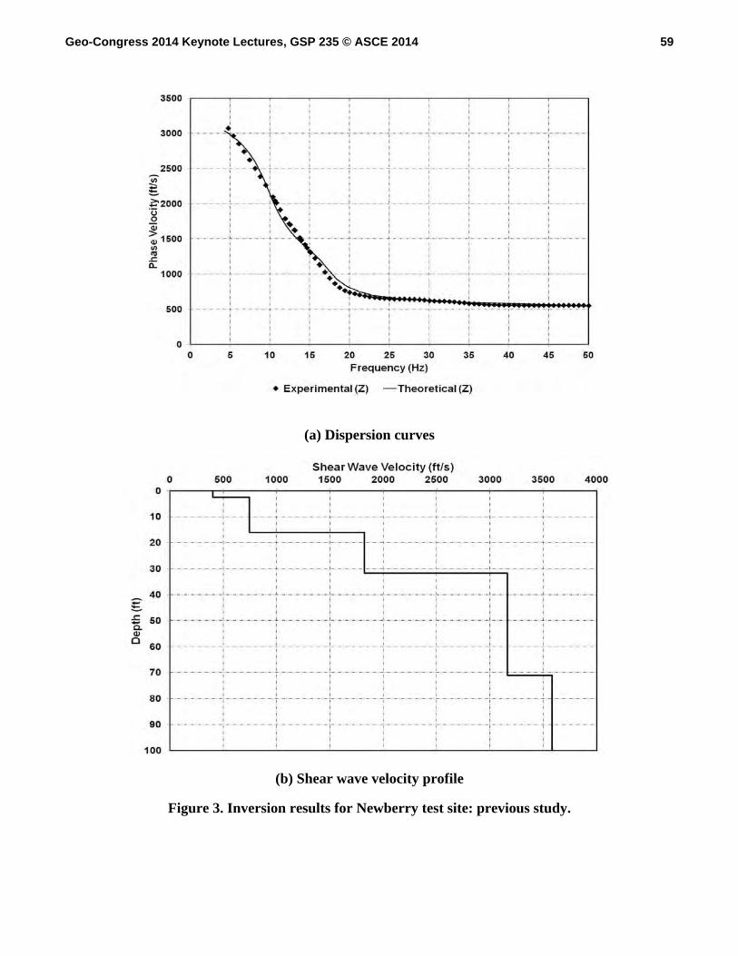
As a final step in the analysis of the Newberry site data, inversion of the dispersion data for the variation of shear wave velocity with depth was conducted. To begin, the active and passive dispersion data were combined and smoothened to produce the dispersion data shown in Figure 2a. Next, an inversion routine available in the SeisOpt ReMi commercial software produced a shear wave velocity profile from the combined data. The resulting fit of the dispersion data was excellent as shown in Figure 2a, and the shear wave velocity profile for the site is shown in Figure 2b. For comparison, Figure 3 presents dispersion data and an inverted shear wave velocity profile reported in an earlier study by Tran and Hiltunen (2008). The dispersion data for this previous study were determined by combining the uniform-array MASW-style active data with ReMi data, and the shear wave velocity profile was determined via the same inversion routine available in the SeisOpt ReMi software mentioned above.

It is noted that the new techniques produced a dispersion curve down to a lowest frequency of about 4 Hz, while the previous study produced dispersion data down to about 5 Hz. This comparison provides a remarkable testimony to how important this seemingly small difference of only 1 Hz can be at these low frequencies. Inversion of the dispersion data to 5 Hz produced a shear wave velocity profile to a depth of about 21 m (70 ft), while inversion of the dispersion data to 4 Hz produced a profile to a depth of about 145 m (475 ft), a difference of nearly seven times. The improved resolution of low frequencies by the new techniques dramatically increased the depth of characterization and provides a good example of the added benefit of recent developments in array signal processing techniques. SEISMIC REFRACTION TOMOGRAPHY

Seismic refraction tomography techniques have provided a significant new geophysical tool that have been made possible by: 1) the coupling of efficient numerical methodologies to solve the relevant equations of wave propagation (i.e., the forward model) with modern computers, and 2) the utilization of optimization techniques to efficiently search the parameter space for plausible models to describe the subsurface (i.e., the inversion routine).

Several initial studies (Carpenter et al. 2003 and Sheehan et al. 2005) indicated that refraction tomography performs well in many situations where traditional refraction techniques fail, such as velocity structures with both lateral and vertical velocity gradients. Hiltunen et al. (2007) mapped the limestone bedrock surface along several survey lines using both intrusive and geophysical techniques. Analyses of the site investigation data revealed a highly erratic limestone bedrock surface, which is common in karst terrain. Analysis of seismic refraction data demonstrated that commercially-available refraction tomography software systems are able


6

(a) Dispersion curves

(b) Shear wave velocity profile

Figure 2. Inversion results for Newberry test site: new techniques.


7

(a) Dispersion curves

(b) Shear wave velocity profile

Figure 3. Inversion results for Newberry test site: previous study.


8

to reveal the undulating bedrock surface. Hiltunen and Cramer (2008) collected seismic refraction tomography field data on several bridge foundation sites in Pennsylvania, in close proximity to geotechnical boring locations. From these data it appears that seismic wave tomograms can characterize the soil/rock interface, and that it is possible to predict expected design pile lengths based upon a measured P-wave velocity tomogram. Powell and Whiteley (2008) and Whiteley (2012) have also demonstrated the significant additional benefits that such images can provide during geotechnical site investigation studies. Finally, Zelt et al. (2013) presented a blind test of inversion and tomographic refraction analysis methods using a synthetic dataset. Fourteen estimated models were determined by ten participants using eight different inversion algorithms. The estimated models were generally consistent in terms of their large-scale features, demonstrating the robustness of refraction data inversion and the eight algorithms.

In the following, two new developments are presented that extend the capabilities of first-arrival travel time refraction tomography utilizing recent advancements in wave propagation modeling and inversion. Ground Surface. First, Tran and Hiltunen (2011) presented a new technique to invert first-arrival times using simulated annealing. The scheme is based on an extremely fast finite-difference solution of the Eikonal equation to forward compute the first-arrival time through the velocity models by the multistencils fast marching method. The core of the simulated annealing inversion, the Metropolis sampler, is applied in cascade with respect to shots to significantly reduce computer time. In addition, simulated annealing provides a suite of final models clustering around the global solution and having comparable least-squared error to allow determining uncertainties associated with inversion results.

Two main approaches that have been routinely used to calculate first-arrival times are the shortest path method (SPM) and the Eikonal equation solution. SPM originated in network theory (Dijkstra 1959) and was applied by Nakanishi and Yamaguchi (1986) and Moser (1991) to seismic ray tracing. The main advantage of SPM are its simplicity and capacity for simultaneous calculation of both the first arrival time and the associated ray path, but it takes more time for calculation and is not very efficient to use for the global optimization methods. The Eikonal equation has been solved by many authors, including Vidale (1988), Van Trier and Symes (1991), Nichols (1996), Sethian (1996 and 1999), Kim (1999), Chopp (2001), Hassouna and Farag (2007). Among these methods, the fast marching method (FMM) is typically considered the fastest and most stable and consistent method for solution of the Eikonal equation. It was first presented by Sethian (1996) and has been improved by other authors. In this study, the improved version of FMM by Hassouna and Farag (2007), the so called multistencils fast marching (MSFM), was utilized to compute first-arrival times for forward modeling. MSFM computes the solution at each point by solving the Eikonal equation along several stencils, and then picks the solution that satisfies the upwind condition.

Sen and Stoffa (1991, 1995), Pullammanappallil and Louie (1994), and Sharma and Kaikkonen (1998) have inverted various geophysical data sets with global inversion techniques such as simulated annealing, genetic algorithms, and other importance sampling approaches. Global inversion techniques attempt to find the global minimum of the misfit function by searching over a large parameter space. Most of the global inversion techniques are stochastic and use more global information to update the current position in an attempt to converge to the global minimum, which is important in cases where the model-data relationship is highly nonlinear and produces multimodal misfit functions (Sambridge and Mosegaard 2002).


9

Simulated annealing provides a suite of final models clustering around the global solution and having comparable least-squared error. This allows for determination of an inversion result by averaging all of these comparable models to mitigate the influence of noise and the non-uniqueness of the inversion solutions. On the other hand, a genetic algorithm is typically faster than simulated annealing. The most important objective of global inversion techniques is to avoid being trapped in local minima, and thus to allow final inversion results to be independent of the initial model. However, these global techniques can require significant computer time, especially if the model contains a large number of model parameters. This disadvantage is reduced herein by using an extremely fast forwarding model solution, and by sampling in cascade with respect to shot position. First-arrival time inversions usually require many shots to obtain a high-resolution profile and each shot needs a forwarding model solution. Meanwhile, global optimization methods sample over a large number of trial models, and only accept a small part of them. Using an acceptance rule in cascade, forwarding model solutions for only a few shots are often required to reject the biased models. To assess the capabilities of this new inversion technique, Tran and Hiltunen (2011) utilized both synthetic and real experimental data sets generated and collected along the ground surface. The inversion results show that this technique successfully maps 2-D velocity profiles with high variation.

First, the technique was tested on three synthetic models with high lateral variation and previously studied by Sheehan et al. (2005). The models included a notch (model 1), a stair step (model 2), and broad epikarst (model 3). For all three models, 25 shots into 48 geophones were used to create synthetic first-arrival times. The geophone spacing was 1 m for models 1 and 2, and 2 m for model 3. For all models, the 25 shots were within the geophone spread and the shot spacing was twice the geophone spacing. With this arrangement, the number of shots, number of geophones, and geophone spacing were the same as those used in Sheehan et al. (2005). By way of example, the results from model 3 are shown in Figure 4.

A primary feature of refraction tomography is delineation of both vertical and horizontal changes in seismic wave velocity. It is observed that the inverted model (Figure 4b) is an excellent recovery of the true model (Figure 4a). Both velocities and interfaces between layers are very well inverted. However, it is also observed that the inverted model is not identical to the true model. Most notably, as discussed by Sheehan et al. (2005) and others, refraction tomography will always model a sharp contrast in velocity with a gradient in velocity (this is usually a result of some method of smoothing of the velocity model such). This reality largely accounts for the differences in the two models. In addition, refraction tomography is not able to characterize zones of material outside of the ray coverage. Here is where the uncertainty results provided by the simulated annealing global optimization technique (Figure 4c) are helpful. The uncertainty is low in zones with good ray coverage, such as zones near the surface, and high in zones with poor ray coverage, such as zones near the bottom corners of the medium. In zones of high uncertainty, the inversion routine simply reports the velocity as the average value from all values randomly and uniformly withdrawn between the minimum and maximum velocity constraints selected by the user. Otherwise, in the zones of low uncertainty, the inverted velocity is independent of the constraints, and thus more reliable. From this and other synthetic model results, it appears that the delineation between low and high uncertainty is reasonably established at a COV value of approximately 20%. To test the new inversion algorithm on experimental data, Tran and Hiltunen (2011) also analyzed data from 12 seismic refraction tests collected in a study documented by Hiltunen et al. (2007). Each 36.6-m long refraction test was conducted with 4.5 Hz vertical geophones spaced


10

Figure 4. Synthetic model 3: a) true model, b) inverted model, and c) uncertainty associated with the inverted model. equally at 0.61 m, for a total of 61 measurements. Seismic energy was created by vertically striking a metal ground plate with an 89 N sledgehammer, thus producing compression wave (P-wave) first arrivals. Shot locations were spaced at 3.0-m intervals along the 36.6-m line and starting at 0 m, for a total of 13 shots. By way of example, data from gridline A is chosen to present herein because these data displayed the most variable condition along the line. Cone penetration tests (CPT), geotechnical borings, and standard penetration tests (SPT) were also conducted on gridline A for partially verifying the inverted P-wave tomograms.

Figures 5a and 6a present two-dimensional compression (P) wave refraction tomograms determined from test data collected along the surface. These tomograms indicate that the P-wave velocity at this site generally increases with depth, and that the specific pattern of increase depends on lateral location across the site. Figures. 5b and 6b show the uncertainties associated with the inverted P-wave profiles. Again, the uncertainty is consistent with expectations: low uncertainty in zones with good ray coverage (zones near the surface), and high uncertainty in zones with poor ray coverage (zones near the bottom corners of the medium). With the confidence gained from running synthetic models, the depth of investigation is about 10 m at the middle of the model where the COV from surface to that depth is less than 20 percent.

Following refraction data collection and analysis, invasive ground proving information was collected at the site to provide partial verification of the refraction test result interpretations, including four CPT soundings along line A at the following horizontal stations: 19.8, 39.6, 44.2, and 65.5 m. The length of each CPT run is shown atop the tomograms in Figures 5a and 6a. These results are compared with the refraction tomograms as follows:

0 10 20 30 40 50 60 70 80 90 100

Distance (m)

-15

-10

-5

0

Dep

th (

m)

0 10 20 30 40 50 60 70 80 90 100-15

-10

-5

0

Vel

ocity

(m

/s)

Coe

ffic

ien

t of V

aria

tion

(%)

a)

c)

b)

1000 m/s

3000 m/s0 10 20 30 40 50 60 70 80 90 100

Distance (m)

-15

-10

-5

0

Dep

th (

m)

1000

1500

2000

2500

3000

3500

4000

0 10 20 30 40 50 60 70 80 90 100

Distance (m)

-15

-10

-5

0

De

pth

(m)

0

10

20

30

40

50

60

1000 m/s

2000 m/s

4000 m/s


11

Figure 5. Inversion result for the real data A_0-36.6: a) Inverted model, and b) uncertainty associated with the inverted model. Figure 6. Inversion result for the real data A_36.6-73.2: a) Inverted model, and b) uncertainty associated with the inverted model.

P_w

ave

vel

ocity

(m

/s)

Coe

ffici

ent o

f V

aria

tion

(%)

a)

b)

0 5 10 15 20 25 30 35

Distance (m)

-10

-8

-6

-4

-2

0

Dept

h (m

)

0

2

4

6

8

10

12

14

16

18

20

22

24

26

A-19.8

0 5 10 15 20 25 30 35

Distance (m)

-10

-8

-6

-4

-2

0

Dep

th (m

)

0 5 10 15 20 25 30 35

-10

-8

-6

-4

-2

0

300

500

700

900

1100

1300

1500

1700

1900

2100

2300

P_w

ave

velo

city

(m

/s)

Coef

ficie

nt o

f V

aria

tion (%

)

40 45 50 55 60 65 70

Distance (m)

-10

-8

-6

-4

-2

0

Dep

th (m

)

0

2

4

6

8

10

12

14

16

18

20

22

24

26

28

30

32

34

A-39.6 A-44.2 A-65.5

a)

b)

40 45 50 55 60 65 70

Distance (m)

-10

-8

-6

-4

-2

0

Dept

h (m

)

400

600

800

1000

1200

1400

1600

1800

2000

2200

40 45 50 55 60 65 70

-10

-8

-6

-4

-2

0


12

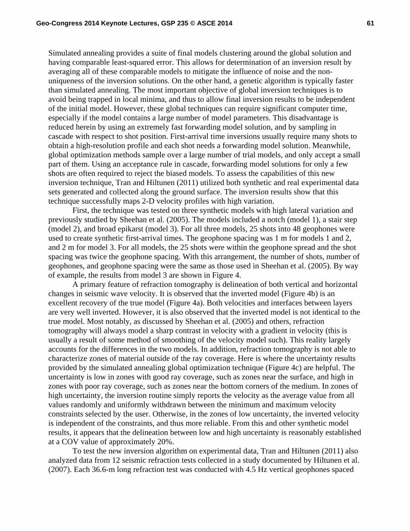
At station 19.8 m, the CPT tip resistance approached a large value of 30 MPa, and the test was terminated at a depth of about 9.2 m. Station 19.8 m is near the middle of a valley feature on the tomograms (Figure 5a), and the CPT tip terminates at a P-wave velocity of ±2000 m/s.

The sounding at 39.6 m was terminated before the tip resistance approached a large value because the CPT rod system was bending seriously to the south as penetration was attempted. It is interesting to note on the tomograms (Figure 6a) that station 39.6 m is slightly to the left of a block/pinnacle feature, and bending of the CPT rod to the south at the site (to the left or lower station number on tomogram) is consistent with this block feature.

At stations 44.2 and 65.5 m the tests were terminated at shallow depths less than 0.5 m because the CPT tip resistance approached a large value of 30 MPa. Stations 44.2 and 65.5 m are both located near the top of block/pinnacle features on the tomograms (Figure 6a). However, in contrast to station 19.8 m, the CPT tips terminated at P-wave velocities less than 1000 m/s at stations 44.2 and 65.5 m.

It is reported that small, rock outcrops were visible near stations 62.5-64 m and 66.1-67.1 m, which are on both sides of the CPT sounding at 65.5 m. In summary, it would appear that the CPT site characterization results provide corroborating

evidence for the refraction tomograms presented herein, and suggest that the refraction tomograms provide valuable information regarding subsurface characteristics. In addition, it is noted that a global optimization scheme based on simulated annealing and using an extremely fast forwarding model solution is feasible for practical engineering inversion problems. The inversion technique does not depend on the initial model, and rather than just one final model, simulated annealing provides a suite of final models clustering around the global minimum. The technique also can determine the uncertainties associated with inverted results. Combined Surface/Borehole. Utilizing the new inversion algorithm developed by Tran and Hiltunen (2011), the coupling of so-called downhole and refraction tomography techniques was presented by Tran and Hiltunen (2012a) as a geophysical means of improving the characterization of the material surrounding a borehole. Here a string of sensors is placed both horizontally along the ground surface and down a single borehole. With the sensors so located, energy is created and propagated from the ground surface and then detected via the sensor strings. Then two-dimensional or three-dimensional velocity structure is obtained by inverting the measured data via the Monte Carlo-based simulated annealing inversion scheme that provides a suite of accepted models clustering around the global minimum and having similar least-squared errors. These models are used to derive the inverted model and the associated quantitative uncertainty. The inversion results allow both qualitatively and quantitatively appraising the capabilities of the surface data as well as the combined data.

The proposed testing configuration was applied at a site located near Ft. McCoy, Florida, where an existing cased borehole was made available by the St. Johns River Water Management District. The site was documented to consist of soil over rock, with the top of bedrock at 12-m depth. The test was conducted to measure both surface and borehole data. The surface data were measured with vertical geophones equally spaced at every 1 m from 0 m to 30 m, for a total of 31 measurements. The borehole data were measured in a borehole installed at station 15 m with borehole geophones equally placed at every 1 m from 4 m to 18 m depth, for a total of 15 measurements. Seismic energy was generated by vertically striking a metal ground plate with a


13

sledgehammer, thus producing compression wave (P-wave) first arrivals. Shot locations were placed from 1 m to 3 m spacing along 30 m on the surface and starting from 0 m, for a total of 20 shots. The shot spacing was 1 m for shots close to the borehole, 2 m for shots farther, and 3 m for shots at both ends.

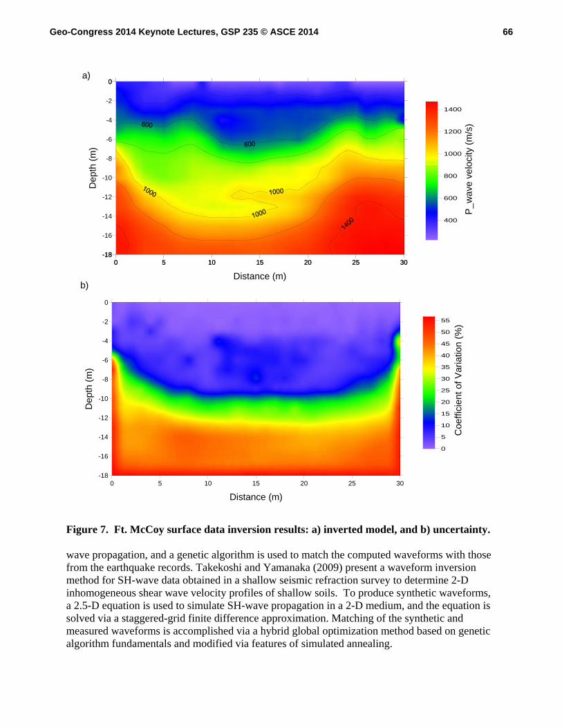
Figures 7a and 7b present the two-dimensional P-wave refraction tomogram determined from the travel-time data collected along the surface and the associated uncertainty. Because of noise, subjective judgments in manually picking first arrival times, and non-uniqueness of inverted solutions, the last 50,000 accepted models were used to derive the inverted profiles and the associated uncertainties. The tomogram (Figure 7a) indicates that the P-wave velocity generally increases with depth within the investigation area. The uncertainty (Figure 7b) is consistent with expectation, with low uncertainty in zones with good ray coverage and high uncertainty in zones with poor ray coverage. With the confidence gained from running synthetic models, the depth of investigation is about 10 m, where the COV from the surface to that depth is less than 20 percent. Thus, the surface data provide no information about the bedrock. Figures 8a and 8b show the P-wave tomogram and the associated uncertainty determined from combined test data collected along the surface and in the borehole. The inversion results indicate that the top of bedrock at 12-m depth is associated with a P-wave velocity contour of about 1200 m/s. This is consistent with the findings of Hiltunen and Cramer (2008), where pile tip elevations at driving refusal were typically at P-wave velocity contours of 1000 m/s to 1200 m/s.

Comparing the velocity profiles, Figure 7a against Figure 8a, the profiles are similar at shallow depth. This similarity is understandable because the shallow structure is mainly determined by the surface data, which is the same in both inversion runs. At deeper depth, the profiles are different because only the profile from the combined data is determined from the test measurement; the other is simply reported by inversion as an average of the minimum and maximum velocity constraints provided by the user. Similarly, a comparison of uncertainty results (Figure 7b against Figure 8b) indicates that the uncertainty is significantly reduced at depth for the case of using a borehole. Thus, the inversion results of the combined data can provide credible information well within the rock mass. Overall, the addition of a borehole significantly improves the resolution of the inverted profile, reduces the associated uncertainty, and increases the depth of investigation. Credible characterization of the bedrock is only obtained from the inversion of the combined data.

FULL WAVEFORM INVERSION

The surface wave and refraction tomography techniques presented above utilize only a

portion of the wavefield generated in a field test. Alternatively, the emerging technique of full waveform inversion (FWI) (Plessix 2008 and Vireux and Operto 2009) offers the potential to produce more detailed resolution of the subsurface by extracting information contained in the complete waveforms. As with refraction tomography, full waveform inversion has become possible due to advancements in wave propagation modeling, inversion algorithms, and modern computing.

While Vireux and Operto (2009) have indicated that linearized inversion algorithms are most commonly using in FWI for earth-scale models, two recent examples have utilized global optimization in matching full waveforms. Suzuki and Yamanaka (2008) present an inversion method for estimating 1-D shear wave velocity profiles using the shear wave arrivals extracted from earthquake records. The waveforms are calculated via the Haskell (1960) method for SH-


14

Figure 7. Ft. McCoy surface data inversion results: a) inverted model, and b) uncertainty. wave propagation, and a genetic algorithm is used to match the computed waveforms with those from the earthquake records. Takekoshi and Yamanaka (2009) present a waveform inversion method for SH-wave data obtained in a shallow seismic refraction survey to determine 2-D inhomogeneous shear wave velocity profiles of shallow soils. To produce synthetic waveforms, a 2.5-D equation is used to simulate SH-wave propagation in a 2-D medium, and the equation is solved via a staggered-grid finite difference approximation. Matching of the synthetic and measured waveforms is accomplished via a hybrid global optimization method based on genetic algorithm fundamentals and modified via features of simulated annealing.

0 5 10 15 20 25 30

Distance (m)

-18

-16

-14

-12

-10

-8

-6

-4

-2

0

Dep

th (

m)

0 5 10 15 20 25 30-18

0

P_w

ave

vel

ocity

(m

/s)

Coe

ffici

ent o

f Var

iatio

n (

%)

a)

b)

0 5 10 15 20 25 30

Distance (m)

-18

-16

-14

-12

-10

-8

-6

-4

-2

0

Dep

th (

m)

0

5

10

15

20

25

30

35

40

45

50

55

400

600

800

1000

1200

1400


15

Figure 8. Ft. McCoy combined data inversion results: a) inverted model, and b) uncertainty.

Tran and Hiltunen (2012b, 2012c) have investigated full waveform inversion (FWI) techniques that use the full information of elastic wavefields (body waves and surface waves) to potentially increase the resolution of inversion results. Like surface wave and seismic refraction tests, the wavefield is generated in the field by a vertical impact on the ground surface and recorded via receivers deployed along the surface in a linear array. The inversion scheme is based on a finite-difference solution of the 2-D elastic wave equation in the time-distance domain (Virieux 1986). Tran and Hiltunen (2012b, 2012c) have also utilized two global inversion techniques (genetic algorithm and simulated annealing) to invert the full wavefields for

0 5 10 15 20 25 30

Distance (m)

-18

-16

-14

-12

-10

-8

-6

-4

-2

0D

epth

(m

)

0 30

-16

0

P_w

ave

velo

city

(m

/s)

Coe

ffici

ent

of V

aria

tion

(%)

a)

b)

0 5 10 15 20 25 30

Distance (m)

-18

-16

-14

-12

-10

-8

-6

-4

-2

0

Dep

th (

m)

0

5

10

15

20

25

30

35

40

45

50

55

400

600

800

1000

1200

1400

1600

1800


16

near-surface velocity profiles by matching the observed and computed waveforms in the time domain. Typically, the inversion is specified to invert for both shear wave velocities and layer thicknesses, while the Poisson’s ratio and mass density of each layer remain constant. The goals of these initial studies were to assess whether full waveforms can provide sensitivity to both low- and high-velocity layers in laterally inhomogeneous materials, and whether full waveforms coupled with a global optimization technique is computationally practical, e.g., can a good model be found within a few hours of computing time.

The technique was tested on several synthetic data sets created from challenging models with both high-velocity and low-velocity layers at different depths, and two examples are shown below. Model 1 is a 1-D synthetic model that includes a low-velocity layer. The model is from Tokimatsu et al. (1992) and was previously used for studies of inversion using surface wave velocity dispersion by O’Neill, Dentith, and List (2003). Model 2 incorporates lateral variation and consists of multi-linear interfaces that require data from many receivers along the surface to accurately invert for the true profile. Finally, the technique is tested on an experimental data set and the inversion results are compared to other independent information. Synthetic Model 1. Model 1 consists of a buried low-velocity layer (second layer) between two high-velocity layers, followed by a half space (Figure 9). The observed waveforms were generated in Plaxis2D using 10 receivers at 4-m spacing on the surface, and a triangular impulsive load placed 4 m away from the first receiver. An analysis of the frequency-domain characteristics of the source and the resulting wavefield indicated that the source generates and the receiver signals contain energy up to frequencies of about 30 Hz, and the phase velocities of the wavefield vary from about 100 m/s to 500 m/s. Before inversion, the waveforms were low-pass filtered to remove signals larger than 30 Hz. In addition, in order to increase the contribution of the far-field signals, the receivers were treated equally by normalizing the maximum magnitude of the measured signals at each receiver to unity before being used for inversion, thus removing radiation damping in wave propagation.

Before running the genetic algorithm inversion, constraints, parameter coding, and model and grid sizes need to be specified. For velocity constraints, S-wave velocities were allowed to vary between 50 m/s and 300 m/s for the 3 layers, and between 50 m/s and 500 m/s for the half space. For thickness constraints, thicknesses were allowed to vary between 1 m and 5 m for layers 1 and 2, and between 5 m and 10 m for layer 3. With the selected constraints, all parameters are coded by 7 bits (0 or 1) that provide velocity resolution of less than 4 m/s, and thickness resolution of less than 0.04 m for all layers.

For the model and grid sizes, the model was selected as 20 m deep and 60 m wide. The width was extended 20 m horizontally from the last receiver to help limit the boundary affect during forward modeling. Based on the receiver spacing and the minimum true S-wave velocity, the grid size was specified as 0.5 m, which can accurately model the maximum frequency of about 30 Hz at which the criterion of 10 mesh points per wavelength is satisfied.

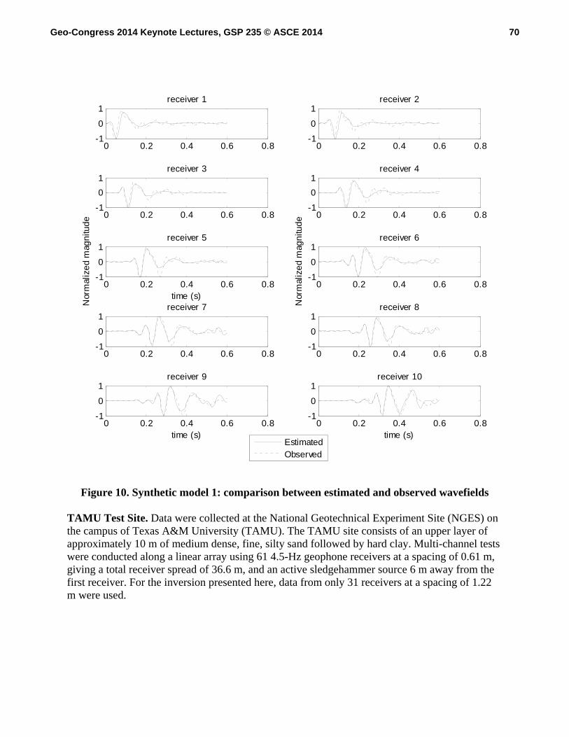
The inversion began with the first generation of 100 random models, and 100 generations were utilized to produce the inversion result. The run took about 2 hours on a laptop computer (2 GHz Pentium processor and 1 GB of memory). The inversion result was taken as the model of the final generation having the highest correlation. Figure 10 indicates that a good match between the observed data and estimated data is achieved with the inverted model, and a comparison of the inverted model against the true model presented in Figure 9 demonstrates that a good match is found.


17

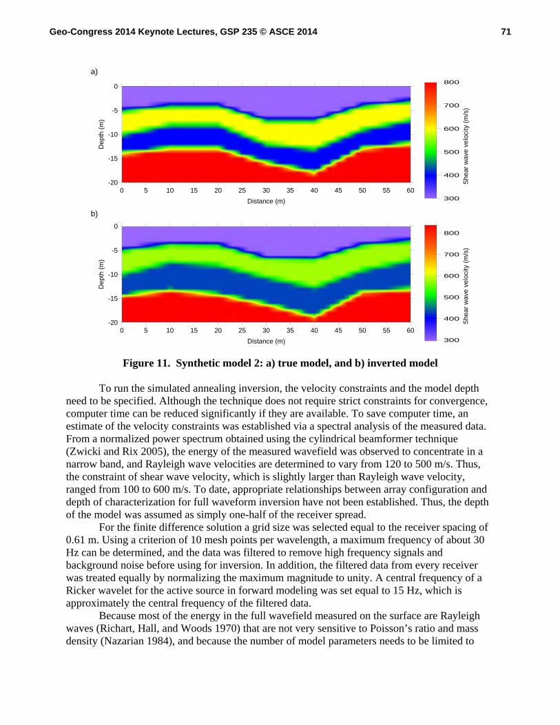
Figure 9. Synthetic model 1: comparison of the true and inverted models Synthetic Model 2. Model 2 consists of three low- and high-velocity layers followed by a half space, with six horizontal linear segments in each interface (Figure 11a). The observed waveforms were generated by the finite-difference forward model using 51 receivers at 1-m spacing on the surface, and an active source placed 10 m away from the first receiver. The active source was modeled as a Ricker wavelet having a central frequency of 15 Hz.

To run the simulated annealing inversion, the source, Poisson’s ratio, mass density, and the number of linear segments in each interface were kept the same as values used to generate the observed waveforms, thus the number of model parameters was 25 (7 thicknesses in each layer of the 3 layers, and 4 velocities). The velocity was allowed to vary between 200 m/s and 900 m/s, and the thickness was allowed to vary between 2 m and 10 m. The inversion began with the initial model of a constant velocity of 400 m/s, parameters were perturbed, and the temperature was reduced after 5000 accepted models until convergence. The run tested more than 150,000 trial models in about half a day on a standard laptop computer.

Figure 11b represents the inverted model, which was determined as the arithmetic average of the last 5000 accepted models at the final temperature. Good recovery of the true model is found: both layer velocities and interfaces are inverted with differences of less than 10% compared to those of the true model. A comparison of the observed and estimated waveforms indicated that the data has been well fit across the whole range of spatial offsets and the two wavefields are almost identical. Also, the accepted models in the simulated annealing were observed to cluster near to those of the true model.

Of course, this good recovery of the true model is aided by several assumptions: the finite difference solution was used to generate the observed wavefield and as the forward model during inversion, and the model for both the generation of observations and for inversion used the same Poisson’s ratio, mass density, and horizontal interface segments. However, the inversion result does demonstrate that it is possible using full waveforms from only one shot to characterize 2-D profiles with interfaces of linear segments of a few meters. .

-20.0

-18.0

-16.0

-14.0

-12.0

-10.0

-8.0

-6.0

-4.0

-2.0

0.0

0 100 200 300 400

Shear wave velocity (m/s)

Dep

th (

m)

True model

Inverted model


18

Figure 10. Synthetic model 1: comparison between estimated and observed wavefields

TAMU Test Site. Data were collected at the National Geotechnical Experiment Site (NGES) on the campus of Texas A&M University (TAMU). The TAMU site consists of an upper layer of approximately 10 m of medium dense, fine, silty sand followed by hard clay. Multi-channel tests were conducted along a linear array using 61 4.5-Hz geophone receivers at a spacing of 0.61 m, giving a total receiver spread of 36.6 m, and an active sledgehammer source 6 m away from the first receiver. For the inversion presented here, data from only 31 receivers at a spacing of 1.22 m were used.

0 0.2 0.4 0.6 0.8-1

0

1receiver 1

0 0.2 0.4 0.6 0.8-1

0

1receiver 2

0 0.2 0.4 0.6 0.8-1

0

1receiver 3

0 0.2 0.4 0.6 0.8-1

0

1receiver 4

0 0.2 0.4 0.6 0.8-1

0

1receiver 5

time (s)

Nor

mal

ize

d m

agnitu

de

0 0.2 0.4 0.6 0.8-1

0

1receiver 6

Nor

mal

ize

d m

agnitu

de

0 0.2 0.4 0.6 0.8-1

0

1receiver 7

0 0.2 0.4 0.6 0.8-1

0

1receiver 8

0 0.2 0.4 0.6 0.8-1

0

1receiver 9

time (s)0 0.2 0.4 0.6 0.8

-1

0

1receiver 10

time (s)

EstimatedObserved


19

Figure 11. Synthetic model 2: a) true model, and b) inverted model

To run the simulated annealing inversion, the velocity constraints and the model depth need to be specified. Although the technique does not require strict constraints for convergence, computer time can be reduced significantly if they are available. To save computer time, an estimate of the velocity constraints was established via a spectral analysis of the measured data. From a normalized power spectrum obtained using the cylindrical beamformer technique (Zwicki and Rix 2005), the energy of the measured wavefield was observed to concentrate in a narrow band, and Rayleigh wave velocities are determined to vary from 120 to 500 m/s. Thus, the constraint of shear wave velocity, which is slightly larger than Rayleigh wave velocity, ranged from 100 to 600 m/s. To date, appropriate relationships between array configuration and depth of characterization for full waveform inversion have not been established. Thus, the depth of the model was assumed as simply one-half of the receiver spread.

For the finite difference solution a grid size was selected equal to the receiver spacing of 0.61 m. Using a criterion of 10 mesh points per wavelength, a maximum frequency of about 30 Hz can be determined, and the data was filtered to remove high frequency signals and background noise before using for inversion. In addition, the filtered data from every receiver was treated equally by normalizing the maximum magnitude to unity. A central frequency of a Ricker wavelet for the active source in forward modeling was set equal to 15 Hz, which is approximately the central frequency of the filtered data.

Because most of the energy in the full wavefield measured on the surface are Rayleigh waves (Richart, Hall, and Woods 1970) that are not very sensitive to Poisson’s ratio and mass density (Nazarian 1984), and because the number of model parameters needs to be limited to

0 5 10 15 20 25 30 35 40 45 50 55 60

Distance (m)

-20

-15

-10

-5

0

De

pth

(m

)

300

400

500

600

700

800

She

ar w

ave

velo

city

(m

/s)

0 5 10 15 20 25 30 35 40 45 50 55 60

Distance (m)

-20

-15

-10

-5

0

Dep

th (

m)

300

400

500

600

700

800

She

ar

wa

ve v

elo

city

(m

/s)

a)

b)


20

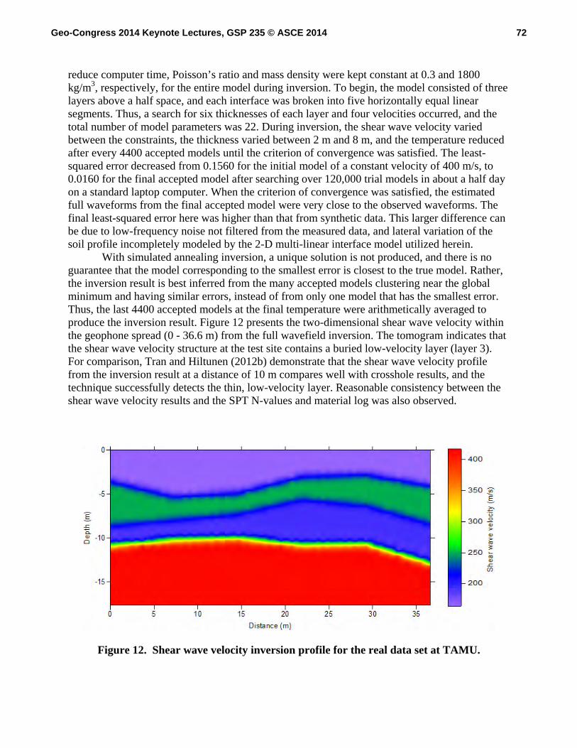
reduce computer time, Poisson’s ratio and mass density were kept constant at 0.3 and 1800 kg/m3, respectively, for the entire model during inversion. To begin, the model consisted of three layers above a half space, and each interface was broken into five horizontally equal linear segments. Thus, a search for six thicknesses of each layer and four velocities occurred, and the total number of model parameters was 22. During inversion, the shear wave velocity varied between the constraints, the thickness varied between 2 m and 8 m, and the temperature reduced after every 4400 accepted models until the criterion of convergence was satisfied. The least-squared error decreased from 0.1560 for the initial model of a constant velocity of 400 m/s, to 0.0160 for the final accepted model after searching over 120,000 trial models in about a half day on a standard laptop computer. When the criterion of convergence was satisfied, the estimated full waveforms from the final accepted model were very close to the observed waveforms. The final least-squared error here was higher than that from synthetic data. This larger difference can be due to low-frequency noise not filtered from the measured data, and lateral variation of the soil profile incompletely modeled by the 2-D multi-linear interface model utilized herein.

With simulated annealing inversion, a unique solution is not produced, and there is no guarantee that the model corresponding to the smallest error is closest to the true model. Rather, the inversion result is best inferred from the many accepted models clustering near the global minimum and having similar errors, instead of from only one model that has the smallest error. Thus, the last 4400 accepted models at the final temperature were arithmetically averaged to produce the inversion result. Figure 12 presents the two-dimensional shear wave velocity within the geophone spread (0 - 36.6 m) from the full wavefield inversion. The tomogram indicates that the shear wave velocity structure at the test site contains a buried low-velocity layer (layer 3). For comparison, Tran and Hiltunen (2012b) demonstrate that the shear wave velocity profile from the inversion result at a distance of 10 m compares well with crosshole results, and the technique successfully detects the thin, low-velocity layer. Reasonable consistency between the shear wave velocity results and the SPT N-values and material log was also observed.

Figure 12. Shear wave velocity inversion profile for the real data set at TAMU.


21

CONCLUSIONS

New developments in surface-based seismic wave methods are described around three significant themes: 1) array signal processing, 2) numerical methods for solving the equations of wave propagation, and 3) global optimization methods for solving the inverse problem. These themes are illustrated via examples from surface wave, refraction-based travel time, and full waveform inversion techniques.

A new generation of surface wave techniques based upon advancements in array signal processing are compared against more traditional methodologies at a test site in Florida. In particular, data from conventional active-source MASW, a new non-uniform active-source array, ReMi, and two dimensional (2D) passive-source arrays are compared. A non-uniform linear array of receivers together with a small vibration shaker significantly improves the resolution of dispersion curves as compared to conventional multi-channel sledgehammer source arrays, particularly at low frequencies. Inversion of the combined dispersion curve from a non-uniform active-source array and a 2D passive-source array yielded a significantly deeper shear wave velocity profile for the site than produced in a previous study using dispersion data from a sledgehammer source uniform array and ReMi.

Seismic refraction tomography techniques have provided a significant new geophysical tool that have been made possible by: 1) the coupling of efficient numerical methodologies to solve the relevant equations of wave propagation with modern computers, and 2) the utilization of optimization techniques to efficiently search the parameter space for plausible models to describe the subsurface. A global optimization scheme based on simulated annealing is presented to obtain near-surface velocity profiles from travel times. By using a fast forwarding model solution, the technique is feasible for practical engineering inversion problems. Simulated annealing provides a suite of final models clustering around the global solution and having comparable least-squared error. This provides an inversion result by averaging all of these accepted models to mitigate the influence of noise and the non-uniqueness of the inversion solutions. The technique also can determine the uncertainties associated with inverted results. A comparison of inversion results utilizing combined borehole and surface data against inversion results developed using just the surface data suggests that significant additional resolution of inverted profiles at depth are obtained, and uncertainties are significantly reduced with the addition of a borehole. This is particularly attractive for characterizing a rock mass underlying a surface soil layer. The surface wave and refraction tomography techniques utilize only a portion of the wavefield generated in a field test. Alternatively, the emerging technique of full waveform inversion (FWI) offers the potential to produce more detailed resolution of the subsurface by extracting information contained in the complete waveforms. As with refraction tomography, full waveform inversion has become possible due to advancements in wave propagation modeling, inversion algorithms, and modern computing. Techniques are presented to invert full waveforms using two global optimization methods, a genetic algorithm and simulated annealing. The inversion scheme is based on a finite-difference solution of the 2D elastic wave equation in the time-distance domain. The strength of this approach is the ability to generate all possible wave types and thus to simulate complex seismic wavefields that are then compared with observed data to infer subsurface properties. The capability of this inversion technique is tested with both synthetic and real experimental data sets. The inversion results from synthetic data show the ability of characterizing both low- and high-velocity layers, and the inversion results from real


22

data are generally consistent with crosshole, SPT N-value, and material log results, including the identification of a buried low-velocity layer. Based upon the cases presented, coupling of global optimization with full waveforms is computationally practical, as the results presented herein were all achieved on a standard laptop computer. ACKNOWLEDGEMENTS

Much of the work described herein was supported by the Florida Department of Transportation, and the authors thank David Horhota, Peter Lai, Larry Jones, Brian Bixler, and Rodrigo Herrera for their technical support and encouragement. REFERENCES Carpenter, P. J., Higuera-Diaz, I. C., Thompson, M. D., Atre, S., and Mandell, W. (2003),

“Accuracy of Seismic Refraction Tomography Codes at Karst Sites,” Geophysical Site Characterization: Seeing Beneath the Surface, Proceedings of a Symposium on the Application of Geophysics to Engineering and Environmental Problems, San Antonio, Texas, April 6-10, pp. 832-840.

Chopp, D.L., 2001, Some improvements on Fast Marching Method: SIAM Journal on Scientific Computing, 23(1), 230-244.

Dijkstra, E.W., 1959, A note on two problems in connection with graphs: Journal of Numerical Mathematics, 1, 269-271.

Haskell, N. A., 1960, Crustal reflection of plane SH waves: Journal of Geophysical Research, 65, 4147-4150

Hassouna, M.S., and Farag, A.A., 2007, Multistencils Fast Marching Methods: A Highly Accurate Solution to the Eikonal Equation on Cartesian Domains: IEEE Transactions on Pattern Analysis and Machine Intelligence, 29(9), 1-12.

Hebeler, G. L. (2001), “Site Characterization in Shelby County, Tennessee Using Advanced Surface Wave Methods,” M.S. Thesis, Georgia Institute of Technology.

Hiltunen, D. R. and Cramer, B. J. (2008). “Application of seismic refraction tomography in karst terrane.” Journal of Geotechnical and Geoenvironmental Engineering, 134(7), 938-948.

Hiltunen, D. R., Hudyma, N., Quigley, T. P., and Samakur, C. (2007), “Ground Proving Three Seismic Refraction Tomography Programs,” Transportation Research Record: Journal of the Transportation Research Board, No. 2016, Washington, D.C., pp. 110-120.

Kim, S., 1999, ENO-DNO-PS: A stable, Second-Order Accuracy Eikonal Solver: The Society of Exploration Geophysicists, 1747-1750.

Li, J. (2008), “Study of Surface Wave Methods for Deep Shear Wave Velocity Profiling Applied to the Deep Sediments of the Mississippi Embayment,” Ph.D. Dissertation, University of Missouri.

Louie, J. N., 2001, Faster, better, shear-wave velocity to 100 meters depth from refraction microtremor arrays: Bulletin of Seismological Society of America, 91(2), 347-364.

Moser, T.J., 1991, Shortest path calculation of seismic rays: Geophysics, 56, 59-67. Nakanishi, J., and Yamaguchi, K., 1986, A numerical experiment on non-linear image

reconstruction from first arrival times for two-dimensional island structure: Journal of Physics of the Earth, 34, 195-201.


23

Nazarian, S., 1984, In situ determination of elastic moduli of soil deposits and pavement systems by spectral-analysis-of-surface-waves method: Ph.D. Dissertation, The University of Texas at Austin.

Nichols, D.E., 1996, Maximum energy travel times calculated in seismic frequency band: Geophysics, 61, 253-263.

O’Neill, A., Dentith, M., and List, R. (2003), Full-waveform P-SV reflectivity inversion of surface waves for shallow engineering applications: Exploration Geophysics, 34(3), 158-173.

Park, C. B., Miller, R. D., and Xia, J., 1999, Multi-channel analysis of surface wave (MASW): Geophysics, 64(3), 800-808.

Plessix, R. E., 2008, Introduction: Towards a full waveform inversion: Geophysical Prospecting, 56, 761-763.

Powell, G.E. and Whiteley, R.J. (2008) “Prediction of Piling Conditions in Genting Highlands Granites, Malaysia with borehole seismic imaging,” Geotechnical and Geophysical Site Characterization, Proceedings of the 3rd International Conference on Site Characterization, Taipei, Taiwan, April 1-4, pp. 925-928.

Pullammanappallil, S.K., and Louie, J.N., 1994, A generalized simulated annealing optimization for inversion of first arrival time: Bulletin of the Seismological Society of America, 84(5), 1397-1409.

Richart, F. E., Jr., Hall, J. R., Jr., and Woods, R. D., 1970, Vibrations of Soils and Foundations, Prentice-Hall, Inc., Englewood Cliffs, New Jersey, 414 pp.

Rosenblad, B. L., and Li, J. (2009), “Performance of Active and Passive Methods for Measuring Low-Frequency Surface Wave Dispersion Curves, Journal of Geotechnical and Geoenvironmental Engineering, American Society of Civil Engineers, Vol. 135, No. 10, October, pp. 1419-1428.

Sambridge, M. and Mosegaard, K. (2002), Monte Carlo methods in geophysical inverse problems: Reviews of Geophysics, 40(3).

Sen, M.K. and Stoffa, P.L. (1991), Nonlinear multiparameter optimization using genetic algorithms: Inversion of plane-wave seismograms: Geophysics, 56 (11), 1794-1810.

Sen, M.K. and Stoffa, P.L. (1995), Global optimization methods in geophysical inversion: Adv. Explor. Geophysics, Vol. 4, Elsevier Sci., New York.

Sethian, J.A., 1996, Fast Marching Set Level Method for Monotonically Advancing Fronts: Proceedings of the National Academy of Sciences, Vol. 93.

Sethian, J.A., 1999, Level Set Methods and Fast Marching Methods: 2nd ed. Campridge University Press.

Sharma, S.P. and Kaikkonen, P. (1998), Two-dimensional non-linear inversion of VLF-R data using simulated annealing: Geophysics J, Int. 133, 649-668.

Sheehan, J.R., Doll, W.E., and Mandell, W.A., 2005, An Evaluation of Methods and Available Software for Seismic Refraction Tomography Analysis: Journal of Environmental and Engineering Geophysics, 10, 21-34.

Suzuki, H. and Yamanaka, H., 2008, Estimation of S-wave velocity structure of deep soils using waveform inversion for S-wave part of earthquake ground motion from small event: The 14th World Conference on Earthquake Engineering, Beijing, China, October 12-17.

Takekoshi, M. and Yamanaka, H., 2009, Waveform inversion of shallow seismic refraction data using hybrid heuristic search method: Exploration Geophysics, 40, 99-104.


24

Tokimatsu, K., Tamura, S., and Kojima, H. (1992), Effects of multiple modes on Rayleigh wave dispersion characteristics: Journal of Geotechnical and Geoenvironmental Engineering, 118 (2), 1529–1543.

Tran, K. T. and Hiltunen, D. R., 2008, A comparison of shear wave velocity profiles from SASW, MASW, and ReMi techniques: Geotechnical Earthquake Engineering and Soil Dynamics IV, Geotechnical Special Publication No. 181, D. Zeng, M. T. Manzari, and D. R. Hiltunen, Eds., American Society of Civil Engineers.

Tran, K. T. and Hiltunen, D. R. (2011), “Inversion of First-Arrival Time Using Simulated Annealing,” Journal of Environmental and Engineering Geophysics, Environmental and Engineering Geophysical Society, Vol. 16, No. 1, March, pp. 25-35.

Tran, K. T. and Hiltunen, D. R. (2012a), “Inversion of Combined Surface and Borehole First-Arrival Time,” Journal of Geotechnical and Geoenvironmental Engineering, American Society of Civil Engineers, Vol. 138, No. 3, March, pp. 272-280.

Tran, K. T. and Hiltunen, D. R. (2012b), “Two-Dimensional Inversion of Full Waveforms Using Simulated Annealing,” Journal of Geotechnical and Geoenvironmental Engineering, American Society of Civil Engineers, Vol. 138, No. 9, September, pp. 1075-1090.

Tran, K. T. and Hiltunen, D. R. (2012c), “One-Dimensional Inversion of Full Waveforms Using a Genetic Algorithm,” Journal of Environmental and Engineering Geophysics, Environmental and Engineering Geophysical Society, Vol. 17, No. 4, December, pp.197-213.

Van Trier, J., and Symes, W., 1991, Upwind finite-difference calculation of travel times: Geophysics, 56, 812-821.

Vidale, J.E., 1988, Finite-difference travel time calculation: Bulletin of the Seismological Society of America, 78, 2062-2076.

Virieux, J. (1986), P-SV wave propagation in heterogeneous media: Velocity-stress finite-difference method: Geophysics, 51(4), 889-901.

Vireux, J. and Operto, S., 2009, An overview of full-waveform inversion in exploration geophysics: Geophysics, 74(6), WCC1-WCC26.

Whiteley, R.J. (2012), “Surface and borehole seismic imaging of soft-rock, karst eolianites at coastal engineering construction sites: case studies from Australia,” The Leading Edge, January, pp. 936-941.

Yoon, S. (2005). “Array-based measurements of surface wave dispersion and attenuation using frequency-wavenumber analysis.” Ph.D. dissertation, the Georgia Institute of Technology.

Zelt, C.A., Haines, S., Powers, M.H., Sheehan, J., Rohdewald, S., Link, C., Hayashi, K., Zhao, D., Zhou, H.W., Burton, B., Petersen, U.K., Bonal, N.D., and Doll, W.E. (2013), “Blind Tests of Methods for Obtaining 2-D Near-Surface Seismic Velocity Models from First-Arrival Traveltimes,” Journal of Environmental and Engineering Geophysics, Environmental and Engineering Geophysical Society, Vol. 18, No. 3, September, pp.183-194.

Zywicki, D. J. (1999), “Advanced Signal Processing Methods Applied to Engineering Analysis of Seismic Surface Waves,” Ph.D. Thesis, Georgia Institute of Technology, 357 pp.

Zywicki, D. J. and Rix, G. J. (2005). “Mitigation of Near-Field Effects for Seismic Surface WaveVelocity Estimation with Cylindrical Beamformers.” Journal of Geotechnical and Geoenvironmental Engineering, 131(8), 970-977.


978-0-7844-1329-6.003

Documents

surfacebased techniques

seismic wave methods

surface data

wave evaluation techniques

waveform inversion techniques

ground surface

global optimization

inversion scheme