6. non-linear pseudo-static analysis of...
TRANSCRIPT
6. NON-LINEAR PSEUDO-STATIC ANALYSIS OF ADOBE WALLS
Blondet et al. [2005] carried out a cyclic test on an adobe wall to reproduce its seismic response and damage pattern under in-plane loads. The displacement was applied at the wall top and at low increments to simulate a static analysis. In this work, the force-displacement curve obtained from the experimental test (see section 3.5) is used for calibrating preliminary numerical models of adobe walls.
In the previous chapter different modelling approaches were described for representing the cracking and damage on concrete panels, which are also applied to masonry panels, including adobe walls. These numerical approaches are divided into discrete and continuum models.
The numerical modelling of adobe structures is not simple since there is scarce material information, especially the fracture energy in tension and compression for modelling the inelastic behaviour of the adobe material. In this chapter three finite element models of adobe walls are built and, taking advantage of the experimental results shown in 3.5.3, the adobe material properties are calibrated within a discrete and continuum approach. For this, two finite element programmes are used: Midas FEA and Abaqus/Standard. In Midas FEA two finite element models are built, one following the simplified micro-modelling (discrete model) and the second one following a smeared crack model (continuum model). The adobe wall built in Abaqus/Standard is modelled following a damaged plasticity model (continuum model). The finite element models are solved following an implicit solution, and are described as follows.
6.1 IMPLICIT SOLUTION METHOD FOR SOLVING QUASI-STATIC PROBLEMS
In this analysis the load/displacement is applied slowly to the body so that the inertial forces can be neglected (acceleration and velocities are zero). It follows that the internal forces I (for a given displacement u ) must be equal to the external forces P at each time step t , or the residual force R u must be:
R u = P I u 0 (6.1)

Sabino Nicola Tarque Ruíz
114
Amongst the different solution procedures used in the implicit finite element solvers, the Newton-Raphson solution procedure is the faster for solving non-linear problems under force control, though no convergence procedure is full proof. When solving quasi static problems, a set of non-linear equations are generally expressed as:
T TV S
dV dS 0G u B u N t (6.2)
where G is a set of non-linear equations in u which are updated at each iteration and are function of the nodal displacements vector u , is the stresses vector, B is the matrix that relates the strain vector to the displacements, N is the matrix of element shape functions and t is the surface traction vector. V and S represent the volume and surface of the body, respectively. The right-hand side of Equation (6.2) represents the difference between the internal and the external forces.
Equation (6.2) is solved for a displacement vector that equilibrates the internal and external forces, as explained in Harewood and McHugh [2007]. Besides, Equation (6.2) is solved by incremental methods where load/displacements are applied in time steps t ,
t tu is solved from a known state tu . In the following equations the subscript denotes iteration number and the superscript denotes an increment step.
At the beginning, Equation (6.2) is solved to obtain the displacement correction t ti 1u
based on information of t tiu as:
t tit t t t
i i
1
1
G uu G u
u (6.3)
The partial derivative on the right side is the so called Jacobian matrix expressed as the global stiffness matrix tanK :
t tit t
itan
G uK u =
u (6.4)
Thus:
t t t t t ti i i
1
1 tanu K u G u (6.5)
The previous equation involves the inversion of the global stiffness matrix (no singular matrix), which ends in a computationally expensive operation, but it ensures that a
Numerical modelling of the seismic behaviour of adobe buildings
115
relatively large time increment can be used while maintaining the accuracy of the solution [Harewood and McHugh 2007].
The displacement correction t ti 1u is added to the previous state, thus the improved
displacement solution is given with Equation (6.6) and t ti 1u is used as the current
approximation to the solution for the subsequent iteration i 1 in Equation (6.2) until the equilibrium is reached.
t t t t t ti i i1 1u u u (6.6)
Convergence is measured by ensuring that the difference between external and internal forces G u , displacement increment t t
iu and displacement correction t ti 1u are
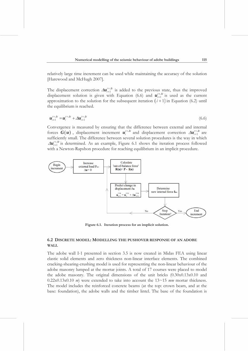
sufficiently small. The difference between several solution procedures is the way in which t ti 1u is determined. As an example, Figure 6.1 shows the iteration process followed
with a Newton-Rapshon procedure for reaching equilibrium in an implicit procedure.
Figure 6.1. Iteration process for an implicit solution.
6.2 DISCRETE MODEL: MODELLING THE PUSHOVER RESPONSE OF AN ADOBE
WALL
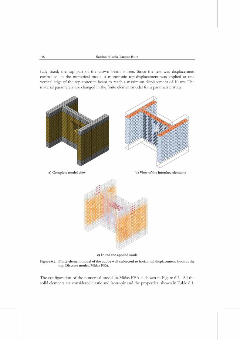
The adobe wall I-1 presented in section 3.5 is now created in Midas FEA using linear elastic solid elements and zero thickness non-linear interface elements. The combined cracking-shearing-crushing model is used for representing the non-linear behaviour of the adobe masonry lumped at the mortar joints. A total of 17 courses were placed to model the adobe masonry. The original dimensions of the unit bricks (0.30x0.13x0.10 and 0.22x0.13x0.10 m) were extended to take into account the 13~15 mm mortar thickness. The model includes the reinforced concrete beams (at the top: crown beam, and at the base: foundation), the adobe walls and the timber lintel. The base of the foundation is
Sabino Nicola Tarque Ruíz
116
fully fixed; the top part of the crown beam is free. Since the test was displacement controlled, in the numerical model a monotonic top-displacement was applied at one vertical edge of the top concrete beam to reach a maximum displacement of 10 mm. The material parameters are changed in the finite element model for a parametric study.
a) Complete model view b) View of the interface elements
c) In red the applied loads
Figure 6.2. Finite element model of the adobe wall subjected to horizontal displacement loads at the top. Discrete model, Midas FEA.
The configuration of the numerical model in Midas FEA is shown in Figure 6.2.. All the solid elements are considered elastic and isotropic and the properties, shown in Table 6.1,
Numerical modelling of the seismic behaviour of adobe buildings
117
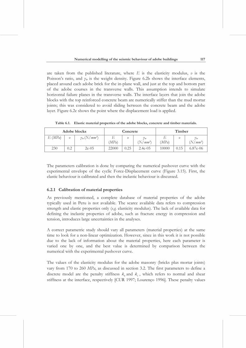
are taken from the published literature, where E is the elasticity modulus, is the Poisson’s ratio, and m is the weight density. Figure 6.2b shows the interface elements, placed around each adobe brick for the in-plane wall, and just at the top and bottom part of the adobe courses in the transverse walls. This assumption intends to simulate horizontal failure planes in the transverse walls. The interface layers that join the adobe blocks with the top reinforced concrete beam are numerically stiffer than the mud mortar joints; this was considered to avoid sliding between the concrete beam and the adobe layer. Figure 6.2c shows the point where the displacement load is applied.
Table 6.1. Elastic material properties of the adobe blocks, concrete and timber materials.
Adobe blocks Concrete Timber
E (MPa) m (N/mm3) E (MPa)
m (N/mm3)
E (MPa)
m (N/mm3)
230 0.2 2e-05 22000 0.25 2.4e-05 10000 0.15 6.87e-06
The parameters calibration is done by comparing the numerical pushover curve with the experimental envelope of the cyclic Force-Displacement curve (Figure 3.15). First, the elastic behaviour is calibrated and then the inelastic behaviour is discussed.
6.2.1 Calibration of material properties
As previously mentioned, a complete database of material properties of the adobe typically used in Peru is not available. The scarce available data refers to compression strength and elastic properties only (e.g. elasticity modulus). The lack of available data for defining the inelastic properties of adobe, such as fracture energy in compression and tension, introduces large uncertainties in the analyses.
A correct parametric study should vary all parameters (material properties) at the same time to look for a non-linear optimization. However, since in this work it is not possible due to the lack of information about the material properties, here each parameter is varied one by one, and the best value is determined by comparison between the numerical with the experimental pushover curve.
The values of the elasticity modulus for the adobe masonry (bricks plus mortar joints) vary from 170 to 260 MPa, as discussed in section 3.2. The first parameters to define a discrete model are the penalty stiffness nk and sk , which refers to normal and shear stiffness at the interface, respectively [CUR 1997; Lourenço 1996]. These penalty values
Sabino Nicola Tarque Ruíz
118
are related to the elasticity modulus of the adobe bricks and the mortar joints, as seen in Equation (5.12) and repeated here for convenience:
unit mortarn
mortar unit mortar
E Ekh E E
(6.7)
unit mortars
mortar unit mortar
G Gkh G G
(6.8)
The elasticity modulus for the adobe bricks is assumed as 230 MPa. The elasticity modulus for the mud mortar is assumed to be lower than that for bricks, so values of 79.25, 113.40, 156.50 and 216.85 MPa are considered. The mortar thickness, mortarh , is around 15 mm. The shear modulus is taken as 0.4E for the bricks and mortar. With the previous values, the normal and shear penalty stiffness are those reported in Table 6.2.
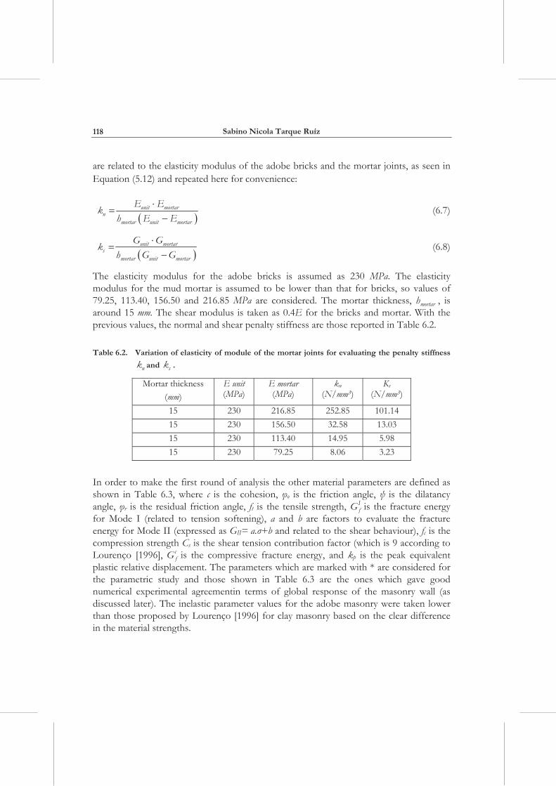
Table 6.2. Variation of elasticity of module of the mortar joints for evaluating the penalty stiffness
nk and sk .
Mortar thickness (mm)
E unit (MPa)
E mortar (MPa)
kn (N/mm3)
Ks (N/mm3)
15 230 216.85 252.85 101.14 15 230 156.50 32.58 13.03 15 230 113.40 14.95 5.98 15 230 79.25 8.06 3.23
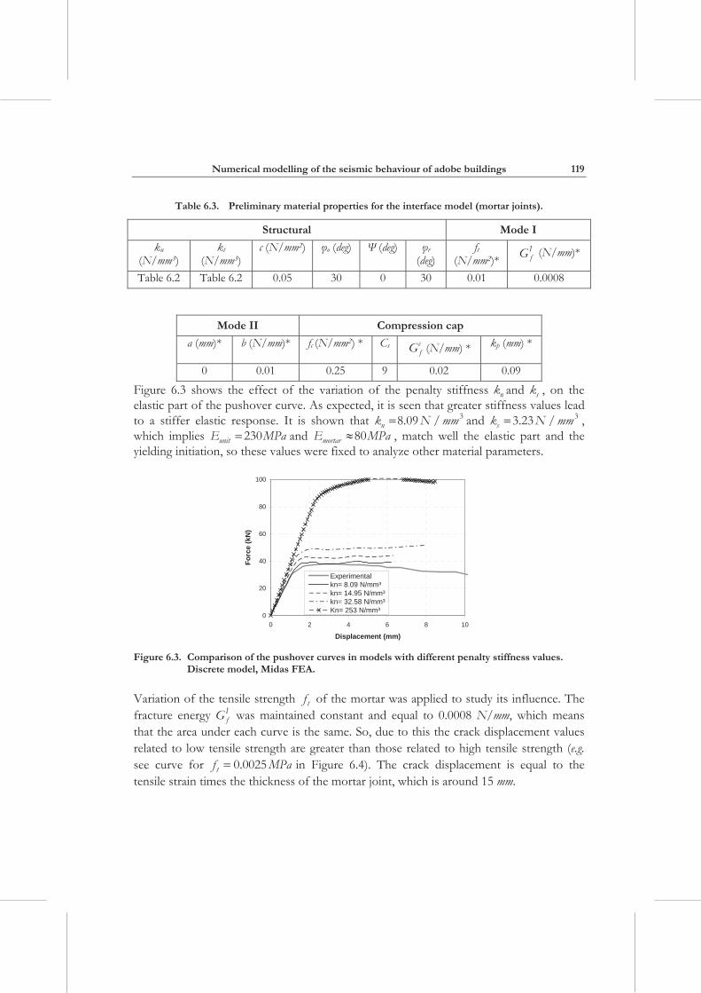
In order to make the first round of analysis the other material parameters are defined as shown in Table 6.3, where c is the cohesion, o is the friction angle, is the dilatancy angle, r is the residual friction angle, ft is the tensile strength, I
fG is the fracture energy for Mode I (related to tension softening), a and b are factors to evaluate the fracture energy for Mode II (expressed as GII= a. +b and related to the shear behaviour), fc is the compression strength Cs is the shear tension contribution factor (which is 9 according to Lourenço [1996], c
fG is the compressive fracture energy, and kp is the peak equivalent plastic relative displacement. The parameters which are marked with * are considered for the parametric study and those shown in Table 6.3 are the ones which gave good numerical experimental agreementin terms of global response of the masonry wall (as discussed later). The inelastic parameter values for the adobe masonry were taken lower than those proposed by Lourenço [1996] for clay masonry based on the clear difference in the material strengths.
Numerical modelling of the seismic behaviour of adobe buildings
119
Table 6.3. Preliminary material properties for the interface model (mortar joints).
Structural Mode I
kn (N/mm3)
kt (N/mm3)
c (N/mm2) o (deg) (deg) r (deg)
ft (N/mm2)*
IfG (N/mm)*
Table 6.2 Table 6.2 0.05 30 0 30 0.01 0.0008
Mode II Compression cap
a (mm)* b (N/mm)* fc (N/mm2) * Cs cfG (N/mm) * kp (mm) *
0 0.01 0.25 9 0.02 0.09
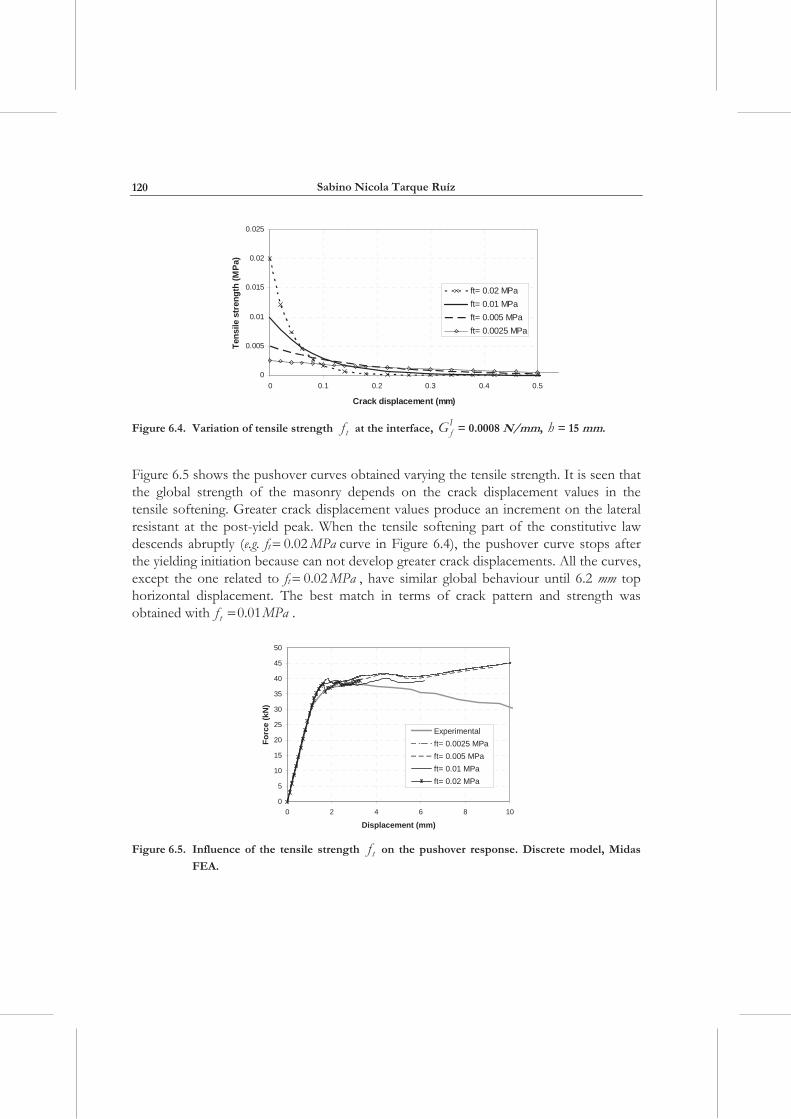
Figure 6.3 shows the effect of the variation of the penalty stiffness nk and sk , on the elastic part of the pushover curve. As expected, it is seen that greater stiffness values lead to a stiffer elastic response. It is shown that nk N mm38.09 / and sk N mm33.23 / , which implies unitE MPa230 and mortarE MPa80 , match well the elastic part and the yielding initiation, so these values were fixed to analyze other material parameters.
0
20
40
60
80
100
0 2 4 6 8 10
Displacement (mm)
Forc
e (k
N)
Experimentalkn= 8.09 N/mm³kn= 14.95 N/mm³kn= 32.58 N/mm³Kn= 253 N/mm³
Figure 6.3. Comparison of the pushover curves in models with different penalty stiffness values.
Discrete model, Midas FEA.
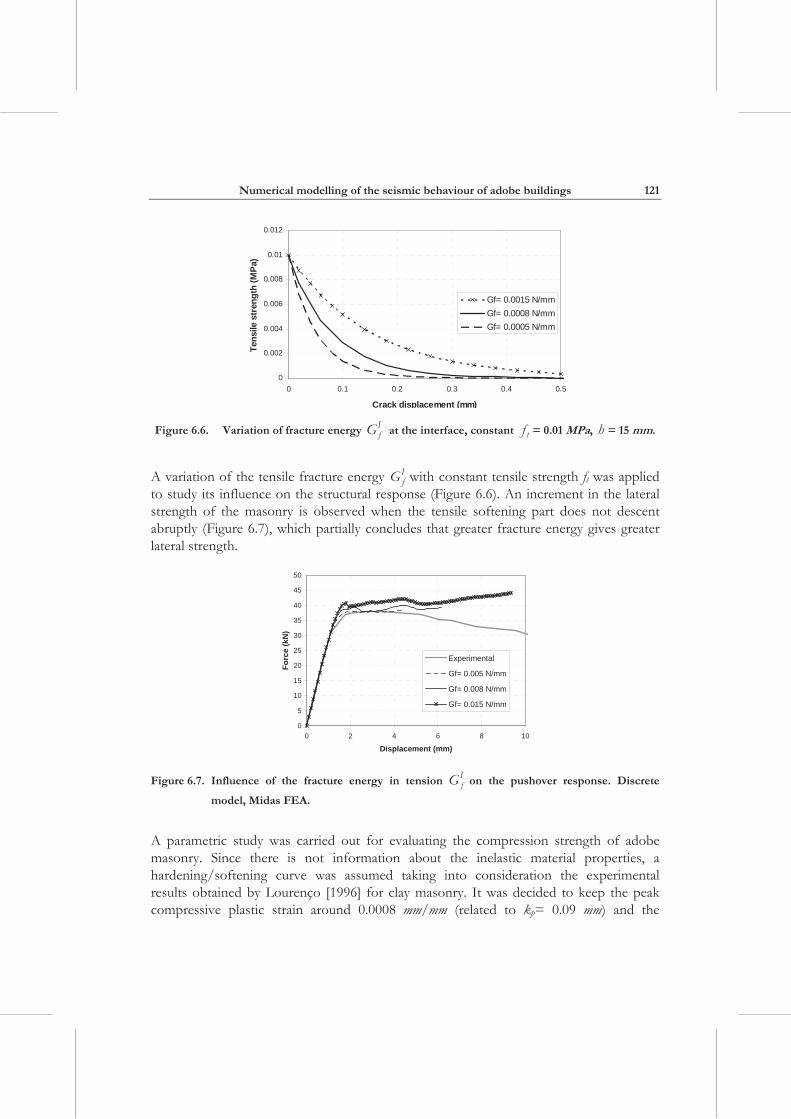
Variation of the tensile strength tf of the mortar was applied to study its influence. The fracture energy I
fG was maintained constant and equal to 0.0008 N/mm, which means that the area under each curve is the same. So, due to this the crack displacement values related to low tensile strength are greater than those related to high tensile strength (e.g. see curve for tf MPa0.0025 in Figure 6.4). The crack displacement is equal to the tensile strain times the thickness of the mortar joint, which is around 15 mm.
Sabino Nicola Tarque Ruíz
120
0
0.005
0.01
0.015
0.02
0.025
0 0.1 0.2 0.3 0.4 0.5
Crack displacement (mm)
Tens
ile s
tren
gth
(MPa
)
ft= 0.02 MPaft= 0.01 MPaft= 0.005 MPaft= 0.0025 MPa
Figure 6.4. Variation of tensile strength tf at the interface, IfG = 0.0008 N/mm, h = 15 mm.
Figure 6.5 shows the pushover curves obtained varying the tensile strength. It is seen that the global strength of the masonry depends on the crack displacement values in the tensile softening. Greater crack displacement values produce an increment on the lateral resistant at the post-yield peak. When the tensile softening part of the constitutive law descends abruptly (e.g. ft MPa0.02 curve in Figure 6.4), the pushover curve stops after the yielding initiation because can not develop greater crack displacements. All the curves, except the one related to ft MPa0.02 , have similar global behaviour until 6.2 mm top horizontal displacement. The best match in terms of crack pattern and strength was obtained with tf MPa0.01 .
0
5
10
15
20
25
30
35
40
45
50
0 2 4 6 8 10
Displacement (mm)
Forc
e (k
N)
Experimentalft= 0.0025 MPaft= 0.005 MPaft= 0.01 MPaft= 0.02 MPa
Figure 6.5. Influence of the tensile strength tf on the pushover response. Discrete model, Midas
FEA.
Numerical modelling of the seismic behaviour of adobe buildings
121
0
0.002
0.004
0.006
0.008
0.01
0.012
0 0.1 0.2 0.3 0.4 0.5
Crack displacement (mm)
Tens
ile s
tren
gth
(MPa
)
Gf= 0.0015 N/mmGf= 0.0008 N/mmGf= 0.0005 N/mm
Figure 6.6. Variation of fracture energy IfG at the interface, constant tf = 0.01 MPa, h = 15 mm.
A variation of the tensile fracture energy IfG with constant tensile strength ft was applied
to study its influence on the structural response (Figure 6.6). An increment in the lateral strength of the masonry is observed when the tensile softening part does not descent abruptly (Figure 6.7), which partially concludes that greater fracture energy gives greater lateral strength.
0
5
10
15
20
25
30
35
40
45
50
0 2 4 6 8 10
Displacement (mm)
Forc
e (k
N)
Experimental
Gf= 0.005 N/mm
Gf= 0.008 N/mm
Gf= 0.015 N/mm
Figure 6.7. Influence of the fracture energy in tension IfG on the pushover response. Discrete
model, Midas FEA.
A parametric study was carried out for evaluating the compression strength of adobe masonry. Since there is not information about the inelastic material properties, a hardening/softening curve was assumed taking into consideration the experimental results obtained by Lourenço [1996] for clay masonry. It was decided to keep the peak compressive plastic strain around 0.0008 mm/mm (related to kp= 0.09 mm) and the
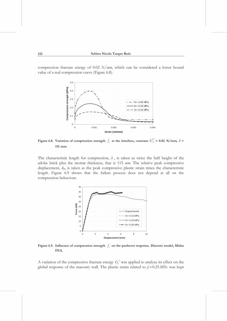
Sabino Nicola Tarque Ruíz
122
compression fracture energy of 0.02 N/mm, which can be considered a lower bound value of a real compression curve (Figure 6.8).
0
0.1
0.2
0.3
0.4
0.5
0 0.001 0.002 0.003 0.004
Strain (mm/mm)
Com
pres
sion
str
engt
h (M
Pa)
fc= 0.40 MPafc= 0.25 MPafc= 0.15 MPa
Figure 6.8. Variation of compression strength cf at the interface, constant CfG = 0.02 N/mm, h =
115 mm.
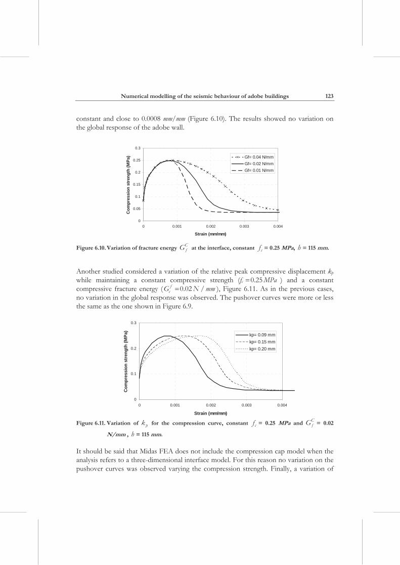
The characteristic length for compression, h , is taken as twice the half height of the adobe brick plus the mortar thickness, that is 115 mm. The relative peak compressive displacement, kp, is taken as the peak compressive plastic strain times the characteristic length. Figure 6.9 shows that the failure process does not depend at all on the compression behaviour.
0
5
10
15
20
25
30
35
40
45
0 2 4 6 8 10
Displacement (mm)
Forc
e (k
N)
Experimental
fc= 0.15 MPa
fc= 0.25 MPa
fc= 0.40 MPa
Figure 6.9. Influence of compression strength cf on the pushover response. Discrete model, Midas
FEA.
A variation of the compressive fracture energy fcG was applied to analyze its effect on the
global response of the masonry wall. The plastic strain related to fc MPa0.25 was kept
Numerical modelling of the seismic behaviour of adobe buildings
123
constant and close to 0.0008 mm/mm (Figure 6.10). The results showed no variation on the global response of the adobe wall.
0
0.05
0.1
0.15
0.2
0.25
0.3
0 0.001 0.002 0.003 0.004
Strain (mm/mm)
Com
pres
sion
str
engt
h (M
Pa) Gf= 0.04 N/mm
Gf= 0.02 N/mmGf= 0.01 N/mm
Figure 6.10. Variation of fracture energy CfG at the interface, constant cf = 0.25 MPa, h = 115 mm.
Another studied considered a variation of the relative peak compressive displacement kp
while maintaining a constant compressive strength (fc MPa0.25 ) and a constant compressive fracture energy ( f
cG N mm0.02 / ), Figure 6.11. As in the previous cases, no variation in the global response was observed. The pushover curves were more or less the same as the one shown in Figure 6.9.
0
0.1
0.2
0.3
0 0.001 0.002 0.003 0.004
Strain (mm/mm)
Com
pres
sion
str
engt
h (M
Pa)
kp= 0.09 mmkp= 0.15 mmkp= 0.20 mm
Figure 6.11. Variation of pk for the compression curve, constant cf = 0.25 MPa and C
fG = 0.02
N/mm , h = 115 mm.
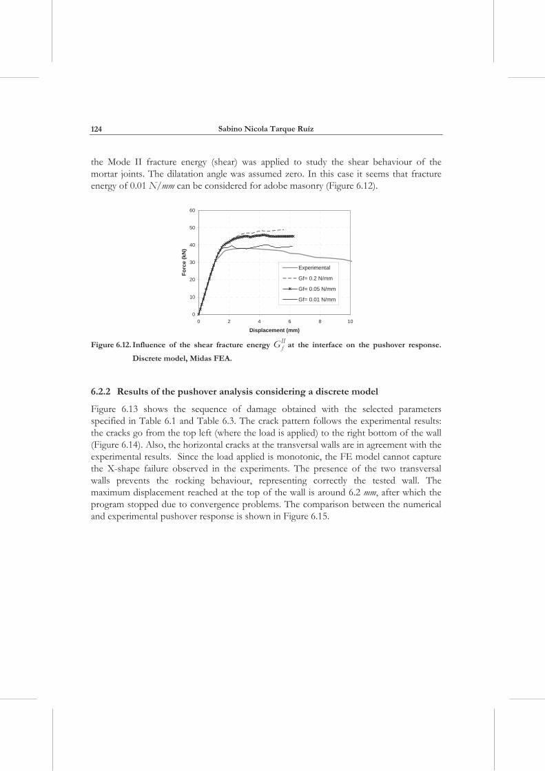
It should be said that Midas FEA does not include the compression cap model when the analysis refers to a three-dimensional interface model. For this reason no variation on the pushover curves was observed varying the compression strength. Finally, a variation of
Sabino Nicola Tarque Ruíz
124
the Mode II fracture energy (shear) was applied to study the shear behaviour of the mortar joints. The dilatation angle was assumed zero. In this case it seems that fracture energy of 0.01 N/mm can be considered for adobe masonry (Figure 6.12).
0
10
20
30
40
50
60
0 2 4 6 8 10
Displacement (mm)
Forc
e (k
N)
Experimental
Gf= 0.2 N/mm
Gf= 0.05 N/mm
Gf= 0.01 N/mm
Figure 6.12. Influence of the shear fracture energy II
fG at the interface on the pushover response.
Discrete model, Midas FEA.
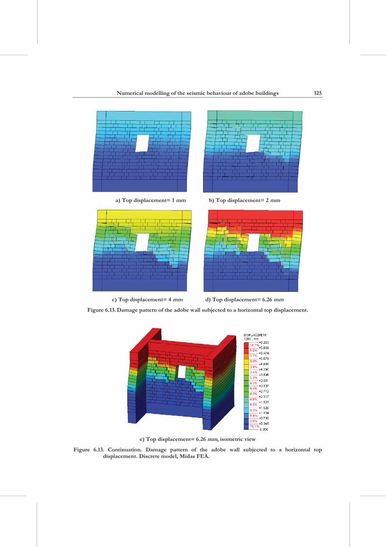
6.2.2 Results of the pushover analysis considering a discrete model
Figure 6.13 shows the sequence of damage obtained with the selected parameters specified in Table 6.1 and Table 6.3. The crack pattern follows the experimental results: the cracks go from the top left (where the load is applied) to the right bottom of the wall (Figure 6.14). Also, the horizontal cracks at the transversal walls are in agreement with the experimental results. Since the load applied is monotonic, the FE model cannot capture the X-shape failure observed in the experiments. The presence of the two transversal walls prevents the rocking behaviour, representing correctly the tested wall. The maximum displacement reached at the top of the wall is around 6.2 mm, after which the program stopped due to convergence problems. The comparison between the numerical and experimental pushover response is shown in Figure 6.15.
Numerical modelling of the seismic behaviour of adobe buildings
125
a) Top displacement= 1 mm b) Top displacement= 2 mm
c) Top displacement= 4 mm d) Top displacement= 6.26 mm
Figure 6.13. Damage pattern of the adobe wall subjected to a horizontal top displacement.
e) Top displacement= 6.26 mm, isometric view
Figure 6.13. Continuation. Damage pattern of the adobe wall subjected to a horizontal top displacement. Discrete model, Midas FEA.

Sabino Nicola Tarque Ruíz
126
Figure 6.14. Experimental damage pattern for wall I-1 due to cyclic displacements applied at the top .
Just the adobe wall is shown here, the concrete beam and foundation are hidden, [Blondet et al. 2005].
All the models were run in Midas FEA with arc-length method with initial stiffness. The number of load steps was specified as 100, the initial load factor was 0.01, and the maximum number of iteration per load step was 300. The convergence criteria were given by an energy norm and displacement norm of 0.01.
0
5
10
15
20
25
30
35
40
45
0 2 4 6 8 10
Displacement (mm)
Forc
e (k
N)
NumericalExperimental
Figure 6.15. Load-displacement diagrams, experimental and numerical.
6.3 TOTAL-STRAIN MODEL: MODELLING THE PUSHOVER RESPONSE
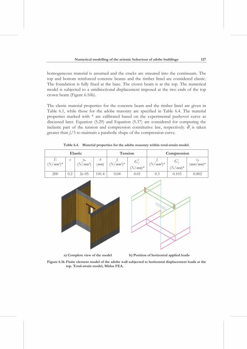
In this part the adobe wall tested by Blondet et al. [2005] is modelled using a continuum approach. A plane stress finite element model is created in Midas FEA using 4-node rectangular shell elements (Figure 6.16a) and considering drilling DOFs and transverse shear deformation. The size of the mesh is usually kept at 100 x 100 mm, which is related to a characteristic length dimension h= 141.4 mm, obtained from the square root of the area of the shell element [Bažant and Oh 1983]. The thickness of the shell is 300 mm. The adobe masonry includes the adobe bricks and the mud mortar joints; in this case, a
Numerical modelling of the seismic behaviour of adobe buildings
127
homogeneous material is assumed and the cracks are smeared into the continuum. The top and bottom reinforced concrete beams and the timber lintel are considered elastic. The foundation is fully fixed at the base. The crown beam is at the top. The numerical model is subjected to a unidirectional displacement imposed at the two ends of the top crown beam (Figure 6.16b).
The elastic material properties for the concrete beam and the timber lintel are given in Table 6.1, while those for the adobe masonry are specified in Table 6.4. The material properties marked with * are calibrated based on the experimental pushover curve as discussed later. Equation (5.29) and Equation (5.37) are considered for computing the inelastic part of the tension and compression constitutive law, respectively. i is taken greater than fc/3 to maintain a parabolic shape of the compression curve.
Table 6.4. Material properties for the adobe masonry within total-strain model.
Elastic Tension Compression
E (N/mm2)*
m (N/mm3)
h (mm)
ft (N/mm2)*
IfG
(N/mm)*
fc (N/mm2)*
cfG
(N/mm)*
p (mm/mm)*
200 0.2 2e-05 141.4 0.04 0.01 0.3 0.103 0.002
a) Complete view of the model b) Position of horizontal applied loads
Figure 6.16. Finite element model of the adobe wall subjected to horizontal displacement loads at the top. Total-strain model, Midas FEA.

Sabino Nicola Tarque Ruíz
128
6.3.1 Calibration of material properties
The first parameter that was calibrated is the elasticity modulus E of the adobe masonry. According to section 3.2.3.1 and 3.7, the E value can be considered between 200 and 220 MPa. Besides, [Blondet and Vargas 1978] suggests to use E= 170 MPa; however, this value seems to be too conservative. In this work E= 200 MPa has been considered for all the numerical analyses since it yields a good agreement between the numerical and experimental curves. Figure 6.17 shows the variation of the in-plane response of the adobe wall due to the variation of elasticity modulus. The other, elastic and inelastic, material properties used were the ones specified in Table 6.4.
0
5
10
15
20
25
30
35
40
45
0 2 4 6 8 10
Displacement (mm)
Forc
e (k
N)
ExperimentalE= 250 MPaE= 220 MPaE= 200 MPaE= 150 MPa
Figure 6.17. Comparison of the pushover curves in models with different E. Total-strain model.
The next parameter that was calibrated was the tensile strength ft of the masonry, which can be roughly assumed around 10% of the compression strength fc. The tensile fracture energy I
fG is maintained in all cases as 0.01 N/mm (Figure 6.18).
0
0.01
0.02
0.03
0.04
0.05
0.06
0.07
0 0.2 0.4 0.6 0.8 1
Crack displacement (mm)
Tens
ile s
tren
gth
(MPa
)
ft= 0.02 MPaft= 0.04 MPaft= 0.06 MPa
Figure 6.18. Variation of tensile strength for total-strain model, constant I
fG = 0.01 N/mm, h =
141.4 mm.
Numerical modelling of the seismic behaviour of adobe buildings
129
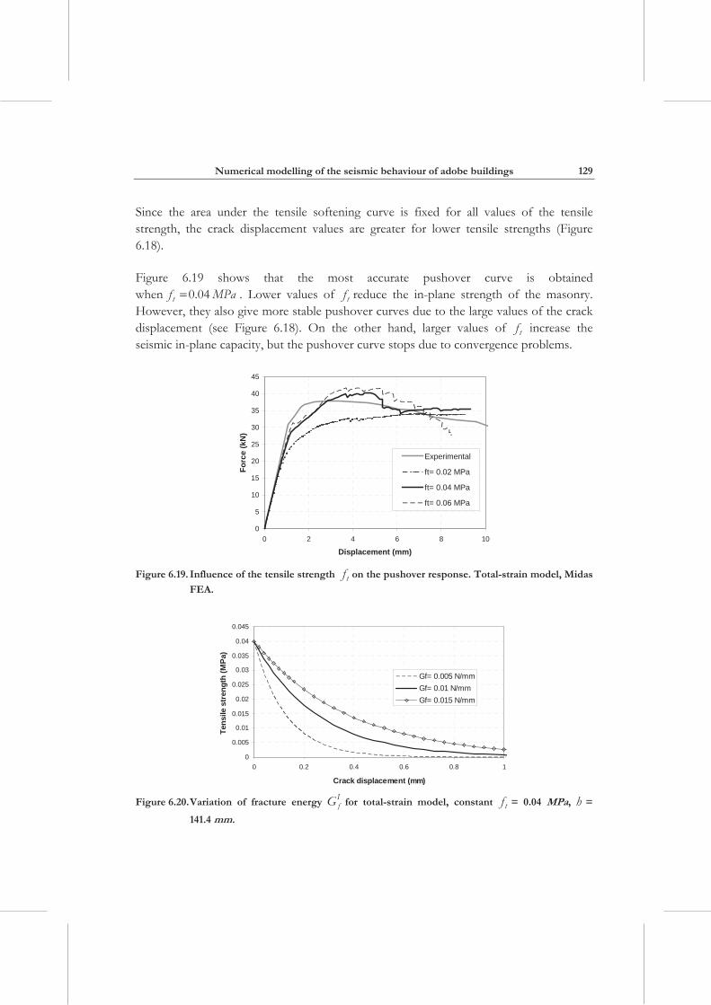
Since the area under the tensile softening curve is fixed for all values of the tensile strength, the crack displacement values are greater for lower tensile strengths (Figure 6.18).
Figure 6.19 shows that the most accurate pushover curve is obtained when tf MPa0.04 . Lower values of tf reduce the in-plane strength of the masonry. However, they also give more stable pushover curves due to the large values of the crack displacement (see Figure 6.18). On the other hand, larger values of tf increase the seismic in-plane capacity, but the pushover curve stops due to convergence problems.
0
5
10
15
20
25
30
35
40
45
0 2 4 6 8 10
Displacement (mm)
Forc
e (k
N)
Experimental
ft= 0.02 MPa
ft= 0.04 MPa
ft= 0.06 MPa
Figure 6.19. Influence of the tensile strength tf on the pushover response. Total-strain model, Midas
FEA.
0
0.005
0.01
0.015
0.02
0.025
0.03
0.035
0.04
0.045
0 0.2 0.4 0.6 0.8 1
Crack displacement (mm)
Tens
ile s
tren
gth
(MPa
)
Gf= 0.005 N/mmGf= 0.01 N/mmGf= 0.015 N/mm
Figure 6.20. Variation of fracture energy I
fG for total-strain model, constant tf = 0.04 MPa, h =
141.4 mm.
Sabino Nicola Tarque Ruíz
130
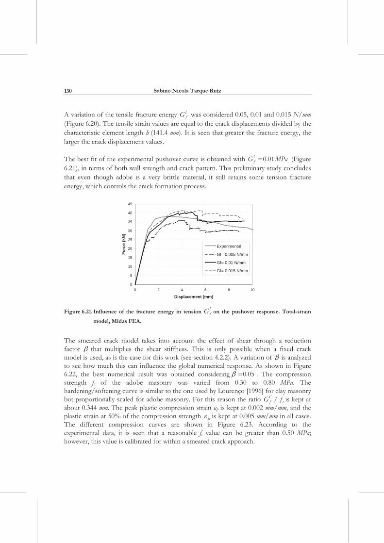
A variation of the tensile fracture energy IfG was considered 0.05, 0.01 and 0.015 N/mm
(Figure 6.20). The tensile strain values are equal to the crack displacements divided by the characteristic element length h (141.4 mm). It is seen that greater the fracture energy, the larger the crack displacement values.
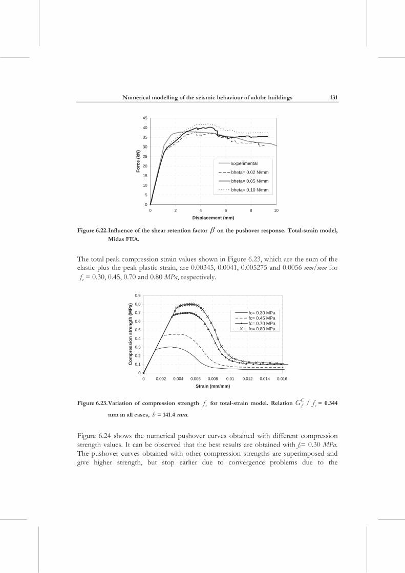
The best fit of the experimental pushover curve is obtained with IfG MPa0.01 (Figure
6.21), in terms of both wall strength and crack pattern. This preliminary study concludes that even though adobe is a very brittle material, it still retains some tension fracture energy, which controls the crack formation process.
0
5
10
15
20
25
30
35
40
45
0 2 4 6 8 10
Displacement (mm)
Forc
e (k
N)
Experimental
Gf= 0.005 N/mm
Gf= 0.01 N/mm
Gf= 0.015 N/mm
Figure 6.21. Influence of the fracture energy in tension IfG on the pushover response. Total-strain
model, Midas FEA.
The smeared crack model takes into account the effect of shear through a reduction factor that multiplies the shear stiffness. This is only possible when a fixed crack model is used, as is the case for this work (see section 4.2.2). A variation of is analyzed to see how much this can influence the global numerical response. As shown in Figure 6.22, the best numerical result was obtained considering 0.05 . The compression strength fc of the adobe masonry was varied from 0.30 to 0.80 MPa. The hardening/softening curve is similar to the one used by Lourenço [1996] for clay masonry but proportionally scaled for adobe masonry. For this reason the ratio C
f cG f/ is kept at about 0.344 mm. The peak plastic compression strain p is kept at 0.002 mm/mm, and the plastic strain at 50% of the compression strength m is kept at 0.005 mm/mm in all cases. The different compression curves are shown in Figure 6.23. According to the experimental data, it is seen that a reasonable fc value can be greater than 0.50 MPa; however, this value is calibrated for within a smeared crack approach.
Numerical modelling of the seismic behaviour of adobe buildings
131
0
5
10
15
20
25
30
35
40
45
0 2 4 6 8 10
Displacement (mm)
Forc
e (k
N)
Experimental
bheta= 0.02 N/mm
bheta= 0.05 N/mm
bheta= 0.10 N/mm
Figure 6.22. Influence of the shear retention factor on the pushover response. Total-strain model,
Midas FEA.
The total peak compression strain values shown in Figure 6.23, which are the sum of the elastic plus the peak plastic strain, are 0.00345, 0.0041, 0.005275 and 0.0056 mm/mm for
cf = 0.30, 0.45, 0.70 and 0.80 MPa, respectively.
0
0.1
0.2
0.3
0.4
0.5
0.6
0.7
0.8
0.9
0 0.002 0.004 0.006 0.008 0.01 0.012 0.014 0.016
Strain (mm/mm)
Com
pres
sion
str
engt
h (M
Pa)
fc= 0.30 MPafc= 0.45 MPafc= 0.70 MPafc= 0.80 MPa
Figure 6.23. Variation of compression strength cf for total-strain model. Relation Cf cG f/ = 0.344
mm in all cases, h = 141.4 mm.
Figure 6.24 shows the numerical pushover curves obtained with different compression strength values. It can be observed that the best results are obtained with fc= 0.30 MPa. The pushover curves obtained with other compression strengths are superimposed and give higher strength, but stop earlier due to convergence problems due to the

Sabino Nicola Tarque Ruíz
132
concentration of compression stress at the right top window corner. If convergence is reached, so the pushover curve will down and continues closes to the experimental curve.
0
5
10
15
20
25
30
35
40
45
0 2 4 6 8 10
Displacement (mm)
Forc
e (k
N)
Experimentalfc= 0.45 MPafc= 0.30 MPafc= 0.70 MPafc= 0.80 MPa
Figure 6.24. Influence of the compression strength cf on the pushover response. Total-strain model,
Midas FEA.
6.3.2 Results of the pushover analysis considering a total-strain model
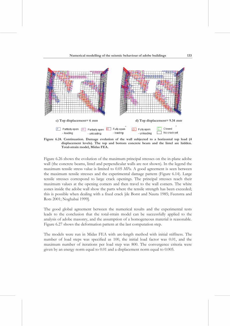
Figure 6.25 shows the sequence of damage obtained with the parameters specified in Table 6.4. Only the adobe walls are shown here; the ring concrete beams and the lintel are hidden. The maximum top displacement reached was around 9.34 mm. Similar to the experimental response (Figure 6.13), the numerical results show a diagonal crack forming from the corners of the opening. Horizontal cracks are also detected in the perpendicular walls.
a) Top displacement= 1 mm b) Top displacement= 4 mm
Figure 6.25. Damage evolution of the wall subjected to a horizontal top load (4 displacement levels). The top and bottom concrete beam and the lintel are hidden. Total-strain model, Midas FEA.
Numerical modelling of the seismic behaviour of adobe buildings
133
c) Top displacement= 6 mm d) Top displacement= 9.34 mm
Figure 6.24. Continuation. Damage evolution of the wall subjected to a horizontal top load (4
displacement levels). The top and bottom concrete beam and the lintel are hidden. Total-strain model, Midas FEA.
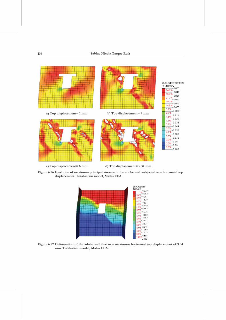
Figure 6.26 shows the evolution of the maximum principal stresses on the in-plane adobe wall (the concrete beams, lintel and perpendicular walls are not shown). In the legend the maximum tensile stress value is limited to 0.05 MPa. A good agreement is seen between the maximum tensile stresses and the experimental damage pattern (Figure 6.14). Large tensile stresses correspond to large crack openings. The principal stresses reach their maximum values at the opening corners and then travel to the wall corners. The white zones inside the adobe wall show the parts where the tensile strength has been exceeded; this is possible when dealing with a fixed crack [de Borst and Nauta 1985; Feenstra and Rots 2001; Noghabai 1999].
The good global agreement between the numerical results and the experimental tests leads to the conclusion that the total-strain model can be successfully applied to the analysis of adobe masonry, and the assumption of a homogeneous material is reasonable. Figure 6.27 shows the deformation pattern at the last computation step.
The models were run in Midas FEA with arc-length method with initial stiffness. The number of load steps was specified as 100, the initial load factor was 0.01, and the maximum number of iterations per load step was 800. The convergence criteria were given by an energy norm equal to 0.01 and a displacement norm equal to 0.005.
Sabino Nicola Tarque Ruíz
134
a) Top displacement= 1 mm b) Top displacement= 4 mm
c) Top displacement= 6 mm d) Top displacement= 9.34 mm
Figure 6.26. Evolution of maximum principal stresses in the adobe wall subjected to a horizontal top displacement. Total-strain model, Midas FEA.
Figure 6.27. Deformation of the adobe wall due to a maximum horizontal top displacement of 9.34
mm. Total-strain model, Midas FEA.
Numerical modelling of the seismic behaviour of adobe buildings
135
6.4 CONCRETE DAMAGED PLASTICITY: MODELLING THE PUSHOVER RESPONSE.
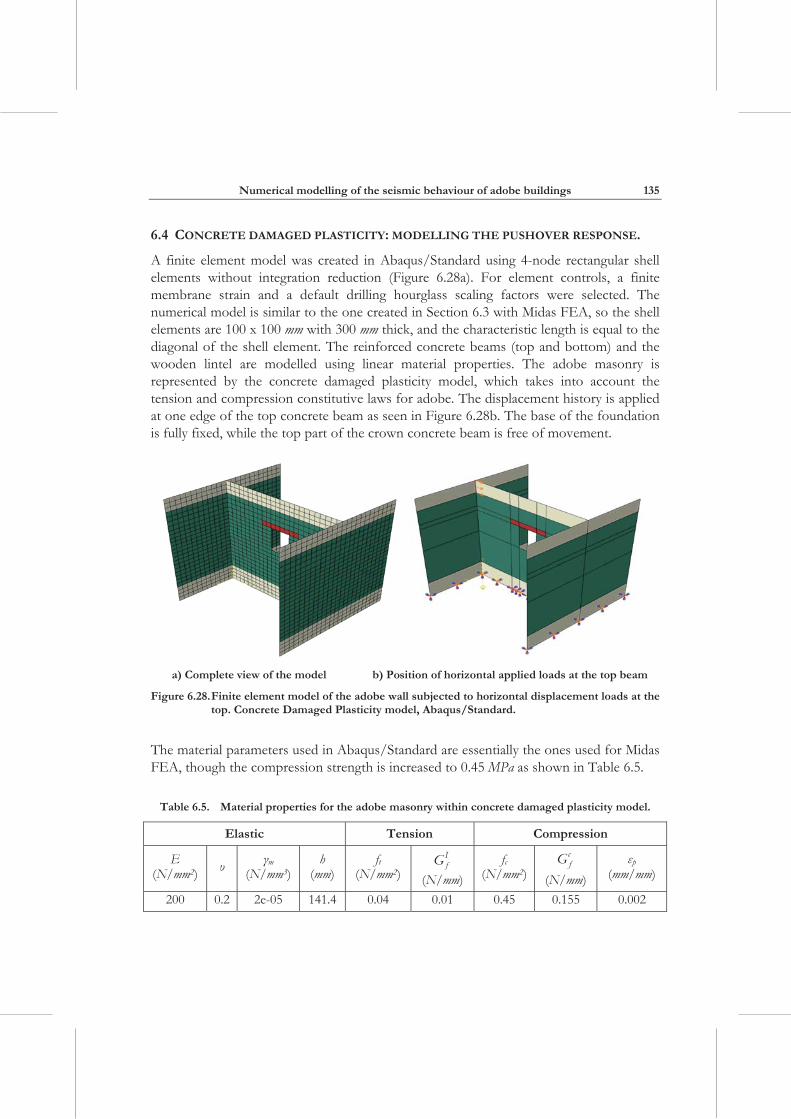
A finite element model was created in Abaqus/Standard using 4-node rectangular shell elements without integration reduction (Figure 6.28a). For element controls, a finite membrane strain and a default drilling hourglass scaling factors were selected. The numerical model is similar to the one created in Section 6.3 with Midas FEA, so the shell elements are 100 x 100 mm with 300 mm thick, and the characteristic length is equal to the diagonal of the shell element. The reinforced concrete beams (top and bottom) and the wooden lintel are modelled using linear material properties. The adobe masonry is represented by the concrete damaged plasticity model, which takes into account the tension and compression constitutive laws for adobe. The displacement history is applied at one edge of the top concrete beam as seen in Figure 6.28b. The base of the foundation is fully fixed, while the top part of the crown concrete beam is free of movement.
a) Complete view of the model b) Position of horizontal applied loads at the top beam
Figure 6.28. Finite element model of the adobe wall subjected to horizontal displacement loads at the top. Concrete Damaged Plasticity model, Abaqus/Standard.
The material parameters used in Abaqus/Standard are essentially the ones used for Midas FEA, though the compression strength is increased to 0.45 MPa as shown in Table 6.5.
Table 6.5. Material properties for the adobe masonry within concrete damaged plasticity model.
Elastic Tension Compression
E (N/mm2) m
(N/mm3) h
(mm) ft
(N/mm2) IfG
(N/mm) fc
(N/mm2)cfG
(N/mm) p
(mm/mm)
200 0.2 2e-05 141.4 0.04 0.01 0.45 0.155 0.002
Sabino Nicola Tarque Ruíz
136
The following default additional parameters are required for the concrete damaged plasticity model: dilatation angle= 1, eccentricity= 0.1, ratio of initial equibiaxial compressive yield stress to initial uniaxial compressive yield stress= 1.16, k parameter related to yield surface= 2/3, and null viscosity parameter.
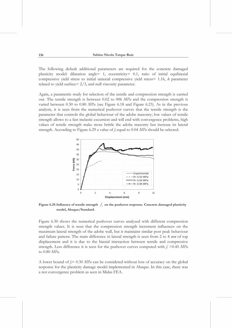
Again, a parametric study for selection of the tensile and compression strength is carried out. The tensile strength is between 0.02 to 006 MPa and the compression strength is varied between 0.30 to 0.80 MPa (see Figure 6.18 and Figure 6.23). As in the previous analysis, it is seen from the numerical pushover curves that the tensile strength is the parameter that controls the global behaviour of the adobe masonry; low values of tensile strength allows to a fast inelastic excursion and will end with convergence problems, high values of tensile strength make more brittle the adobe masonry but increase its lateral strength. According to Figure 6.29 a value of ft equal to 0.04 MPa should be selected.
0
5
10
15
20
25
30
35
40
45
50
0 2 4 6 8 10
Displacement (mm)
Forc
e (k
N)
Experimentalft= 0.02 MPaft= 0.04 MPaft= 0.06 MPa
Figure 6.29. Influence of tensile strength tf on the pushover response. Concrete damaged plasticity
model, Abaqus/Standard.
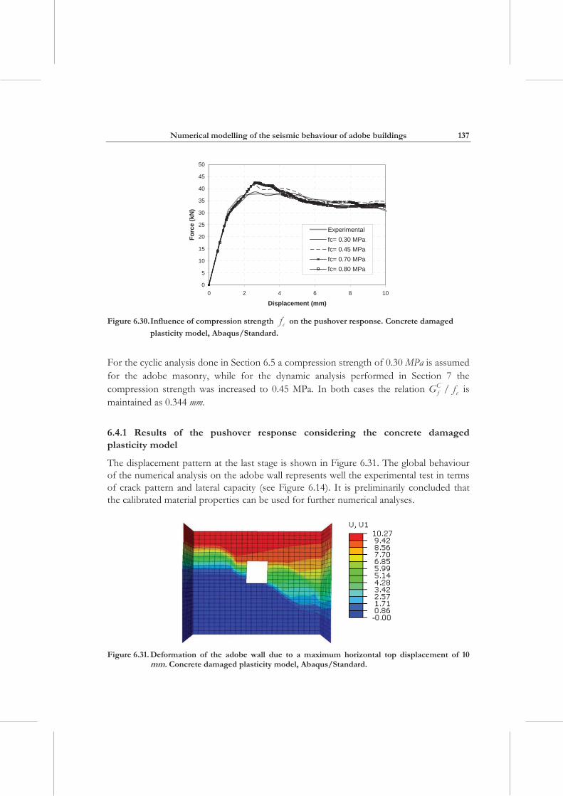
Figure 6.30 shows the numerical pushover curves analyzed with different compression strength values. It is seen that the compression strength increment influences on the maximum lateral strength of the adobe wall, but it maintains similar post peak behaviour and failure pattern. The main difference in lateral strength is seen from 2 to 4 mm of top displacement and it is due to the biaxial interaction between tensile and compressive strength. Less difference it is seen for the pushover curves computed with fc =0.45 MPa to 0.80 MPa.
A lower bound of fc= 0.30 MPa can be considered without loss of accuracy on the global response for the plasticity damage model implemented in Abaqus. In this case, there was a not convergence problem as seen in Midas FEA.
Numerical modelling of the seismic behaviour of adobe buildings
137
0
5
10
15
20
25
30
35
40
45
50
0 2 4 6 8 10
Displacement (mm)
Forc
e (k
N)
Experimentalfc= 0.30 MPafc= 0.45 MPafc= 0.70 MPafc= 0.80 MPa
Figure 6.30. Influence of compression strength cf on the pushover response. Concrete damaged
plasticity model, Abaqus/Standard.
For the cyclic analysis done in Section 6.5 a compression strength of 0.30 MPa is assumed for the adobe masonry, while for the dynamic analysis performed in Section 7 the compression strength was increased to 0.45 MPa. In both cases the relation C
f cG f/ is maintained as 0.344 mm.
6.4.1 Results of the pushover response considering the concrete damaged plasticity model
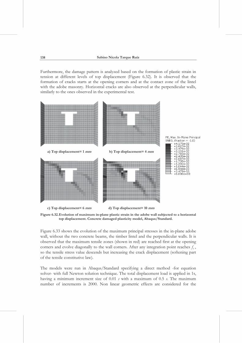
The displacement pattern at the last stage is shown in Figure 6.31. The global behaviour of the numerical analysis on the adobe wall represents well the experimental test in terms of crack pattern and lateral capacity (see Figure 6.14). It is preliminarily concluded that the calibrated material properties can be used for further numerical analyses.
Figure 6.31. Deformation of the adobe wall due to a maximum horizontal top displacement of 10
mm. Concrete damaged plasticity model, Abaqus/Standard.
Sabino Nicola Tarque Ruíz
138
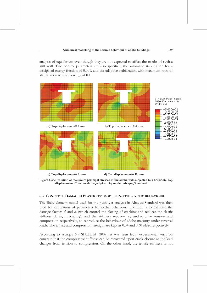
Furthermore, the damage pattern is analyzed based on the formation of plastic strain in tension at different levels of top displacement (Figure 6.32). It is observed that the formation of cracks starts at the opening corners and at the contact zone of the lintel with the adobe masonry. Horizontal cracks are also observed at the perpendicular walls, similarly to the ones observed in the experimental test.
a) Top displacement= 1 mm b) Top displacement= 4 mm
c) Top displacement= 6 mm d) Top displacement= 10 mm
Figure 6.32. Evolution of maximum in-plane plastic strain in the adobe wall subjected to a horizontal top displacement. Concrete damaged plasticity model, Abaqus/Standard.
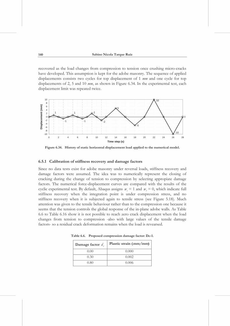
Figure 6.33 shows the evolution of the maximum principal stresses in the in-plane adobe wall, without the two concrete beams, the timber lintel and the perpendicular walls. It is observed that the maximum tensile zones (shown in red) are reached first at the opening corners and evolve diagonally to the wall corners. After any integration point reaches tf , so the tensile stress value descends but increasing the crack displacement (softening part of the tensile constitutive law).
The models were run in Abaqus/Standard specifying a direct method -for equation solver- with full Newton solution technique. The total displacement load is applied in 1s, having a minimum increment size of 0.01 s with a maximum of 0.5 s. The maximum number of increments is 2000. Non linear geometric effects are considered for the
Numerical modelling of the seismic behaviour of adobe buildings
139
analysis of equilibrium even though they are not expected to affect the results of such a stiff wall. Two control parameters are also specified, the automatic stabilization for a dissipated energy fraction of 0.001, and the adaptive stabilization with maximum ratio of stabilization to strain energy of 0.1.
a) Top displacement= 1 mm b) Top displacement= 4 mm
c) Top displacement= 6 mm d) Top displacement= 10 mm
Figure 6.33. Evolution of maximum principal stresses in the adobe wall subjected to a horizontal top displacement. Concrete damaged plasticity model, Abaqus/Standard.
6.5 CONCRETE DAMAGED PLASTICITY: MODELLING THE CYCLIC BEHAVIOUR
The finite element model used for the pushover analysis in Abaqus/Standard was then used for calibration of parameters for cyclic behaviour. The idea is to calibrate the damage factors dt and dc (which control the closing of cracking and reduces the elastic stiffness during unloading), and the stiffness recovery tw and cw , for tension and compression respectively, to reproduce the behaviour of adobe masonry under reversal loads. The tensile and compression strength are kept as 0.04 and 0.30 MPa, respectively.
According to Abaqus 6.9 SIMULIA [2009], it was seen from experimental tests on concrete that the compressive stiffness can be recovered upon crack closure as the load changes from tension to compression. On the other hand, the tensile stiffness is not
Sabino Nicola Tarque Ruíz
140
recovered as the load changes from compression to tension once crushing micro-cracks have developed. This assumption is kept for the adobe masonry. The sequence of applied displacements consists two cycles for top displacement of 1 mm and one cycle for top displacements of 2, 5 and 10 mm, as shown in Figure 6.34. In the experimental test, each displacement limit was repeated twice.
2
-2
0
1
-1
1
-1
-10
10
-5
5
-10-8-6-4-202468
10
0 2 4 6 8 10 12 14 16 18 20 22 24 26 28
Time step (s)
Dis
plac
emen
t (m
m)
Figure 6.34. History of static horizontal displacement load applied to the numerical model.
6.5.1 Calibration of stiffness recovery and damage factors
Since no data tests exist for adobe masonry under reversal loads, stiffness recovery and damage factors were assumed. The idea was to numerically represent the closing of cracking during the change of tension to compression by selecting appropiate damage factors. The numerical force-displacement curves are compared with the results of the cyclic experimental test. By default, Abaqus assigns cw = 1 and tw = 0, which indicate full stiffness recovery when the integration point is under compression stress, and no stiffness recovery when it is subjected again to tensile stress (see Figure 5.18). Much attention was given to the tensile behaviour rather than to the compression one because it seems that the tension controls the global response of the in-plane adobe walls. As Table 6.6 to Table 6.16 show it is not possible to reach zero crack displacement when the load changes from tension to compression -also with large values of the tensile damage factors- so a residual crack deformation remains when the load is revearsed.
Table 6.6. Proposed compression damage factor: Dc-1.
Damage factor cd Plastic strain (mm/mm)
0.00 0.000 0.30 0.002 0.80 0.006
Numerical modelling of the seismic behaviour of adobe buildings
141
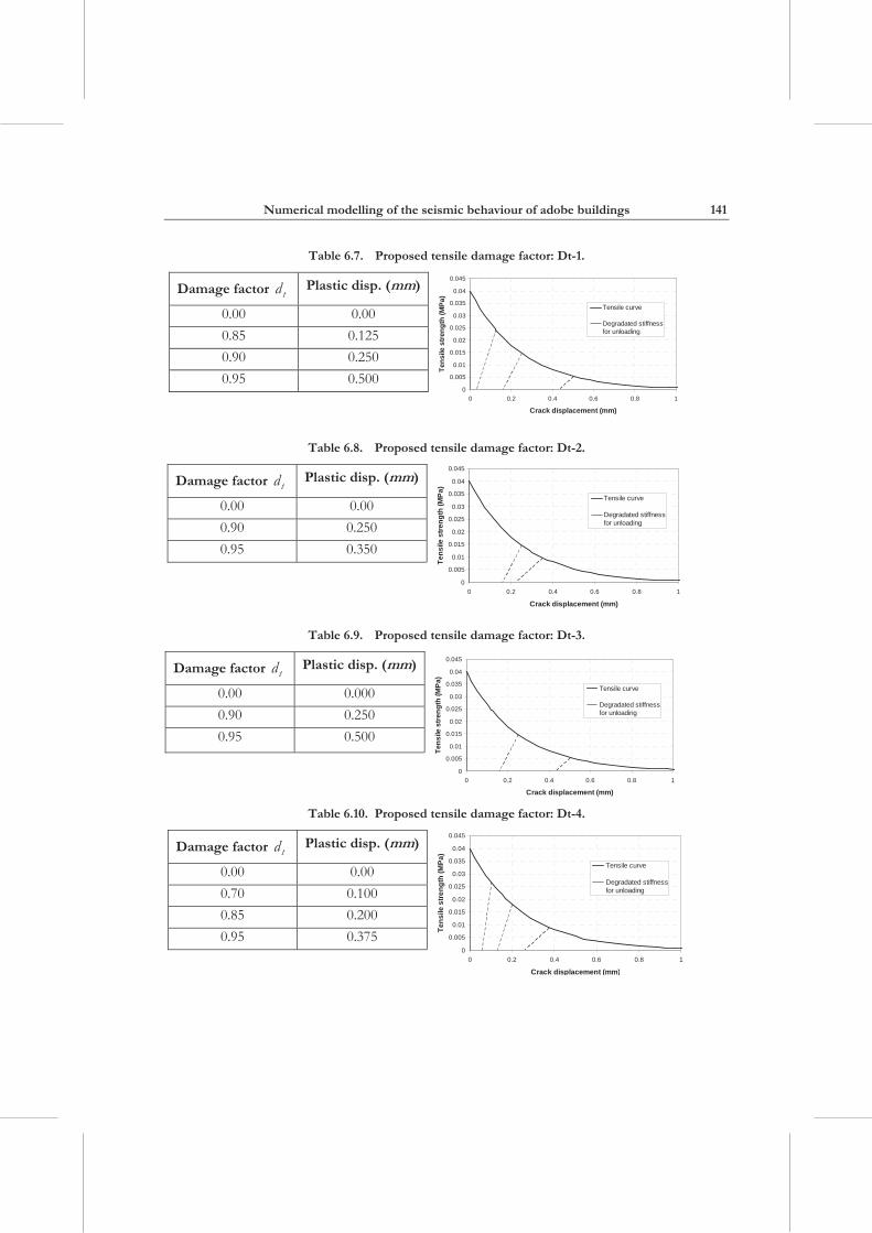
Table 6.7. Proposed tensile damage factor: Dt-1.
Damage factor td Plastic disp. (mm)
0.00 0.00 0.85 0.125 0.90 0.250 0.95 0.500
0
0.005
0.01
0.015
0.02
0.025
0.03
0.035
0.04
0.045
0 0.2 0.4 0.6 0.8 1
Crack displacement (mm)
Tens
ile s
treng
th (M
Pa)
Tensile curve
Degradated stiffnessfor unloading
Table 6.8. Proposed tensile damage factor: Dt-2.
Damage factor td Plastic disp. (mm)
0.00 0.00 0.90 0.250 0.95 0.350
0
0.005
0.01
0.015
0.02
0.025
0.03
0.035
0.04
0.045
0 0.2 0.4 0.6 0.8 1
Crack displacement (mm)
Tens
ile s
treng
th (M
Pa)
Tensile curve
Degradated stiffnessfor unloading
Table 6.9. Proposed tensile damage factor: Dt-3.
Damage factor td Plastic disp. (mm)
0.00 0.000 0.90 0.250 0.95 0.500
0
0.005
0.01
0.015
0.02
0.025
0.03
0.035
0.04
0.045
0 0.2 0.4 0.6 0.8 1
Crack displacement (mm)
Tens
ile s
treng
th (M
Pa)
Tensile curve
Degradated stiffnessfor unloading
Table 6.10. Proposed tensile damage factor: Dt-4.
Damage factor td Plastic disp. (mm)
0.00 0.00 0.70 0.100 0.85 0.200 0.95 0.375
0
0.005
0.01
0.015
0.02
0.025
0.03
0.035
0.04
0.045
0 0.2 0.4 0.6 0.8 1
Crack displacement (mm)
Tens
ile s
treng
th (M
Pa)
Tensile curve
Degradated stiffnessfor unloading
Sabino Nicola Tarque Ruíz
142
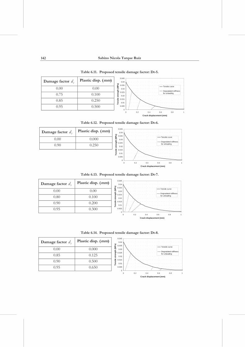
Table 6.11. Proposed tensile damage factor: Dt-5.
Damage factor td Plastic disp. (mm)
0.00 0.00 0.75 0.100 0.85 0.250 0.95 0.500
0
0.005
0.01
0.015
0.02
0.025
0.03
0.035
0.04
0.045
0 0.2 0.4 0.6 0.8 1
Crack displacement (mm)Te
nsile
stre
ngth
(MPa
)
Tensile curve
Degradated stiffnessfor unloading
Table 6.12. Proposed tensile damage factor: Dt-6.
Damage factor td Plastic disp. (mm)
0.00 0.000 0.90 0.250
0
0.005
0.01
0.015
0.02
0.025
0.03
0.035
0.04
0.045
0 0.2 0.4 0.6 0.8 1
Crack displacement (mm)
Tens
ile s
treng
th (M
Pa)
Tensile curve
Degradated stiffnessfor unloading
Table 6.13. Proposed tensile damage factor: Dt-7.
Damage factor td Plastic disp. (mm)
0.00 0.00 0.80 0.100 0.90 0.200 0.95 0.300
0
0.005
0.01
0.015
0.02
0.025
0.03
0.035
0.04
0.045
0 0.2 0.4 0.6 0.8 1
Crack displacement (mm)
Tens
ile s
treng
th (M
Pa)
Tensile curve
Degradated stiffnessfor unloading
Table 6.14. Proposed tensile damage factor: Dt-8.
Damage factor td Plastic disp. (mm)
0.00 0.000 0.85 0.125 0.90 0.500 0.95 0.650
0
0.005
0.01
0.015
0.02
0.025
0.03
0.035
0.04
0.045
0 0.2 0.4 0.6 0.8 1
Crack displacement (mm)
Tens
ile s
treng
th (M
Pa)
Tensile curve
Degradated stiffnessfor unloading
Numerical modelling of the seismic behaviour of adobe buildings
143
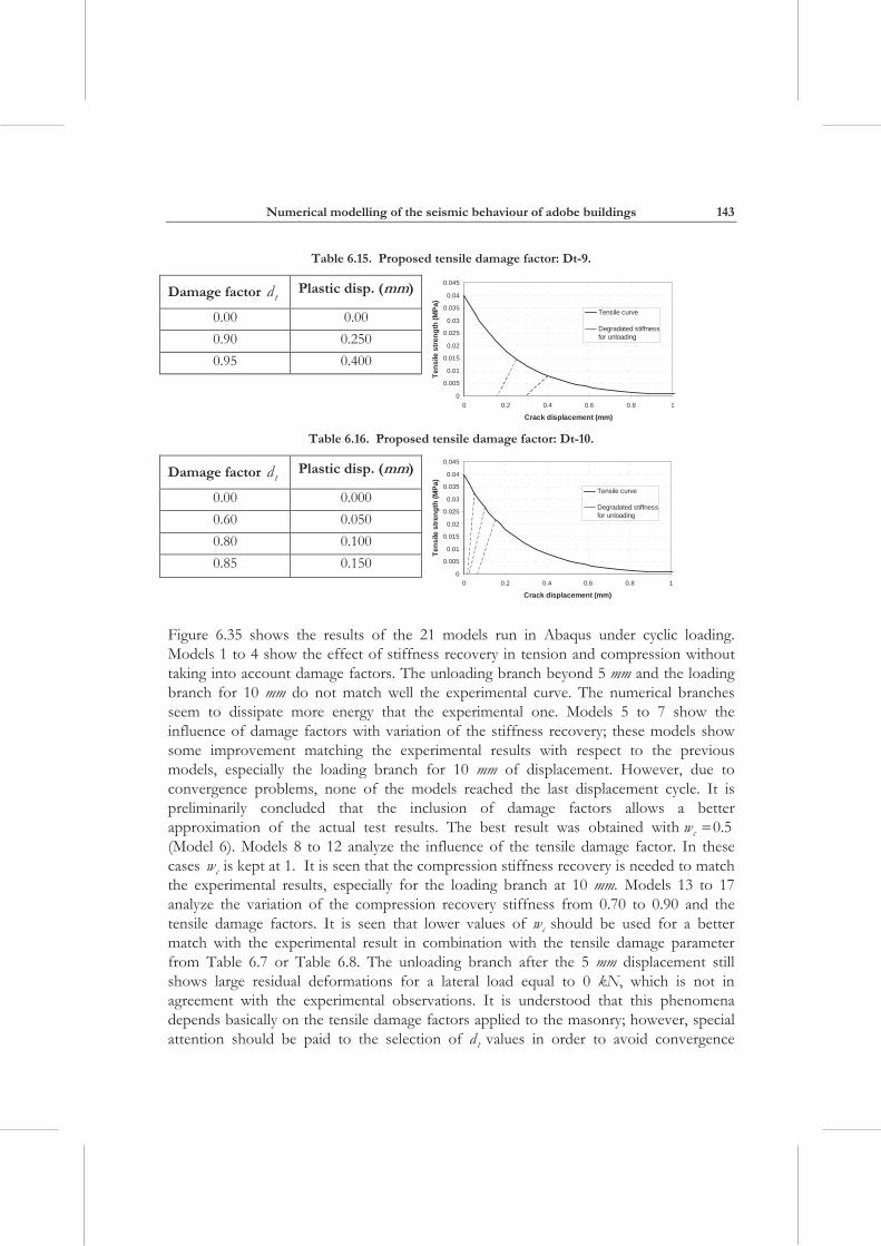
Table 6.15. Proposed tensile damage factor: Dt-9.
Damage factor td Plastic disp. (mm)
0.00 0.00 0.90 0.250 0.95 0.400
0
0.005
0.01
0.015
0.02
0.025
0.03
0.035
0.04
0.045
0 0.2 0.4 0.6 0.8 1
Crack displacement (mm)
Tens
ile s
treng
th (M
Pa)
Tensile curve
Degradated stiffnessfor unloading
Table 6.16. Proposed tensile damage factor: Dt-10.
Damage factor td Plastic disp. (mm)
0.00 0.000 0.60 0.050 0.80 0.100 0.85 0.150
0
0.005
0.01
0.015
0.02
0.025
0.03
0.035
0.04
0.045
0 0.2 0.4 0.6 0.8 1
Crack displacement (mm)
Tens
ile s
treng
th (M
Pa)
Tensile curve
Degradated stiffnessfor unloading
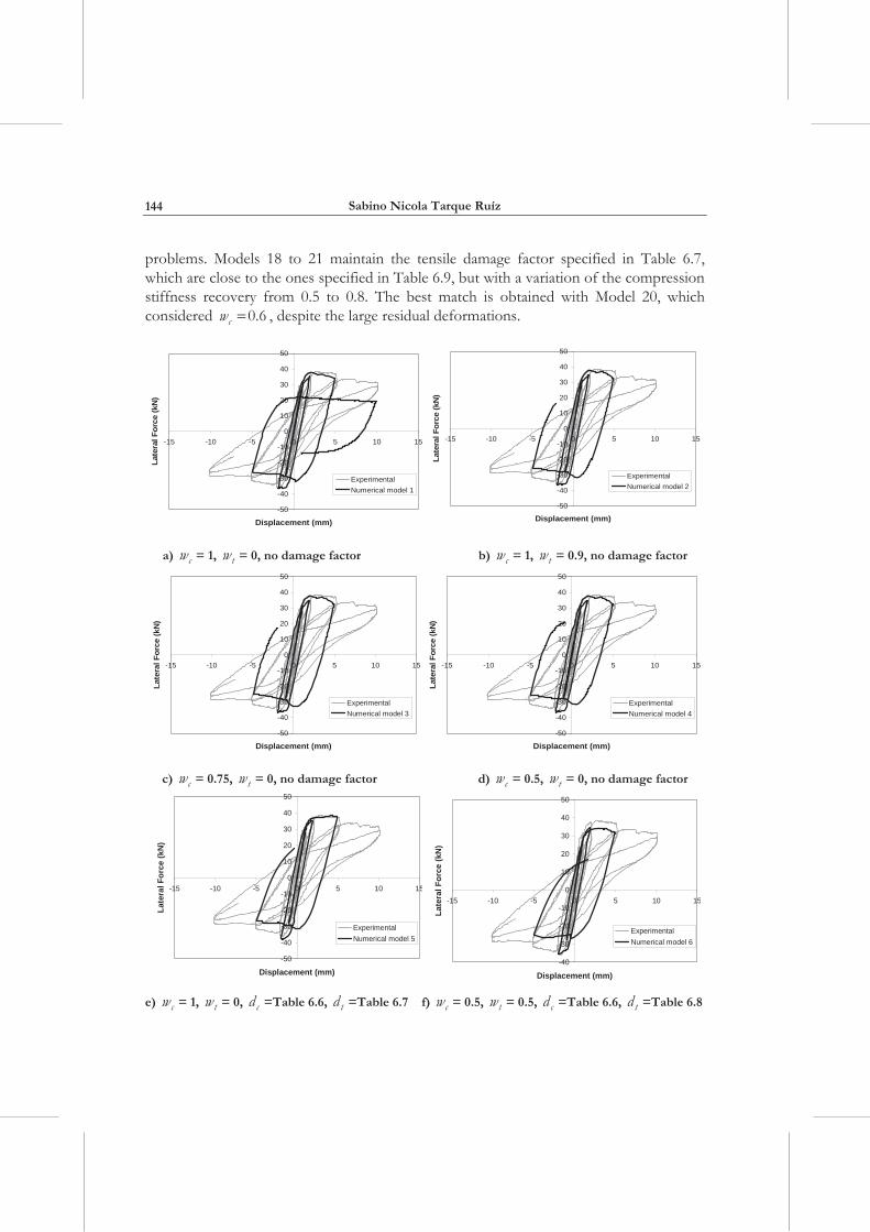
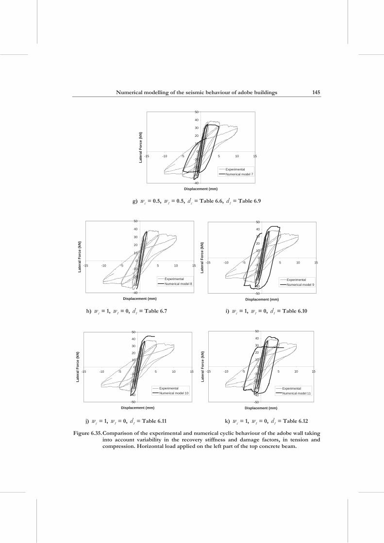
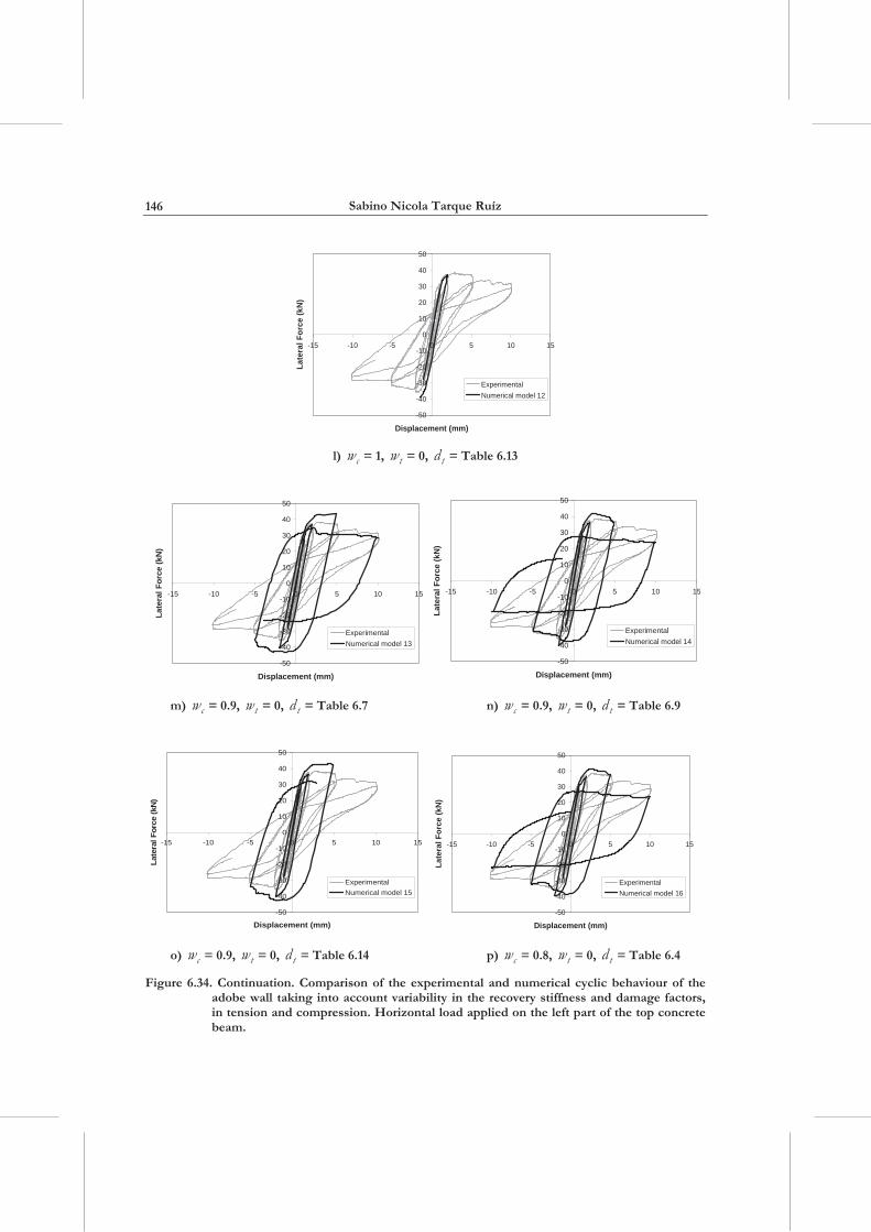
Figure 6.35 shows the results of the 21 models run in Abaqus under cyclic loading. Models 1 to 4 show the effect of stiffness recovery in tension and compression without taking into account damage factors. The unloading branch beyond 5 mm and the loading branch for 10 mm do not match well the experimental curve. The numerical branches seem to dissipate more energy that the experimental one. Models 5 to 7 show the influence of damage factors with variation of the stiffness recovery; these models show some improvement matching the experimental results with respect to the previous models, especially the loading branch for 10 mm of displacement. However, due to convergence problems, none of the models reached the last displacement cycle. It is preliminarily concluded that the inclusion of damage factors allows a better approximation of the actual test results. The best result was obtained with cw 0.5 (Model 6). Models 8 to 12 analyze the influence of the tensile damage factor. In these cases cw is kept at 1. It is seen that the compression stiffness recovery is needed to match the experimental results, especially for the loading branch at 10 mm. Models 13 to 17 analyze the variation of the compression recovery stiffness from 0.70 to 0.90 and the tensile damage factors. It is seen that lower values of cw should be used for a better match with the experimental result in combination with the tensile damage parameter from Table 6.7 or Table 6.8. The unloading branch after the 5 mm displacement still shows large residual deformations for a lateral load equal to 0 kN, which is not in agreement with the experimental observations. It is understood that this phenomena depends basically on the tensile damage factors applied to the masonry; however, special attention should be paid to the selection of td values in order to avoid convergence
Sabino Nicola Tarque Ruíz
144
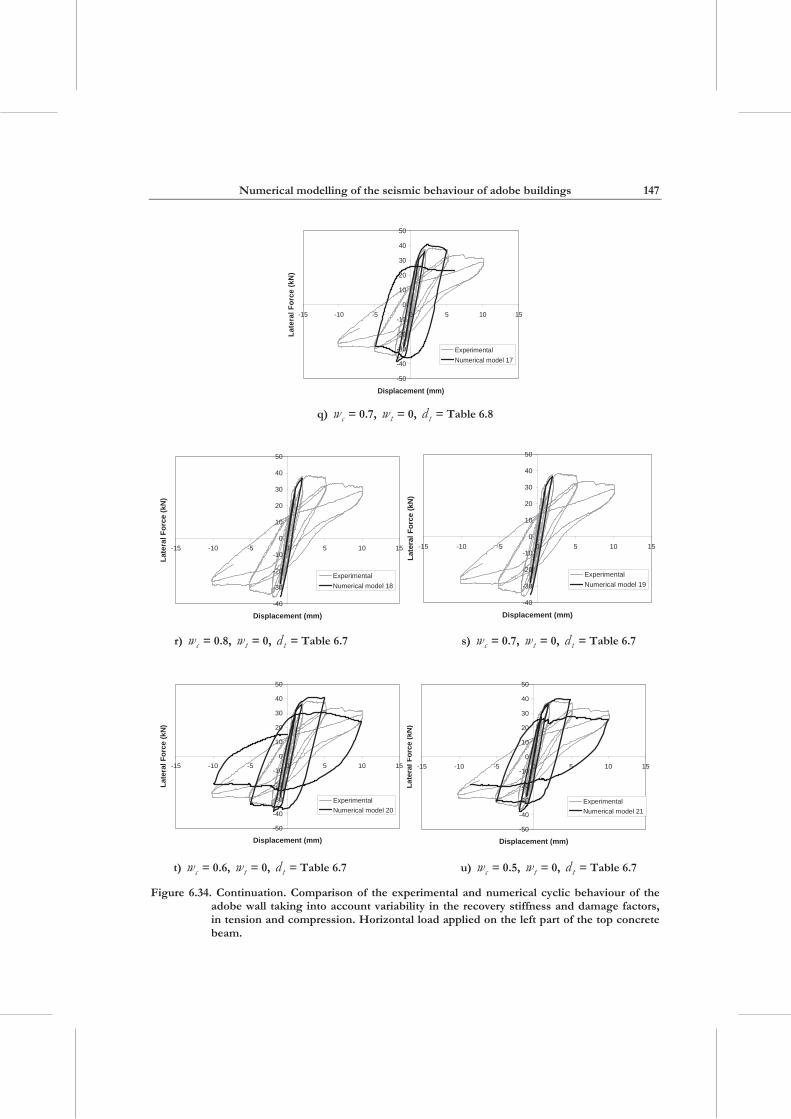
problems. Models 18 to 21 maintain the tensile damage factor specified in Table 6.7, which are close to the ones specified in Table 6.9, but with a variation of the compression stiffness recovery from 0.5 to 0.8. The best match is obtained with Model 20, which considered cw 0.6 , despite the large residual deformations.
-50
-40
-30
-20
-10
0
10
20
30
40
50
-15 -10 -5 0 5 10 15
Displacement (mm)
Late
ral F
orce
(kN
)
ExperimentalNumerical model 1
-50
-40
-30
-20
-10
0
10
20
30
40
50
-15 -10 -5 0 5 10 15
Displacement (mm)
Late
ral F
orce
(kN
)
ExperimentalNumerical model 2
a) cw = 1, tw = 0, no damage factor b) cw = 1, tw = 0.9, no damage factor
-50
-40
-30
-20
-10
0
10
20
30
40
50
-15 -10 -5 0 5 10 15
Displacement (mm)
Late
ral F
orce
(kN
)
ExperimentalNumerical model 3
-50
-40
-30
-20
-10
0
10
20
30
40
50
-15 -10 -5 0 5 10 15
Displacement (mm)
Late
ral F
orce
(kN
)
ExperimentalNumerical model 4
c) cw = 0.75, tw = 0, no damage factor d) cw = 0.5, tw = 0, no damage factor
-50
-40
-30
-20
-10
0
10
20
30
40
50
-15 -10 -5 0 5 10 15
Displacement (mm)
Late
ral F
orce
(kN
)
ExperimentalNumerical model 5
-40
-30
-20
-10
0
10
20
30
40
50
-15 -10 -5 0 5 10 15
Displacement (mm)
Late
ral F
orce
(kN
)
ExperimentalNumerical model 6
e) cw = 1, tw = 0, cd =Table 6.6, td =Table 6.7 f) cw = 0.5, tw = 0.5, cd =Table 6.6, td =Table 6.8
Numerical modelling of the seismic behaviour of adobe buildings
145
-40
-30
-20
-10
0
10
20
30
40
50
-15 -10 -5 0 5 10 15
Displacement (mm)
Late
ral F
orce
(kN
)
ExperimentalNumerical model 7
g) cw = 0.5, tw = 0.5, cd = Table 6.6, td = Table 6.9
-40
-30
-20
-10
0
10
20
30
40
50
-15 -10 -5 0 5 10 15
Displacement (mm)
Late
ral F
orce
(kN
)
ExperimentalNumerical model 8
-50
-40
-30
-20
-10
0
10
20
30
40
50
-15 -10 -5 0 5 10 15
Displacement (mm)
Late
ral F
orce
(kN
)
ExperimentalNumerical model 9
h) cw = 1, tw = 0, td = Table 6.7 i) cw = 1, tw = 0, td = Table 6.10
-50
-40
-30
-20
-10
0
10
20
30
40
50
-15 -10 -5 0 5 10 15
Displacement (mm)
Late
ral F
orce
(kN
)
ExperimentalNumerical model 10
-50
-40
-30
-20
-10
0
10
20
30
40
50
-15 -10 -5 0 5 10 15
Displacement (mm)
Late
ral F
orce
(kN
)
ExperimentalNumerical model 11
j) cw = 1, tw = 0, td = Table 6.11 k) cw = 1, tw = 0, td = Table 6.12
Figure 6.35. Comparison of the experimental and numerical cyclic behaviour of the adobe wall taking into account variability in the recovery stiffness and damage factors, in tension and compression. Horizontal load applied on the left part of the top concrete beam.
Sabino Nicola Tarque Ruíz
146
-50
-40
-30
-20
-10
0
10
20
30
40
50
-15 -10 -5 0 5 10 15
Displacement (mm)
Late
ral F
orce
(kN
)
ExperimentalNumerical model 12
l) cw = 1, tw = 0, td = Table 6.13
-50
-40
-30
-20
-10
0
10
20
30
40
50
-15 -10 -5 0 5 10 15
Displacement (mm)
Late
ral F
orce
(kN
)
ExperimentalNumerical model 13
-50
-40
-30
-20
-10
0
10
20
30
40
50
-15 -10 -5 0 5 10 15
Displacement (mm)
Late
ral F
orce
(kN
)
ExperimentalNumerical model 14
m) cw = 0.9, tw = 0, td = Table 6.7 n) cw = 0.9, tw = 0, td = Table 6.9
-50
-40
-30
-20
-10
0
10
20
30
40
50
-15 -10 -5 0 5 10 15
Displacement (mm)
Late
ral F
orce
(kN
)
ExperimentalNumerical model 15
-50
-40
-30
-20
-10
0
10
20
30
40
50
-15 -10 -5 0 5 10 15
Displacement (mm)
Late
ral F
orce
(kN
)
ExperimentalNumerical model 16
o) cw = 0.9, tw = 0, td = Table 6.14 p) cw = 0.8, tw = 0, td = Table 6.4
Figure 6.34. Continuation. Comparison of the experimental and numerical cyclic behaviour of the adobe wall taking into account variability in the recovery stiffness and damage factors, in tension and compression. Horizontal load applied on the left part of the top concrete beam.
Numerical modelling of the seismic behaviour of adobe buildings
147
-50
-40
-30
-20
-10
0
10
20
30
40
50
-15 -10 -5 0 5 10 15
Displacement (mm)
Late
ral F
orce
(kN
)
ExperimentalNumerical model 17
q) cw = 0.7, tw = 0, td = Table 6.8
-40
-30
-20
-10
0
10
20
30
40
50
-15 -10 -5 0 5 10 15
Displacement (mm)
Late
ral F
orce
(kN
)
ExperimentalNumerical model 18
-40
-30
-20
-10
0
10
20
30
40
50
-15 -10 -5 0 5 10 15
Displacement (mm)
Late
ral F
orce
(kN
)
ExperimentalNumerical model 19
r) cw = 0.8, tw = 0, td = Table 6.7 s) cw = 0.7, tw = 0, td = Table 6.7
-50
-40
-30
-20
-10
0
10
20
30
40
50
-15 -10 -5 0 5 10 15
Displacement (mm)
Late
ral F
orce
(kN
)
ExperimentalNumerical model 20
-50
-40
-30
-20
-10
0
10
20
30
40
50
-15 -10 -5 0 5 10 15
Displacement (mm)
Late
ralF
orce
(kN
)
ExperimentalNumerical model 21
t) cw = 0.6, tw = 0, td = Table 6.7 u) cw = 0.5, tw = 0, td = Table 6.7
Figure 6.34. Continuation. Comparison of the experimental and numerical cyclic behaviour of the adobe wall taking into account variability in the recovery stiffness and damage factors, in tension and compression. Horizontal load applied on the left part of the top concrete beam.
Sabino Nicola Tarque Ruíz
148
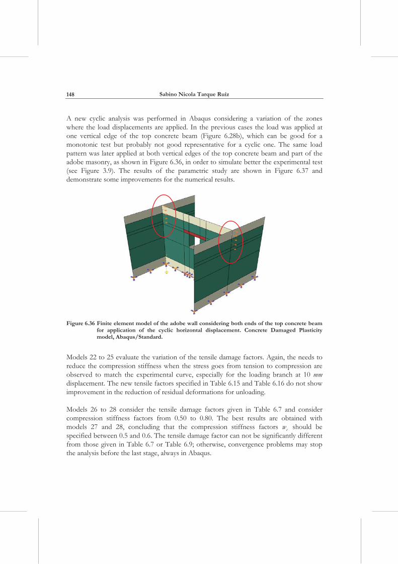
A new cyclic analysis was performed in Abaqus considering a variation of the zones where the load displacements are applied. In the previous cases the load was applied at one vertical edge of the top concrete beam (Figure 6.28b), which can be good for a monotonic test but probably not good representative for a cyclic one. The same load pattern was later applied at both vertical edges of the top concrete beam and part of the adobe masonry, as shown in Figure 6.36, in order to simulate better the experimental test (see Figure 3.9). The results of the parametric study are shown in Figure 6.37 and demonstrate some improvements for the numerical results.
Figure 6.36 Finite element model of the adobe wall considering both ends of the top concrete beam
for application of the cyclic horizontal displacement. Concrete Damaged Plasticity model, Abaqus/Standard.
Models 22 to 25 evaluate the variation of the tensile damage factors. Again, the needs to reduce the compression stiffness when the stress goes from tension to compression are observed to match the experimental curve, especially for the loading branch at 10 mm displacement. The new tensile factors specified in Table 6.15 and Table 6.16 do not show improvement in the reduction of residual deformations for unloading.
Models 26 to 28 consider the tensile damage factors given in Table 6.7 and consider compression stiffness factors from 0.50 to 0.80. The best results are obtained with models 27 and 28, concluding that the compression stiffness factors cw should be specified between 0.5 and 0.6. The tensile damage factor can not be significantly different from those given in Table 6.7 or Table 6.9; otherwise, convergence problems may stop the analysis before the last stage, always in Abaqus.
Numerical modelling of the seismic behaviour of adobe buildings
149
-50
-40
-30
-20
-10
0
10
20
30
40
50
-15 -10 -5 0 5 10 15
Displacement (mm)
Late
ral F
orce
(kN
)
ExperimentalNumerical model 22
-50
-40
-30
-20
-10
0
10
20
30
40
50
-15 -10 -5 0 5 10 15
Displacement (mm)
Late
ralF
orce
(kN
)
ExperimentalNumerical model 23
a) cw = 1, tw = 0, td = Table 6.7 b) cw = 1, tw = 0, td = Table 6.9
-50
-40
-30
-20
-10
0
10
20
30
40
50
-15 -10 -5 0 5 10 15
Displacement (mm)
Late
ral F
orce
(kN
)
ExperimentalNumerical model 24
-50
-40
-30
-20
-10
0
10
20
30
40
50
-15 -10 -5 0 5 10 15
Displacement (mm)
Late
ral F
orce
(kN
)
ExperimentalNumerical model 25
c) cw = 1, tw = 0, td = Table 6.15 d) cw = 1, tw = 0, td = Table 6.16
-50
-40
-30
-20
-10
0
10
20
30
40
50
-15 -10 -5 0 5 10 15
Displacement (mm)
Late
ral F
orce
(kN
)
ExperimentalNumerical model 26
-50
-40
-30
-20
-10
0
10
20
30
40
50
-15 -10 -5 0 5 10 15
Displacement (mm)
Late
ral F
orce
(kN
)
ExperimentalNumerical model 27
e) cw = 0.8, tw = 0, td = Table 6.7 f) cw = 0.6, tw = 0, td = Table 6.7
Figure 6.37. Comparison of the experimental and numerical cyclic behaviour of the adobe wall taking into account variability in the recovery stiffness and damage factors, in tension and compression. Horizontal load applied at both ends of the top concrete beam.
Sabino Nicola Tarque Ruíz
150
-50
-40
-30
-20
-10
0
10
20
30
40
50
-15 -10 -5 0 5 10 15
Displacement (mm)
Late
ral F
orce
(kN
)
ExperimentalNumerical model 28
g) cw = 0.5, tw = 0, td = Table 6.7
Figure 6.37. Continuation. Comparison of the experimental and numerical cyclic behaviour of the adobe wall taking into account variability in the recovery stiffness and damage factors. Horizontal load applied at both ends of the top concrete beam.
The Model 28 (Figure 6.37g) is used for showing the cracking process. From the analysis of the plastic strain it is seen that after the first 2 cycles of 1 mm some regions of the adobe masonry already exceed the maximum elastic strain. This effect is seen at the opening corners, where a concentration of tensile stresses is expected to occur (Figure 6.38a).
Figure 6.38 shows the formation process of tensile plastic strains at different values of the top displacement load in Model 28, where the most important aspect is the formation of the X-diagonal cracks, typical of the in-plane behaviour of masonry. The numerical results match the failure pattern seen in the experimental test (Figure 6.14). Horizontal cracks at the perpendicular walls are also formed due to bending.
a) Plastic strain values at the end of the 2 cycles of 1 mm
Figure 6.38. Formation process of the tensile plastic strain on the adobe wall under cyclic loads. A non unique legend in placed each to each figure to visualize better the plastic strain. Concrete damaged plasticity model, Abaqus/Standard.
Numerical modelling of the seismic behaviour of adobe buildings
151
c) Plastic strain values at the end of the cycle of 5 mm
d) Plastic strain values at the end of the cycle of 10 mm
Figure 6.38. Continuation. Formation process of the tensile plastic strain on the adobe wall under cyclic loads. A non unique legend in placed each to each figure to visualize better the plastic strain. Concrete damaged plasticity model, Abaqus/Standard.
Another way for interpretation of the tensile damage occurred in the adobe masonry is to show the tensile damage factor (Figure 6.39).
Figure 6.39. Tensile damage factor for Model 28 at the end of the history of cyclic horizontal
displacement load.
Sabino Nicola Tarque Ruíz
152
The tensile damage factor is a non-decreasing quantity associated with the tensile failure of the material. In Figure 6.39, the zones which are not in blue ( td = 0) indicate the zones which already are in the softening part of the tensile constitutive law and can be interpreted as damage zones.
6.6 VIBRATION MODES
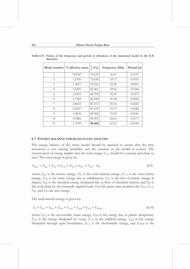
An eigenvalue analysis is done to compute the vibration modes of the model, especially in the direction of the applied load (X-X direction). The reinforced concrete beam placed as foundation of the wall is removed, so the total weight of the model is 100.63 kN. The base of the wall is fully fixed. The analysis is performed with Abaqus/Standard through the linear perturbation option and considering Lanczos method for extraction of the frequency values. A 50% of the elasticity of modulus has been used according to Tarque [2008] to take into account early cracking into the material. Figure 6.40 shows the effective mass related to the first 11 vibration modes, represented here by the frequency values. In theory the sum of all the effective masses should be equal to the total mass of the model. It is seen that 11 modes of vibration are required to reach the 90% of the total mass (Table 6.17), being the fundamental one the first mode.
0
10
20
30
40
50
60
70
80
8.644 18.753 25.583 29.053 36.399 41.283 45.337 53.734 55.388 58.641 61.147
Frequency (Hz)
Effe
ctiv
e m
ass
(%)
Figure 6.40. Contribution of the modes of vibration in the X-X direction until reaches the 90% of the
total mass of the model.
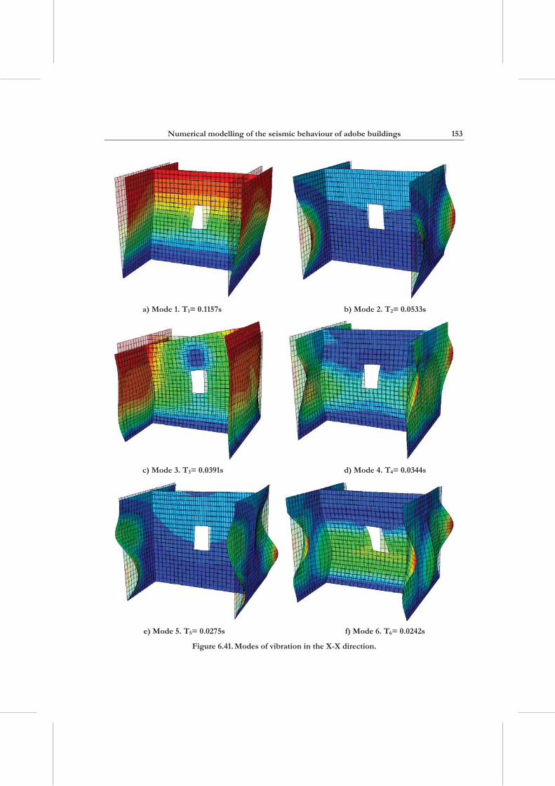
The deflected shapes given for each mode of vibration are shown in Figure 6.41. The first vibration mode, which involves 74.24% of the total mass, is a translational mode; while the others are basically out-of-plane deformations of the flange walls. This analysis considers the use of the elastic material properties. However, the adobe material is brittle and goes into the inelastic range very early; therefore the frequencies are expected to shorten.
Numerical modelling of the seismic behaviour of adobe buildings
153
a) Mode 1. T1= 0.1157s b) Mode 2. T2= 0.0533s
c) Mode 3. T3= 0.0391s d) Mode 4. T4= 0.0344s
e) Mode 5. T5= 0.0275s f) Mode 6. T6= 0.0242s
Figure 6.41. Modes of vibration in the X-X direction.
Sabino Nicola Tarque Ruíz
154
Table 6.17. Values of the frequency and period of vibrations of the numerical model in the X-X direction.
Mode number % effective mass (%) Frequency (Hz) Period (s)
1 74.2347 74.235 8.64 0.1157 2 1.1936 75.428 18.75 0.0533 3 1.5037 76.932 25.58 0.0391 4 5.5291 82.461 29.05 0.0344 5 2.2419 84.703 36.40 0.0275 6 1.7464 86.449 41.28 0.0242 7 0.8635 87.313 45.34 0.0221 8 0.2657 87.579 53.73 0.0186 9 1.4834 89.062 55.39 0.0181 10 0.0286 89.091 58.64 0.0171 11 1.3749 90.466 61.15 0.0164
6.7 ENERGY BALANCE FOR QUASI-STATIC ANALYSIS
The energy balance of the entire model should be checked to ensure that the time increment is not causing instability and the solution of the model is correct. The conservation of energy implies that the total energy Etotal should be constant and close to zero. The total energy is given by:
total KE IE VD SD KL JD WE E E E E E E E (6.9)
where EKE is the kinetic energy, EIE is the total internal energy, EVD is the visco-elastic energy, ESD is the static energy due to stabilization, EKL is the loss of kinetic energy at impact, EJD is the electrical energy dissipated due to flow of electrical current, and EW is the work done by the externally applied loads. For this quasi static problem the EKE, EVD, EKL and EJD are zero energy.
The total internal energy is given by:
I SE PD CD AE QB EE DMDE E E E E E E E (6.10)
where ESE is the recoverable strain energy, EPD is the energy due to plastic dissipation, ECD is the energy dissipated by creep, EAE is the artificial energy, EQB is the energy dissipated through quiet boundaries, EEE is the electrostatic energy, and EDMD is the
Numerical modelling of the seismic behaviour of adobe buildings
155
energy dissipated by damage. For the analysis made here the ECD, EQB, EEE are zero energy.
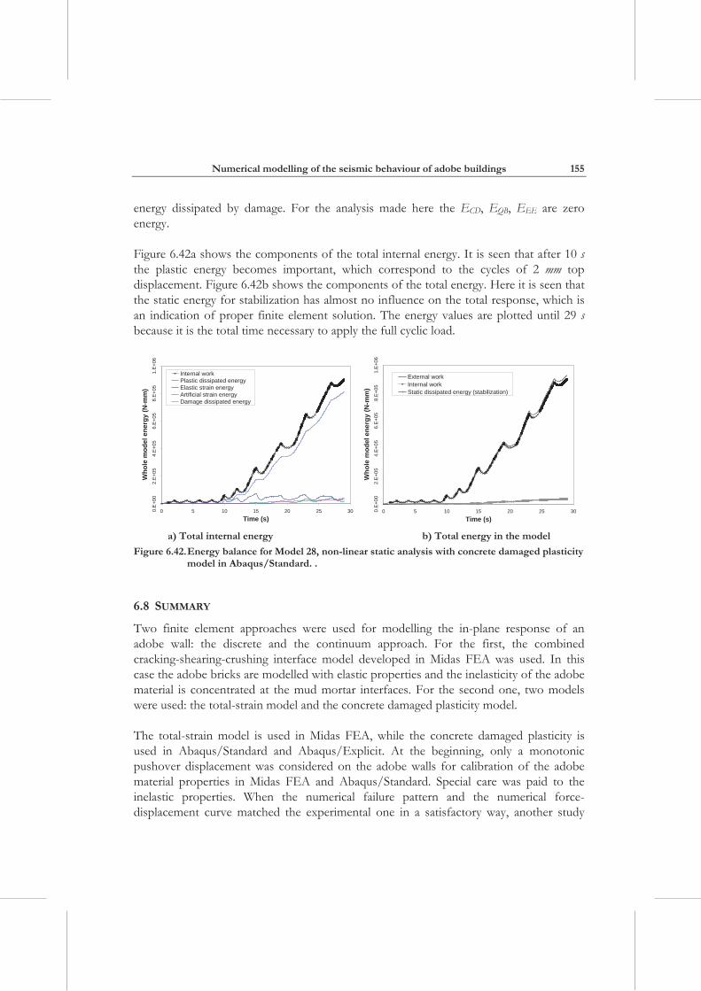
Figure 6.42a shows the components of the total internal energy. It is seen that after 10 s the plastic energy becomes important, which correspond to the cycles of 2 mm top displacement. Figure 6.42b shows the components of the total energy. Here it is seen that the static energy for stabilization has almost no influence on the total response, which is an indication of proper finite element solution. The energy values are plotted until 29 s because it is the total time necessary to apply the full cyclic load.
0.E
+00
2.E
+05
4.E
+05
6.E
+05
8.E
+05
1.E
+06
0 5 10 15 20 25 30Time (s)
Who
le m
odel
ene
rgy
(N-m
m)
Internal workPlastic dissipated energyElastic strain energyArtificial strain energyDamage dissipated energy
0.E+
002.
E+05
4.E+
056.
E+0
58.
E+0
51.
E+0
6
0 5 10 15 20 25 30Time (s)
Who
le m
odel
ene
rgy
(N-m
m)
External workInternal workStatic dissipated energy (stabilization)
a) Total internal energy b) Total energy in the model
Figure 6.42. Energy balance for Model 28, non-linear static analysis with concrete damaged plasticity model in Abaqus/Standard. .
6.8 SUMMARY
Two finite element approaches were used for modelling the in-plane response of an adobe wall: the discrete and the continuum approach. For the first, the combined cracking-shearing-crushing interface model developed in Midas FEA was used. In this case the adobe bricks are modelled with elastic properties and the inelasticity of the adobe material is concentrated at the mud mortar interfaces. For the second one, two models were used: the total-strain model and the concrete damaged plasticity model.
The total-strain model is used in Midas FEA, while the concrete damaged plasticity is used in Abaqus/Standard and Abaqus/Explicit. At the beginning, only a monotonic pushover displacement was considered on the adobe walls for calibration of the adobe material properties in Midas FEA and Abaqus/Standard. Special care was paid to the inelastic properties. When the numerical failure pattern and the numerical force-displacement curve matched the experimental one in a satisfactory way, another study
Sabino Nicola Tarque Ruíz
156
was done in Abaqus/Standard to simulate the cyclic response on an adobe wall. This way, damage factors and stiffness recovery in tension and compression were calibrated in view of the complete seismic analysis of adobe walls (see Chapter 7). The cyclic response was not able to be reproduced in Midas FEA due to difficulties in convergence for reversal loads.