6 large-scale-learning.pptx

Large-scale visual recognition Large-scale learning

Florent Perronnin, XRCE Hervé Jégou, INRIA

CVPR tutorial on Large-Scale Visual Recognition June 16, 2012

Motivation

Most popular image classification pipeline: BOV + SVMs ! See results of PASCAL VOC challenge http://pascallin.ecs.soton.ac.uk/challenges/VOC/

But can we scale SVMs to a dataset such as ImageNet…

… at a reasonable computational cost?

Outline

Efficient learning of linear classifiers with SGD

Non-linear classification with explicit embedding

An embedding view of the BOV and FV

Putting everything together

Learning with SGD Acknowledgement

The following slides are largely based on material available on Léon Bottou’s webpage: http://leon.bottou.org/projects/sgd

See also the excellent code available on the same webpage

Learning with SGD Historical note Stochastic Gradient Descent (SGD) was the standard for back-propagation training of Multi-Layer Perceptrons (MLP) LeCun, Bottou, Orr, Müller, “Efficient BackProp”, Neural Networks: Tricks of the trade”, Springer, 1998.

With the rise of large-margin classification algorithms (e.g. SVMs), MLPs fell somewhat into disuse… and so did SGD

Then, it was showed that SGD can be applied to large-margin classifiers with excellent properties Shalev-Swartz, Singer, Srebro, “Pegasos: Primal Estimated sub-GrAdient Solver for SVM”, ICML’07. Bottou, Bousquet, “The Tradeoffs of large scale learning”, NIPS’07. Shalev-Swartz, Srebro, “SVM optimization: inverse dependence on training set size”, ICML’08.

! Today very popular for large-scale learning

Learning with SGD Objective functions We consider objective functions of the form:

•! the zi’s correspond to the training samples •! w is the set of parameters to be learned

Linear two-class SVM example (primal formulation):

with

!

Learning with SGD Batch Gradient Descent (BGD) Iterative optimization algorithm:

where "t is the step size (e.g. line search)

!! assumes all samples are available in a large batch !! disk / memory requirements in O(N) !! slow convergence (more later)

Learning with SGD Stochastic Gradient Descent (SGD) Iterative optimization algorithm: •! pick a random sample zt

•! (noisy) update: where "t is the step size (e.g. fixed schedule)

"" disk/memory requirements in O(1) "" can handle new incoming samples "" faster convergence

Learning with SGD Convergence: BGD vs SGD Imagine you have 100 training samples and that you copy them 10 times ! 10x100 = 1,000 training samples

If we do one pass over the data: •! BGD: gradient with 100 samples = gradient with 1,000 samples ! computational cost x10 for the exact same result •! SGD: better results with the 1,000 samples than with 100 samples

! SGD exploits the redundancy in the training data

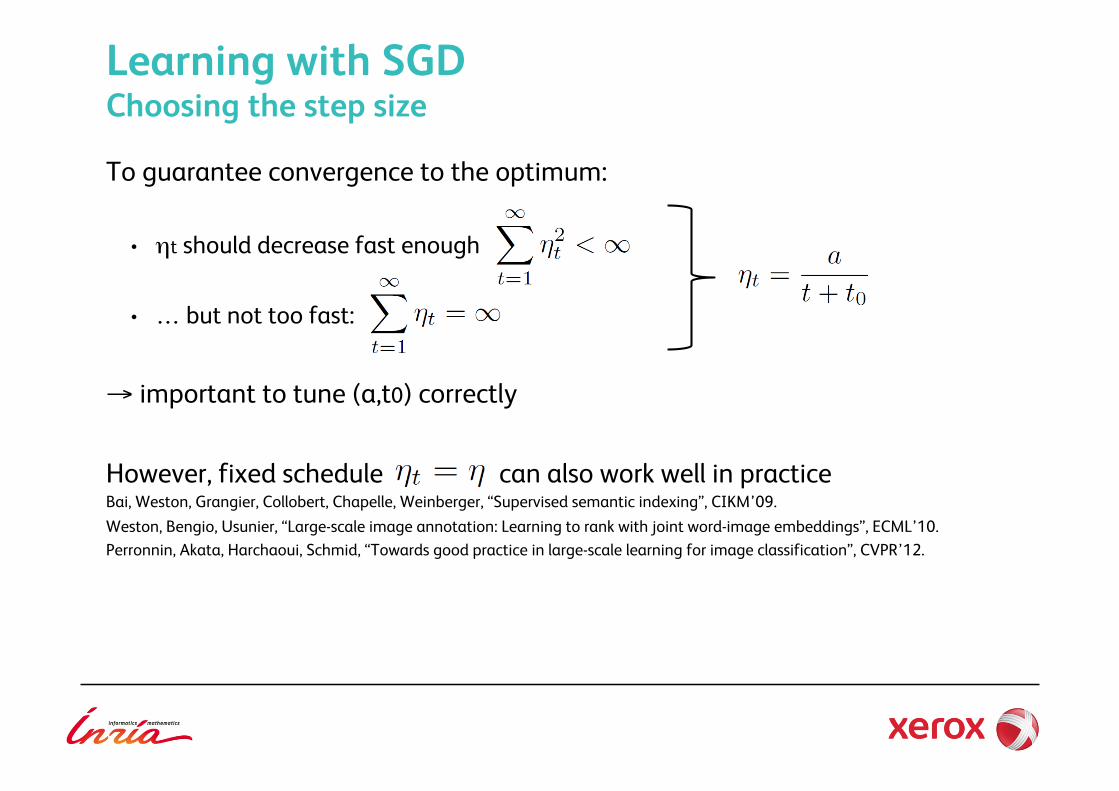
Learning with SGD Choosing the step size To guarantee convergence to the optimum:

•! "t should decrease fast enough …

•! … but not too fast:

! important to tune (a,t0) correctly

However, fixed schedule can also work well in practice Bai, Weston, Grangier, Collobert, Chapelle, Weinberger, “Supervised semantic indexing”, CIKM’09. Weston, Bengio, Usunier, “Large-scale image annotation: Learning to rank with joint word-image embeddings”, ECML’10. Perronnin, Akata, Harchaoui, Schmid, “Towards good practice in large-scale learning for image classification”, CVPR’12.

We have

with

Iteratively: •! pick a random sample zt=(xt,yt) •! update: with

! extremely simple to implement: few lines of code

Learning with SGD Linear two-class SVM example

Learning with SGD Beyond one-vs-rest

SGD is applicable to many optimization problems including: •! K-means clustering •! metric learning •! learning to rank •! multiclass learning •! structured learning •! etc.

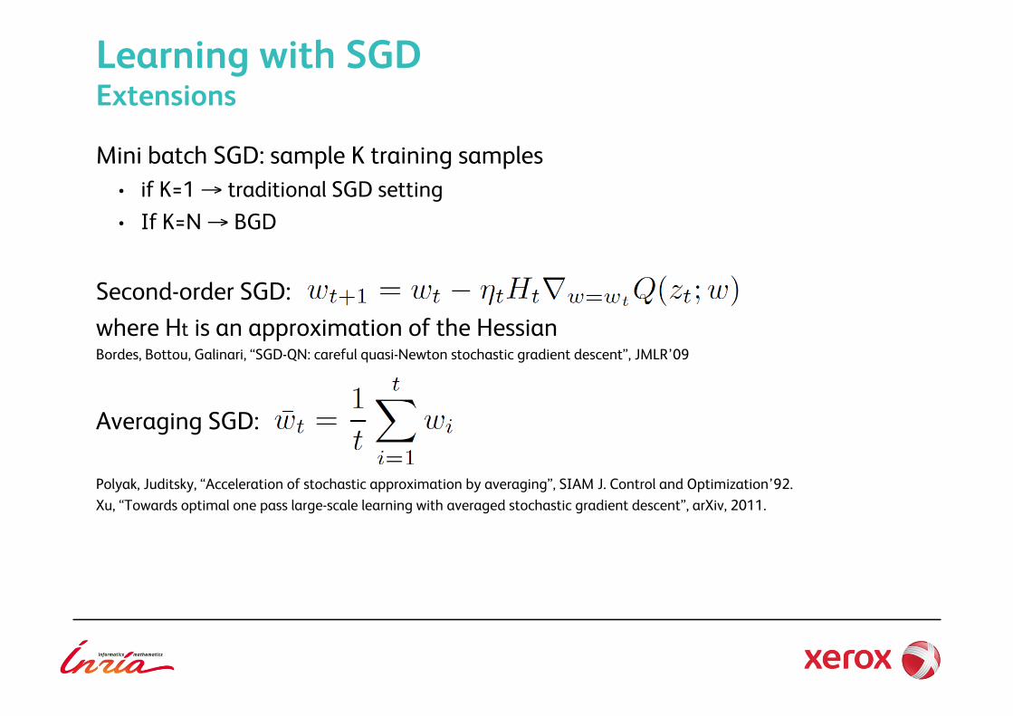
Learning with SGD Extensions Mini batch SGD: sample K training samples •! if K=1 ! traditional SGD setting •! If K=N ! BGD

Second-order SGD: where Ht is an approximation of the Hessian

Bordes, Bottou, Galinari, “SGD-QN: careful quasi-Newton stochastic gradient descent”, JMLR’09

Averaging SGD:

Polyak, Juditsky, “Acceleration of stochastic approximation by averaging”, SIAM J. Control and Optimization’92. Xu, “Towards optimal one pass large-scale learning with averaged stochastic gradient descent”, arXiv, 2011.

Learning with SGD Summary Very generic principle applicable to many algorithms

Very simple to implement… … but getting the step-size correct is not always trivial

Other online learning algorithms are closely related to SGD: e.g. Passive-Aggressive algorithms Crammer, Dekel, Keshet, Shaledv-Swartz, Singer, “Online passive-aggressive algorithms”, JMLR’06.

Best practices for large-scale learning of image classifiers : Perronnin, Akata, Harchaoui, Schmid, “Towards good practice in large-scale learning for image classification”, CVPR’12.

! a key conclusion: one-vs-rest is a competitive strategy with respect to more complex multiclass / ranking SVM formulations ! see also code available at http://lear.inrialpes.fr/src/jsgd/

Outline





Explicit embedding Kernels for the BOV Consider two families of non-linear kernels on BOV:

Additive Kernels: Exponential Kernels:

Explicit embedding Non-linear vs linear

We have just discussed how to train efficiently linear classifiers…

… Yet non-linear classifiers perform significantly better on the BOV: •! dense SIFT •! codebook with 4k visual words •! [1]: Léon Bottou’s SGD •! [2]: Chang and Lin’s LIBSVM

From: Perronnin, Sánchez and Liu, “Large-scale image categorization with explicit data embedding”, CVPR’10.

Can we get the accuracy of non-linear at the cost of linear?

PASCAL VOC 2007

Explicit embedding SVM formulations

Dual formulation: "" avoids explicit mapping of data in high-dimensional space !! training cost (e.g. SMO): between quadratic and cubic in # training samples !! runtime cost: linear in # support vectors

! Difficult to scale to very large image sets (e.g. ImageNet)

Primal formulation: !! requires explicit embedding of data in higher dimensional space "" training cost (e.g. SGD): linear in # training samples "" runtime cost: independent of # support vectors

!! Is explicit embedding such a high price to pay in large-scale?

Explicit embedding Primal formulation Positive definite kernel corresponds to implicit embedding:

The score becomes:

non-linear classification in the original space =

linear classification in the embedding space

Explicit embedding Principle

Non-linear classification with explicit embedding: •! perform an explicit (approximate) embedding of the data with •! learn linear classifiers in the new space (e.g. with efficient SGD)

Our focus: given a kernel, find

Generally a two-step procedure: •! find exact embedding function •! find good (i.e. accurate and efficient) approximation

Outline


Non-linear classification with explicit embedding: •! general case •! additive kernels •! exponential kernels



Problem: given an (unlabeled) training set with (M>E) find:

Kernel principal Component Analysis (kPCA): !! compute the MxM kernel matrix !! compute eigen-values / -vectors:

Embed a vector z with the Nyström approximation: !! project z:

!! embed:

Explicit embedding A generic solution: kPCA

Schölkopf, Smola and Müller, “Non-linear component analysis as a kernel eigenvalue problem”, Neural Computation’98. Williams and Seeger, “Using the Nystrom method to speed-up kernel machines”, NIPS’02.

Embedding cost: !! kernel matrix computation: O(M^2D) !! eigen-decomposition (incomplete Cholesky): O(M^2E) !! embedding one sample: O(M(D+E))

If we have N labeled training samples to learn our SVMs: !! kPCA embedding cost at training time: O(M(M+N)(D+E)) !! to be compared to direct kernel computation: O(N^2D)

"" works well if data lies in low-dimensional manifold (e.g. faces, digits) !! does not work so well on complex high-dimensional visual data

! Find specific solution for additive and exponential kernels

Explicit embedding A generic solution: kPCA

Outline




Kernels of the form:

Score becomes:

with

! Generalized Additive Model (GAM)

can be approximated by piecewise constant/linear functions. ! 1D functions enable efficient classification

Explicit embedding Additive kernels

Maji, Berg and Malik, “Classification using intersection kernel support vector machines is efficient”, CVPR’08.

Hastie and Tibshirani, “Generalized additive models”, Statistical Science’86.

Explicit embedding Additive kernels

Embedding 1D functions: find

such that

The final embedding function is given by:

Maji and Berg, “Max-margin additive classifiers for detection”, ICCV’09.

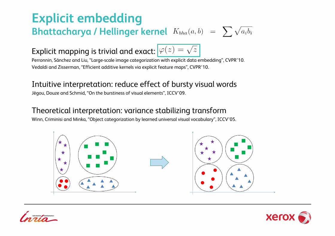
Explicit embedding Bhattacharya / Hellinger kernel Explicit mapping is trivial and exact: Perronnin, Sánchez and Liu, “Large-scale image categorization with explicit data embedding”, CVPR’10. Vedaldi and Zisserman, “Efficient additive kernels via explicit feature maps”, CVPR‘10.

Intuitive interpretation: reduce effect of bursty visual words Jégou, Douze and Schmid, “On the burstiness of visual elements”, ICCV’09.

Theoretical interpretation: variance stabilizing transform Winn, Criminisi and Minka, “Object categorization by learned universal visual vocabulary”, ICCV’05.

Introducing the indicator function:

we have:

How to approximate the ! dimensional feature map with a finite one? !! replace integral by sum

0 x z

1

Explicit embedding Intersection kernel

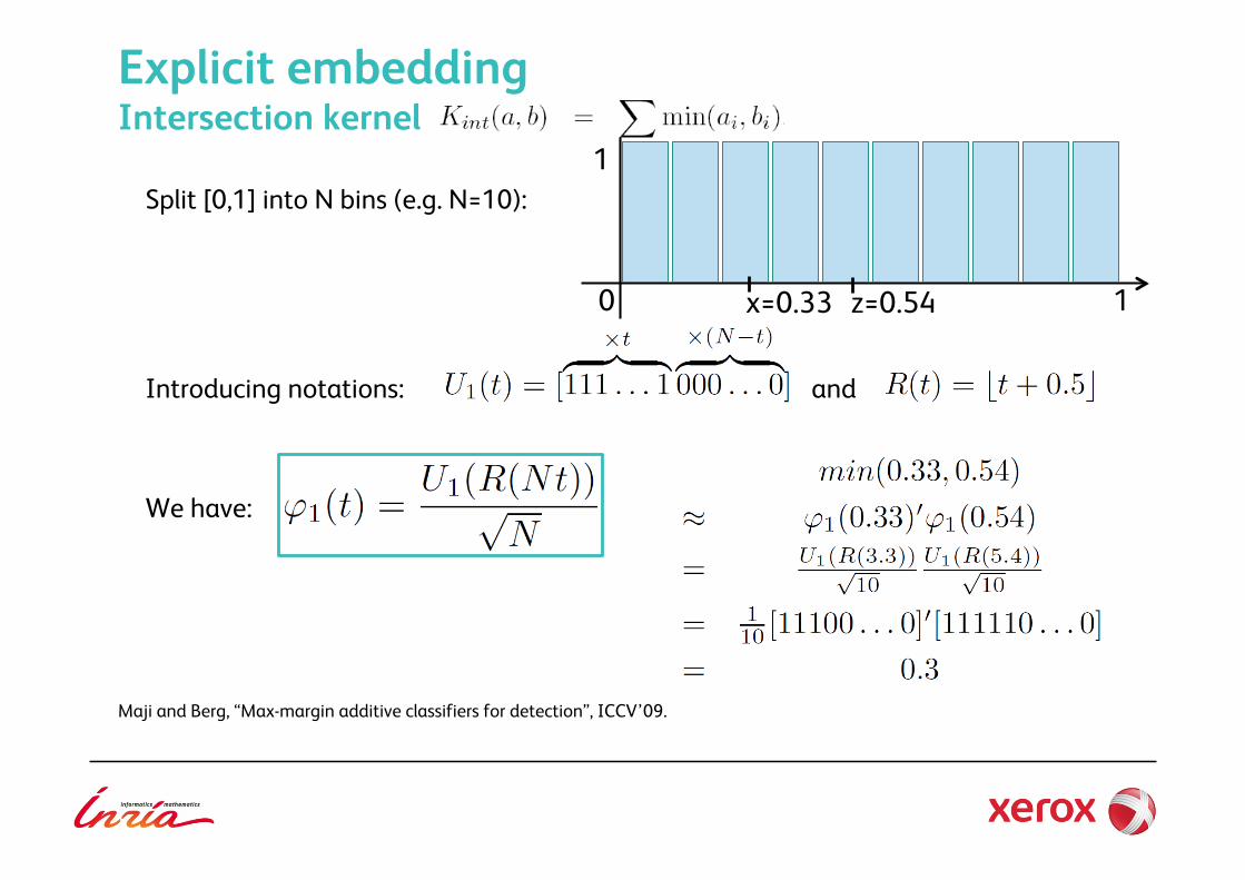
Split [0,1] into N bins (e.g. N=10):

Introducing notations: and

We have:


0 x=0.33 z=0.54

1

1


Split [0,1] into N bins (e.g. N=10):

Introducing notation:

We have:


0 x=0.33 z=0.54

1

1


"" As accurate as original kernel classifier "" Embedding is (almost) costless "" Embedded vectors can be sparsified: encode index (and residual) "" Training/classification uses simple look-up table accesses

!! Look-up table accesses can be much slower than standard arithmetic operations (e.g. addition, multiplication)

!! Embedding space is much larger than original space (e.g. x30) and linear classifiers are not sparse

See also: Wang, Hoiem and Forsyth, “Learning image similarity from Flickr groups using SIKMA”, ICCV’09.


Homogeneous kernels:

For any homogeneous kernel there exists a symmetric non-negative measure such that:

This can be rewritten as:

with ! closed form formulas exist for standard computer vision kernels

Hein and Bousquet, “Hilbertian metrics and positive definite kernels on probability measures”, AISTAT’05.

Vedaldi and Zisserman, “Efficient additive kernels via explicit feature maps”, CVPR’10.

Explicit embedding Additive homogeneous kernels

Explicit embedding Additive homogeneous kernels

How to approximate the ! dimensional feature map? ! sampling

and

with L the sampling step

Comparison with [Maji’09]:

"" Higher accuracy for same dimensionality

From: Vedaldi and Zisserman, “Efficient additive kernels via explicit feature maps”, CVPR’10.

Explicit embedding Additive kernels: general case

Going back to kernel kPCA: we can !! perform kPCA independently in each dimension !! concatenate dimension-wise embeddings

! Additive kPCA (addkPCA)

Embedding cost: !! computing D kernel matrices: O(M^2D) !! eigen-decomposition (Cholesky): O(M^2E) !! embedding of a sample: O(M(D+E))

! Same cost as kPCA? No as M much smaller for addkPCA!

"" Exploits data distribution: variable number of output embedding dimensions per input dimension Perronnin, Sánchez and Liu, “Large-scale image categorization with explicit data embedding”, CVPR’10.

Explicit embedding AddkPCA on Kchi2

Perronnin, Sánchez and Liu, “Large-scale image categorization with explicit data embedding”, CVPR’10.

Outline





Explicit embedding Shift-invariant kernels

Shift-invariant kernels:

Bochner’s theorem: a shift-invariant kernel is psd if and only if it is the Fourier transform of a non-negative measure p

Exact embedding:

with:

Approximate embedding by sampling: draw #’s iid from p

Rahimi and Recht, “Random features for large-scale kernel machines”, NIPS’07.

Explicit embedding Exponential kernels Example: RBF kernel ! p = Gaussian distribution But RBF kernel on BOV vectors does not perform well…

However, if we have: then we can write exponential kernels as shift-invariant:

Two-stage embedding process: •! embed additive kernel with any of the previous methods •! embed exponential kernel with random projections

Perronnin, Sánchez and Liu, “Large-scale image categorization with explicit data embedding”, CVPR’10. Vempati, Vedaldi, Zisserman and Jawahar, “Generalized RBF features maps for efficient detection”, BMVC’10.

Explicit embedding Results

E=D E=2D

E=3D

E=D

E=5D

E=10D

E=3D

E=2D E=D/4

E=D/2

E=D E=2D E=3D

Train on ImageNet, test on PASCAL VOC

Perronnin, Sánchez and Liu, “Large-scale image categorization with explicit data embedding”, CVPR’10.

Explicit embedding Summary

Explicit embedding works: from hours/days of training and testing to seconds/minutes!

In more detail: •! square-rooting the BOV already brings large improvements! •! additive kernels bring additional improvement at affordable cost •! exponential kernels bring additional gain at a significant cost

See also for a recent study: Gong and Lazebnik, “Comparing data-dependent and data-independent embeddings for classification and ranking of Internet images”, CVPR’11.

Is explicit embedding the only way to make linear classifiers work on BOV vectors? No!

Explicit embedding Max-pooling

The pooling strategy has a significant impact: max-pooling of local statistics superior to average pooling with linear classifiers.

Why? Reduces variance due to different proportions of foreground vs background information.

Example on Caltech 101: AVG POOLING MAX POOLING

LK IK LK IK

Hard Quantization 51.4 (0.9) 64.2 (1.0) 64.3 (0.9) 64.3 (0.9)

Soft Quantization 57.9 (1.5) 66.1 (1.2) 69.0 (0.8) 70.6 (1.0)

Sparse Coding 61.3 (1.3) 70.3 (1.3) 71.5 (1.1) 71.8 (1.0)

From [Boureau, CVPR’10]. LK = Linear kernel. IK = Intersection kernel.

Yang, Yu, Gong and Huang, “Linear spatial pyramid matching using sparse coding for image classification”, CVPR’09. Wang, Yang, Yu, Lv, Huang and Gong, “Locality-constrained Linear Coding for Image Classification”, CVPR’10

Boureau, Bach, LeCun and Ponce, “Learning mid-level features for recognition”, CVPR’10. See also: Boureau, Ponce and LeCun, “A Theoretical analysis of feature pooling in visual recognition”, ICML’10.

Outline





Embedding view of the BOV and FV

Embedding view of the BOV: !

So to obtain high-dim linearly separable BOV representations, we do : •! embed local descriptors individually •! average ! BOV histogram •! embed BOV histogram

! Aren’t two rounds of embeddings suboptimal?


Embedding view of the BOV: !

So to obtain high-dim linearly separable BOV representations, we do : •! embed local descriptors individually •! average ! BOV histogram •! embed BOV histogram

! Aren’t two rounds of embeddings suboptimal?

Fisher kernels can perform directly an embedding in much higher dim:

! works well in combination with linear classifiers

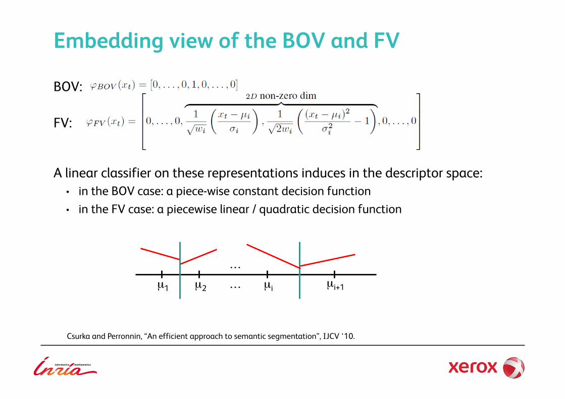
BOV:

FV:

A linear classifier on these representations induces in the descriptor space:


Csurka and Perronnin, “An efficient approach to semantic segmentation”, IJCV ‘10.

BOV:

FV:

A linear classifier on these representations induces in the descriptor space: •! in the BOV case: a piece-wise constant decision function



µ1 µ2 µi … µi+1

…

w1

w2

wi

wi+1

BOV:

FV:

A linear classifier on these representations induces in the descriptor space: •! in the BOV case: a piece-wise constant decision function •! in the FV case: a piecewise linear / quadratic decision function



µ1 µ2 µi … µi+1

…

BOV:

FV:

A linear classifier on these representations induces in the descriptor space: •! in the BOV case: a piece-wise constant decision function •! in the FV case: a piecewise linear / quadratic decision function

! FV leads to more complex decision functions for same vocabulary size



Outline




Putting everything together: •! large-scale pipelines •! large-scale results

BOV-based large-scale classification

BOV + explicit embedding + linear classifier

Memory / storage issue: embedding increases feature dim, e.g. x3 in [Vedaldi, CVPR’10] or [Perronnin, CVPR’10]

If embedding cost is low enough, efficient learning with SGD is possible: •! pick a random sample in original (low-dimensional) space •! embed sample on-the-fly in new (high-dimensional) space •! feed embedded sample to SGD routine •! discard embedded sample

FV-based large-scale classification

FV + linear classifier

Memory / storage issue: the FV is high-dim (e.g. "M dim) and weakly sparse ! Example using 4-byte floating point arithmetic: •! ILSVRC2010 # 2.8TBs •! ImageNet # 23TBs

… per low-level descriptor type

"" However, we can significantly compress FVs, e.g. using PQ Jégou, Douze and Schmid, “Product quantization for nearest neighbor search”, TPAMI’11. Jégou, Douze, Schmid and Pérez, “Aggregating local descriptors into a compact image representation”, CVPR’10.

! 64 fold compression with zero accuracy loss in categorization Sánchez and Perronnin, “High-dimensional signature compression for large-scale image classification”, CVPR’11.

FV-based large-scale classification

FV + PQ (at training time) + linear classifier

Efficient SGD learning algorithm: •! pick a random compressed sample •! decompress on-the-fly in high-dimensional space •! feed uncompressed sample to SGD routine •! discard uncompressed sample

! one decompressed sample alive in RAM at a time Sánchez and Perronnin, “High-dimensional signature compression for large-scale image classification”, CVPR’11.

Also possible to learn classifiers without decompression Vedaldi, Zisserman, “Sparse kernel approximations for efficient classification and detection”, CVPR’12.

Note: test samples do not need to be compressed

Outline




Putting everything together: •! large-scale pipelines •! large-scale results

Large-scale results Evaluation

How to measure accuracy when dealing with a large number of classes?

One cannot expect all images to be labeled with all possible classes ! Measure a top-K loss (e.g. K=5 in ILSVRC) Given a test image (labeled with G), predict labels L1, … LK

loss = mink d(G, Lk) with d(x,y) = 1 if x=y, 0 otherwise

Not all mistakes are equally bad ! Measure a hierarchical loss d(x,y) = height of lowest common ancestor of x and y / max. possible height

ImageNet Large-Scale Visual Recognition Challenge 2010: •! 1K classes (leaves only) •! 1.2M training images + 50K validation images + 150K test images •! measure top-5 accuracy (flat and hierarchical)

Berg, Deng and Fei-Fei, “Large-scale visual recognition challenge 2010”

Results on ILSVRC2010

Top 2 systems employed higher order statistics




No compression: training with Hadoop map-reduce (# 100 mappers) With PQ compression: training on a single server




FV + PQ compression + SGD learning

BOV + non-linear SVM in dual (GPU computing)

Results on ImageNet10K

Results on ImageNet10K: •! 10,184 classes (leaves and internal nodes) •! # 9M images: " training / " test •! accuracy measured as % top-1 correct



SIFT + BOV (21K-dim) + explicit embedding + linear SVM (SGD) !! accuracy = 6.4% !! training time # 6 CPU years Deng, Berg, Li and Fei-Fei, “What does classifying more than 10,000 image categories tell us?”, ECCV’10.



SIFT + BOV (21K-dim) + explicit embedding + linear SVM (SGD) !! accuracy = 6.4% !! training time # 6 CPU years Deng, Berg, Li and Fei-Fei, “What does classifying more than 10,000 image categories tell us?”, ECCV’10.

SIFT + FV (130K-dim) + PQ compression + linear SVM (SGD) !! accuracy = 19.1% !! training time # 1 CPU year (trick: do not sample all negatives) Perronnin, Akata, Harchaoui, Schmid, “Towards good practice in large-scale learning for image classification”, CVPR’12.

Questions?

6 large-scale-learning.pptx

Engineering

sgd convergence

sgd acknowledgement

largescale learning

training samples

sgd nonlinear classification

bgd vs sgd

sgd objective functions

learning florent perronnin