6 inverse kinematics - university of minnesota duluthrlindek1/me4135_11/ch6.pdf · 6. inverse...

6

Inverse KinematicsWhat are the joint variables for a given configuration of a robot? This isthe inverse kinematic problem. The determination of the joint variablesreduces to solving a set of nonlinear coupled algebraic equations. Althoughthere is no standard and generally applicable method to solve the inversekinematic problem, there are a few analytic and numerical methods tosolve the problem. The main difficulty of inverse kinematic is the multiplesolutions such as the one that is shown in Figure 6.1 for a planar 2Rmanipulator.

y2

y0

y1 x1

x0

x22θ

1θl 1

l2

FIGURE 6.1. Multiple solution for inverse kinematic problem of a planar 2Rmanipulator.

6.1 Decoupling Technique

Determination of joint variables in terms of the end-effector position andorientation is called inverse kinematics. Mathematically, inverse kinematicsis searching for the elements of vector q

q =£q1 q2 q3 · · · qn

¤T(6.1)

when a transformation 0Tn is given as a function of the joint variablesq1, q2, q3, · · · , qn .

0Tn =0T1(q1)

1T2(q2)2T3(q3)

3T4(q4) · · · n−1Tn(qn) (6.2)

R.N. Jazar, Theory of Applied Robotics, 2nd ed., DOI 10.1007/978-1-4419-1750-8_6, © Springer Science+Business Media, LLC 2010

326 6. Inverse Kinematics

Computer controlled robots are usually actuated in the joint variablespace, however objects to be manipulated are usually expressed in theglobal Cartesian coordinate frame. Therefore, carrying kinematic informa-tion, back and forth, between joint space and Cartesian space, is a need inrobotics. To control the configuration of the end-effector to reach an object,the inverse kinematics problem must be solved. Hence, we need to knowwhat the required values of joint variables are, to reach a desired point ina desired orientation.The result of forward kinematics of a 6 DOF robot is a 4 × 4 transfor-

mation matrix

0T6 = 0T11T2

2T33T4

4T55T6

=

⎡⎢⎢⎣r11 r12 r13 r14r21 r22 r23 r24r31 r32 r33 r340 0 0 1

⎤⎥⎥⎦ (6.3)

where 12 elements are trigonometric functions of six unknown joint vari-ables. However, because the upper left 3×3 submatrix of (6.3) is a rotationmatrix, only three elements of them are independent. This is because ofthe orthogonality condition (2.197). Hence, only six equations out of the12 equations of (6.3) are independent.Trigonometric functions inherently provide multiple solutions. Therefore,

multiple configurations of the robot are expected when the six equationsare solved for the unknown joint variables.It is possible to decouple the inverse kinematics problem into two sub-

problems, known as inverse position and inverse orientation kinematics.The practical consequence of such a decoupling is the allowance to breakthe problem into two independent problems, each with only three unknownparameters. Following the decoupling principle, the overall transformationmatrix of a robot can be decomposed to a translation and a rotation.

0T6 =

∙0R6

0d60 1

¸= 0D6

0R6 =

∙I 0d60 1

¸ ∙0R6 00 1

¸(6.4)

The translation matrix 0D6 indicates the position of the end-effector in B0and involves only the three joint variables of the manipulator. We can solve0d6 for the variables that control the wrist position. The rotation matrix0R6 indicates the orientation of the end-effector in B0 and involves onlythe three joint variables of the wrist. We can solve 0R6 for the variablesthat control the wrist orientation.

Proof. Most robots have a wrist made of three revolute joints with inter-secting and orthogonal axes at the wrist point. Taking advantage of having

6. Inverse Kinematics 327

a spherical wrist, we can decouple the kinematics of the wrist and manipu-lator by decomposing the overall forward kinematics transformation matrix0T6 into the wrist orientation and wrist position

0T6 =0T3

3T6 =

∙0R3

0d30 1

¸ ∙3R6 00 1

¸(6.5)

where the wrist orientation matrix is:

3R6 =0RT

30R6 =

0RT3

⎡⎣ r11 r12 r13r21 r22 r23r31 r32 r33

⎤⎦ (6.6)

and the wrist position vector is:

0d6 =

⎡⎣ r14r24r34

⎤⎦ (6.7)

The wrist position vector 0d6 ≡ 0d3 includes the manipulator joint vari-ables only. Hence, to solve the inverse kinematics of such a robot, we mustsolve 0d3 for position of the wrist point, and then solve 3R6 for orientationof the wrist.The components of the wrist position vector 0d6 = 0dwrist provides three

equations for the three unknown manipulator joint variables. Solving 0d6,for manipulator joint variables, leads to calculating 3R6 from (6.6). Then,the wrist orientation matrix 3R6 can be solved for wrist joint variables.In case we include the tool coordinate frame in forward kinematics, the

decomposition must be done according to the following equation to excludethe effect of tool distance d7 from the robot’s kinematics.

0T7 = 0T33T7 =

0T33T6

6T7

=

∙0R3 dw0 1

¸ ∙3R6 00 1

¸⎡⎢⎢⎣ I00d7

0 1

⎤⎥⎥⎦ (6.8)

In this case, inverse kinematics starts from determination of 0T6, which canbe found by

0T6 = 0T76T−17 (6.9)

= 0T7

⎡⎢⎢⎣1 0 0 00 1 0 00 0 1 d70 0 0 1

⎤⎥⎥⎦−1

= 0T7

⎡⎢⎢⎣1 0 0 00 1 0 00 0 1 −d70 0 0 1

⎤⎥⎥⎦ .


3θ

2θ

1θ

z2

z3z0x2

l3

l1

x0

y0

z1

x1l 2

P

x3

0dP

FIGURE 6.2. An R`RkR articulated manipulator.

Example 182 An articulated manipulator.Consider an articulated manipulator as is shown in Figure 6.2. The links

of the manipulator are R`R(90), RkR(0), R`R(90), and their associatedtransformation matrices between coordinate frames are:

0T1 =

⎡⎢⎢⎣cos θ1 0 sin θ1 0sin θ1 0 − cos θ1 00 1 0 l10 0 0 1

⎤⎥⎥⎦ (6.10)

1T2 =

⎡⎢⎢⎣cos θ2 − sin θ2 0 l2 cos θ2sin θ2 cos θ2 0 l2 sin θ20 0 1 00 0 0 1

⎤⎥⎥⎦ (6.11)

2T3 =

⎡⎢⎢⎣cos θ3 0 sin θ3 0sin θ3 0 − cos θ3 00 1 0 00 0 0 1

⎤⎥⎥⎦ (6.12)

The forward kinematics of the manipulator is:

0T3 = 0T11T2

2T3 (6.13)

=

⎡⎢⎢⎣cθ1c (θ2 + θ3) sθ1 cθ1s (θ2 + θ3) l2cθ1cθ2sθ1c (θ2 + θ3) −cθ1 sθ1s (θ2 + θ3) l2cθ2sθ1s (θ2 + θ3) 0 −c (θ2 + θ3) l1 + l2sθ2

0 0 0 1

⎤⎥⎥⎦


and therefore, the tip point P is at:

0dP =

⎡⎣ dxdydz

⎤⎦ = 0T3

⎡⎣ 00l3

⎤⎦=

⎡⎣ l3 sin (θ2 + θ3) cos θ1 + l2 cos θ1 cos θ2l3 sin (θ2 + θ3) sin θ1 + l2 sin θ1 cos θ2

l1 − l3 cos (θ2 + θ3) + l2 sin θ2

⎤⎦ (6.14)

Point P is supposed to be the point at which we attach a spherical wrist.Therefore, 0dP is the decoupled position vector of the wrist point that willnot be affected by the wrist attachment. 0dP provides three equations forthe three joint variables of the manipulator θ1, θ2, θ3. The first angle canbe found from

dx sin θ1 − dy cos θ1 = 0 (6.15)

that is:θ1 = atan2 (dy, dx) (6.16)

We combine the first and second elements of 0dP to find:

dx cos θ1 + dy sin θ1 = l3 sin (θ2 + θ3) + l2 cos θ2 (6.17)

Now, combining this equation and the third element of 0dP provides:

(dz − l1 − l2 sin θ2)2 + (dx cos θ1 + dy sin θ1 − l2 cos θ2)

2 = l23 (6.18)

or

−2l2 (dx cos θ1 + dy sin θ1) cos θ2 + 2l2 (l1 − dz) sin θ2 =

l23 −³(dx cos θ1 + dy sin θ1)

2+ l21 − 2l1dz + l22 + d2z

´(6.19)

that is a trigonometric equation of the form (6.88).

a cos θ2 + b sin θ2 = c (6.20)

a = −2l2 (dx cos θ1 + dy sin θ1)

b = 2l2 (l1 − dz)

c = l23 −³(dx cos θ1 + dy sin θ1)

2+ l21 − 2l1dz + l22 + d2z

´(6.21)

We solve this equation for θ2. Dividing (6.17) by the third element of 0dPdetermines θ3.

tan (θ2 + θ3) =dx cos θ1 + dy sin θ1 − l2 cos θ2

l1 + l2 sin θ2 − dz(6.22)

θ3 = atan2

µdx cos θ1 + dy sin θ1 − l2 cos θ2

l1 + l2 sin θ2 − dz

¶− θ2 (6.23)


Example 183 Numerical case of an articulated manipulator.To check the inverse kinematic equations of Example 182, let us examine

an articulated manipulator with the following dimensions

l1 = 1m

l2 = 1.05m

l3 = 0.89m (6.24)

when its tip point is at:

0dP =£1 1.1 1.2

¤T(6.25)

Equation (6.16) provides θ1.

θ1 = atan2 (dy, dx) = tan−1 1.1

1= 0.832 98 rad ≈ 47.727 deg (6.26)

To determine θ2, we should solve Equation (6.20)

a cos θ2 + b sin θ2 = c (6.27)

where,

a = −2l2 (dx cos θ1 + dy sin θ1) = −3.941263019 (6.28)

b = 2l2 (l1 − dz) = −0.5302360813 (6.29)

c = l23 −³(dx cos θ1 + dy sin θ1)

2+ l21 − 2l1dz + l22 + d2z

´= −3.232420149, − 5.232420149. (6.30)

We find two values for θ2 for c = −3.232

θ2 = 0.7555416816 rad ≈ 43.28934959 deg (6.31)

θ2 = −0.4880785028 rad ≈ −27.96483827 deg (6.32)

and we get no real answer for c = −5.232. θ3 comes from (6.23). If θ2 =0.755 rad then we have

θ3 = atan2

µdx cos θ1 + dy sin θ1 − l2 cos θ2

l1 + l2 sin θ2 − dz

¶− θ2

= .1913201914 rad ≈ 11 deg (6.33)

and if θ2 = −0.488 rad then we have:

θ3 = −.1913201910 rad ≈ −11 deg (6.34)


Example 184 Inverse kinematics for a 2R planar manipulator.Figure 5.9 illustrates a 2R planar manipulator with two RkR links ac-

cording to the coordinate frames setup shown in the figure. The forwardkinematics of the manipulator was found to be

0T2 = 0T11T2 (6.35)

=

⎡⎢⎢⎣c (θ1 + θ2) −s (θ1 + θ2) 0 l1cθ1 + l2c (θ1 + θ2)s (θ1 + θ2) c (θ1 + θ2) 0 l1sθ1 + l2s (θ1 + θ2)

0 0 1 00 0 0 1

⎤⎥⎥⎦ .The inverse kinematics of planar robots are generally easier to find analyt-ically. The global position of the tip point of the manipulator is at∙

XY

¸=

∙l1 cos θ1 + l2 cos (θ1 + θ2)l1 sin θ1 + l2 sin (θ1 + θ2)

¸(6.36)

thereforeX2 + Y 2 = l21 + l22 + 2l1l2 cos θ2 (6.37)

and

cos θ2 =X2 + Y 2 − l21 − l22

2l1l2(6.38)

θ2 = cos−1X2 + Y 2 − l21 − l22

2l1l2. (6.39)

However, we usually avoid using arcsin and arccos because of the inaccu-racy. So, we employ the half angle formula

tan2θ

2=1− cos θ1 + cos θ

(6.40)

to find θ2 using an atan2 function

θ2 = ±2 atan2

s(l1 + l2)

2 − (X2 + Y 2)

(X2 + Y 2)− (l1 − l2)2 . (6.41)

The ± is because of the square root, which generates two solutions. Thesetwo solutions are called elbow up and elbow down, as shown in Figure6.3(a) and (b) respectively.The first joint variable θ1 of an elbow up configuration can geometrically

be found from

θ1 = atan2Y

X+ atan2

l2 sin θ2l1 + l2 cos θ2

(6.42)

and for an elbow down configuration from

θ1 = atan2Y

X− atan2 l2 sin θ2

l1 + l2 cos θ2. (6.43)


y2

Y

y1x1

X

l2

x2

x2y2

Y

y1

l1

l 2

x1

(a) (b)

l 1

2θ

1θ2θ

1θX

FIGURE 6.3. Illustration of a 2R planar manipulator in two possible configura-tions: (a) elbow up and (b) elbow down.

θ1 can also be found from the following alternative equation.

θ1 = atan2−Xl2 sin θ2 + Y (l1 + l2 cos θ2)

Y l2 sin θ2 +X (l1 + l2 cos θ2)(6.44)

Most of the time, the value of θ1 should be corrected by adding or subtractingπ depending on the sign of X. It is also possible to combine Equations of(6.36) and determine a trigonometric equation for θ1.

2Xl1 cos θ1 + 2Y l1 sin θ1 = X2 + Y 2 + l21 − l22 (6.45)

It is also convenient to use the following equation.

l1 + l2 cos θ2 =X2 + Y 2 + l21 − l22

2l1(6.46)

The two different sets of solutions for θ1 and θ2 correspond to the elbow upand elbow down configurations.

Example 185 Motion of a 2R manipulator.Consider a 2R planar manipulator with

l1 = 1m l1 = 1m (6.47)

that its tip point is moving from P1 (1.2, 1.5) to P2 (−1.2, 1.5) on a straightline. The using the inverse kinematic equations (6.39) and (6.42), we candetermine the configuration of the manipulator at any point of the path.Figure 6.4 illustrates the manipulator at 42 equally spaced points betweenP1 and P2. Let us assume that the tip point is moving of the line based on


X

Y

P2 P1

FIGURE 6.4. A 2R planar manipulator with l1 = 1m, l1 = 1m moving from P1to P2 on a straight line.

the following time behavior.

X = 1.2− t Y = 1.5 0 ≤ t ≤ 2.4 (6.48)

The variation of the angles θ1 and θ2 are as shown in Figure 6.5.

Example 186 Inverse kinematics of an articulated robot.The forward kinematics of the articulated robot, illustrated in Figure 6.6,

was found in Example 166, where the overall transformation matrix of theend-effector was found, based on the wrist and arm transformation matri-ces.

0T7 = TarmTwrist =0T3

3T7

The wrist transformation matrix Twrist is described in (5.124) and the ma-nipulator transformation matrix, Tarm is found in (5.74). However, accord-ing to a new setup coordinate frame, as shown in Figure 6.6, we have a 6Rrobot with a six links configuration

1 R`R(90)2 RkR(0)3 R`R(90)4 R`R(−90)5 R`R(90)6 RkR(0)

and a displacement TZ,d7 . Therefore, the individual links’ transformation


t

1θ

2θ

deg

FIGURE 6.5. The variation of the angles θ1 and θ2 of the 2R planar manipulatorof Figure 6.4.

z0

Base

Shoulder

ElbowForearm

z1

z5

z4

z6

x3

z3

x5x6

x4

z7

y7d7

Gripper

l2

Wrist point

y2

x0

z2

d2l3

y1

1θ

2θ3θ

4θ

5θ 6θ

x8x9

FIGURE 6.6. A 6 DOF articulated manipulator.


matrices are

0T1 =


⎤⎥⎥⎦ (6.49)

1T2 =

⎡⎢⎢⎣cos θ2 − sin θ2 0 l2 cos θ2sin θ2 cos θ2 0 l2 sin θ20 0 1 d20 0 0 1

⎤⎥⎥⎦ (6.50)

2T3 =


⎤⎥⎥⎦ (6.51)

3T4 =

⎡⎢⎢⎣cos θ4 0 − sin θ4 0sin θ4 0 cos θ4 00 −1 0 l30 0 0 1

⎤⎥⎥⎦ (6.52)

4T5 =


⎤⎥⎥⎦ (6.53)

5T6 =

⎡⎢⎢⎣cos θ6 − sin θ6 0 0sin θ6 cos θ6 0 00 0 1 00 0 0 1

⎤⎥⎥⎦ (6.54)

6T7 =

⎡⎢⎢⎣1 0 0 00 1 0 00 0 1 d60 0 0 1

⎤⎥⎥⎦ (6.55)

and the tool transformation matrix in the base coordinate frame is

0T7 = 0T11T2

2T33T4

4T55T6

6T7 (6.56)

= 0T33T6

6T7

=

⎡⎢⎢⎣t11 t12 t13 t14t21 t22 t23 t24t31 t32 t33 t340 0 0 1

⎤⎥⎥⎦


where

0T3 =

⎡⎢⎢⎣cθ1c(θ2 + θ3) sθ1 cθ1s(θ2 + θ3) l2cθ1cθ2 + d2sθ1sθ1c(θ2 + θ3) −cθ1 sθ1s(θ2 + θ3) l2cθ2sθ1 − d2cθ1s(θ2 + θ3) 0 −c(θ2 + θ3) l2sθ2

0 0 0 1

⎤⎥⎥⎦(6.57)

3T6 =

⎡⎢⎢⎣cθ4cθ5cθ6 − sθ4sθ6 −cθ6sθ4 − cθ4cθ5sθ6 cθ4sθ5 0cθ5cθ6sθ4 + cθ4sθ6 cθ4ccθ6 − cθ5sθ4sθ6 sθ4sθ5 0

−cθ6sθ5 sθ5sθ6 cθ5 l30 0 0 1

⎤⎥⎥⎦(6.58)

and

t11 = cθ1 (c (θ2 + θ3) (cθ4cθ5cθ6 − sθ4sθ6)− cθ6sθ5s (θ2 + θ3))

+sθ1 (cθ4sθ6 + cθ5cθ6sθ4) (6.59)

t21 = sθ1 (c (θ2 + θ3) (−sθ4sθ6 + cθ4cθ5cθ6)− cθ6sθ5s (θ2 + θ3))

−cθ1 (cθ4sθ6 + cθ5cθ6sθ4) (6.60)

t31 = s (θ2 + θ3) (cθ4cθ5cθ6 − sθ4sθ6) + cθ6sθ5c (θ2 + θ3) (6.61)

t12 = cθ1 (sθ5sθ6s (θ2 + θ3)− c (θ2 + θ3) (cθ6sθ4 + cθ4cθ5sθ6))

+sθ1 (cθ4cθ6 − cθ5sθ4sθ6) (6.62)

t22 = sθ1 (sθ5sθ6s (θ2 + θ3)− c (θ2 + θ3) (cθ6sθ4 + cθ4cθ5sθ6))

+cθ1 (−cθ4cθ6 + cθ5sθ4sθ6) (6.63)

t32 = −sθ5sθ6c (θ2 + θ3)− s (θ2 + θ3) (cθ6sθ4 + cθ4cθ5sθ6) (6.64)

t13 = sθ1sθ4sθ5 + cθ1 (cθ5s (θ2 + θ3) + cθ4sθ5c (θ2 + θ3)) (6.65)

t23 = −cθ1sθ4sθ5 + sθ1 (cθ5s (θ2 + θ3) + cθ4sθ5c (θ2 + θ3)) (6.66)

t33 = cθ4sθ5s (θ2 + θ3)− cθ5c (θ2 + θ3) (6.67)

t14 = d6 (sθ1sθ4sθ5 + cθ1 (cθ4sθ5c (θ2 + θ3) + cθ5s (θ2 + θ3)))

+l3cθ1s (θ2 + θ3) + d2sθ1 + l2cθ1cθ2 (6.68)

t24 = d6 (−cθ1sθ4sθ5 + sθ1 (cθ4sθ5c (θ2 + θ3) + cθ5s (θ2 + θ3)))

+sθ1s (θ2 + θ3) l3 − d2cθ1 + l2cθ2sθ1 (6.69)

t34 = d6 (cθ4sθ5s (θ2 + θ3)− cθ5c (θ2 + θ3))

+l2sθ2 + l3c (θ2 + θ3) . (6.70)

Solution of the inverse kinematics problem starts with the wrist positionvector d, which is

£t14 t24 t34

¤Tof 0T7 for d7 = 0

d =

⎡⎣ cθ1 (l3s (θ2 + θ3) + l2cθ2) + d2sθ1sθ1 (l3s (θ2 + θ3) + l2cθ2)− d2cθ1

l3c (θ2 + θ3) + l2sθ2

⎤⎦ =⎡⎣ dx

dydz

⎤⎦ . (6.71)


Theoretically, we must be able to solve Equation (6.71) for the three jointvariables θ1, θ2, and θ3. It can be seen that

dx sin θ1 − dy cos θ1 = d2 (6.72)

which provides

θ1 = 2atan2(dx ±qd2x + d2y − d22, d2 − dy). (6.73)

Equation (6.73) has two solutions for d2x + d2y > d22, one solution ford2x + d2y = d22 , and no real solution for d

2x + d2y < d22.

Combining the first two elements of d gives

l3 sin (θ2 + θ3) = ±qd2x + d2y − d22 − l2 cos θ2 (6.74)

then, the third element of d may be utilized to find

l23 =³±qd2x + d2y − d22 − l2 cos θ2

´2+ (dz − l2 sin θ2)

2 (6.75)

which can be rearranged to the following form

a cos θ2 + b sin θ2 = c (6.76)

a = 2l2

qd2x + d2y − d22 (6.77)

b = 2l2dz (6.78)

c = d2x + d2y + d2z − d22 + l22 − l23. (6.79)

with two solutions

θ2 = atan2(c

r,±r1− c2

r2)− atan2(a, b) (6.80)

r2 = a2 + b2. (6.81)

Summing the squares of the elements of d gives

d2x + d2y + d2z = d22 + l22 + l23 + 2l2l3 sin (2θ2 + θ3) (6.82)

that provides

θ3 = arcsin

Ãd2x + d2y + d2z − d22 − l22 − l23

2l2l3

!− 2θ2. (6.83)

Having θ1, θ2, and θ3 means we can find the wrist point in space. How-ever, because the joint variables in 0T3 and in 3T6 are independent, we


should find the orientation of the end-effector by solving 3T6 or 3R6 for θ4,θ5, and θ6.

3R6 =

⎡⎣ cθ4cθ5cθ6 − sθ4sθ6 −cθ6sθ4 − cθ4cθ5sθ6 cθ4sθ5cθ5cθ6sθ4 + cθ4sθ6 cθ4ccθ6 − cθ5sθ4sθ6 sθ4sθ5

−cθ6sθ5 sθ5sθ6 cθ5

⎤⎦=

⎡⎣ s11 s12 s13s21 s22 s23s31 s32 s33

⎤⎦ (6.84)

The angles θ4, θ5, and θ6 can be found by examining elements of 3R6

θ4 = atan2 (s23, s13) (6.85)

θ5 = atan2

µqs213 + s223, s33

¶(6.86)

θ6 = atan2 (s32,−s31) . (6.87)

Example 187 F Solution of trigonometric equation a cos θ+ b sin θ = c.The first type of trigonometric equation

a cos θ + b sin θ = c (6.88)

can be solved by introducing two new variables r and φ such that

a = r sinφ (6.89)

b = r cosφ (6.90)

and

r =pa2 + b2 (6.91)

φ = atan2(a, b). (6.92)

Substituting the new variables show that

sin(φ+ θ) =c

r(6.93)

cos(φ+ θ) = ±r1− c2

r2. (6.94)

Hence, the solutions of the problem are

θ = atan2(c

r,±r1− c2

r2)− atan2(a, b) (6.95)

orθ = atan2(c,±

pr2 − c2)− atan2(a, b). (6.96)


Therefore, the equation a cos θ + b sin θ = c has two solutions if r2 = a2 +b2 > c2, one solution if r2 = c2, and no solution if r2 < c2.As an example, let us solve the following equation.

1.5 cos θ + 2.5 sin θ = 2.549 (6.97)

Having a = 1.5 and b = 2.5, we find r and φ.

r =pa2 + b2 = 2.915475947 (6.98)

φ = atan2(a, b) = 0.5404195 rad (6.99)

Therefore,

θ = atan2(c,±pr2 − c2)− atan2(a, b)

= atan2(2.549,±√2)− φ

= 0.5235718477 rad, 1.537181805 rad

≈ 30 deg, 88.07 deg (6.100)

Example 188 F Meaning of the function tan−12yx = atan2(y, x).

In robotic calculation, specially in solving inverse kinematic problems,we need to find an angle based on the sin and cos functions of the angle.However, tan−1 cannot show the effect of the individual sign for the numer-ator and denominator. It always represents an angle in the first or fourthquadrant. To overcome this problem and determine the joint angles in thecorrect quadrant, the atan2 function is introduced as:

atan2(y, x) =

⎧⎪⎪⎪⎪⎪⎨⎪⎪⎪⎪⎪⎩sgn y tan−1

¯yx

¯if x > 0, y 6= 0

π

2sgn y if x = 0, y 6= 0

sgn y³π − tan−1

¯yx

¯´if x < 0, y 6= 0

π − π sgnx if x 6= 0, y = 0

(6.101)

The sgn represents the signum function.

sgn(x) =

⎧⎨⎩ 1 if x > 00 if x = 0−1 if x < 0

(6.102)

As an example, let us compare the tan−1 and atan2 for four points in fourquadrants.

x = 1, y = 1 then tan−1 11 = 0.785 atan2(1, 1) = 0.785x = −1, y = 1 then tan−1 1

−1 = −0.785 atan2(1,−1) = 2.356x = −1, y = −1 then tan−1 −1−1 = 0.785 atan2(−1,−1) = −2.356x = 1, y = −1 then tan−1 −11 = −0.785 atan2(−1, 1) = −0.785

In this text, whether it has been mentioned or not, wherever tan−1 yx is

used, it must be calculated based on atan2(y, x).


Example 189 F Fundamental properties of arcsin and arccos.The general solution of equations

sinϕ = a cos θ = b tanψ = c (6.103)

are:

ϕ = sin−1 a = (−1)k sin−1 a+ kπ (6.104)

θ = cos−1 b = ± cos−1 b+ 2kπ (6.105)

ψ = tan−1 c = tan−1 c+ kπ c2 6= −1 (6.106)

Example 190 F General inverse kinematics formulas.There are some general trigonometric equations that regularly appear in

inverse kinematics problems. The following indicates the most frequentlyequations and solutions.

1. Ifsin θ = a (6.107)

then, we have two answers: θ and π − θ.

θ = atan2a

±√1− a2

(6.108)

2. Ifcos θ = b (6.109)

then, we have two answers: θ and −θ.

θ = atan2±√1− b2

b(6.110)

3. Ifsin θ = a cos θ = b (6.111)

then,θ = atan2

a

b. (6.112)

4. Ifa cos θ + b sin θ = 0 (6.113)

then, we have two answers: θ and θ + π.

θ = atan2a

bθ = atan2

−a−b (6.114)

5. Ifa cos θ + b sin θ = c (6.115)

then,

θ = atan2a

b+ atan2

±√a2 + b2 − c2

c. (6.116)


6. If

a cos θ + b sin θ = c (6.117)

a cos θ − b sin θ = d (6.118)

then,

a2 + b2 = c2 + d2 (6.119)

θ = atan2ac− bd

ad+ bc. (6.120)

7. Ifsin θ sinϕ = a cos θ sinϕ = b (6.121)

then, we have two answers: θ and θ + π.

θ = atan2a

bθ = atan2

−a−b (6.122)

8. Ifsin θ sinϕ = a cos θ sinϕ = b cosϕ = c (6.123)

then, we have two answers for θ and ϕ: θ corresponds to ϕ, and θ+πcorresponds to −ϕ.

θ = atan2a

bθ = atan2

−a−b (6.124)

ϕ = atan2

√a2 + b2

cϕ = atan2

−√a2 + b2

c(6.125)

6.2 Inverse Transformation Technique

Assume we have the transformation matrix 0T6 indicating the global posi-tion and the orientation of the end-effector of a 6 DOF robot in the baseframe B0. Furthermore, assume the geometry and individual transforma-tion matrices 0T1(q1), 1T2(q2), 2T3(q3), 3T4(q4), 4T5(q5), and 5T6(q6) aregiven as functions of joint variables.According to forward kinematics,

0T6 = 0T11T2

2T33T4

4T55T6 (6.126)

=

⎡⎢⎢⎣r11 r12 r13 r14r21 r22 r23 r24r31 r32 r33 r340 0 0 1

⎤⎥⎥⎦ .


We can solve the inverse kinematics problem by solving the following equa-tions for the unknown joint variables:

1T6 = 0T−110T6 (6.127)

2T6 = 1T−120T−11

0T6 (6.128)3T6 = 2T−13

1T−120T−11

0T6 (6.129)4T6 = 3T−14

2T−131T−12

0T−110T6 (6.130)

5T6 = 4T−153T−14

2T−131T−12

0T−110T6 (6.131)

I = 5T−164T−15

3T−142T−13

1T−120T−11

0T6 (6.132)

Proof. We multiply both sides of the transformation matrix 0T6 by 0T−11to obtain

0T−110T6 = 0T−11

¡0T1

1T22T3

3T44T5

5T6¢

= 1T6. (6.133)

Note that 0T−11 is the mathematical inverse of the 4×4 matrix 0T1, and notan inverse transformation. So, 0T−11 must be calculated by a mathematicalmatrix inversion.The left-hand side of Equation (6.133) is a function of q1. However, the

elements of the matrix 1T6 on the right-hand side are either zero, constant,or functions of q2, q3, q4, q5, and q6. The zero or constant elements of theright-hand side provides the required algebraic equation to be solved forq1.Then, we multiply both sides of (6.133) by 1T−12 to obtain

1T−120T−11

0T6 = 1T−120T−11

¡0T1

1T22T3

3T44T5

5T6¢

= 2T6. (6.134)

The left-hand side of this equation is a function of q2, while the elements ofthe matrix 2T6, on the right hand side, are either zero, constant, or functionsof q3, q4, q5, and q6. Equating the associated element, with constant or zeroelements on the right-hand side, provides the required algebraic equationto be solved for q2.Following this procedure, we can find the joint variables q3, q4, q5, and

q6 by using the following equalities respectively.

2T−131T−12

0T−110T6

= 2T−131T−12

0T−11¡0T1

1T22T3

3T44T5

5T6¢

= 3T6.(6.135)

3T−142T−13

1T−120T−11

0T6= 3T−14

2T−131T−12

0T−11¡0T1

1T22T3

3T44T5

5T6¢

= 4T6.(6.136)


3θ

2θ

1θ

z2

z3z0 x2

l3

l1

x0

y0

z1

x1l 2

P

x3

0dP

x4

z4

FIGURE 6.7. An articulated manipulator.

4T−153T−14

2T−131T−12

0T−110T6

= 4T−153T−14

2T−131T−12

0T−11¡0T1

1T22T3

3T44T5

5T6¢

= 5T6.(6.137)

5T−164T−15

3T−142T−13

1T−120T−11

0T6= 5T−16

4T−153T−14

2T−131T−12

0T−11¡0T1

1T22T3

3T44T5

5T6¢

= I.(6.138)

The inverse transformation technique may sometimes be called Piepertechnique.

Example 191 Articulated manipulator and numerical case.Consider the articulated manipulator shown in Figure 6.7. The transfor-

mation matrices between its coordinate frames are:

0T1 =

⎡⎢⎢⎣cos θ1 0 sin θ1 0sin θ1 0 − cos θ1 00 1 0 l10 0 0 1

⎤⎥⎥⎦ (6.139)

1T2 =


⎤⎥⎥⎦ (6.140)


2T3 =


⎤⎥⎥⎦ (6.141)

The forward kinematics of the manipulator is:

0T3 = 0T11T2

2T3 (6.142)

=

⎡⎢⎢⎣cθ1c (θ2 + θ3) sθ1 cθ1s (θ2 + θ3) l2cθ1cθ2sθ1c (θ2 + θ3) −cθ1 sθ1s (θ2 + θ3) l2cθ2sθ1s (θ2 + θ3) 0 −c (θ2 + θ3) l1 + l2sθ2

0 0 0 1

⎤⎥⎥⎦Point P is supposed to be the point at which we attach a spherical wrist.Therefore, we attach a takht coordinate frame B4 at P that is at a constantdistance l3 from B3.

3T4 =

⎡⎢⎢⎣1 0 0 00 1 0 00 0 1 l30 0 0 1

⎤⎥⎥⎦ (6.143)

So, the overall forward kinematics of the manipulator is:

0T4 =0T3

3T4 = (6.144)⎡⎢⎢⎣cθ1c (θ2 + θ3) sθ1 cθ1s (θ2 + θ3) l3s (θ2 + θ3) cθ1 + l2cθ1cθ2sθ1c (θ2 + θ3) −cθ1 sθ1s (θ2 + θ3) l3s (θ2 + θ3) sθ1 + l2cθ2sθ1s (θ2 + θ3) 0 −c (θ2 + θ3) l1 − l3c (θ2 + θ3) + l2sθ2

0 0 0 1

⎤⎥⎥⎦Using the following dimensions

l1 = 1m l2 = 1.05m l3 = 0.89m (6.145)

when its tip point is at:

0dP =£1 1.1 1.2

¤T(6.146)

the forward kinematics reduces to:

0T4 =

⎡⎢⎢⎣cos (θ2 + θ3) cos θ1 sin θ1 sin (θ2 + θ3) cos θ1 1cos (θ2 + θ3) sin θ1 − cos θ1 sin (θ2 + θ3) sin θ1 1.1sin (θ2 + θ3) 0 − cos (θ2 + θ3) 1.2

0 0 0 1

⎤⎥⎥⎦(6.147)

Let us multiply both sides by 0T−11 to have:

0T−110T4 =

0T−11¡0T1

1T22T3

3T4¢= 1T4 (6.148)


where,

0T−110T4 = 1T4 =

⎡⎢⎢⎣cos θ1 sin θ1 0 00 0 1 −1

sin θ1 − cos θ1 0 00 0 0 1

⎤⎥⎥⎦ 0T4 (6.149)

=

⎡⎢⎢⎣cos (θ2 + θ3) 0 sin (θ2 + θ3) cos θ1 + 1.1 sin θ1sin (θ2 + θ3) 0 − cos (θ2 + θ3) 0.2

0 1 0 sin θ1 − 1.1 cos θ10 0 0 1

⎤⎥⎥⎦and

1T22T3

3T4 = (6.150)⎡⎢⎢⎣c (θ2 + θ3) 0 s (θ2 + θ3) 1.2s (θ2 + θ3) + 1.1cθ2s (θ2 + θ3) 0 −c (θ2 + θ3) 1.1sθ2 − 1.2c (θ2 + θ3)

0 1 0 00 0 0 1

⎤⎥⎥⎦ .The last column of the left hand side of (6.148) is only a function of θ1while the right hand side is a function of θ2 and θ3. Equating the elementr24 of both sides of (6.148) provides an equation to determine θ1.

sin θ1 − 1.1 cos θ1 = 0 (6.151)

θ1 = atan2 (1.1, 1) = tan−11.1

1= 0.8329812667 rad ≈ 47.72631098 deg (6.152)

Substituting θ1 = 0.832 98 rad in (6.149) provides a matrix 1T4 with a nu-merical values in the last column.

1T4 =

⎡⎢⎢⎣cos (θ2 + θ3) 0 sin (θ2 + θ3) 1.486 6sin (θ2 + θ3) 0 − cos (θ2 + θ3) 0.2

0 1 0 00 0 0 1

⎤⎥⎥⎦ (6.153)

We multiply both sides of (6.153) by 1T−12 to have:1T−12

1T4 =1T−12

¡1T2

2T33T4¢= 2T4 (6.154)

where,

1T−121T4 = 2T4 =

⎡⎢⎢⎣cos θ2 sin θ2 0 −1.05− sin θ2 cos θ2 0 00 0 1 00 0 0 1

⎤⎥⎥⎦ 1T4 (6.155)

=

⎡⎢⎢⎣cos θ3 0 sin θ3 1.486 6 cos θ2 + 0.2 sin θ2 − 1.05sin θ3 0 − cos θ3 0.2 cos θ2 − 1.486 6 sin θ20 1 0 00 0 0 1

⎤⎥⎥⎦


and

2T33T4 =

⎡⎢⎢⎣cos θ3 0 sin θ3 0.89 sin θ3sin θ3 0 − cos θ3 −0.89 cos θ30 1 0 00 0 0 1

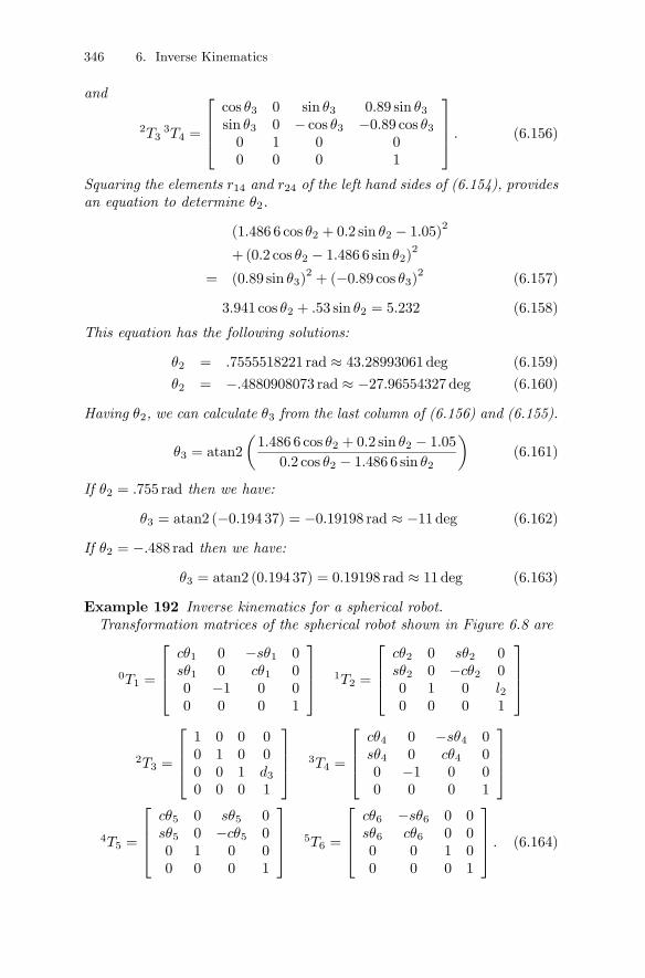
⎤⎥⎥⎦ . (6.156)

Squaring the elements r14 and r24 of the left hand sides of (6.154), providesan equation to determine θ2.

(1.486 6 cos θ2 + 0.2 sin θ2 − 1.05)2

+(0.2 cos θ2 − 1.486 6 sin θ2)2

= (0.89 sin θ3)2+ (−0.89 cos θ3)2 (6.157)

3.941 cos θ2 + .53 sin θ2 = 5.232 (6.158)

This equation has the following solutions:

θ2 = .7555518221 rad ≈ 43.28993061 deg (6.159)

θ2 = −.4880908073 rad ≈ −27.96554327 deg (6.160)

Having θ2, we can calculate θ3 from the last column of (6.156) and (6.155).

θ3 = atan2

µ1.486 6 cos θ2 + 0.2 sin θ2 − 1.050.2 cos θ2 − 1.486 6 sin θ2

¶(6.161)

If θ2 = .755 rad then we have:

θ3 = atan2 (−0.194 37) = −0.19198 rad ≈ −11 deg (6.162)

If θ2 = −.488 rad then we have:

θ3 = atan2 (0.194 37) = 0.19198 rad ≈ 11 deg (6.163)

Example 192 Inverse kinematics for a spherical robot.Transformation matrices of the spherical robot shown in Figure 6.8 are

0T1 =

⎡⎢⎢⎣cθ1 0 −sθ1 0sθ1 0 cθ1 00 −1 0 00 0 0 1

⎤⎥⎥⎦ 1T2 =

⎡⎢⎢⎣cθ2 0 sθ2 0sθ2 0 −cθ2 00 1 0 l20 0 0 1

⎤⎥⎥⎦

2T3 =

⎡⎢⎢⎣1 0 0 00 1 0 00 0 1 d30 0 0 1

⎤⎥⎥⎦ 3T4 =

⎡⎢⎢⎣cθ4 0 −sθ4 0sθ4 0 cθ4 00 −1 0 00 0 0 1

⎤⎥⎥⎦4T5 =

⎡⎢⎢⎣cθ5 0 sθ5 0sθ5 0 −cθ5 00 1 0 00 0 0 1

⎤⎥⎥⎦ 5T6 =

⎡⎢⎢⎣cθ6 −sθ6 0 0sθ6 cθ6 0 00 0 1 00 0 0 1

⎤⎥⎥⎦ . (6.164)


l2

z2

d3

z1

z0

d7

z3

z4

z5z7

x2

x1

x0

x3x4

x5x7z6x6

Link 1

Link 2

Link 3

2θ

1θ

5θ

4θ 6θ

FIGURE 6.8. A spherical robot, made of a spherical manipulator attached to aspherical wrist.

Therefore, the position and orientation of the end-effector for a set of jointvariables, which solves the forward kinematics problem, can be found bymatrix multiplication

0T6 = 0T11T2

2T33T4

4T55T6

=

⎡⎢⎢⎣r11 r12 r13 r14r21 r22 r23 r24r31 r32 r33 r340 0 0 1

⎤⎥⎥⎦ (6.165)

where the elements of 0T6 are the same as the elements of the matrix inEquation (5.159).Multiplying both sides of the (6.165) by 0T−11 provides

0T−110T6 =

⎡⎢⎢⎣cos θ1 sin θ1 0 00 0 −1 0

− sin θ1 cos θ1 0 00 0 0 1

⎤⎥⎥⎦⎡⎢⎢⎣

r11 r12 r13 r14r21 r22 r23 r24r31 r32 r33 r340 0 0 1

⎤⎥⎥⎦

=

⎡⎢⎢⎣f11 f12 f13 f14f21 f22 f23 f24f31 f32 f33 f340 0 0 1

⎤⎥⎥⎦ (6.166)


where

f1i = r1i cos θ1 + r2i sin θ1 (6.167)

f2i = −r3i (6.168)

f3i = r2i cos θ1 − r1i sin θ1 (6.169)

i = 1, 2, 3, 4.

Based on the given transformation matrices, we find that

1T6 = 1T22T3

3T44T5

5T6

=

⎡⎢⎢⎣f11 f12 f13 f14f21 f22 f23 f24f31 f32 f33 f340 0 0 1

⎤⎥⎥⎦ (6.170)

f11 = −cθ2sθ4sθ6 + cθ6 (−sθ2sθ5 + cθ2cθ4cθ5) (6.171)

f21 = −sθ2sθ4sθ6 + cθ6 (cθ2sθ5 + cθ4cθ5sθ2) (6.172)

f31 = cθ4sθ6 + cθ5cθ6sθ4 (6.173)

f12 = −cθ2cθ6sθ4 − sθ6 (−sθ2sθ5 + cθ2cθ4cθ5) (6.174)

f22 = −cθ6sθ2sθ4 − sθ6 (cθ2sθ5 + cθ4cθ5sθ2) (6.175)

f32 = cθ4cθ6 − cθ5sθ4sθ6 (6.176)

f13 = cθ5sθ2 + cθ2cθ4sθ5 (6.177)

f23 = −cθ2cθ5 + cθ4sθ2sθ5 (6.178)

f33 = sθ4sθ5 (6.179)

f14 = d3sθ2 (6.180)

f24 = −d3cθ2 (6.181)

f34 = l2. (6.182)

The only constant element of the matrix (6.170) is f34 = l2, therefore,

r24 cos θ1 − r14 sin θ1 = l2. (6.183)

This kind of trigonometric equation frequently appears in robotic inversekinematics, which has a systematic method of solution. We assume

r14 = r cosφ (6.184)

r24 = r sinφ (6.185)


l2

d3

z1

z0

z3

x3

x0x2

z21θ

FIGURE 6.9. Left shoulder configuration of a spherical robot.

wherer =

qr214 + r224 (6.186)

φ = tan−1r24r14

(6.187)

and therefore, Equation (6.183) becomes

l2r= sinφ cos θ1 − cosφ sin θ1 = sin(φ− θ1) (6.188)

showing that±p1− (l2/r)2 = cos(φ− θ1). (6.189)

Hence, the solution of Equation (6.183) for θ1 is

θ1 = tan−1 r24

r14− tan−1 l2

±pr2 − l22

. (6.190)

The (−) sign corresponds to a left shoulder configuration of the robotsas shown in Figure 6.9, and the (+) sign corresponds to the right shoulderconfiguration.The elements f14 and f24 of matrix (6.170) are functions of θ1 and θ2

only.

f14 = d3 sin θ2 = r14 cos θ1 + r24 sin θ1 (6.191)

f24 = −d3 cos θ2 = −r34 (6.192)


Hence, it is possible to use them and find θ2

θ2 = tan−1 r14 cos θ1 + r24 sin θ1

r34(6.193)

where θ1 must be substituted from (6.190).In the next step, we find the third joint variable d3 from

1T−120T−11

0T6 =2T6 (6.194)

where

1T−12 =

⎡⎢⎢⎣cos θ2 sin θ2 0 00 0 1 −l2

sin θ2 − cos θ2 0 00 0 0 1

⎤⎥⎥⎦ (6.195)

and

2T6 =

⎡⎢⎢⎣−sθ4sθ6 + cθ4cθ5cθ6 −cθ6sθ4 − cθ4cθ5sθ6 cθ4sθ5 0cθ4sθ6 + cθ5cθ6sθ4 cθ4cθ6 − cθ5sθ4sθ6 sθ4sθ5 0

−cθ6sθ5 sθ5sθ6 cθ5 d30 0 0 1

⎤⎥⎥⎦ .(6.196)

Employing the elements of the matrices on both sides of Equation (6.194)shows that the element (3, 4) can be utilized to find d3.

d3 = r34 cos θ2 + r14 cos θ1 sin θ2 + r24 sin θ1 sin θ2 (6.197)

Since there is no other element in Equation (6.194) to be a function ofanother single variable, we move to the next step and evaluate θ4 from

3T−142T−13

1T−120T−11

0T6 =4T6 (6.198)

because 2T−131T−12

0T−110T6 =

3T6 provides no new equation. Evaluating4T6

4T6 =

⎡⎢⎢⎣cos θ5 cos θ6 − cos θ5 sin θ6 sin θ5 0cos θ6 sin θ5 − sin θ5 sin θ6 − cos θ5 0sin θ6 cos θ6 0 00 0 0 1

⎤⎥⎥⎦ (6.199)

and the left-hand side of (6.198) utilizing

2T−13 =

⎡⎢⎢⎣1 0 0 00 1 0 00 0 1 −d30 0 0 1

⎤⎥⎥⎦ (6.200)


and

3T−14 =

⎡⎢⎢⎣cos θ4 sin θ4 0 00 0 −1 0

− sin θ4 cos θ4 0 00 0 0 1

⎤⎥⎥⎦ (6.201)

shows that

3T−142T−13

1T−120T−11

0T6 =

⎡⎢⎢⎣g11 g12 g13 g14g21 g22 g23 g24g31 g32 g33 g340 0 0 1

⎤⎥⎥⎦ (6.202)

where

g1i = −r3icθ4sθ2 + r2i (cθ1sθ4 + cθ2cθ4sθ1)

+r1i (−sθ1sθ4 + cθ1cθ2cθ4) (6.203)

g2i = d3δ4i − r31cθ2 − r11cθ1sθ2 − r21sθ1sθ2 (6.204)

g3i = r31sθ2sθ4 + r21 (cθ1cθ4 − cθ2sθ1sθ4)

+r11 (−cθ4sθ1 − cθ1cθ2sθ4) (6.205)

i = 1, 2, 3, 4.

The symbol δ4i indicates the Kronecker delta and is:

δ4i =

½1 if i = 40 if i 6= 4 (6.206)

Therefore, we can find θ4 by equating the element (3, 3), θ5 by equatingthe elements (1, 3) or (2, 3), and θ6 by equating the elements (3, 1) or (3, 2).Starting from element (3, 3)

r13 (−cθ4sθ1 − cθ1cθ2sθ4) + r23 (cθ1cθ4 − cθ2sθ1sθ4) + r33sθ2sθ4 = 0(6.207)

we find θ4

θ4 = tan−1 −r13sθ1 + r23cθ1

cθ2 (r13cθ1 + r23sθ1)− r33sθ2(6.208)

which, based on the second value of θ1, can also be equal to

θ4 =π

2+ tan−1

−r13sθ1 + r23cθ1cθ2 (r13cθ1 + r23sθ1)− r33sθ2

. (6.209)

Now we use elements (1, 3) and (2, 3),

sin θ5 = r23 (cos θ1 sin θ4 + cos θ2 cos θ4 sin θ1)− r33 cos θ4 sin θ2

+r13 (cos θ1 cos θ2 cos θ4 − sin θ1 sin θ4) (6.210)

− cos θ5 = −r33 cos θ2 − r13 cos θ1 sin θ2 − r23 sin θ1 sin θ2 (6.211)


to find θ5

θ5 = tan−1 sin θ5cos θ5

. (6.212)

Finally, θ6 can be found from the elements (3, 1) and (3, 2)

sin θ6 = r31 sin θ2 sin θ4 + r21 (cos θ1 cos θ4 − cos θ2 sin θ1 sin θ4)+r11 (− cos θ4 sin θ1 − cos θ1 cos θ2 sin θ4) (6.213)

cos θ6 = r32 sin θ2 sin θ4 + r22 (cos θ1 cos θ4 − cos θ2 sin θ1 sin θ4)+r12 (− cos θ4 sin θ1 − cos θ1 cos θ2 sin θ4) (6.214)

θ6 = tan−1 sin θ6cos θ6

. (6.215)

Example 193 Inverse of parametric Euler angles transformation matrix.The global rotation matrix based on Euler angles has been found in Equa-

tion (2.107).

GRB = [Az,ψ Ax,θ Az,ϕ]T = RZ,ϕRX,θ RZ,ψ

=

⎡⎣ cϕcψ − cθsϕsψ −cϕsψ − cθcψsϕ sθsϕcψsϕ+ cθcϕsψ −sϕsψ + cθcϕcψ −cϕsθ

sθsψ sθcψ cθ

⎤⎦=

⎡⎣ r11 r12 r13r21 r22 r23r31 r32 r33

⎤⎦ (6.216)

Premultiplying GRB by R−1Z,ϕ, gives⎡⎣ cosϕ sinϕ 0

− sinϕ cosϕ 00 0 1

⎤⎦ GRB

=

⎡⎣ r11cϕ+ r21sϕ r12cϕ+ r22sϕ r13cϕ+ r23sϕr21cϕ− r11sϕ r22cϕ− r12sϕ r23cϕ− r13sϕ

r31 r32 r33

⎤⎦=

⎡⎣ cosψ − sinψ 0cos θ sinψ cos θ cosψ − sin θsin θ sinψ sin θ cosψ cos θ

⎤⎦ . (6.217)

Equating the elements (1, 3) of both sides

r13 cosϕ+ r23 sinϕ = 0 (6.218)

givesϕ = atan2 (r13,−r23) . (6.219)


Having ϕ helps us to find ψ by using elements (1, 1) and (1, 2)

cosψ = r11 cosϕ+ r21 sinϕ (6.220)

− sinψ = r12 cosϕ+ r22 sinϕ (6.221)

therefore,

ψ = atan2−r12 cosϕ− r22 sinϕ

r11 cosϕ+ r21 sinϕ. (6.222)

In the next step, we may postmultiply GRB by R−1Z,ψ, to provide

GRB

⎡⎣ cosψ sinψ 0− sinψ cosψ 00 0 1

⎤⎦=

⎡⎣ r11cψ − r12sψ r12cψ + r11sψ r13r21cψ − r22sψ r22cψ + r21sψ r23r31cψ − r32sψ r32cψ + r31sψ r33

⎤⎦=

⎡⎣ cosϕ − cos θ sinϕ sin θ sinϕsinϕ cos θ cosϕ − cosϕ sin θ0 sin θ cos θ

⎤⎦ . (6.223)

The elements (3, 1) on both sides make an equation to find ψ.

r31 cosψ − r31 sinψ = 0 (6.224)

Therefore, it is possible to find ψ from the following equation:

ψ = atan2 (r31, r31) . (6.225)

Finally, θ can be found using elements (3, 2) and (3, 3)

r32cψ + r31sψ = sin θ (6.226)

r33 = cos θ (6.227)

which give

θ = atan2r32 cosψ + r31 sinψ

r33. (6.228)

Example 194 Inverse of given Euler angles transformation matrix.Assume the global rotation matrix based on Euler angles is given as:

GRB = [Az,ψ Ax,θ Az,ϕ]T = RZ,ϕRX,θ RZ,ψ

=

⎡⎣ cϕcψ − cθsϕsψ −cϕsψ − cθcψsϕ sθsϕcψsϕ+ cθcϕsψ −sϕsψ + cθcϕcψ −cϕsθ

sθsψ sθcψ cθ

⎤⎦=

⎡⎣ 0.126 83 −0.780 33 0.612 370.926 78 −0.126 83 −0.353 550.353 55 0.612 37 0.707 11

⎤⎦ (6.229)


Premultiplying GRB by R−1Z,ϕ, gives⎡⎣ cosϕ sinϕ 0

− sinϕ cosϕ 00 0 1

⎤⎦ GRB

=

⎡⎣ 0.126cϕ+ 0.926sϕ −0.780cϕ− 0.126sϕ 0.612cϕ− 0.353sϕ0.926cϕ− 0.126sϕ 0.780sϕ− 0.126cϕ −0.353cϕ− 0.612sϕ

0.353 55 0.612 37 0.707 11

⎤⎦=

⎡⎣ cosψ − sinψ 0cos θ sinψ cos θ cosψ − sin θsin θ sinψ sin θ cosψ cos θ

⎤⎦ . (6.230)

Equating the elements (1, 3) of both sides

0.612 37 cosϕ− 0.353 55 sinϕ = 0 (6.231)

gives

ϕ = atan2

µ0.612 37

0.353 55

¶= 1.0472 rad = 60 deg . (6.232)

Having ϕ helps us to find ψ by using elements (1, 1) and (1, 2)

cosψ = 0.126 cosϕ+ 0.926 sinϕ (6.233)

− sinψ = −0.78 cosϕ− 0.126 sinϕ (6.234)

therefore,

ψ = atan20.78 cosϕ+ 0.126 sinϕ

0.126 cosϕ+ 0.926 sinϕ

= atan20.499 12

0.864 94= 0.523 rad = 30deg . (6.235)

Although we can find θ from elements (2, 3) and (3, 3), let us postmultiplyGRB by R

−1Z,ψ, to follow the inverse transformation technique.

GRB

⎡⎣ cosψ sinψ 0− sinψ cosψ 00 0 1

⎤⎦=

⎡⎣ 0.126cψ + 0.78sψ 0.126sψ − 0.78cψ 0.612 370.926cψ + 0.126sψ 0.926sψ − 0.126cψ −0.353 550.353cψ − 0.612sψ 0.612cψ + 0.353sψ 0.707 11

⎤⎦=

⎡⎣ cosϕ − cos θ sinϕ sin θ sinϕsinϕ cos θ cosϕ − cosϕ sin θ0 sin θ cos θ

⎤⎦ (6.236)

The elements (3, 1) on both sides make an equation to find ψ.

0.353 55 cosψ − 0.612 37 sinψ = 0 (6.237)


Therefore, it is also possible to find ψ from the following equation:

ψ = atan2

µ0.353 55

0.612 37

¶= 0.523 rad = 30 deg (6.238)

Finally, θ can be found using elements (3, 2) and (3, 3)

0.612 37 cosψ + 0.353 55 sinψ = sin θ (6.239)

0.707 11 = cos θ (6.240)

which give

θ = atan20.707 11

0.707 11= 1 rad = 45 deg . (6.241)

Example 195 F Inverse kinematics and nonstandard DH frames.Consider a 3 DOF planar manipulator shown in Figure 5.4. The non-

standard DH transformation matrices of the manipulator are

0T1 =


⎤⎥⎥⎦ (6.242)

1T2 =

⎡⎢⎢⎣cos θ2 − sin θ2 0 l1sin θ2 cos θ2 0 00 0 1 00 0 0 1

⎤⎥⎥⎦ (6.243)

2T3 =

⎡⎢⎢⎣cos θ3 − sin θ3 0 l2sin θ3 cos θ3 0 00 0 1 00 0 0 1

⎤⎥⎥⎦ (6.244)

3T4 =

⎡⎢⎢⎣1 0 0 l30 1 0 00 0 1 00 0 0 1

⎤⎥⎥⎦ . (6.245)

The solution of the inverse kinematics problem is a mathematical problemand none of the standard or nonstandard DH methods for defining linkframes provide any simplicity. To calculate the inverse kinematics, we start


with calculating the forward kinematics transformation matrix 0T4

0T4 = 0T11T2

2T33T4 (6.246)

=

⎡⎢⎢⎣cos θ123 − sin θ123 0 l1 cos θ1 + l2 cos θ12 + l3 cos θ123sin θ123 cos θ123 0 l1 sin θ1 + l2 sin θ12 + l3 sin θ1230 0 1 00 0 0 1

⎤⎥⎥⎦

=

⎡⎢⎢⎣r11 r12 r13 r14r21 r22 r23 r24r31 r32 r33 r340 0 0 1

⎤⎥⎥⎦where we used the following short notation to simplify the equation.

θijk = θi + θj + θk (6.247)

Examining the matrix 0T4 indicates that

θ123 = atan2 (r21, r11) . (6.248)

The next equation

0T43T−14 = 0T1

1T22T3 (6.249)⎡⎢⎢⎣

r11 r12 0 r14 − l3r11r21 r22 0 r24 − l3r210 0 1 00 0 0 1

⎤⎥⎥⎦ =

⎡⎢⎢⎣cθ123 −sθ123 0 l1cθ1 + l2cθ12sθ123 cθ123 0 l1sθ1 + l2sθ120 0 1 00 0 0 1

⎤⎥⎥⎦shows that

θ2 = arccosf21 + f22 − l21 − l22

2l1l2(6.250)

θ1 = atan2 (f2f3 − f1f4 , f1f3 + f2f4) (6.251)

where

f1 = r14 − l3r11 = cθ1 (l2cθ2 + l1)− sθ1 (l2sθ2)

= cθ1f3 − sθ1f4 (6.252)

f2 = r24 − l3r21 = sθ1 (l2cθ2 + l1) + cθ1 (l2sθ2)

= sθ1f3 + cθ1f4. (6.253)

Finally, the angle θ3 is

θ3 = θ123 − θ1 − θ2. (6.254)


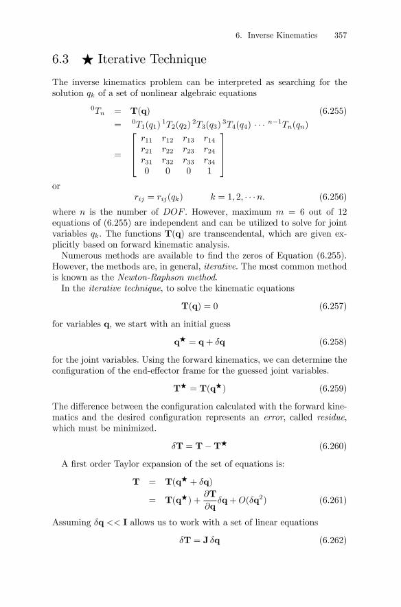
6.3 F Iterative Technique

The inverse kinematics problem can be interpreted as searching for thesolution qk of a set of nonlinear algebraic equations

0Tn = T(q) (6.255)

= 0T1(q1)1T2(q2)

2T3(q3)3T4(q4) · · · n−1Tn(qn)

=

⎡⎢⎢⎣r11 r12 r13 r14r21 r22 r23 r24r31 r32 r33 r340 0 0 1

⎤⎥⎥⎦or

rij = rij(qk) k = 1, 2, · · ·n. (6.256)

where n is the number of DOF . However, maximum m = 6 out of 12equations of (6.255) are independent and can be utilized to solve for jointvariables qk. The functions T(q) are transcendental, which are given ex-plicitly based on forward kinematic analysis.Numerous methods are available to find the zeros of Equation (6.255).

However, the methods are, in general, iterative. The most common methodis known as the Newton-Raphson method.In the iterative technique, to solve the kinematic equations

T(q) = 0 (6.257)

for variables q, we start with an initial guess

qF = q+ δq (6.258)

for the joint variables. Using the forward kinematics, we can determine theconfiguration of the end-effector frame for the guessed joint variables.

TF = T(qF) (6.259)

The difference between the configuration calculated with the forward kine-matics and the desired configuration represents an error, called residue,which must be minimized.

δT = T−TF (6.260)

A first order Taylor expansion of the set of equations is:

T = T(qF + δq)

= T(qF) +∂T

∂qδq+O(δq2) (6.261)

Assuming δq << I allows us to work with a set of linear equations

δT = J δq (6.262)


where J is the Jacobian matrix of the set of equations

J(q) =

∙∂Ti∂qj

¸(6.263)

that impliesδq = J−1 δT. (6.264)

Therefore, the unknown variables q are:

q = qF + J−1 δT (6.265)

We may use the values obtained by (6.265) as a new approximation torepeat the calculations and find newer values. Repeating the methods canbe summarized in the following iterative equation to converge to the exactvalue of the variables.

q(i+1) = q(i) + J−1(q(i)) δT(q(i)) (6.266)

This iteration technique can be set in an algorithm for easier numericalcalculations.

Algorithm 6.1. Inverse kinematics iteration technique.

1. Set the initial counter i = 0.

2. Find or guess an initial estimate q(0).

3. Calculate the residue δT(q(i)) = J(q(i)) δq(i).

If every element of T(q(i)) or its norm°°T(q(i))°° is less than a tol-

erance,°°T(q(i))°° < then terminate the iteration. The q(i) is the

desired solution.

4. Calculate q(i+1) = q(i) + J−1(q(i)) δT(q(i)).

5. Set i = i+ 1 and return to step 3 .

The tolerance can equivalently be set up on variables

q(i+1) − q(i) < (6.267)

or on JacobianJ− I < . (6.268)


Example 196 F Inverse kinematics for a 2R planar manipulator.In Example 184 we have seen that the tip point of a 2R planar manipu-

lator can be described by∙XY

¸=

∙l1cθ1 + l2c (θ1 + θ2)l1sθ1 + l2s (θ1 + θ2)

¸. (6.269)

To solve the inverse kinematics of the manipulator and find the joint coor-dinates for a known position of the tip point, we define

q =

∙θ1θ2

¸(6.270)

T =

∙XY

¸(6.271)

therefore, the Jacobian of the equations is:

J(q) =

∙∂Ti∂qj

¸=

⎡⎢⎢⎣∂X

∂θ1

∂X

∂θ2∂Y

∂θ1

∂Y

∂θ2

⎤⎥⎥⎦=

∙−l1 sin θ1 − l2 sin (θ1 + θ2) −l2 sin (θ1 + θ2)l1 cos θ1 + l2 cos (θ1 + θ2) l2 cos (θ1 + θ2)

¸(6.272)

The inverse of the Jacobian is

J−1 =−1

l1l2sθ2

∙−l2c (θ1 + θ2) −l2s (θ1 + θ2)

l1cθ1 + l2c (θ1 + θ2) l1sθ1 + l2s (θ1 + θ2)

¸(6.273)

and therefore, the iterative formula (6.266) is set up as∙θ1θ2

¸(i+1)=

∙θ1θ2

¸(i)+ J−1

Ã∙XY

¸−∙XY

¸(i)!. (6.274)

Let’s assumel1 = l2 = 1 (6.275)

T =

∙XY

¸=

∙11

¸(6.276)

and start from a guess value

q(0) =

∙θ1θ2

¸(0)=

∙π/3−π/3

¸(6.277)

for which

δT =

∙11

¸−∙cosπ/3 + cos (π/3 +−π/3)sinπ/3 + sin (π/3 +−π/3)

¸=

∙11

¸−∙

32

12

√3

¸=

∙−12

−12√3 + 1

¸. (6.278)


The Jacobian and its inverse for these values are

J =

∙−12√3 0

32 1

¸(6.279)

J−1 =

∙−23√3 0√3 1

¸(6.280)

and therefore,∙θ1θ2

¸(1)=

∙θ1θ2

¸(0)+ J−1 δT

=

∙π/3−π/3

¸+

∙−23√3 0√3 1

¸ ∙−12

−12√3 + 1

¸=

∙1.624 5−1.779 2

¸. (6.281)

Based on the iterative technique, we can find the following values andfind the solution in a few iterations.Iteration 1.

J =

∙−12√3 0

32 1

¸(6.282)

δT =

∙−12

−12√3 + 1

¸(6.283)

q(1) =

∙1.624 5−1.779 2

¸(6.284)

Iteration 2.

J =

∙−0.844 0.1540.934 0.988

¸(6.285)

δT =

∙6.516× 10−20.155 53

¸(6.286)

q(2) =

∙1.583−1.582

¸(6.287)

Iteration 3.

J =

∙−1.00 −.433× 10−3.988 .999

¸(6.288)

δT =

∙.119× 10−1−.362× 10−3

¸(6.289)

q(3) =

∙1.570795886−1.570867014

¸(6.290)


Iteration 4.

J =

∙−1.000 0.00.998 50 1.0

¸(6.291)

δT =

∙−.438× 10−6.711× 10−4

¸(6.292)

q(4) =

∙1.570796329−1.570796329

¸(6.293)

The result of the fourth iteration q(4) is close enough to the exact valueq =

£π/2 −π/2

¤T.

6.4 F Comparison of the Inverse KinematicsTechniques

6.4.1 F Existence and Uniqueness of Solution

It is clear that when the desired tool frame position 0d7 is outside theworking space of the robot, there can not be any real solution for the jointvariables of the robot. In this condition, the overall resultant of the termsunder square root signs would be negative. Furthermore, even when thetool frame position 0d7 is within the working space, there may be sometool orientations 0R7 that are not achievable without breaking joint con-straints and violating one or more joint variable limits. Therefore, existingsolutions for inverse kinematics problem generally depends on the geomet-ric configuration of the robot.The normal case is when the number of joints is six. Then, provided that

no DOF is redundant and the configuration assigned to the end-effectors ofthe robot lies within the workspace, the inverse kinematics solution exists infinite numbers. The different solutions correspond to possible configurationsto reach the same end-effector configuration.Generally speaking, when the solution of the inverse kinematics of a robot

exists, they are not unique. Multiple solutions appear because a robot canreach to a point within the working space in different configurations. Everyset of solutions is associated to a particular configuration. The elbow-upand elbow-down configuration of the 2R manipulator in Example 184 is asimple example.The multiplicity of the solution depends on the number of joints of the

manipulator and their type. The fact that a manipulator has multiple so-lutions may cause problems since the system has to be able to select oneof them. The criteria on which to base a decision may vary, but a veryreasonable choice consists of choosing the closest solution to the currentconfiguration.


When the number of joints is less than six, no solution exists unlessfreedom is reduced in the same time in the task space, for example, byconstraining the tool orientation to certain directions.When the number of joints exceeds six, the structure becomes redundant

and an infinite number of solutions exists to reach the same end-effectorconfiguration within the robot workspace. Redundancy of the robot archi-tecture is an interesting feature for systems installed in a highly constrainedenvironment. From the kinematic point of view, the difficulty lies in for-mulating the environment constraints in mathematical form, to ensure theuniqueness of the solution to the inverse kinematic problem.

6.4.2 F Inverse Kinematics Techniques

The inverse kinematics problem of robots can be solved by several meth-ods, such as decoupling, inverse transformation, iterative, screw algebra,dual matrices, dual quaternions, and geometric techniques. The decouplingand inverse transform technique using 4 × 4 homogeneous transformationmatrices suffers from the fact that the solution does not clearly indicatehow to select the appropriate solution from multiple possible solutions fora particular configuration. Thus, these techniques rely on the skills and in-tuition of the engineer. The iterative solution method often requires a vastamount of computation and moreover, it does not guarantee convergenceto the correct solution. It is especially weak when the robot is close to thesingular and degenerate configurations. The iterative solution method alsolacks a method for selecting the appropriate solution from multiple possiblesolutions.Although the set of nonlinear trigonometric equations is typically not

possible to be solved analytically, there are some robot structures that aresolvable analytically. The sufficient condition of solvability is when the 6DOF robot has three consecutive revolute joints with axes intersectingin one point. The other property of inverse kinematics is ambiguity of asolution in singular points. However, when closed-form solutions to the armequation can be found, they are seldom unique.

Example 197 F Iteration technique and n-m relationship.1− Iteration method when n = m.When the number of joint variables n is equal to the number of indepen-

dent equations generated in forward kinematics m, then provided that theJacobian matrix remains non singular, the linearized equation

δT = J δq (6.294)

has a unique set of solutions and therefore, the Newton-Raphson techniquemay be utilized to solve the inverse kinematics problem.The cost of the procedure depends on the number of iterations to be per-

formed, which depends upon different parameters such as the distance be-


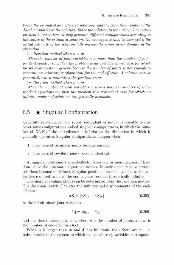
tween the estimated and effective solutions, and the condition number of theJacobian matrix at the solution. Since the solution to the inverse kinematicsproblem is not unique, it may generate different configurations according tothe choice of the estimated solution. No convergence may be observed if theinitial estimate of the solution falls outside the convergence domain of thealgorithm.2− Iteration method when n > m.When the number of joint variables n is more than the number of inde-

pendent equations m, then the problem is an overdetermined case for whichno solution exists in general because the number of joints is not enough togenerate an arbitrary configuration for the end-effector. A solution can begenerated, which minimizes the position error.3− Iteration method when n < m.When the number of joint variables n is less than the number of inde-

pendent equations m, then the problem is a redundant case for which aninfinite number of solutions are generally available.

6.5 F Singular Configuration

Generally speaking, for any robot, redundant or not, it is possible to dis-cover some configurations, called singular configurations, in which the num-ber of DOF of the end-effector is inferior to the dimension in which itgenerally operates. Singular configurations happen when:

1. Two axes of prismatic joints become parallel

2. Two axes of revolute joints become identical.

At singular positions, the end-effector loses one or more degrees of free-dom, since the kinematic equations become linearly dependent or certainsolutions become undefined. Singular positions must be avoided as the ve-locities required to move the end-effector become theoretically infinite.The singular configurations can be determined from the Jacobian matrix.

The Jacobian matrix J relates the infinitesimal displacements of the end-effector

δX = [δX1, · · · δXm] (6.295)

to the infinitesimal joint variables

δq = [δq1, · · · δqn] (6.296)

and has thus dimension m× n, where n is the number of joints, and m isthe number of end-effector DOF .When n is larger than m and J has full rank, then there are m − n

redundancies in the system to which m−n arbitrary variables correspond.


The Jacobian matrix J also determines the relationship between end-effector velocities X and joint velocities q

X = J q. (6.297)

This equation can be interpreted as a linear mapping from anm-dimensionalvector space X to an n-dimensional vector space q. The subspace R(J) isthe range space of the linear mapping, and represents all the possible end-effector velocities that can be generated by the n joints in the currentconfiguration. J has full row-rank, which means that the system does notpresent any singularity in that configuration, then the range space R(J)covers the entire vector space X. Otherwise, there exists at least one direc-tion in which the end-effector cannot be moved.The null space N(J) represents the solutions of J q = 0. Therefore, any

vector q ∈N(J) does not generate any motion for the end-effector.If the manipulator has full rank, the dimension of the null space is then

equal to the number m−n of redundant DOF . When J is degenerate, thedimension of R(J) decreases and the dimension of the null space increasesby the same amount. Therefore,

dimR(J) + dimN(J) = n. (6.298)

Configurations in which the Jacobian no longer has full rank, correspondsto singularities of the robot, which are generally of two types:

1. Workspace boundary singularities are those occurring when the ma-nipulator is fully stretched out or folded back on itself. In this case,the end effector is near or at the workspace boundary.

2. Workspace interior singularities are those occurring away from theboundary. In this case, generally two or more axes line up.

Mathematically, singularity configurations can be found by calculatingthe conditions that make

|J| = 0 (6.299)

or ¯JJT

¯= 0. (6.300)

Identification and avoidance of singularity configurations are very impor-tant in robotics. Some of the main reasons are:

1. Certain directions of motion may be unattainable.

2. Some of the joint velocities are infinite.

3. Some of the joint torques are infinite.


4. There will not exist a unique solution to the inverse kinematics prob-lem.

Detecting the singular configurations using the Jacobian determinantmay be a tedious task for complex robots. However, for robots having aspherical wrist, it is possible to split the singularity detection problem intotwo separate problems:

1. Arm singularities resulting from the motion of the manipulator arms.

2. Wrist singularities resulting from the motion of the wrist.


6.6 Summary

Inverse kinematics refers to determining the joint variables of a robot fora given position and orientation of the end-effector frame. The forwardkinematics of a 6 DOF robot generates a 4× 4 transformation matrix

0T6 = 0T11T2

2T33T4

4T55T6

=

∙0R6

0d60 1

¸=

⎡⎢⎢⎣r11 r12 r13 r14r21 r22 r23 r24r31 r32 r33 r340 0 0 1

⎤⎥⎥⎦ (6.301)

where only six elements out of the 12 elements of 0T6 are independent.Therefore, the inverse kinematics reduces to finding the six independentelements for a given 0T6 matrix.Decoupling, inverse transformation, and iterative techniques are three

applied methods for solving the inverse kinematics problem. In decouplingtechnique, the inverse kinematics of a robot with a spherical wrist can bedecoupled into two subproblems: inverse position and inverse orientationkinematics. Practically, the tools transformation matrix 0T7 is decomposedinto three submatrices 0T3, 3T6, and 6T7.

0T6 =0T3

3T66T7 (6.302)

The matrix 0T3 positions the wrist point and depends on the three manip-ulator joints’ variables. The matrix 3T6 is the wrist transformation matrixand the 6T7 is the tools transformation matrix.In inverse transformation technique, we extract equations with only one

unknown from the following matrix equations, step by step.

1T6 = 0T−110T6 (6.303)

2T6 = 1T−120T−11

0T6 (6.304)3T6 = 2T−13

1T−120T−11

0T6 (6.305)4T6 = 3T−14

2T−131T−12

0T−110T6 (6.306)

5T6 = 4T−153T−14

2T−131T−12

0T−110T6 (6.307)

I = 5T−164T−15

3T−142T−13

1T−120T−11

0T6 (6.308)

The iterative technique is a numerical method seeking to find the jointvariable vector q for a set of equations T(q) = 0.


6.7 Key Symbols

0 null vectora, b, c coefficients of trigonometric equationa turn vector of end-effector frameA local rotation transformation matrixB body coordinate framec cosd joint distancedx, dy, dz elements of dd translation vector, displacement vectordwrist wrist position vectorD displacement transformation matrixDH Denavit-HartenbergDOF degree of freedomfij the element of row i and column j of a matrixgij the element of row i and column j of a matrixG,B0 global coordinate frame, Base coordinate frameI = [I] identity matrixJ Jacobianl lengthm number of independent equationsn number of links of a robot, number of joint variablesP pointr, φ parameters of trigonometric equationr position vectors, homogeneous position vectorq joint variableq joint variables vectorri the element i of rrij the element of row i and column j of a matrixR rotation transformation matrixs sinsgn signum functionSSRMS space station remote manipulator systemT homogeneous transformation matrixTarm manipulator transformation matrixTwrist wrist transformation matrixT a set of nonlinear algebraic equations of qx, y, z local coordinate axes, local coordinatesX,Y,Z global coordinate axes, global coordinates


Greekδ Kronecker function, small increment of a parameter

small test number to terminate a procedureθ rotary joint angleθijk θi + θj + θk

Symbol[ ]−1 inverse of the matrix [ ]

[ ]T transpose of the matrix [ ]

≡ equivalent` orthogonal(i) link number ik parallel sign⊥ perpendicular× vector cross productqF a guess value for qdim dimensionN null spaceR range space


Exercises

1. Notation and symbols.

Describe the meaning of:

a- atan2 (a, b) b- 0Tn c- T(q) d- q e- J

2. 3R planar manipulator inverse kinematics.

Figure 5.21 illustrates an RkRkR planar manipulator. The forwardkinematics of the manipulator generates the following matrices. Solvethe inverse kinematics and find θ1, θ2, θ3 for given coordinates x0, y0of the tip point and a given value of ϕ.

2T3 =


⎤⎥⎥⎦

1T2 =


⎤⎥⎥⎦0T1 =


⎤⎥⎥⎦3. 2R manipulator tip point on a horizontal path.

Consider an elbow up planar 2R manipulator with l1 = l2 = 1. Thetip point is moving on a straight line from P1 (1, 1.5) to P2 (−1, 1.5).

(a) Divide the Cartesian path in 10 equal sections and determinethe joint variables at the 11 points.

(b) F Calculate the joint variable θ1 at P1 and at P2. Divide therange of θ1 into 10 equal sections and determine the coordinatesof the tip point at the 11 values of θ1.

(c) F Calculate the joint variable θ2 at P1 and at P2. Divide therange of θ1 into 10 equal sections and determine the coordinatesof the tip point at the 11 values of θ2.

4. 2R manipulator tip point on a tilted path.

Consider an elbow up planar 2R manipulator with l1 = l2 = 1. Thetip point is moving on a straight line from P1 (1, 1.5) to P2 (−1, 1).


y3y0

y1

x1

x01θ

3θ

d2

l1

z2x3

l2

x2ϕ

FIGURE 6.10. A planar manipulator.

(a) Divide the Cartesian path in 10 equal sections and determinethe joint variables at the 11 points.

(b) F Calculate the joint variable θ1 at P1 and at P2. Divide therange of θ1 into 10 equal sections and determine the coordinatesof the tip point at the 11 values of θ1.

(c) F Calculate the joint variable θ2 at P1 and at P2. Divide therange of θ1 into 10 equal sections and determine the coordinatesof the tip point at the 11 values of θ2.

5. 2R manipulator motion on a horizontal path.

Consider an elbow up planar 2R manipulator with l1 = l2 = 1. Thetip point is moving on a straight line from P1 (1, 1.5) to P2 (−1, 1.5)according to the following functions of time.

X = 1− 6t2 + 4t3 Y = 1.5

(a) Calculate and plot θ1 and θ2 as functions of time if the time ofmotion is 0 ≤ t ≤ 1.

(b) F Calculate and plot θ1 and θ2 as functions of time.

(c) F Calculate and plot θ1 and θ2 as functions of time.

(d) F Calculate and plot...θ 1 and

...θ 2 as functions of time.

6. A planar manipulator.

Figure 6.10 illustrates a three DOF planar manipulator.

(a) Determine the transformation matrices between coordinate frames.


(b) Solve the forward kinematics and determine the coordinates X,Y , and ϕ of the end-effector frame B3 for a given set of jointvariables θ1, d2, θ3.

(c) Solve the inverse kinematics and determine the joint variablesθ1, d2, θ3 for a given set of end-effector coordinates X, Y , andϕ.


Consider a planar elbow up 2R manipulator with l1 = l2 = 1. Thetip point is moving on a straight line from P1 (1, 1.5) to P2 (−1, 1.5)with a constant speed.

X = 1− vt Y = 1.5

(a) Calculate v and plot θ1 and θ2 if the time of motion is 0 ≤ t ≤ 1.(b) Calculate v and plot θ1 and θ2 if the time of motion is 0 ≤ t ≤ 5.(c) Calculate v and plot θ1 and θ2 if the time of motion is 0 ≤ t ≤ 10.(d) F Plot θ1 and θ2 as functions of v at point (0, 1.5).


Consider a planar elbow up 2R manipulator with l1 = l2 = 1. Thetip point is moving on a straight line from P1 (1, 1.5) to P2 (−1, 1.5)with a constant acceleration.

X = 1− 12at2 Y = 1.5

(a) Calculate a and plot θ1 and θ2 if the time of motion is 0 ≤ t ≤ 1.(b) Calculate a and plot θ1 and θ2 if the time of motion is 0 ≤ t ≤ 5.(c) Calculate a and plot θ1 and θ2 if the time of motion is 0 ≤ t ≤ 10.(d) F Plot θ1 and θ2 as functions of a at point (0, 1.5).

9. F 2R manipulator kinematics on a tilted path.

Consider a planar elbow up 2R manipulator with l1 = l2 = 1. Thetip point is moving on a straight line from P1 (1, 1.5) to P2 (−1, 1.5)with a constant speed.

X = 1− vt Y = 1.5

(a) Calculate and plot θ1 and θ2 if the time of motion is 0 ≤ t ≤ 1.(b) Calculate and plot θ1 and θ2 as functions of time.

(c) Calculate and plot θ1 and θ2 as functions of time.

(d) Calculate and plot...θ 1 and



10. Acceptable lengths of a 2R planar manipulator.

The tip point of a 2R planar manipulator is at (1, 1.1).

(a) Assume l1 = 1. Plot θ1 and θ2 versus l2 and determine the rangeof possible l2 for elbow up configuration.

(b) Assume l2 = 1. Plot θ1 and θ2 versus l1 and determine the rangeof possible l1 for elbow up configuration.

(c) Assume l1 = 1. Plot θ1 and θ2 versus l2 and determine the rangeof possible l2 for elbow down configuration.

(d) Assume l2 = 1. Plot θ1 and θ2 versus l1 and determine the rangeof possible l1 for elbow down configuration.

11. 3R manipulator tip point on a straight path.

Consider a 3R articulated manipulator such as Figure 6.2 with l1 =0.5, l2 = l3 = 1. The tip point is moving on a straight line fromP1 (1.5, 0, 1) to P2 (−1, 1, 1.5).

(a) Divide the Cartesian path into 10 equal sections and determinethe joint variables at the 11 points.

(b) Calculate the joint variable θ1 at P1 and at P2. Divide the rangeof θ1 into 10 equal sections and determine the coordinates of thetip point at the 11 values of θ2 and θ3.

(c) Calculate the joint variable θ2 at P1 and at P2. Divide the rangeof θ2 into 10 equal sections and determine the coordinates of thetip point at the 11 values of θ1 and θ3.

(d) Calculate the joint variable θ3 at P1 and at P2. Divide the rangeof θ3 into 10 equal sections and determine the coordinates of thetip point at the 11 values of θ1 and θ2.

12. 3R manipulator motion on a straight path.

Consider a 3R articulated manipulator such as Figure 6.2 with l1 =0.5, l2 = l3 = 1. The tip point is moving on a straight line fromP1 (1.5, 0, 1) to P2 (−1, 1, 1.5) according to the following functions oftime.

X = 1.5− 0.025t3 + 0.00375t4 − 0.00015t5

Y = 0.01t3 − 0.0015t4 + 0.00006t5

Z = 1 + 0.005t3 − 0.00075t4 + 0.00003t5

(a) Calculate and plot θ1, θ2 and θ3 if the time of motion is 0 ≤ t ≤1.

(b) F Calculate and plot θ1, θ2 and θ3 as functions of time.


X

Y

X

Y

2θ

1θ

2θ

1θ

(a) (b)

FIGURE 6.11. An elbow up 2R manipulator on a circular path.

(c) F Calculate and plot θ1, θ2 and θ3 as functions of time.

(d) F Calculate and plot...θ 1,

...θ 2 and


13. An elbow up 2R manipulator on a circular path.

The 2R manipulator of Figure 6.11 has l2 = l1 = 1. The tip point ofthe manipulator is supposed to move on a circular path with a radiusR = 1/3. Assume the manipulator starts moving when the secondlink is horizontal.

(a) Plot θ1 and θ2 if the tip point is moving counterclockwise asshown in Figure 6.11(a).

(b) Plot θ1 and θ2 if the tip point is moving clockwise as shown inFigure 6.11(b).

14. Acceptable lengths of a 3R manipulator.

The tip point of a 3R articulated manipulator is at (1, 1.1, 0.5).

(a) Assume l1 = l3 = 1. Plot θ1, θ2 and θ3 versus l2 and determinethe range of possible l2.

(b) Assume l2 = l3 = 1. Plot θ1, θ2 and θ3 versus l1 and determinethe range of possible l1.

(c) Assume l2 = l1 = 1. Plot θ1, θ2 and θ3 versus l3 and determinethe range of possible l3.

15. An elbow down 2R manipulator on a circular path.

The 2R manipulator of Figure 6.12 has l2 = l1 = 1. The tip point ofthe manipulator is supposed to move on a circular path with a radiusR = 1/3. Assume the manipulator starts moving when the first linkis horizontal.


X

Y

(a) (b)

X

Y

FIGURE 6.12. An elbow down 2R manipulator on a circular path.

X

Y2θ

1θ

FIGURE 6.13. A 2R manipulator on a circular path.

(a) Plot θ1 and θ2 if the tip point is moving counterclockwise asshown in Figure 6.12(a).

(b) Plot θ1 and θ2 if the tip point is moving clockwise as shown inFigure 6.12(b).

16. A 2R manipulator on a circular path.

The 2R manipulator of Figure 6.13 has l2 = l1 = 1. The tip point ofthe manipulator is supposed to move on a circular path with a radiusR = 4 and a center on Y -axis.

(a) Assume the elbow up manipulator starts moving on the uppercircular path when the second link is horizontal. Plot θ1 and θ2until the first link becomes horizontal at the end of the path.

(b) Assume the elbow down manipulator starts moving on the uppercircular path when the first link is horizontal. Plot θ1 and θ2 untilthe first link becomes horizontal at the end of the path.


(c) Assume the elbow up manipulator starts moving on the lowercircular path when the second link is horizontal. Plot θ1 and θ2until the first link becomes horizontal at the end of the path.

(d) Assume the elbow down manipulator starts moving on the lowercircular path when the first link is horizontal. Plot θ1 and θ2 untilthe first link becomes horizontal at the end of the path.

17. Spherical wrist inverse kinematics.

Figure 5.26 illustrates a spherical wrist with following transformationmatrices. Assume that the frame B3 is the base frame. Solve theinverse kinematics and find θ4, θ5, θ6 for a given 3T6.

3T4 =

⎡⎢⎢⎣cθ4 0 −sθ4 0sθ4 0 cθ4 00 −1 0 00 0 0 1

⎤⎥⎥⎦ 4T5 =

⎡⎢⎢⎣cθ5 0 sθ5 0sθ5 0 −cθ5 00 1 0 00 0 0 1

⎤⎥⎥⎦

5T6 =

⎡⎢⎢⎣cθ6 −sθ6 0 0sθ6 cθ6 0 00 0 1 00 0 0 1

⎤⎥⎥⎦18. F Roll-Pitch-Yaw spherical wrist kinematics.

Attach the required DH coordinate frames to the Roll-Pitch-Yawspherical wrist of Figure 5.30, similar to 5.28, and determine theforward and inverse kinematics of the wrist.

19. F Pitch-Yaw-Roll spherical wrist kinematics.

Attach the required coordinate DH frames to the Pitch-Yaw-Rollspherical wrist of Figure 5.31, similar to 5.28, and determine theforward and inverse kinematics of the wrist.

20. SCARA robot inverse kinematics.

Consider the RkRkRkP robot shown in Figure 5.23 with the followingtransformation matrices. Solve the inverse kinematics and find θ1, θ2,θ3 and d for a given 0T4.

0T1 =


⎤⎥⎥⎦

1T2 =


⎤⎥⎥⎦


2T3 =


⎤⎥⎥⎦ 3T4 =

⎡⎢⎢⎣1 0 0 00 1 0 00 0 1 d0 0 0 1

⎤⎥⎥⎦0T4 = 0T1

1T22T3

3T4

=

⎡⎢⎢⎣cθ123 −sθ123 0 l1cθ1 + l2cθ12sθ123 cθ123 0 l1sθ1 + l2sθ120 0 1 d0 0 0 1

⎤⎥⎥⎦θ123 = θ1 + θ2 + θ3 θ12 = θ1 + θ2

21. R`RkR articulated arm inverse kinematics.

Figure 5.22 illustrates 3 DOF R`RkR manipulator. Use the followingtransformation matrices and solve the inverse kinematics for θ1, θ2,θ3.

0T1 =

⎡⎢⎢⎣cos θ1 0 − sin θ1 0sin θ1 0 cos θ1 00 −1 0 d10 0 0 1

⎤⎥⎥⎦1T2 =

⎡⎢⎢⎣cos θ2 − sin θ2 0 l2 cos θ2sin θ2 cos θ2 0 l2 sin θ20 0 1 d20 0 0 1

⎤⎥⎥⎦2T3 =


⎤⎥⎥⎦22. Kinematics of a PRRR manipulator.

A PRRR manipulator is shown in Figure 6.14.

(a) Set up the links’s coordinate frame according to standard DHrules.

(b) Determine the class of each link.

(c) Find the links’ transformation matrices.

(d) Calculate the forward kinematics of the manipulator.

(e) Solve the inverse kinematics problem for the manipulator.

23. F Space station remote manipulator system inverse kinematics.

Shuttle remote manipulator system (SSRMS) is shown in Figure5.24 schematically. The forward kinematics of the robot provides the


FIGURE 6.14. A PRRR manipulator.

following transformation matrices. Solve the inverse kinematics forthe SSRMS.

0T1 =

⎡⎢⎢⎣cθ1 0 −sθ1 0sθ1 0 cθ1 00 −1 0 d10 0 0 1

⎤⎥⎥⎦ 1T2 =

⎡⎢⎢⎣cθ2 0 −sθ2 0sθ2 0 cθ2 00 −1 0 d20 0 0 1

⎤⎥⎥⎦

2T3 =

⎡⎢⎢⎣cθ3 −sθ3 0 a3cθ3sθ3 cθ3 0 a3sθ30 0 1 d30 0 0 1

⎤⎥⎥⎦ 3T4 =

⎡⎢⎢⎣cθ4 −sθ4 0 a4cθ4sθ4 cθ4 0 a4sθ40 0 1 d40 0 0 1

⎤⎥⎥⎦4T5 =

⎡⎢⎢⎣cθ5 0 sθ5 0sθ5 0 −cθ5 00 1 0 d50 0 0 1

⎤⎥⎥⎦ 5T6 =

⎡⎢⎢⎣cθ6 0 −sθ6 0sθ6 0 cθ6 00 −1 0 d60 0 0 1

⎤⎥⎥⎦6T7 =

⎡⎢⎢⎣cθ7 −sθ7 0 0sθ7 cθ7 0 00 0 1 d70 0 0 1

⎤⎥⎥⎦Hint: This robot is a one degree redundant robot. It has 7 joints whichis one more than the required 6 DOF to reach a point at a desiredorientation. To solve the inverse kinematics of this robot, we need tointroduce one extra condition among the joint variables, or assign avalue to one of the joint variables.

(a) Assume θ1 = 0 and 1T7 is given. Determine θ2, θ3, θ4, θ5, θ6, θ7.


(b) Assume θ2 = 0 and 1T7 is given. Determine θ1, θ3, θ4, θ5, θ6, θ7.

(c) Assume θ3 = 0 and 1T7 is given. Determine θ1, θ2, θ4, θ5, θ6, θ7.

(d) Assume θ5 = 0 and 1T7 is given. Determine θ1, θ2, θ3, θ4, θ6, θ7.

(e) Assume θ6 = 0 and 1T7 is given. Determine θ1, θ2, θ3, θ4, θ5, θ7.

(f) Assume θ7 = 0 and 1T7 is given. Determine θ1, θ2, θ3, θ4, θ5, θ6.

(g) Determine θ1, θ2, θ3, θ4, θ5, θ6, θ7 such that f is minimized.

f = θ1 + θ2 + θ3 + θ4 + θ5 + θ6 + θ7

6 inverse kinematics - university of minnesota duluthrlindek1/me4135_11/ch6.pdf · 6. inverse...

Documents