inverse kinematics using dynamic joint parameters: inverse
TRANSCRIPT

Vis ComputDOI 10.1007/s00371-016-1297-x
ORIGINAL ARTICLE
Inverse kinematics using dynamic joint parameters:inverse kinematics animation synthesis learnt from sub-dividedmotion micro-segments
J. Huang1 · M. Fratarcangeli2 · Y. Ding1 · C. Pelachaud1
© Springer-Verlag Berlin Heidelberg 2016
Abstract In this paper, we describe a novel parallelizablemethod for the fast computation of inverse kinematics (IK)animation. The existing IK techniques are based on sequen-tial algorithms as they compute a skeletal pose relying onlyon the previous one; However, for a given trajectory, boththe previous posture and the following posture are desiredto compute a natural posture of the current frame. Moreover,they do not take into account that the skeletal joint limits varywith temporal spatial skeleton configurations. In this paper,we describe a novel extension of IK model using dynamicjoint parameters to overcome the major drawbacks of tra-ditional approaches of IK. Our constraint model relies onmotion capture data of human motion. The dynamic jointmotion parameters are learned automatically, embeddingdynamic joint limit values and feasible poses. The joint infor-mation is stored in an octree which clusters and provides fastaccess to the data. Where the trajectory of the end-effectoris provided in the input or the target positions data are sentby data stream, all the computed poses are assembled into a
Electronic supplementary material The online version of thisarticle (doi:10.1007/s00371-016-1297-x) contains supplementarymaterial, which is available to authorized users.
B J. [email protected];[email protected]
1 CNRS LTCI and Telecom ParisTech, Paris, France
2 Chalmers University of Technology, Göteborg, Sweden
smooth animation sequence using parallel filtering and retar-geting passes. The main benefits of our approach are dual:first, the joint constraints are dynamic (as in a real humanbody), and automatically learnt from real data; second, theprocessing time is reduced significantly due to the parallelalgorithm. After describing our model, we demonstrate itsefficiency and robustness, and show that it can generate highvisual quality motion and natural looking postures with asignificant performance improvement.
Keywords Animation · Inverse kinematics · Octree ·Parallel processing
1 Introduction
Inverse kinematics (IK) uses kinematics equations to deter-mine joints’ configuration that satisfies a desired positionof an end-effector. The joints can be constrained or non-constrained. IK is widely used in robotics and computergraphics, such as motion planning and character animation.Compared to approaches reproducing animation by motioncapture (mocap) data, IK offers several advantages, includ-ing free of recording sessions, less memory space, etc. Forreal-time interaction and motion planning, IK is much moreflexible than mocap methods (Fig. 1).
Different IK methods [4,10,22,29,34,37] have been pro-posed over the last 30 years. Speed performance, precisionand stability of algorithms have been largely improved byvarious solutions [3,16,25,28,30,36].
In the past years, several algorithms have been developedto solve more specific problems as described below. Someapproaches were proposed to define IK constraints and solvethem with different priority levels [6,8,20,26,33,35,35];other works are geared towards efficient modeling of natural
123

J. Huang et al.
Fig. 1 Golf swing sequence. Top From the position of the end-effector placed on the right hand (red sphere), we compute the character’s pose infour parallel steps. Bottom Comparison between the resulting poses (wood texture) and reference mocap data (transparent red)
human poses [8,33]. To the best of our knowledge, there is noexistingwork that quantify the constraints acting on joints foranymotion types. In 3Dmodeling tools (e.g., Blender [2] andMaya [1]), the IK constraints are defined by specifying thejoint angular limits along the x , y and z axes. To create ani-mations, artists need to define these values before applyingIK. In a real human body, however, these constraints changeaccording to the particular pose.Hence, artists need tomodifythe angular values for specific poses [5,24,31]. This can be along and tedious process considering that the human skele-ton is a complex system and the joint limits have hierarchicaldependencies. Furthermore, for a same end-effector position,several solutions for the skeleton are possible (Fig. 2), eventhough, not all of them are acceptable. To achieve a desiredposture, one solution is to fix joint limits, although this mayimpair some solutions for other target positions [24].
Eventhough IK solutions are very efficient for sim-ple tasks, more complex structured tasks may significantlyimpact the computational cost. Performance boosts can beachieved by parallelizing algorithms on multi-core CPUs orGPUs. Such a process is not trivial because IK is inherentlya sequential process, i.e., each pose depends upon the previ-ous one (Fig. 3). However, if a complete trajectory of targetpositions is known, a trivial parallel IK solver would com-pute the skeletal pose for each target position independently.The resulting generated sequence would likely be discon-tinuous and would possibly not satisfy the predefined jointconstraints.Contributions This paper proposes a novel constrained IKanimation technique. Our method automatically capturesjoint motion parameters from input mocap data. The para-meters are stored in an octree and represent a model for the
Fig. 2 Different poses are obtained from the same end-effector posi-tion
dynamic nature of human joint behavior. During the anima-tion, parameters are fetched from the octree, and are usedto solve the IK problem as well as align the end-effector tothe target position. We implemented our method in a parallelpipeline to speed up the performance when the full trajec-tory of an end-effector is provided, or the target positionsare in the format of streaming data, such as real-time videogames, 3D modeling software and SAIBA-like EmbodiedConversational Agent platform [19]. All computed poses areassembled into a smooth animation sequence using paral-lel filtering and retargeting processes. Combining these twoapproaches, we show that our solution is capable of generat-ing high visual qualitymotionwith a significant performanceimprovement.
123
Inverse kinematics using dynamic joint parameters…
IK solver
p(t0)p(t1)
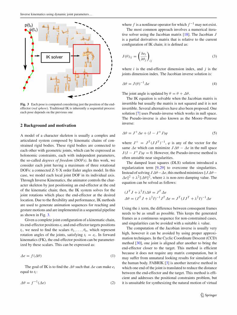
Fig. 3 Each pose is computed considering just the position of the end-effector (red sphere). Traditional IK is inherently a sequential process:each pose depends on the previous one
2 Background and motivation
A model of a character skeleton is usually a complex andarticulated system composed by kinematic chains of con-strained rigid bodies. These rigid bodies are connected toeach other with geometric joints, which can be expressed asholonomic constraints, each with independent parameters,the so-called degrees of freedom (DOFs). In this work, weconsider each joint having a maximum of three rotationalDOFs: a connected Z-Y-X order Euler angles model. In thiscase, we model each local joint DOF in its individual axis.Through Inverse Kinematics, the animator controls the char-acter skeleton by just positioning an end-effector at the endof the kinematic chain; then, the IK system solves for thejoint rotations which place the end-effector at the desiredlocation. Due to the flexibility and performance, IK methodsare used to generate animation sequences for reaching andgesturemotions and are implemented in a sequential pipelineas shown in Fig. 3.
Given a complete joint configuration of a kinematic chain,its end-effector positions ei and end-effector targets positionsti , we need to find the scalars θ1, . . . , θn , which representrotation angles of the joints, satisfying ti = ei . In forwardkinematics (FK), the end-effector position can be parameter-ized by these scalars. This can be expressed as:
Δe = f (Δθ) (1)
The goal of IK is to find the Δθ such that Δe can make eiequal to ti :
Δθ = f −1(Δe) (2)
where f is a nonlinear operator for which f −1 may not exist.The most common approach involves a numerical itera-
tive solver using the Jacobian matrix [18]. The Jacobian Jis a partial derivatives matrix that is relative to the currentconfiguration of IK chain; it is defined as:
J (θ)i j =(
∂ei∂θ j
)i j
(3)
where i is the end-effector dimension index, and j is thejoints dimension index. The Jacobian inverse solution is:
Δθ = J (θ)−1Δe (4)
The joint angle is updated by θ = θ + Δθ .The IK equation is solvable when the Jacobian matrix is
invertible but usually the matrix is not squared and it is notinvertible. Several alternatives have also been proposed. Onesolution [7] uses Pseudo-inverse which works in null space.The Pseudo-inverse is also known as the Moore–Penroseinverse:
Δθ = J+Δe + (I − J+ J )ϕ (5)
where J+ = J T (J J T )−1, ϕ is any of the vector for thesame Δe which can minimize JΔθ − Δe in the null spaceJ (I − J+ J )ϕ = 0. However, the Pseudo-inverse method isoften unstable near singularities.
The damped least squares (DLS) solution introduced aregularization term [9,29] to overcome the singularities.Instead of solving JΔθ−Δe, thismethodminimizes‖JΔθ−Δe‖2 + λ2‖Δθ‖2, where λ is non-zero damping value. Theequation can be solved as follows:
(J T J + λ2 I )Δθ = J TΔe
Δθ = (J T J + λ2 I )−1 J TΔe = J T (J J T + λ2 I )−1Δe
Using the λ term, the difference between consequent framesneeds to be as small as possible. This keeps the generatedframes as a continuous sequence for non-constrained cases,and singularities can be avoided with a suitable λ value.
The computation of the Jacobian inverse is usually veryhigh, however it can be avoided by using proper approxi-mation techniques. In the Cyclic Coordinate Descent (CCD)method [30], one joint is aligned after another to bring theend-effector closer to the target. This method is efficientbecause it does not require any matrix computation, but itmay suffer from unnatural looking results for simulation ofthe human body. FABRIK [3] is another iterative method inwhich one end of the joint is translated to reduce the distancebetween the end-effector and the target. This method is effi-cient and addresses the positional constraints problem, butit is unsuitable for synthesizing the natural motion of virtual
123

J. Huang et al.
characters. IKAN [26] is an analytic inverse kinematics sys-tem for anthropomorphic limbs; the system solves genericreaching tasks with a higher performance than conventionalJacobian systems, even though it is limited to processing asingle kinematic chain. Unfortunately, when applied to com-plete characters the results are rigid and less natural.
2.1 Related work
As early as the 1970, Liegeois et al. [21] used kinematicsequations to solve the poses of a constrained robotic armsequentially. We use a similar idea: our algorithm learns allthe parameters from input mocap data, and defines the jointlimits for each degree of freedom.
For simulating virtual characters, the result generatedusing IK solvers can be quite far from being satisfactory.
Marcelo has proposed a whole-body analytical inversekinematics (IK) method [17] which integrates collisionavoidance and customizable body control for reaching tasks.The computation is based on the interpolation of pre-designed key body postures combining with analytical IKsolution.
Mocap-based solutions have increasingly gained popular-ity because the high visual quality. Feng et al. [11] select anumber of mocap data samples that are close to the desiredconstraints, and interpolate them to obtain a new anima-tion sequence. The range of movements achievable in theirmethod is limited by the number of samples given as input.
Grochow et al. [13] use a Scaled Gaussian Process LatentVariable Model to train low dimensional IK search spacewith high-dimensional data. Their method provides an opti-mized interpolation kernel for natural poses constrained bypositional trajectories. It builds internally an interpolationplane in its motion space (or mapping space) using its vari-ance kernel, however their spatial constraints are not alwaysguaranteed to be reached. The synthesized motion variesaccording to the choice of samples, and the performancedepends on the number of sample candidates. We use a lin-ear model for small segments; the parameters are learnt byclustering similar small motion segments and this removesthe redundancy from the data.
Harish et al. [14] propose aparallel IKarchitecture for highdegree of freedom models. They also use the Damped LeastSquares Inverse Kinematics method. The parallel computa-tion is used through forward integration andposture referencefactor evaluation for differentDOFs. Their parallel solution iswell defined for high DOFs models. Their solution is appliedfor each time stamp and their scalability depends on the num-ber of DOFs, while we propose our parallel process for a totalsequence through time and our scalability depends on howlong the input trajectory is.
Our solution is not a mapping technique, but an extensionof a basic IK solver. It is able to generate natural anima-
tions by using the learnt parameters. Our solution capturesthe motion properties of the joints from input mocap data,and stores them in an octree. This octree is accessed duringthe animation to fetch the motion properties which are moresuitable for the IK solver to align the end-effector to a giventarget point. This allows us to produce natural looking posessimilar to themocap data sequence. Furthermore, we providea pipeline to compute all the poses in parallel, improving sig-nificantly the overall performance of the process.
3 Automatic learning of joint motion parameters
In our system, we employ a variation of Selective DampedLeast Squares (SDLS) IK [9,29], and we choose it as ourgeneral IK solver because of its stability near singularities.Differently from the original formulation of SDLS, we usea vector Λ = {λ1, . . . , λn}, where n is the total number ofDOFs and λi is a damping factor for the angular velocityof the i th DOF. We modify the objective function for ourdamping vector:
arg minθ∈(θmin,θmax)
‖JΔθ − Δe‖2 + ‖diag[Λ]Δθ‖2
where θmin, θmax are the boundaries ofDOFswhich are learntand stored in an octree as explained in Sect. 3.1.
The corresponding normal equation is:
(J
diag[Λ])T (
Jdiag[Λ]
)Δθ =
(J
diag[Λ])T (
Δe0
)
where diag[Λ] = ΛT I is a diagonal matrix. Hence:
Δθ =(J T J + diag
[ΛT IΛ
])−1J TΔe (6)
It is important to find a suitable assignment of values tothe minimal and maximal allowed angles for each degree offreedom, and Λ that model joint rotation velocities.
Some complex joints, such as the human shoulder, aredifficult to model manually because joint limits vary dueto muscle contraction and joint dependency [5,24,31]. Thisphenomenon inspired us to model constraints in a flexibledynamic way. Our work on constraints modeling has similargoals, but takes a different approach. We extract such valuesfrom mocap data, store them in an octree data structure anduse them during the animation.
Feng et al. [11] collect mocap data examples in a k-D tree,using K-nearest points queries to select the best candidatesequences, and blending them into the final animation. Ourwork on constraints modeling has similar goals, but takesa different approach. We use an octree data structure as acontainer and to cluster similar motions in the same cell.
123

Inverse kinematics using dynamic joint parameters…
Each cell in the octree collects similar postures data in spatialnearby region. The data in the same cell are analyzed to definethe adaptive joint constraints in this region.
3.1 Octree description
A general octree is used to cluster, compute and save ourparameter values. An octree is defined by several initial rep-resentations:The insert points Each tree point in our case represents onepose frame. All frames are sorted by the spatial 3D coordi-nates of the wrist relative to the root joint computed by theirframe poses which are the arm reaching targets (arm end-effectors) in the local space of root joint pe. A 3D positionof the wrist is actually the 3D value of an insert point.The spatial volume of octree The volume is defined by min-imum and maximum values of x , y, and z axes. Given adataset from an animation sequence, the minimum and max-imum values are decided by iterating among all insert points.The depth of octree In our tests, we use a maximum of 6levels for the octree. Mostly, the traversal level is betweenlevel 3 and level 5. The result shows the defined depth isdeep enough to get high quality motions.The tree cell (octant) An octree cell has its space subdividedin eight sub-cells. It is also a cluster of points inside of itsvolume. We keep all points (frames) in one vector. Each cellcontains the point indices corresponding to the vector. Atree cell contains parameter values computed from clusteredpoints.The insertion When a cell contains more than 20 points, wesplit the cell and put these points into the underlying level.Wedo it recursively till the maximum level. However, we do notremove the point indices in the original level. All levels have
a copy of the containing points. This is used to compute theIK parameter values for all levels and all clusters as describedin the following.
The octree is filled with mocap data in the initializationphase.We insert animation data (bvh file) by sequence. Morespecifically, each frame represents a chain pose related to thewrist position. It is also an entry point in the octree. Thisentry vi is defined as
vi ={pe; r i1, . . . , r im; i − 1
}
wherem is the number of joints degrees of freedom, pe is theend-effector position which is also the traversal index in thetree, r ij is the j th degree of freedom of the i th pose storedin the octree cell, i is the frame number and i − 1 is thecorresponding previous frame index (we can easily accessthe neighbor frame’s information in the octree). If the frameis the first frame of one sequence, we put−1 into i−1 whichindicates that the frame doesn’t have a previous frame.
Each cell of the octree stores all the indices {i1, . . . , in} ofthe entries contained in it. The motion properties of each cellare computed by using these indices to access the DOFs ofthe corresponding entries, and we can compute the minimal,maximal and weighted average values of each DOF for thecell (Fig. 4). We suppose that all the motion happening in thecell region won’t violate these DOF boundaries learnt fromdata. Taking one cell, we compute the vectors of the mini-mal and maximal values for each DOF, respectively rmin ={rmin1 , rmin
2 , . . . , rminm }, rmax = {rmax
1 , rmax2 , . . . , rmax
m }, andthe weighted average value r = {r1, r2, . . . , rm}. The angu-lar limits for the j th DOF in one cell are computed as thefollowing (see Fig. 5):
Fig. 4 aOne vertex is built by the right hand end-effector position andits skeleton posture frame; b each tree cell is filled by the data indiceswhich are used to compute its joint constraints set; c when doing ani-
mation generation, IK solver needs to traverse the octree to fetch the IKconstraints in the corresponding cell
123

J. Huang et al.
(a) (b) (c)
(d) (e) (f)
Fig. 5 Computation of rmin, rmax (red boundaries) by adding entriesin the octree cell. The shadow part is the covered range
rminj = min
(r i1j , . . . , r inj
)− ε (7)
rmaxj = max
(r i1j , . . . , r inj
)+ ε (8)
r j =∑in
i1wi
j rij∑in
i1wi
j
(9)
wij = 2π −
∣∣∣(E[r j ] − r ij
)∣∣∣ (10)
where ε is a manually set-up small arbitrary positive quantitywhich is used to control the relaxation of DOF limits whichmeans that when the original learnt joint motion range istoo small for reaching certain position, ε is used to tradeoff the reaching target constraint and joint range constraint.By default, we use 0 or 0.001 these small values to keep themotion ranges close to the original data. rmin and rmax definethe range of possible values that the DOF will have when thetarget position will traverse the cell. E[r j ] is the expectationvalue of r j which equals to the average of r i1j , . . . , r inj . Ther represents the most likely configuration in the cell amongthe observed ones.
For each entry vi in the cell, we compute also the Λi
vector. Rearranging Eq. 6:
diag[ΛT
i IΛi
]Δθ = J T (Δe − JΔθ) (11)
where Δe = pe(t) − pe(t − 1), pe(t − 1) is the position ofthe end-effector at the previous time step in the trajectory ofthe mocap data by fetching the i − 1 indexed frame entry,andΔθ = r(t)−r(t−1). We define that each couple framesi − 1 and i during Δθ is a micro-motion segment. We definethe vector g:
g = J T (Δe − JΔθ)
and compute λ2j :
λ2i j =∣∣∣∣ g j
Δθ j
∣∣∣∣
Intuitively, λ2i j represents the damping factor for the rotationof the j th DOF when the target point is in the cell. We sup-pose that eachmicro-motion segment (both start pose and thetarget pose) is in the same cell. Then, we compute the vec-tor Λ taking the average of all the Λi in the cell. Basically,we use a linear operator to find the damping factor whichis adaptable in our situation when the motion segments aresmall.
Finally, each cell in the octree contains one vector of prop-erties rmin, rmax, r,Λ. This vector represents how fast themovementwill be like and hownarrow the jointmotion rangeis in this cell region. Mostly, deeper level cells will have asmaller range for jointmotion andmore specificmotion char-acter. For the highest level, we use a set of manual set-upvalues (such as, for the elbowx axis rotation limits, rmax = 0,rmin = −3.14). Given a target point (arm wrist position), apop-up traversal process is used to find the correspondingjoint parameters in the octree. The parameters are in the cellcontaining the target point position. If an empty cell is found,wewill do a pop-up, taking a higher level cell instead, includ-ing up to the highest level. If the point is not in the tree, weuse the highest level parameters. In this case, our solutionbecomes a general SDL IK solution.
Over all, the Eq. 6 is used to solve for each frame inde-pendently. Combined with filtering kernels, we can achievea natural and smooth motion sequence. The whole processcan be computed in parallel. We explain the algorithm usingmulti-threads more clearly in the following parallel processsection.
4 Parallel computation of inverse kinematicsanimation
Given a set of target points defining a trajectory and theconstraints octree, we compute the final animation in fourparallel passes. The whole parallel pipeline is depicted inFig. 6.
Intuitively, each target point is initially assigned to a differ-ent thread, which computes the corresponding skeletal poseusing the constraint motion parameters stored in the octree.This provides a first crude approximation of the animationwhich is then refined in a smooth natural sequence in thefollowing steps, as explained in the next sections (see Fig. 7and the accompanying video for reference).
4.1 Crude IK parallel pass
In this first pass, we aim to obtain natural looking poseswithout being necessarily temporally coherent. Smoothlychanging poses in time will be obtained in the followingrefinement steps.
123

Inverse kinematics using dynamic joint parameters…
Fig. 6 Parallel pipeline of our IK framework
For each target position, the corresponding thread fetchesthe joint motion parameters from the octree and feed the IKsolver. By using the joint parameters stored in the octree,the resulting poses look natural and not synthetic, becausesuch parameters have been captured from the motion of areal human being.
For each target point, the following operations are per-formed in the corresponding thread:
1. The octree is traversed with a pop-up, finding the cell ccorresponding to the target point ti ;
2. The initial configuration of the kinematic chain isinstanced, considering θ = r, Λ = Λ, θmin = rmin,θmax = rmax (Fig. 7a).
3. The SDLS IK solver Eq. 6 is instanced to compute theskeletal configuration of the joints. A hard clamp kernelis used to cut the resulting θ into the boundary:
θ =
⎧⎪⎨⎪⎩
θmin if θ < θmin
θmax if θ > θmax
θ
(12)
Even though all the constraints are satisfied and the obtainedposes are natural looking, the obtained animation may resultas a discontinuous sequence in time, as shown in Fig. 7b andin the accompanying video.
The reason for the discontinuity is that for each smallsegment, the learnt parameters are from a small cell region.The θmin, θmax aremuch smaller than the physical joint limitsthat other referencedmethods used. The resulting angle in thesmall range may not fit for both the previous frame and thefollowing frame when each frame is computed individuallyand independently in Fig. 8. The skipped frame may happenwhen two close-frames have too much difference and theirsolutions are not sequential dependent.
Fig. 7 a Initial configuration of a kinematic chain. t0, t1 and t2 are thetarget positions along the trajectory. b Crude IK solver pass. The result-ing poses are not temporally coherent. c Temporal Alignment Filtering.The solution is now smooth but some end-effectors may be not aligned
anymore to the target position. dRetargeting and final correction. Usingthe previous solutions as the starting configuration, the IK solver finds asmooth solution with end-effectors aligned correctly to the target posi-tions. The white part is the free space for the joint’s rotation
123

J. Huang et al.
4.2 Temporal alignment filtering pass
In the second step, all the computed poses are aligned intime in a smooth, continuous sequence. We use a simple boxfilter [15,23,27], with a large half window sizew to convolvethe crude skeletal poses:
rfiltered = 1
2w
∑i∈Ω
ri (13)
where r is the joint angles configuration, Ω is the set of rin the time window, the index i is included in −w to w, andw is the size of the half window (for all our test cases, weused w = 10). At the end of this pass, the angular differencebetween corresponding joints in sequential frames is highlyreduced. As a result, the animation is temporally coherentbut the end-effectors are not guaranteed to reach the targets(Fig. 7c). In this step, we only use large window box filter toget smooth sequence which is different from the fourth step.
4.3 IK retargeting and correction passes
The remaining two parallel steps are used to further refinethe animation sequence.IK retargeting pass In this pass, we basically repeat the firststep: we instance a thread for each target position and run
Fig. 8 The possible IK results in our experience: red vertical lines areDOF ranges for each time instance learnt from the data; dot line is thesequence that each frame is generated independently; green line is thesequence with temporal alignment
the Ik solver separately for each target position. The maindifference with the first step is that the solver is fed with theresults of the previous step, in particular r andΛ. As a result,the end-effector reaches the target positions and, differentlyfrom the first step, the skeletal poses are temporally coherent(Fig. 7d).Final correction pass Even though the end-effector posi-tion and the temporal coherency are satisfied, there may becases in which the joint angular acceleration produces abruptchanges in the motion (e.g., see Figs. 9, 10).
To prevent the effect and obtain a smoother sequence, weadd another filtering pass to correct this issue. The skipped-frame problem due to the independent frame computationis solved with such a filtering process. We use a bilateralfilter [15,23,27] with a small half window size w (in thiscase w = 2 or w = 3): the weights are parameterized byboth a) the Euclidean distance between end-effector and itstarget, and b) the angular difference between frames.
rfiltered = 1
W
∑i∈Ω
ri f (‖ti − ei‖)g(‖i‖), (14)
where g is a temporal distance kernel, f is a spatial distancekernel, ti , ei are the target position and end-effector position,W is the sum of all the weights in one window. In this step,we choose to use an edge preserving filter. By using suchfilter, we can keep the sequence temporally smooth in jointspace while reducing the error in target space. We are able todeal with two signals.
For both of the f and g functions, we use aWendland [32]kernel which has derived piecewise polynomial functionswith positive definite and compact support.
wl(d) ={(
1 − dε
)4 ( 4dε
+ 1)
if 0 ≤ d ≤ ε
0 if d > ε(15)
whered is the current distance, ε is themaximumor thresholddistance. We setup the ε = w for g and ε = 0.05 for f .
Fig. 9 An example of trajectory errors in meter introduced by our method with four parallel steps. Only the second pass—aligning filter passmakes the targets unreachable (with large errors)
123

Inverse kinematics using dynamic joint parameters…
Fig. 10 Top One example of skipped frames in the retargeting pass, and this can be minimized by filtering frames in correction pass; bottom thejoints accelerations, red-line is elbow, blue-line is shoulder, the shoulder’s velocity varies too quickly
Table 1 Time performance comparison in milliseconds of differentsolutions when giving different trajectory frames (fs) from motioncapture data: sq (our sequential solution), pl (our parallelized imple-
mentation), dls1 (dls solution taking original pose as initial state), dls2(dls solution taking previous frame pose as initial state)
Motion pass sq/pl CIP 1st TAFP 2nd IKRP 3rd CFP 4th Sum
Angry sq 578.8 3.1 454.7 0.6 1037.3
1500fs pl 78.8 1.2 62.6 0.3 143.0
dls1 753.2
dls2 461.3
Throw sq 16.9 0.3 23.2 0.1 40.4
150fs pl 2.8 0.2 3.6 0.1 6.7
dls1 42.3
dls2 15.5
Move sq 110.3 1.0 50.1 0.3 161.8
600fs pl 19.9 0.6 6.1 0.3 27.0
dls1 191.3
dls2 109.4
Golf sq 265.1 3.7 200.2 0.7 469.7
2500fs pl 36.6 1.7 38.5 0.3 77.1
dls1 847.1
dls2 304.5
Tennis sq 171.0 3.7 153.1 0.6 328.4
2000fs pl 24.1 1.4 23.4 0.4 49.3
dls1 673.3
dls2 211.7
5 Results
We implemented and tested the performance of our methodon an Intel Xeon CPU @2.93GHz, 2 processors with 4cores each. The implementation uses Intel Threading Build-ing Blocks (TBB) library to parallelize the code. We testedseveral examples and report the performance in Table 1,where we compare the computational time with the sequen-tial implementation of our code. Note that the first step of thesequential implementation is equivalent to the performanceof the SDLS IK method (similar to dls2 in Table 1). Thecomputation time is not linear with the number of frames butdepends on the number of iterations needed to reach a targetposition, similarly to SDLS IK and any iterative IK method.
Table 2 The error metric of comparing different solutions with originalmocap in both joint space and target distance
Methods Joint mse Distance mse
Ours (sq/pl) 0.0015 0.00783
dls1 0.261 0.00861
dls2 0.326 0.00761
We also compute the average errors using both error metricin joint space and target distance space to evaluate differentmethods in Table 2. Our solution can generate good posturesthat are closer to the referenced mocap data compared withoriginal dls solutions.
123

J. Huang et al.
Fig. 11 Comparisonof normalizedmean squared errors (rotations overall joints) considering our animation at different levels compared to theoriginal mocap data in the example of tennis. The errors summed up for
the whole sequence are: 97.42 (level 0), 67.13 (level 1), 46.73 (level 2),34.33 (level 3), 22.22 (level 4), 12.70 (level 5)
Table 3 Time to compute an animation using octrees with differentmaximal depth
Level 0 1 2 3 4 5
Golf 227.6 92.0 75.9 78.6 77.7 76.2
Tennis 115.7 72.5 65.6 51.1 58.1 51.4
Throw 12.1 8.2 7.6 6.8 7.8 8.3
As input, we use the mocap animation sequences in theEmilya data set [12]. It turns out that the parallel version is∼7 times faster than the sequential version, and ∼ 4 timesfaster than non-constrained SDLS when a whole animationsequence is generated. It is worthmentioning that ourmethodis scalable,meaning that better performances can be achievedif more cores are available. In all the test cases, we use theright hand-wrist joint as the end-effector. To validate thesynthesized animations, we used the trajectory of the handin the original data from mocap sequences. Then, we com-pared the original ground truth (the mocap data), with ourresulting animation. This comparison is visually representedin the accompanying video. In Fig. 11, we show the nor-malized errors considering octrees with different depths. Wealso measured the performance of our method using octreeswith different maximal depths. Table 3 shows that the per-formance does not change significantly when the maximaldepth number is bigger than 2.
The effect of the smoothing process is represented inFig. 13: the smoothness of the motion is already largelyimproved after temporal alignment and retargeting. The finalfiltering step generates a continuous sequence. In extremecase, the target positions of trajectory are not in the space oflearned motion, our solution can still generate smooth ani-mation (Fig. 12) with given learned joint limits (Fig. 14).
5.1 Limitations
Our solution can generate smooth motion. However, thereexists several drawbacks. First, the input of our generationis a trajectory. Without the temporal information, it is hard
Fig. 12 Given a golf swing trajectory and tennis joint constraints, wegenerate tennis-like golf swing: top original golf, bottom tennis-likegolf
Fig. 13 Elbow joint rotation in sequential frames
to apply our filtering process. For our solution, it is requiredto stream in whole trajectories one by one to generate con-tinuous sequence. The smoothness is only guaranteed whenusing our edge preserving filters. Further, during the anima-tion the joint motion parameters are computed according tothe position of the target point: if this is not included in theoctree, the resulting animation will likely appear incoher-ent and unnatural as illustrated in the accompanying video.
123

Inverse kinematics using dynamic joint parameters…
Fig. 14 We use the octree to synthesize novel motion not present in the input mocap data
For these extreme cases, certain frames may not satisfy bothtarget constraint and DOFs limits, the trade-off parameteri-zation between constraints is needed. Moreover the filteringsteps could cut away quick joint rotation though this is a prob-lem shared by many different IK approaches. Our methoddoes not include the dimension reduction process, thus it isnot adaptable for high dimensional targets; our solution isuseful for chain IK that can generate natural postures.
6 Conclusions and future work
We propose a novel parallelizable constrained IK techniquewhich allows us tomodel and use dynamic joint motion para-meters. These values do not need to be set manually but areautomatically learned from inputmocap data. They are storedin an octree and accessed and used during the animationaccording to the current target position.
We implemented our method in a computational pipelinewhich can process in parallel all the target positions of theinput trajectory, generating smooth joint rotations and elim-inating potential discontinuities. We used SDLS IK as thebuilding block in our pipeline. However, it is noted that anyconstrained IK method can be used in our approach. Ourtechnique also allows us to parallelize the Inverse Kinemat-ics solver for temporally dependent targets in one trajectory.The parallel passes strategy can well solve the incoherentskipped-frames problem while doing multi-processing. Theobtained results show how our approach largely improves theperformance of procedural IK animation generation. Notethat this parallel strategy can be applied for different proce-dural IK methods.
As a future work, we would like to investigate theGPU-based implementation of our pipeline to speed up theperformances. We also aim to explore the idea of using aforest of octrees to characterize different types of stylistic
motion. We would also like to improve character IKs forhigh-dimensional mapping with full body performance.
References
1. Autodesk Maya (2015). http://www.autodesk.com/ Accessed 20Sept 2015
2. Blender (2015). https://www.blender.org/. Accessed 20 Sept 20153. Aristidou, A., Lasenby, J.: Fabrik: a fast, iterative solver for
the inverse kinematics problem. Graph. Models 73(5), 243–260(2011). doi:10.1016/j.gmod.2011.05.003
4. Baerlocher, P., Boulic, R.: Task-priority formulations for thekinematic control of highly redundant articulated structures. In:Proceedings of 1998 IEEE/RSJ International Conference on Intel-ligent Robots and Systems, vol. 1, pp. 323–329 (1998). doi:10.1109/IROS.1998.724639
5. Baerlocher, P., Boulic, R.: Parametrization and range of motionof the ball-and-socket joint. DEFORM/AVATARS 196, 180–190(2000)
6. Baerlocher, P., Boulic, R.: An inverse kinematics architectureenforcing an arbitrary number of strict priority levels. Vis. Comput.20(6), 402–417 (2004)
7. Baillieul, J.: Kinematic programming alternatives for redundantmanipulators. In: Proceedings of 1985 IEEE International Con-ference on Robotics and Automation, vol. 2, pp. 722–728 (1985).doi:10.1109/ROBOT.1985.1087234
8. Blow, J.: Inverse kinematics with quaternion joint limits. GameDeveloper (2002)
9. Buss, S.R., Kim, J.S.: Selectively damped least squares for inversekinematics, pp. 37–49 (2004)
10. Chiaverini, S.: Singularity-robust task-priority redundancy resolu-tion for real-time kinematic control of robot manipulators. IEEETrans. Robotics Autom. 13(3), 398–410 (1997)
11. Feng, A.W., Xu, Y., Shapiro, A.: An example-based motion syn-thesis technique for locomotion and object manipulation. In:Proceedings of the ACM SIGGRAPH Symposium on Interactive3D Graphics and Games, pp. 95–102. ACM (2012)
12. Fourati, N., Pelachaud, C.: Emilya: Emotional body expression indaily actions database, pp. 3486–3493 (2014)
13. Grochow, K., Martin, S.L., Hertzmann, A., Popovic, Z.: Style-based inverse kinematics. In: ACM SIGGRAPH 2004 Papers,SIGGRAPH ’04, pp. 522–531. ACM, New York (2004). doi:10.1145/1186562.1015755
123

J. Huang et al.
14. Harish, P., Mahmudi, M., Callennec, B.L., Boulic, R.: Parallelinverse kinematics for multithreaded architectures. ACM Trans.Graph. 35(2), 19:1–19:13 (2016)
15. Huang, J., Boubekeur, T., Ritschel, T., Holländer, M., Eisemann,E.: Separable approximation of ambient occlusion. In: Proceedingsof Eurographics 2012 Short, pp. 29–32 (2011)
16. Huang, J., Pelachaud, C.: An efficient energy transfer inverse kine-matics solution. Proc. Motion Game 2012 7660, 278–289 (2012)
17. Kallmann, M.: Analytical inverse kinematics with body posturecontrol. Comput. Anim. Virtual Worlds 19(2), 79–91 (2008)
18. Klein, C.A., Huang, C.H.: Review of pseudoinverse control for usewith kinematically redundantmanipulators. IEEETrans. Syst.ManCybern. SMC–13(2), 245–250 (1983). doi:10.1109/TSMC.1983.6313123
19. Kopp, S., Krenn, B., Marsella, S., Marshall, A.N., Pelachaud, C.,Pirker, H., Tharisson, K.R., Vilhjalmsson, H.: Towards a com-mon framework for multimodal generation in ecas: The behaviormarkup language. In: Proceedings of the 6th International Confer-ence on Intelligent Virtual Agents, pp. 21–23, Marina (2006)
20. Le Callennec, B., Boulic, R.: Interactive motion deformation withprioritized constraints. Graph. Models 68(2), 175–193 (2006)
21. Liegeois, A.: Automatic supervisory control of the configurationand behavior of multibody mechanisms. IEEE Trans. Syst. ManCybern. 7(12), 868–871 (1977)
22. Nakamura, Y., Hanafusa, H.: Inverse kinematic solutions with sin-gularity robustness for robot manipulator control. J. Dyn. Syst.Meas. Control 108(3), 163–171 (1986)
23. Paris, S., Durand, F.: A fast approximation of the bilateral filterusing a signal processing approach. In: Computer Vision—ECCV2006, pp. 568–580. Springer, Berlin (2006)
24. Shao, W., Ng-Thow-Hing, V.: A general joint component frame-work for realistic articulation in human characters. In: Proceedingsof the 2003 Symposium on Interactive 3D Graphics, pp. 11–18.ACM (2003)
25. Tang, W., Cavazza, M., Mountain, D., Earnshaw, R.A.: Real-timeinverse kinematics through constrained dynamics. In: Proceedingsof the International Workshop on Modelling and Motion CaptureTechniques for Virtual Environments, CAPTECH ’98, pp. 159–170. Springer, London (1998)
26. Tolani,D.,Goswami,A.,Badler,N.I.: Real-time inverse kinematicstechniques for anthropomorphic limbs. Graph. Models 62(5), 353–388 (2000)
27. Tomasi, C., Manduchi, R.: Bilateral filtering for gray and colorimages. In: Sixth International Conference on Computer Vision,pp. 839–846. IEEE (1998)
28. Unzueta, L., Peinado, M., Boulic, R., Suescun, A.: Full-body per-formance animation with sequential inverse kinematics. Graph.Models 70, 87–104 (2008)
29. Wampler II, C.W.: Manipulator inverse kinematic solutions basedon vector formulations and damped least-squares methods. IEEETrans. Syst. Man Cybern. 16(1), 93–101 (1986). doi:10.1109/TSMC.1986.289285
30. Wang, L.C., Chen, C.: A combined optimization method for solv-ing the inverse kinematics problems of mechanical manipulators.IEEE Trans. Robotics Autom. 7(4), 489–499 (1991). doi:10.1109/70.86079
31. Webber, B.L., Phillips, C.B., Badler, N.I.: Simulating humans:computer graphics, animation, and control, p. 68.Center forHumanModeling and Simulation (1993)
32. Wendland, H.: Piecewise polynomial, positive definite and com-pactly supported radial functions of minimal degree. Adv. Comput.Math. 4(1), 389–396 (1995)
33. Wilhelms, J., Gelder, A.V.: Fast and easy reach-cone joint limits.J. Graph. Tools 6(2), 27–41 (2001)
34. Wolovich, W., Elliott, H.: A computational technique for inversekinematics. In: The 23rd IEEE Conference on Decision and Con-trol, vol. 23, pp. 1359–1363 (1984)
35. Yamane, K., Nakamura, Y.: Naturalmotion animation through con-straining and deconstraining at will. IEEE Trans. Vis. Comput.Graph. 9, 352–360 (2003). doi:10.1109/TVCG.2003.1207443
36. Yuan, J.: Local svd inverse of robot jacobians. Robotica 19(1),79–86 (2001)
37. Zhao, J., Badler, N.I.: Inverse kinematics positioning using nonlin-ear programming for highly articulated figures.ACMTrans.Graph.13, 313–336 (1994)
J. Huang is a postdoctoralresearcher at CNRS in the lab-oratory LTCI, TELECOM Paris-Tech. His research interests aremainly interactive rendering andanimation generation with paral-lel high performance computing.He is also working on learn-ing andmodeling expressive ges-tures in interactive communica-tive system. He obtained hisPh.D. degree (2013) in computergraphics at TELECOM Paris-Tech, and received his masterdegree (2009) at University ofParis Descartes
M. Fratarcangeli is a SeniorLecturer at Chalmers Universityof Technology, in Gothenburg(Sweden). His research interestsare in the area of interactiveanimation of physically basedobjects. Previously, he was anassistant professor (2011–2014)at Sapienza University of Rome(Italy), where he also obtainedhis Ph.D. degree (2009) in thefield of computer graphics. Hehave been a visiting professor(03–07/2014) at Télécom Paris-Tech in Paris (France), and from
2004 to 2006 a visiting researcher at the Linköping Institute of Tech-nology (Sweden)
Y. Ding is a postdoctoralresearcher at CNRS in the lab-oratory LTCI, TELECOM Paris-Tech. He received the BS degree(2006) in automation from Xia-men University, the MS degree(2010) in computer science fromPierre and Marie Curie Univer-sity and the Ph.D. degree (2014)in computer science from Tele-com Paristech. His researchesinclude modeling and under-standing human communicationand interaction, with applicationin recognition and synthesis
123

Inverse kinematics using dynamic joint parameters…
C. Pelachaud is a Direc-tor of Research at CNRS inthe laboratory LTCI, TELECOMParisTech. Her research inter-est includes embodied conver-sational agent, nonverbal com-munication (face, gaze, and ges-ture), expressive behaviors andsocio-emotional agents. She isassociate editors of several jour-nals among which IEEE Trans-actions on Affective Computing,ACMTransactions on InteractiveIntelligent Systems and Journalon Multimodal User Interfaces.
She has co-edited several books on virtual agents and emotion-orientedsystems. She is recipient of the ACM—SIGAI Autonomous AgentsResearch Award 2015
123