04/18/23 Chapter 4 1

Chapter 4

Scatterplots and Correlation

04/18/23 Chapter 4 2

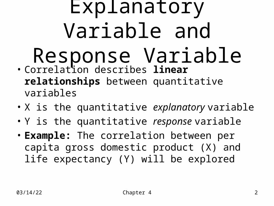
Explanatory Variable and Response Variable

• Correlation describes linear relationships between quantitative variables

• X is the quantitative explanatory variable

• Y is the quantitative response variable

• Example: The correlation between per capita gross domestic product (X) and life expectancy (Y) will be explored

04/18/23 Chapter 4 3

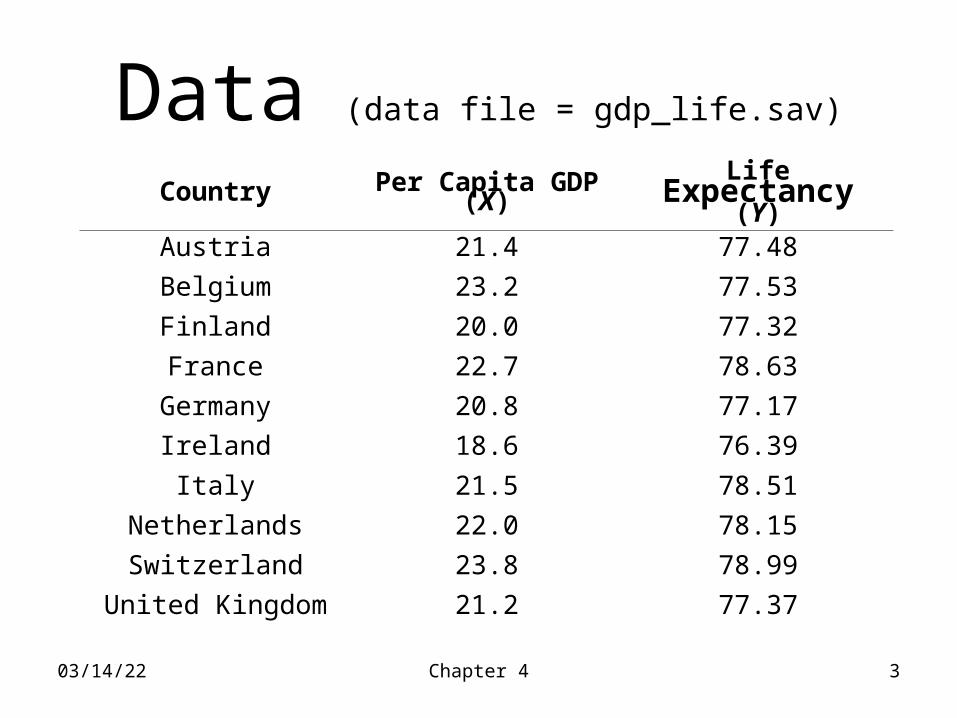
Data (data file = gdp_life.sav)

Country Per Capita GDP (X) Life Expectancy (Y)

Austria 21.4 77.48

Belgium 23.2 77.53

Finland 20.0 77.32

France 22.7 78.63

Germany 20.8 77.17

Ireland 18.6 76.39

Italy 21.5 78.51

Netherlands 22.0 78.15

Switzerland 23.8 78.99

United Kingdom 21.2 77.37

04/18/23 Chapter 4 4

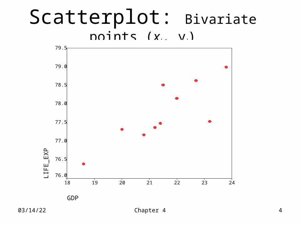
Scatterplot: Bivariate points (xi, yi)

GDP

24232221201918

LIF

E_

EX

P79.5

79.0

78.5

78.0

77.5

77.0

76.5

76.0

This is the data point for Switzerland (23.8, 78.99)

04/18/23 Chapter 4 5

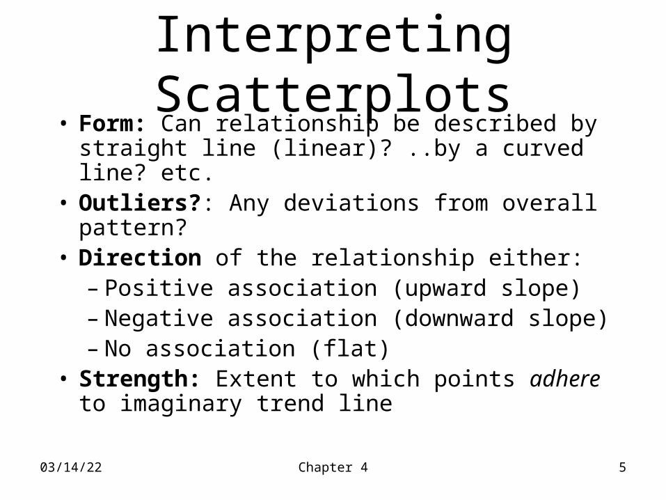
Interpreting Scatterplots• Form: Can relationship be described by

straight line (linear)? ..by a curved line? etc.• Outliers?: Any deviations from overall

pattern? • Direction of the relationship either:

– Positive association (upward slope)– Negative association (downward slope)– No association (flat)

• Strength: Extent to which points adhere to imaginary trend line

04/18/23 Chapter 4 6

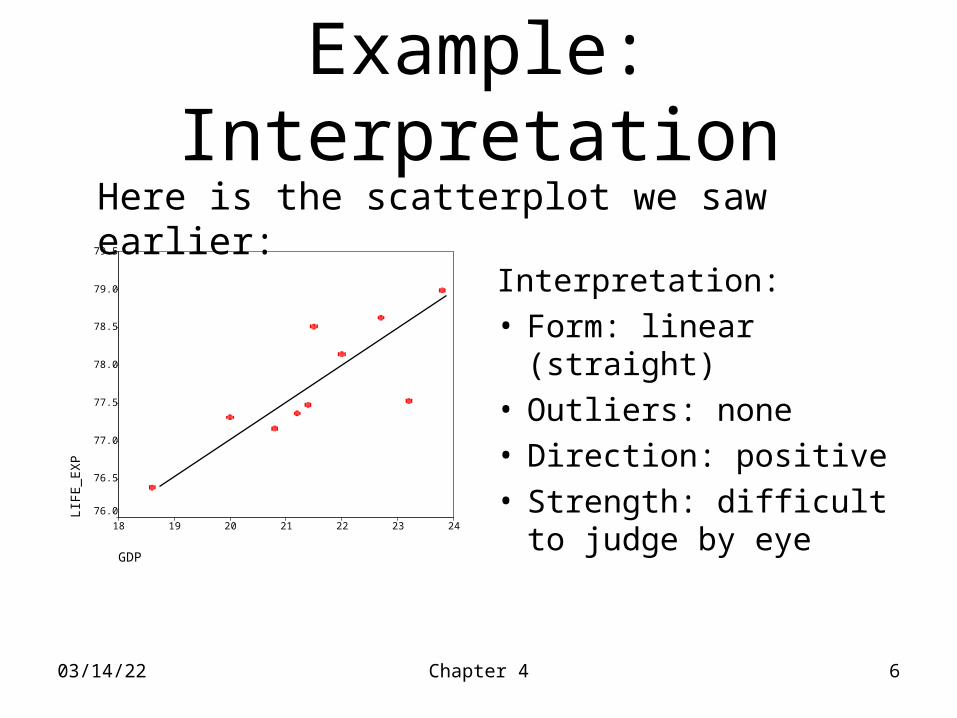
Example: Interpretation

This is the data point for Switzerland (23.8, 78.99)

GDP

24232221201918

LIF

E_

EX

P

79.5

79.0

78.5

78.0

77.5

77.0

76.5

76.0

Interpretation: • Form: linear (straight)• Outliers: none• Direction: positive• Strength: difficult to

judge by eye

Here is the scatterplot we saw earlier:

04/18/23 Chapter 4 7

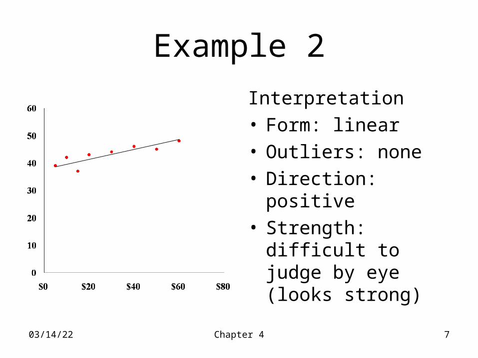
Example 2

Interpretation • Form: linear• Outliers: none• Direction: positive• Strength: difficult to

judge by eye (looks strong)

04/18/23 Chapter 4 8

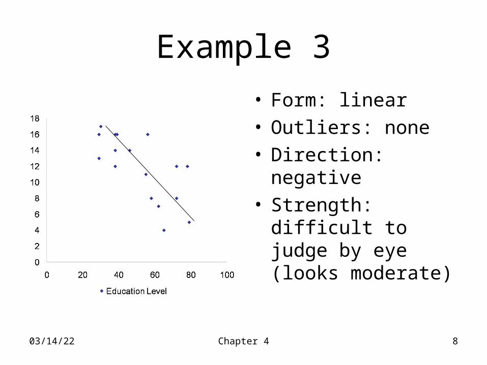
Example 3

• Form: linear• Outliers: none• Direction: negative• Strength: difficult to

judge by eye (looks moderate)

04/18/23 Chapter 4 9

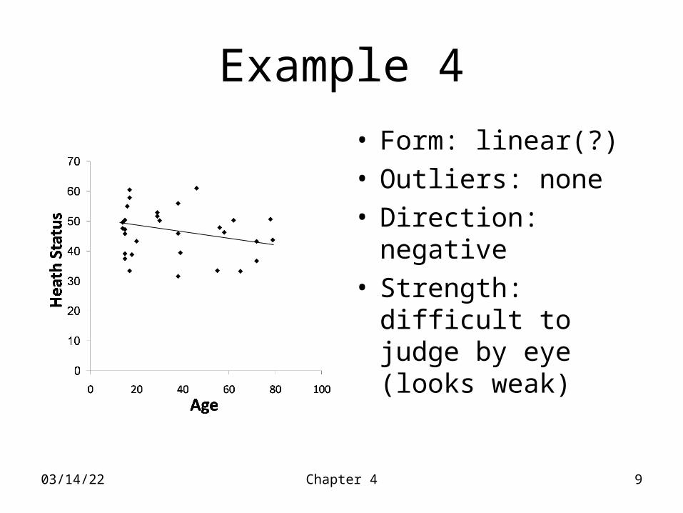
Example 4

• Form: linear(?)• Outliers: none• Direction: negative• Strength: difficult to

judge by eye (looks weak)

04/18/23 Chapter 4 10

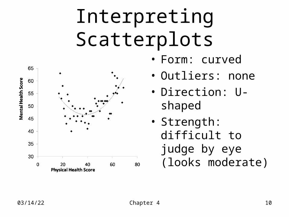
Interpreting Scatterplots

• Form: curved• Outliers: none• Direction: U-shaped• Strength: difficult to

judge by eye (looks moderate)

04/18/23 Chapter 4 11

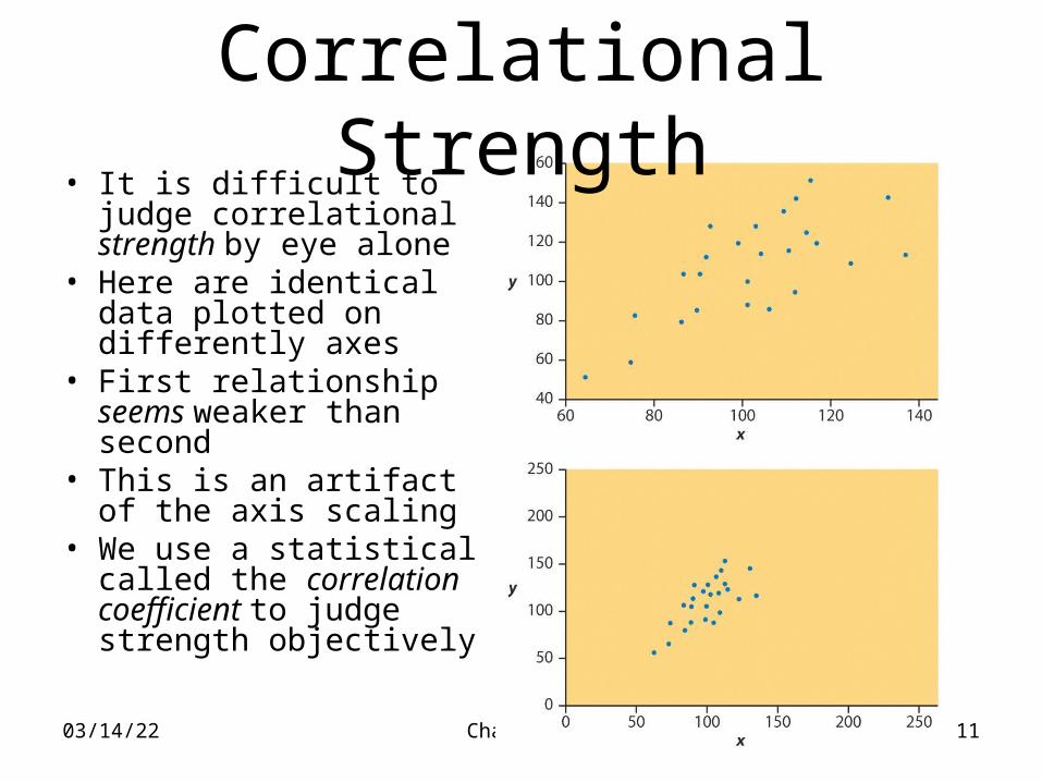
• It is difficult to judge correlational strength by eye alone

• Here are identical data plotted on differently axes

• First relationship seems weaker than second

• This is an artifact of the axis scaling

• We use a statistical called the correlation coefficient to judge strength objectively

Correlational Strength

04/18/23 Chapter 4 12

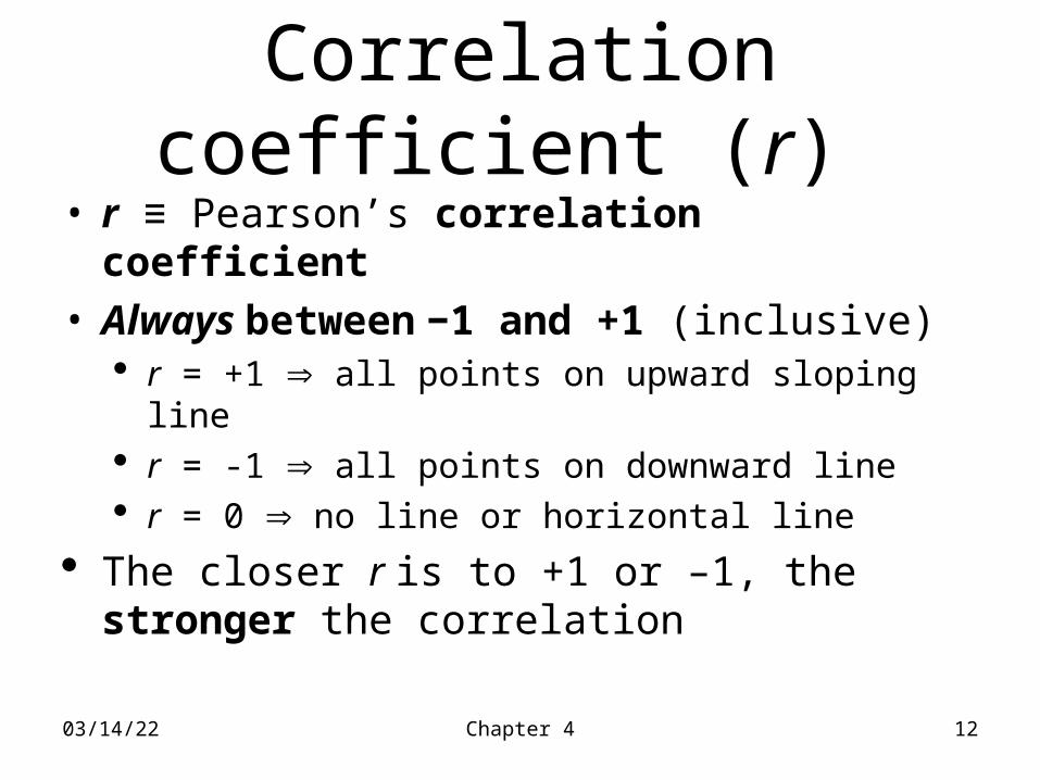
Correlation coefficient (r) • r ≡ Pearson’s correlation coefficient• Always between −1 and +1 (inclusive)

r = +1 all points on upward sloping line r = -1 all points on downward line r = 0 no line or horizontal line

The closer r is to +1 or –1, the stronger the correlation

04/18/23 Chapter 4 13

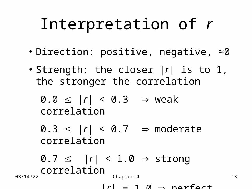
Interpretation of r

• Direction: positive, negative, ≈0

• Strength: the closer |r| is to 1, the stronger the correlation

0.0 |r| < 0.3 weak correlation

0.3 |r| < 0.7 moderate correlation

0.7 |r| < 1.0 strong correlation

|r| = 1.0 perfect correlation

04/18/23 Chapter 4 14

04/18/23 Chapter 4 15

More Examples of Correlation Coefficients

• Husband’s age / Wife’s age• r = .94 (strong positive correlation)

• Husband’s height / Wife’s height• r = .36 (weak positive correlation)

• Distance of golf putt / percent success• r = -.94 (strong negative correlation)

04/18/23 Chapter 4 16

Calculating r by hand• Calculate mean and standard deviation of X• Turn all X values into z scores• Calculate mean and standard deviation of Y• Turn all Y values into z scores• Use formula on next page

04/18/23 Chapter 4 17

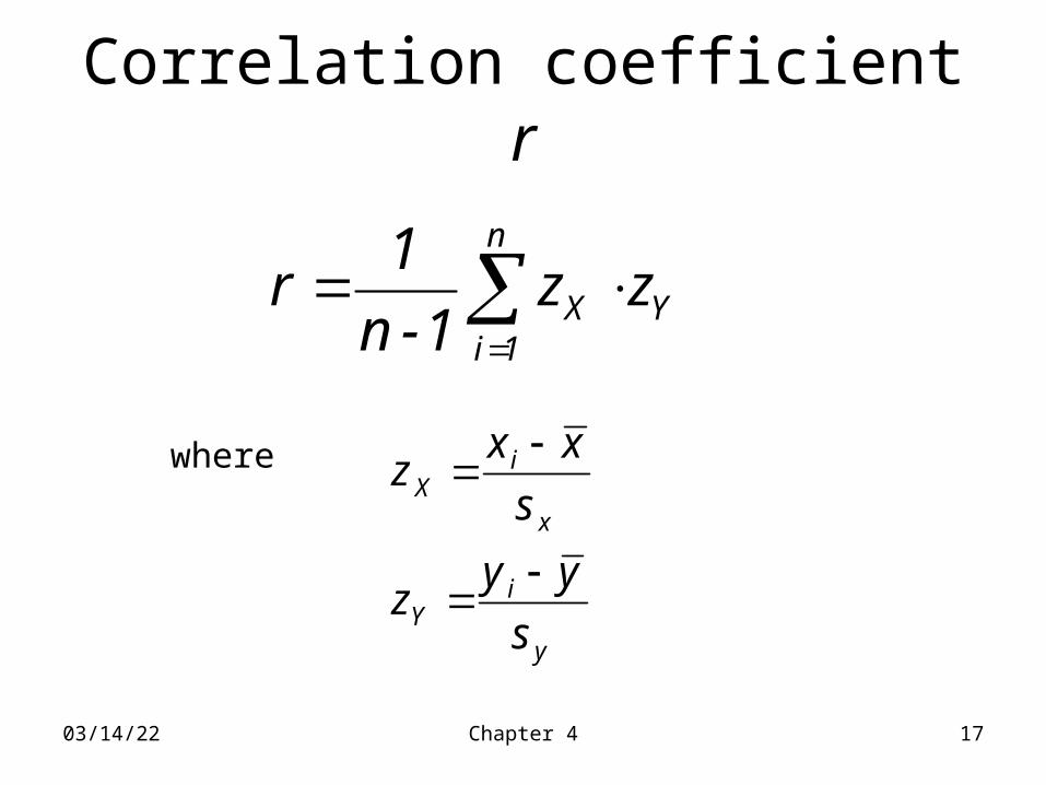
Correlation coefficient r

y

iY

x

iX

s

yyz

s

xxz

n

1i1-n

1r YX zz

where

04/18/23 Chapter 4 18

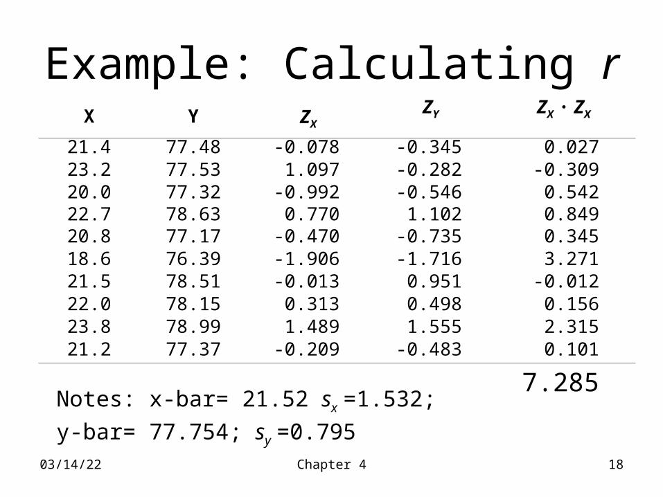
Example: Calculating rX Y ZX

ZY ZX ∙ ZX

21.4 77.48 -0.078 -0.345 0.02723.2 77.53 1.097 -0.282 -0.30920.0 77.32 -0.992 -0.546 0.54222.7 78.63 0.770 1.102 0.84920.8 77.17 -0.470 -0.735 0.34518.6 76.39 -1.906 -1.716 3.27121.5 78.51 -0.013 0.951 -0.01222.0 78.15 0.313 0.498 0.15623.8 78.99 1.489 1.555 2.31521.2 77.37 -0.209 -0.483 0.101

7.285Notes: x-bar= 21.52 sx =1.532;

y-bar= 77.754; sy =0.795

04/18/23 Chapter 4 19

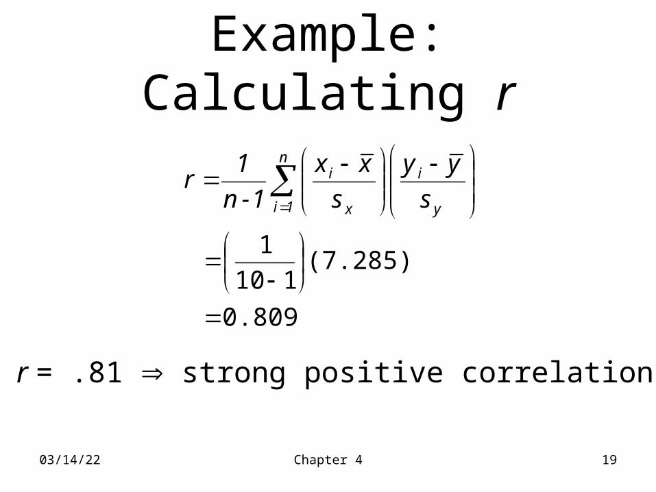
Example: Calculating r

0.809

(7.285)110

1

n

1i y

i

x

i

s

yy

s

xx

1-n

1r

r = .81 strong positive correlation

04/18/23 Chapter 4 20

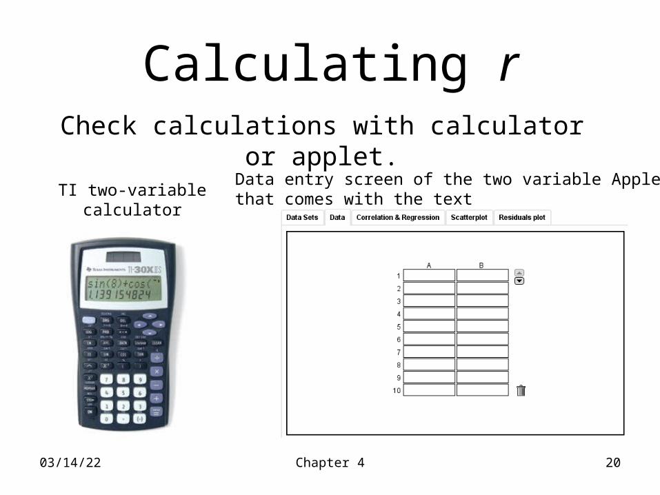
Calculating rCheck calculations with calculator or applet.

TI two-variablecalculator

Data entry screen of the two variable Appletthat comes with the text

04/18/23 Chapter 4 21

Beware!

• r applies to linear relations only

• Outliers have large influences on r

• Association does not imply causation

04/18/23 Chapter 4 22

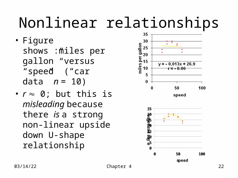
Nonlinear relationships• Figure shows :miles

per gallon” versus “speed” (“car data” n = 10)

• r 0; but this is misleading because there is a strong non-linear upside down U-shape relationship

05

1015

2025

3035

0 50 100

speed

mil

es p

er g

allo

n

04/18/23 Chapter 4 23

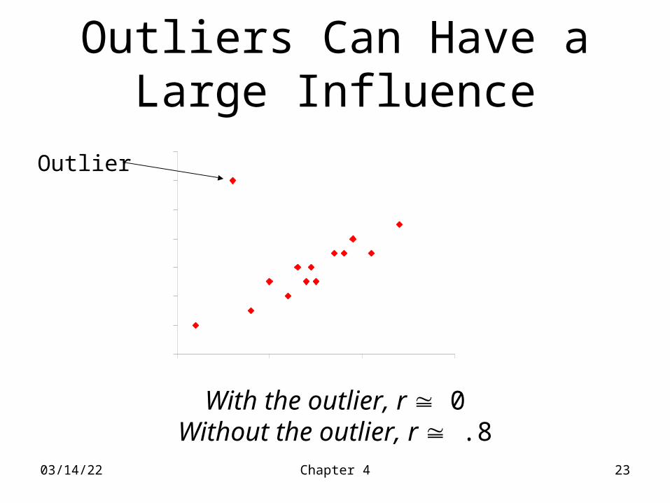
Outliers Can Have a Large Influence

With the outlier, r 0Without the outlier, r .8

Outlier

Association does not imply causation

• See text pp. 144 - 146

04/18/23 Chapter 4 25

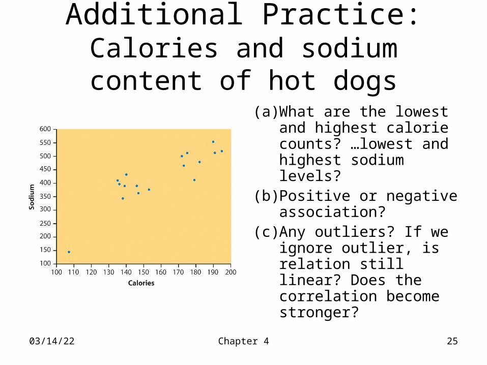
Additional Practice: Calories and sodium content of hot dogs

(a) What are the lowest and highest calorie counts? …lowest and highest sodium levels?

(b) Positive or negative association?

(c) Any outliers? If we ignore outlier, is relation still linear? Does the correlation become stronger?

04/18/23 Chapter 4 26

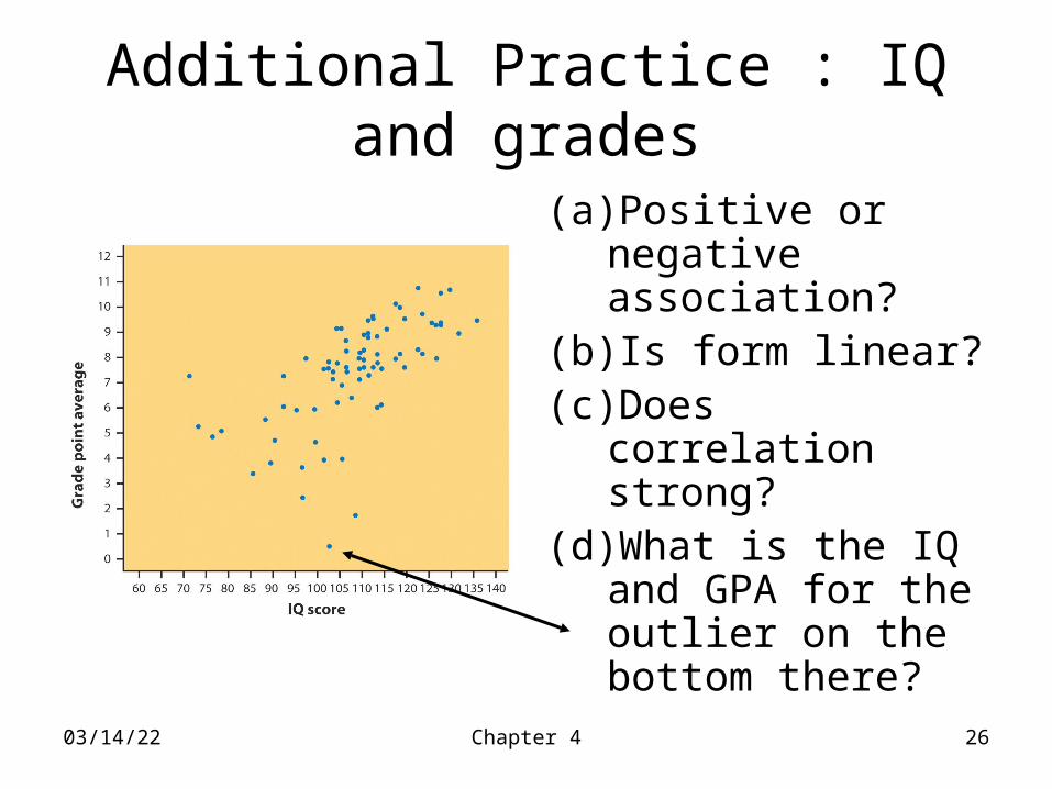
Additional Practice : IQ and grades

(a) Positive or negative association?

(b) Is form linear? (c) Does correlation

strong? (d) What is the IQ and

GPA for the outlier on the bottom there?