5erhard/downloads/textfiles/... · web viewa more abstract mathematical formulation of this...
TRANSCRIPT

Seismic Sensors and their CalibrationErhard Wielandt
5.1 OverviewThere are two basic types of seismic sensors: inertial seismometers which measure ground motion relative to an inertial reference (a suspended mass), and strainmeters or extensometers which measure the motion of one point of the ground relative to another. Since the motion of the ground relative to an inertial reference is in most cases much larger than the differential motion within a vault 9of reasonable dimensions, inertial seismometers are generally more sensitive to earthquake signals. However, at very low frequencies it becomes increasingly difficult to maintain an inertial reference, and for the observation of low-order free oscilla-tions of the Earth, tidal motions, and quasi-static deformations, strainmeters may outperform inertial seismometers. Strainmeters are conceptually simpler than inertial seismometers al-though their technical realization and installation may be more difficult (IS 5.1). This Chapter is concerned with inertial seismometers only. For a more comprehensive description of iner-tial seismometers, recorders and communication equipment see Havskov and Alguacil (2002).
An inertial seismometer converts ground motion into an electric signal but its properties can-not be described by a single scale factor, such as output volts per millimeter of ground mo-tion. The response of a seismometer to ground motion depends not only on the amplitude of the ground motion (how large it is) but also on its time scale (how sudden it is). This is be-cause the seismic mass has to be kept in place by a mechanical or electromagnetic restoring force. When the ground motion is slow, the mass will move with the rest of the instrument, and the output signal for a given ground motion will therefore be smaller. The system is thus a high-pass filter for the ground displacement. This must be taken into account when the ground motion is reconstructed from the recorded signal, and is the reason why we have to go to some length in discussing the dynamic transfer properties of seismometers.
The dynamic behavior of a seismograph system within its linear range can, like that of any linear time-invariant (LTI) system, be described with the same degree of completeness in four different ways: by a linear differential equation, the Laplace transfer function (5.2.2), the complex frequency response (5.2.3), or the impulse response of the system (5.2.4). The first two are usually obtained by a mathematical analysis of the physical system (the hardware). The latter two are directly related to certain calibration procedures (5.6.4 and 5.6.5) and can therefore be determined from calibration experiments where the system is considered as a “black box” (this is sometimes called an identification procedure). However, since all four are mathematically equivalent, we can derive each of them either from knowledge of the physical components of the system or from a calibration experiment. The mutual relations be-tween the “time-domain” and “frequency-domain” representations are illustrated in Fig. 5.1. Practically, the mathematical description of a seismometer is limited to a certain bandwidth of frequencies that should at least include the bandwidth of seismic signals. Within this limit then any of the four representations describe the system's response to arbitrary input signals completely and unambiguously. The viewpoint from which they differ is how efficiently and accurately they can be implemented in different signal-processing procedures.
- 1 -
Chapter 5: Seismic Sensors and their Calibration
In digital signal processing, seismic sensors are often represented with other methods that are efficient and accurate but not mathematically exact, such as recursive (IIR) filters. Digital signal processing is however beyond the scope of this chapter. A wealth of textbooks is avail-able both on analog and digital signal processing, for example Oppenheim and Willsky (1983) for analog processing, Oppenheim and Schafer (1975) for digital processing, and Scherbaum (1996) for seismological applications.
The most commonly used description of a seismograph response in the classical observatory practice has been the “magnification curve”, i.e. the frequency-dependent magnification of the ground motion. Mathematically this is the modulus (absolute value) of the complex fre-quency response, usually called the amplitude response. It specifies the steady-state harmonic responsivity (amplification, magnification, conversion factor) of the seismograph as a func-tion of frequency. However, for the correct interpretation of seismograms, also the phase re-sponse of the recording system must be known. It can in principle be calculated from the am-plitude response, but is normally specified separately, or derived together with the amplitude response from the mathematically more elegant description of the system by its complex transfer function or its complex frequency response.
While for a purely electrical filter it is usually clear what the amplitude response is - a dimen-sionless factor by which the amplitude of a sinusoidal input signal is multiplied - the situation is not always as clear for seismometers because different authors may prefer to measure the input signal (the ground motion) in different ways: as a displacement, a velocity, or an accel-eration. Both the physical dimension and the mathematical form of the transfer function de-pend on the definition of the input signal, and one must sometimes guess from the physical dimension to what sort of input signal it applies. The output signal, traditionally a needle de-flection, is now normally a voltage, a current, or a number of counts.
Calibrating a seismograph means measuring (and in some cases adjusting) its transfer proper-ties and expressing them as a complex frequency response or one of its mathematical equiva-lents. For most applications the result must be available as parameters of a mathematical for-mula, not as raw data, so determining parameters by fitting a theoretical curve of known shape to the data is usually part of the procedure. Practically, seismometers are calibrated in two steps.
The first step is an electrical calibration (5.6.1) in which the seismic mass is excited with an electromagnetic force. Most seismometers have a built-in calibration coil that can be con-nected to an external signal generator for this purpose. Usually the response of the system to different sinusoidal signals at frequencies across the system's passband ( 5.6.4), to impulses or steps (5.6.5), or to arbitrary broadband signals (5.6.6) is observed while the absolute mag-nification or gain remains unknown. For the exact calibration of sensors with a large dynamic range such as those employed in modern seismograph systems, the use of test signals with a broad spectrum is most appropriate. Shake tables are not suitable to measure the response of a seismometer over a large bandwidth.
The second step, the determination of the absolute gain, is more difficult because it requires mechanical test equipment in all but the simplest cases (5.6.3). The most direct method is to calibrate the seismometer on a shake table (5.6.9) or step table (5.6.10). The frequency at which the absolute gain is measured must be chosen so as to minimize noise and systematic errors, and is often predetermined by these conditions within narrow limits. Other mechanical devices such as mechanical balances and machine tools can also provide a suitable mechan-ical input for an absolute calibration (5.6.10, 5.6.11).
2
5.2 Basic theory
5.2 Basic theoryThis section introduces some basic concepts of the theory of linear systems. For a more com-plete and rigorous treatment, the reader should consult a textbook such as by Oppenheim and Willsky (1983). Digital signal processing is based on the same concepts but the mathematical formulations are different for discrete (sampled) signals (Oppenheim and Schafer, 1999, 2009); Scherbaum, 1996, 2007; Plešinger et al., 1996). Readers who are familiar with the mathematics may proceed to section 5.3.
5.2.1 The complex notationA fundamental mathematical property of linear time-invariant systems such as seismographs (as long as they are not driven out of their linear operating range) is that they do not change the waveform of sinewaves and of exponentially decaying or growing sinewaves. A more ab-stract mathematical formulation of this statement is that these waveforms are eigenfunctions of the differential operators describing LTI systems. An input signal of the form
will produce an output signal
with the same and . Note that is the angular frequency, which is times the common frequency. Using Euler’s identity
and the rules of complex algebra, we may write our input and output signals as
and
respectively, where denotes the real part and , are complex am-plitudes. It can now be seen that the only difference between the input and output signal lies in the amplitude, not in the waveform. The ratio is the complex gain of the system, and for , it is the value of the complex frequency response at the angular frequency . What we have outlined here may be called the engineering approach to complex notation. The sign
for the real part is often omitted but always understood.
The mathematical approach is slightly different in that real signals are not considered to be the real parts of complex signals but the sum of two complex-conjugate signals with positive and negative frequencies:
- 3 -

Chapter 5: Seismic Sensors and their Calibration
where the asterisk * denotes the complex conjugate. The mathematical notation is slightly less concise, but since for real signals only the term with must be explicitly written down (the other one being its complex conjugate), the two notations become very similar. How-ever, the term describes the whole signal in the engineering convention but only half of the signal in the mathematical notation! This may easily cause confusion, especially in the defini-tion of power spectra. Power spectra computed after the engineer's method (such as the USGS Low Noise Model, see 5.5.1 and Chapter 4) attribute all power to positive frequencies and therefore have twice the power appearing in the mathematical notation.
5.2.2 The Laplace transformationA signal that has a definite beginning in time (such as the seismic waves from an earthquake) can be decomposed into exponentially growing, stationary, or exponentially decaying sinu-soidal signals with the Laplace integral transformation:
,
The first integral defines the inverse transformation (the synthesis of the given signal) and the second integral the forward transformation (the analysis). It is assumed here that the signal begins at or after the time origin. s is a complex variable that may assume any value for which the second integral converges for . The Laplace transform is then said to “exist” for this value of s. The real parameter which defines the path of integration for the inverse transformation (the first integral) can be arbitrarily chosen as long as the path remains on the right side of all singularities of in the complex s plane. This parameter decides whether is synthesized from decaying ( ), stationary ( ) or growing sinu-soids. Remember that the mathematical expression with complex s represents a growing or decaying sinewave, and with imaginary s a pure sinewave.
The time derivative has the Laplace transform , the second derivative has , etc. Suppose now that an analog data-acquisition or data-processing system is char-
acterized by the linear differential equation
where is the input signal, is the output signal, and the ci and di are constants. We may then subject each term in the equation to a Laplace transformation and obtain
4
5.2 Basic theory
from which we get
We have thus expressed the Laplace transform of the output signal by the Laplace transform of the input signal, multiplied by a known rational function of s. From this we obtain the out -put signal itself by an inverse Laplace transformation. This means, we can solve the differen-tial equation by transforming it into an algebraic equation for the Laplace transforms. Of course, this is only practical if we are able to evaluate the integrals analytically, which is the case for a wide range of “mathematical” signals. Real signals must be approximated by suit-able mathematical functions for a transformation. The method can obviously be applied to linear and time-invariant differential equations of any order. (Time-invariant means that the properties of the system, and hence the coefficients of the differential equation, do not de-pend on time.)
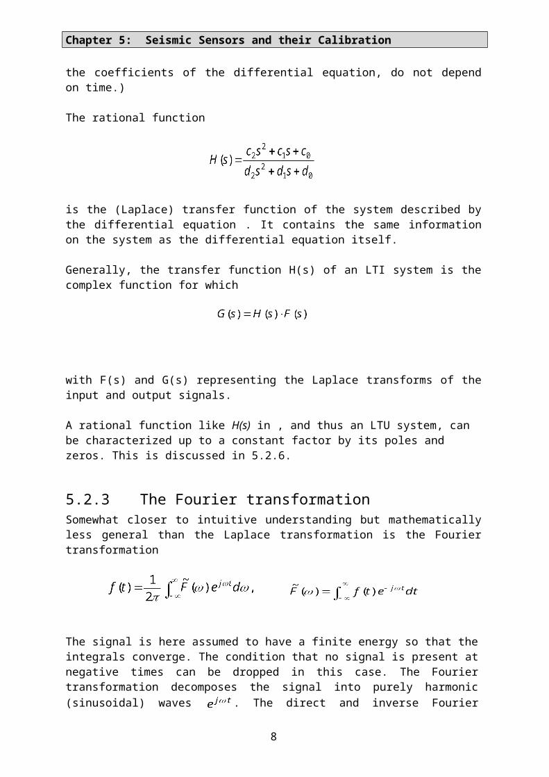
The rational function
is the (Laplace) transfer function of the system described by the differential equation . It con-tains the same information on the system as the differential equation itself.
Generally, the transfer function H(s) of an LTI system is the complex function for which
with F(s) and G(s) representing the Laplace transforms of the input and output signals.
A rational function like H(s) in , and thus an LTU system, can be characterized up to a con-stant factor by its poles and zeros. This is discussed in 5.2.6.
5.2.3 The Fourier transformationSomewhat closer to intuitive understanding but mathematically less general than the Laplace transformation is the Fourier transformation
The signal is here assumed to have a finite energy so that the integrals converge. The condi-tion that no signal is present at negative times can be dropped in this case. The Fourier trans-formation decomposes the signal into purely harmonic (sinusoidal) waves . The direct and inverse Fourier transformations are also known as a harmonic analysis and synthesis.
- 5 -
Chapter 5: Seismic Sensors and their Calibration
Although the mathematical concepts behind the Fourier and Laplace transformations are dif-ferent, we may consider the Fourier transformation as a special version of the Laplace trans-formation for real frequencies, i.e. for . In fact, by comparison with eq. , we see that
, i.e. the Fourier transform for real angular frequencies is identical to the Laplace transform for imaginary . For practical purposes the two transformations are thus nearly equivalent, and many of the relationships between time signals and their trans-forms (such as the convolution theorem) are similar or the same for both. The function is called the complex frequency response of the system. Some authors use the name “transfer function” for as well; however, is not the same function as , so a different names is appropriate. The distinction between and is essential when systems are characterized by their poles and zeros. These are equivalent but not identical in the complex s and planes, and it is important to know whether the Laplace or Fourier trans-form is meant. Usually, poles and zeros are given for the Laplace transform. In case of doubt, check the symmetry of the poles and zeros in the complex plane: those of the Laplace trans-form are symmetric to the real axis as in Figure 1 of Worksheet WS_5.7 while those of the Fourier transform are symmetric to the imaginary axis.
The absolute value is called the amplitude response, and the phase of the phase response of the system. Note that amplitude and phase do not form a symmetric pair; how-ever a certain mathematical symmetry (expressed by the Hilbert transformation) exists be-tween the real and imaginary parts of a rational transfer function, and between the phase re-sponse and the natural logarithm of the amplitude response.
The definition of the Fourier transformation according to Eq. applies to continuous transient signals. For other mathematical representations of a signal, different definitions must be used:
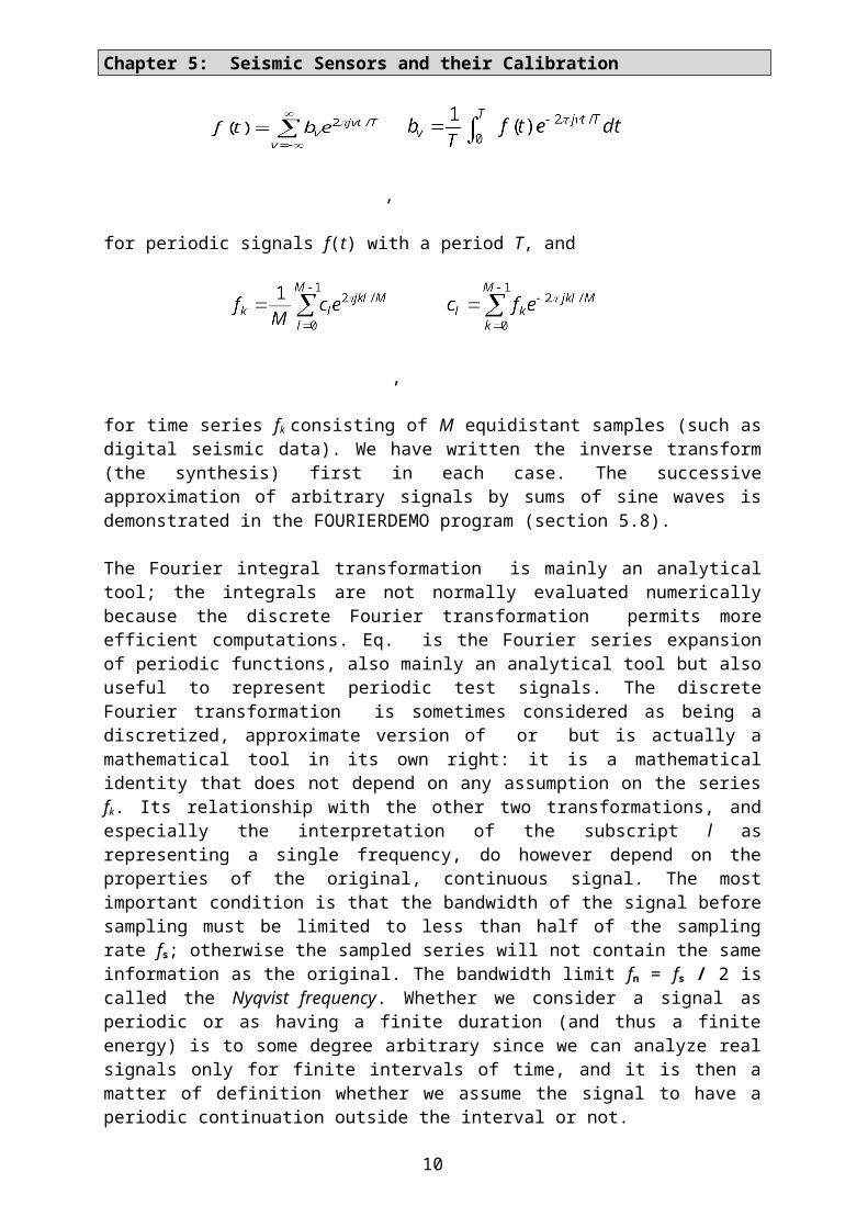
,
for periodic signals f(t) with a period T, and
,
for time series fk consisting of M equidistant samples (such as digital seismic data). We have written the inverse transform (the synthesis) first in each case. The successive approximation of arbitrary signals by sums of sine waves is demonstrated in the FOURIERDEMO program (section 5.8).
The Fourier integral transformation is mainly an analytical tool; the integrals are not nor-mally evaluated numerically because the discrete Fourier transformation permits more effi-cient computations. Eq. is the Fourier series expansion of periodic functions, also mainly an analytical tool but also useful to represent periodic test signals. The discrete Fourier transfor-mation is sometimes considered as being a discretized, approximate version of or but is ac-tually a mathematical tool in its own right: it is a mathematical identity that does not depend on any assumption on the series fk. Its relationship with the other two transformations, and es-
6

5.2 Basic theory
pecially the interpretation of the subscript l as representing a single frequency, do however depend on the properties of the original, continuous signal. The most important condition is that the bandwidth of the signal before sampling must be limited to less than half of the sam-pling rate fs; otherwise the sampled series will not contain the same information as the origi-nal. The bandwidth limit fn = fs / 2 is called the Nyqvist frequency. Whether we consider a sig-nal as periodic or as having a finite duration (and thus a finite energy) is to some degree arbi-trary since we can analyze real signals only for finite intervals of time, and it is then a matter of definition whether we assume the signal to have a periodic continuation outside the inter-val or not.
The Fast Fourier Transformation or FFT (Cooley and Tukey, 1965) is a recursive algorithm to compute the sums in efficiently, and does not constitute a mathematically different defini-tion of the discrete Fourier transformation.
5.2.4 The impulse responseA useful (although mathematically difficult) fiction is the Dirac “needle” pulse (e.g. Op-penheim and Willsky, 1983), supposed to be an infinitely short, infinitely high, positive pulse at the time origin whose integral over time equals 1. It cannot be realized, but its time-inte-gral, the unit step function, can be approximated by switching a current on or off or by sud-denly applying or removing a force. According to the definitions of the Laplace and Fourier transforms, both transforms of the Dirac pulse have the constant value 1. The amplitude spec-trum of the Dirac pulse is “white” , this means, it contains all frequencies with equal ampli -tude. In this case Eq. reduces to G(s)=H(s). The transfer function H(s) is thus the Laplace transform of the impulse response g(t). Likewise, the complex frequency response is the Fourier transform of the impulse response. All information contained in these complex func-tions is also contained in the impulse response of the system. The same is true for the step re -sponse, which is often used to test or calibrate seismic equipment.
Explicit expressions for the response of a linear system to impulses, steps, ramps and other simple waveforms can be obtained by evaluating the inverse Laplace transform over a suit-able contour in the complex s plane, provided that the poles and zeros are known. The result, generally a sum of decaying complex exponential functions (sinusoids), can then be numeri-cally evaluated with a computer or even a calculator. Although this is an elegant way of com-puting the response of a linear system to simple input signals with any desired precision, a warning is necessary: the numerical samples so obtained are not the same as the samples ob-tained with a digitizer. The digitizer must limit the bandwidth before sampling and therefore does not generate instantaneous samples but some sort of time-averages. For computing sam-ples of band-limited signals, special mathematical concepts are available (Schuessler, 1981).
Specifying the impulse or step response of a system in place of its transfer function is not practical because the analytic expressions are cumbersome to write down and represent sig-nals of infinite duration that can not be tabulated in full length.
- 7 -
Chapter 5: Seismic Sensors and their Calibration
5.2.5 The convolution theoremAny signal may be understood as consisting of a sequence of pulses. This is obvious in the case of sampled signals but can be generalized to continuous signals by representing the sig-nal as a continuous sequence of Dirac pulses. We may construct the response of a linear sys-tem to an arbitrary input signal as a sum over suitably delayed and scaled impulse responses. This process is called a convolution:
Here f(t) is the input signal and g(t) the output signal while h(t) characterizes the system. We assume that the signals are causal (i.e. zero at negative time), otherwise the integration would have to start at . Taking , i.e. using a single impulse as the input, we get
, so h(t) is in fact the impulse response of the system.
The response of a linear system to an arbitrary input signal can thus be computed either by convolution of the input signal with the impulse response in time domain, or by multiplica-tion of the Laplace-transformed input signal with the transfer function, or by multiplication of the Fourier-transformed input signal with the complex frequency response in frequency do-main.
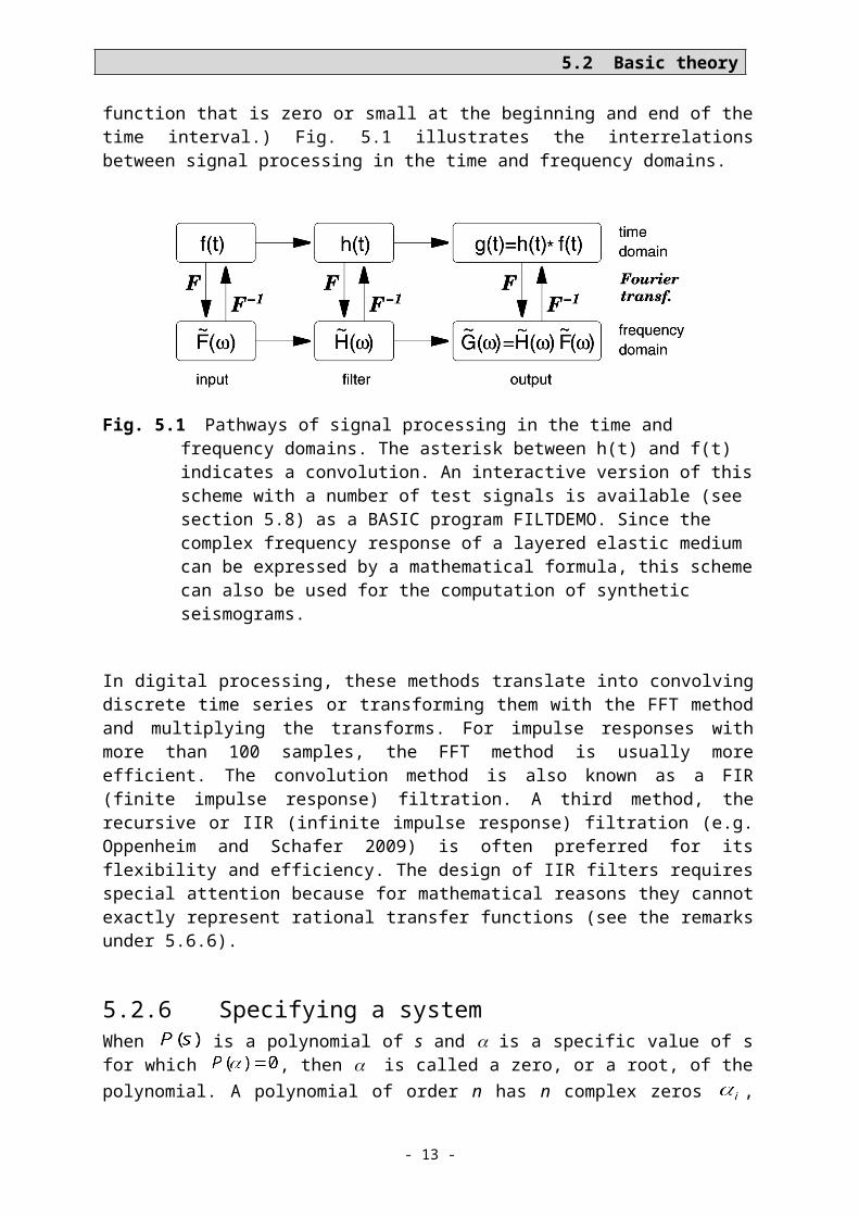
Since instrument responses are often specified as a function of frequency, the FFT algorithm has become a standard tool to compute output signals. The FFT method assumes, however, that all signals are periodic, and is therefore mathematically inaccurate when this is not the case. Signals must in general be tapered to avoid spurious results. (A taper is a weight func-tion that is zero or small at the beginning and end of the time interval.) Fig. 5.1 illustrates the interrelations between signal processing in the time and frequency domains.
Fig. 5.1 Pathways of signal processing in the time and frequency domains. The asterisk be-tween h(t) and f(t) indicates a convolution. An interactive version of this scheme with a number of test signals is available (see section 5.8) as a BASIC program FILTDEMO. Since the complex frequency response of a layered elastic medium can be expressed by a mathematical formula, this scheme can also be used for the computation of synthetic seismograms.
In digital processing, these methods translate into convolving discrete time series or trans-forming them with the FFT method and multiplying the transforms. For impulse responses
8

5.2 Basic theory
with more than 100 samples, the FFT method is usually more efficient. The convolution method is also known as a FIR (finite impulse response) filtration. A third method, the recur-sive or IIR (infinite impulse response) filtration (e.g. Oppenheim and Schafer 2009) is often preferred for its flexibility and efficiency. The design of IIR filters requires special attention because for mathematical reasons they cannot exactly represent rational transfer functions (see the remarks under 5.6.6).
5.2.6 Specifying a systemWhen is a polynomial of s and is a specific value of s for which , then is called a zero, or a root, of the polynomial. A polynomial of order n has n complex zeros , and can be factorized as .Thus, the zeros of a polynomial together with the constant p determine the polynomial completely. Since our transfer functions are ratios of two polynomials as in Eq. , they can be specified by their zeros (the zeros of the nu-merator ), their poles (the zeros of the denominator ), and a gain factor (or equiva-lently the total gain at a given frequency). The whole system, as long as it remains in its lin -ear operating range and does not produce noise, can thus be described by a small number of discrete parameters.
Transfer functions are usually specified according to one of the following concepts:
1. The real coefficients of the polynomials in the numerator and denominator are listed.
2. The denominator polynomial is decomposed into normalized first-order and second-order factors with real coefficients. (A total decomposition into first-order factors would require complex coefficients). Normally, each factor can be attributed to a specific hardware module of the system. Factors are preferably given in a form from which corner periods and damping coefficients can be read, as in Eqs. to . The numerator often reduces to a gain factor times a power of s.
3. The poles and zeros of the transfer function are listed together with a gain factor. Poles and zeros are either real or symmetric to the real axis, as mentioned above. When the nu-merator polynomial is sm, then s = 0 is an m-fold zero of the transfer function, and the sys-tem is a high-pass filter of order m. Zeros at nonzero frequency do normally not appear in the transfer function of broadband seismographs because, if they occur mathematically, their effect must practically be cancelled by nearby poles; otherwise the response would not be called broadband. Depending on the order n of the denominator and accordingly on the number of poles, the response may be flat at high frequencies (n = m), or the system may act as a low-pass filter there (n > m). The case n < m can occur only as an approxi-mation in a limited bandwidth because no practical system can have an unlimited gain at high frequencies.
In the header of the widely used SEED-format data (10.4), the gain factor is split up into a normalization factor bringing the gain to unity at a specified normalization frequency in the passband of the system, and a gain factor representing the actual gain at this frequency. EX_5.5 contains an exercise in determining the response from given poles and zeros. An in-teractive, tutorial program POLZERO in BASIC is available for this purpose (section 5.8). See also the exercises and worksheets mentioned at the end of section 5.2.
- 9 -
Chapter 5: Seismic Sensors and their Calibration
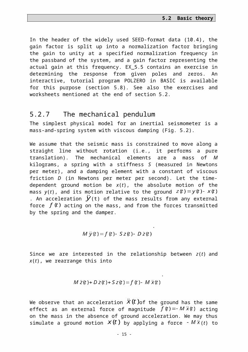
5.2.7 The mechanical pendulumThe simplest physical model for an inertial seismometer is a mass-and-spring system with viscous damping (Fig. 5.2).
We assume that the seismic mass is constrained to move along a straight line without rotation (i.e., it performs a pure translation). The mechanical elements are a mass of M kilograms, a spring with a stiffness S (measured in Newtons per meter), and a damping element with a constant of viscous friction D (in Newtons per meter per second). Let the time-dependent ground motion be x(t), the absolute motion of the mass y(t), and its motion relative to the ground . An acceleration (t) of the mass results from any external force
acting on the mass, and from the forces transmitted by the spring and the damper.
.
Since we are interested in the relationship between z(t) and x(t), we rearrange this into
.
We observe that an acceleration of the ground has the same effect as an external force of magnitude acting on the mass in the absence of ground acceleration. We may thus simulate a ground motion by applying a force (t) to the mass while the ground is not moving. The force is normally generated by sending a current through an elec-tromagnetic transducer, but it may also be applied mechanically.
Fig. 5.2 Elements of a mechanical harmonic oscillator.
5.2.8 Transfer functions of simple seismographsAccording to Eqs. and , Eq. can be rewritten as
10
5.2 Basic theory
or.
From this we can obtain directly the transfer functions Tf = Z/F for the external force F and Td
= Z/X for the ground displacement X. We arrive at the same result, expressed by the Fourier-transformed quantities, by simply assuming a time-harmonic motion as well as a time-harmonic external force , for which Eq. reduces to
or.
In mathematical derivations it is convenient to use the angular frequency = 2 f to describe a sinusoidal signal of frequency f. Some authors omit the word „angular“ in this context; we will however reserve the term „frequency“ for the number of cycles per second.
By checking the behavior of in the limit of low and high frequencies, we find that the mass-and-spring system is a second-order high-pass filter for displacements and a second-or-der low-pass filter for accelerations and external forces (Fig. 5.3). Its corner frequency is fo=o/2 with 0 = . This is at the same time the „eigenfrequency“ or „natural fre-quency“ with which the mass oscillates when the damping is negligible. At the angular fre-quency 0 , the ground motion is amplified by a factor 0 M/D and phase shifted by /2. The imaginary term in the denominator is usually written as where is the numerical damping, i.e., the ratio of the actual to the critical damping.
In order to convert the motion of the mass into an electric signal, the mechanical pendulum in the simplest case is equipped with an electromagnetic velocity transducer (5.3.8) whose out-put voltage we denote with . We then have an electromagnetic seismometer (or geophone when designed for seismic exploration). When the responsivity of the transducer is E (volts per meter per second; ) we get
from which, in the absence of an external force (i.e. , ), we obtain the frequency-dependent complex response functions
for the displacement,
- 11 -
Chapter 5: Seismic Sensors and their Calibration
for the velocity, and
for the acceleration.
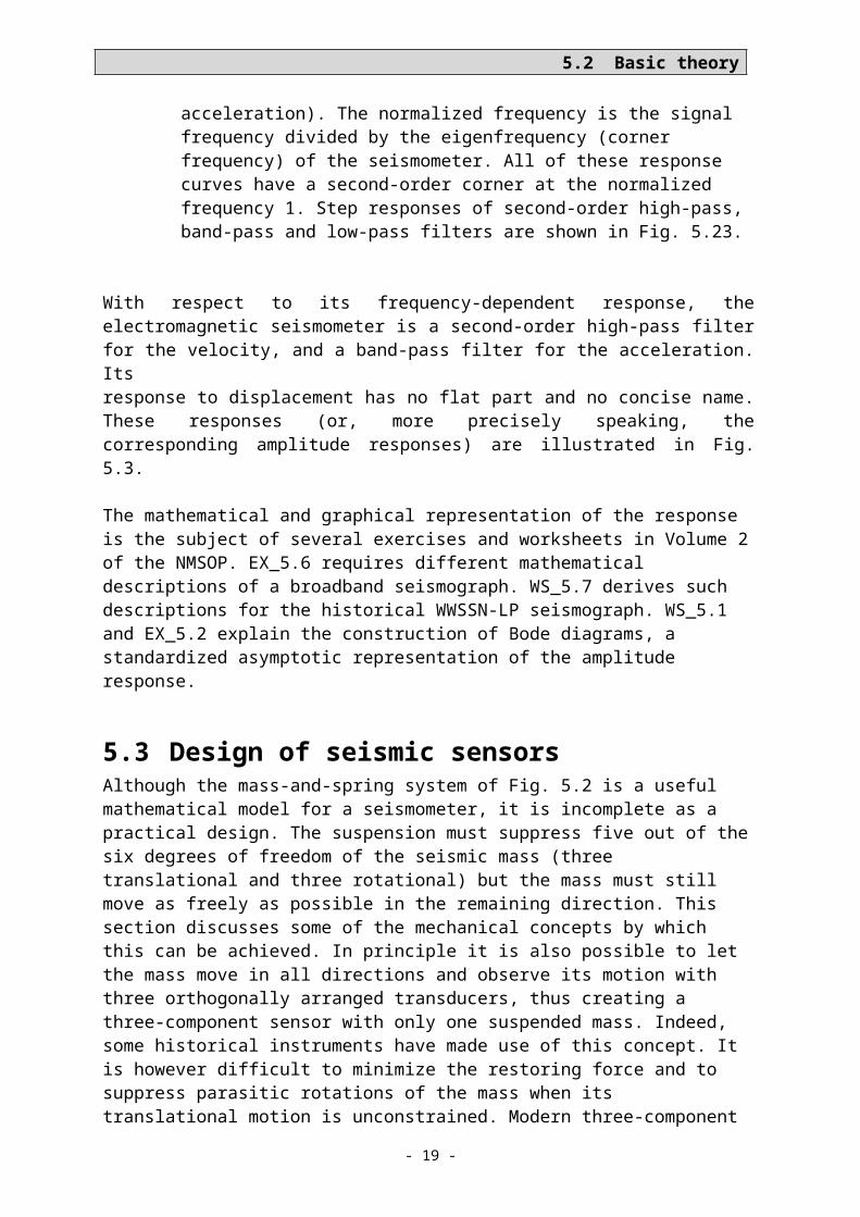
Fig. 5.3 Response curves of a mechanical seismometer (spring pendulum, left) and electro-dynamic seismometer (geophone, right) with respect to different kinds of input signals (displacement, velocity, and acceleration). The normalized frequency is the signal frequency divided by the eigenfrequency (corner frequency) of the seis-mometer. All of these response curves have a second-order corner at the normal-ized frequency 1. Step responses of second-order high-pass, band-pass and low-pass filters are shown in Fig. 5.23.
12
5.2 Basic theory
With respect to its frequency-dependent response, the electromagnetic seismometer is a sec-ond-order high-pass filter for the velocity, and a band-pass filter for the acceleration. Its response to displacement has no flat part and no concise name. These responses (or, more precisely speaking, the corresponding amplitude responses) are illustrated in Fig. 5.3.
The mathematical and graphical representation of the response is the subject of several exer-cises and worksheets in Volume 2 of the NMSOP. EX_5.6 requires different mathematical descriptions of a broadband seismograph. WS_5.7 derives such descriptions for the historical WWSSN-LP seismograph. WS_5.1 and EX_5.2 explain the construction of Bode diagrams, a standardized asymptotic representation of the amplitude response.
5.3 Design of seismic sensorsAlthough the mass-and-spring system of Fig. 5.2 is a useful mathematical model for a seis-mometer, it is incomplete as a practical design. The suspension must suppress five out of the six degrees of freedom of the seismic mass (three translational and three rotational) but the mass must still move as freely as possible in the remaining direction. This section discusses some of the mechanical concepts by which this can be achieved. In principle it is also possi-ble to let the mass move in all directions and observe its motion with three orthogonally ar-ranged transducers, thus creating a three-component sensor with only one suspended mass. Indeed, some historical instruments have made use of this concept. It is however difficult to minimize the restoring force and to suppress parasitic rotations of the mass when its transla-tional motion is unconstrained. Modern three-component seismometers therefore have sepa-rate mechanical sensors for the three axes of motion.
5.3.1 Pendulum-type seismometersMost seismometers are of the pendulum type, i.e., they let the mass rotate around an axis rather than move along a straight line (Fig. 5.4 to Fig. 5.7). The point bearings in our figures are for illustration only; most seismometers have crossed flexural hinges. Pendulums are not only sensitive to translational but also to angular acceleration. Forbriger (2009) shows how-ever that this sensitivity depends on an arbitrary definition. In order to decompose the motion of the pendulum into a translational and a rotational part, we must define an axis of rotation. When it is properly chosen, the rotational sensitivity disappears. The rotational component of seismic signals is normally so small that there is no practical difference between linear-mo-tion and pendulum-type seismometers.
Fig. 5.4 (a) Garden-gate suspension; (b) Inverted pendulum.
- 13 -
Chapter 5: Seismic Sensors and their Calibration
For small translational ground motions the equation of motion of a pendulum is formally identical to Eq. but z must then be interpreted as the angle of rotation. Since the rotational counterparts of the constants M, R, and S in Eq. are of little interest in modern electronic seismometers, we will not discuss them further and refer the reader instead to the older litera-ture, such as Berlage (1932) or Willmore (1979).
The simplest example of a pendulum is a mass suspended with a string or wire (like Fou-cault’s pendulum). When the mass has small dimensions compared to the length of the string so that it can be idealized as a point mass, then the arrangement is called a mathemati-cal pendulum. Its period of oscillation is where g is the gravitational accelera-tion. A mathematical pendulum of 1 m length has a period of nearly 2 seconds; for a period of 20 seconds the length is 100 m. Clearly, this is not a suitable design for a long-period seis-mometer.
5.3.2 Decreasing the restoring forceAt low frequencies and in the absence of an external force, Eq. can be simplified to
and read as follows: A relative displacement of the seismic mass indicates a ground acceleration
where is the angular eigenfrequency of the pendulum, and T0 its eigenperiod. If is the smallest mechanical displacement that can be detected electronically, then the formula de-termines the smallest ground acceleration that can be observed at low frequencies. For a given transducer, it is inversely proportional to the square of the free period of the suspen-sion. A sensitive long-period seismometer therefore requires either a pendulum with a low eigenfrequency or a very sensitive transducer. Since the eigenfrequency of an ordinary pen-dulum is essentially determined by its size, and seismometers must be reasonably small, astatic suspensions have been invented that combine small overall size with a long free pe-riod.
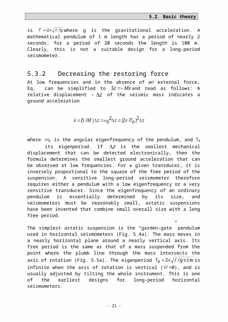
The simplest astatic suspension is the “garden-gate” pendulum used in horizontal seismome-ters (Fig. 5.4a). The mass moves in a nearly horizontal plane around a nearly vertical axis. Its free period is the same as that of a mass suspended from the point where the plumb line through the mass intersects the axis of rotation (Fig. 5.5a). The eigenperiod
is infinite when the axis of rotation is vertical ( =0), and is usually ad-justed by tilting the whole instrument. This is one of the earliest designs for long-period hori-zontal seismometers.
14
5.2 Basic theory
Fig. 5.5 Equivalence between a tilted “garden-gate” pendulum and a string pendulum. For a free period of 20 sec, the string pendulum must be 100 m long. The tilt angle of a garden-gate pendulum with the same free period and a length of 30 cm is about 0.2°. The longer the period is made, the less stable it will be under the influ-ence of small tilt changes. (b) Period-lengthening with an auxiliary compressed spring.
Another early design is the inverted pendulum held in stable equilibrium by springs or by a stiff hinge (Fig. 5.4b); a famous example is Wiechert's horizontal pendulum built around 1905.
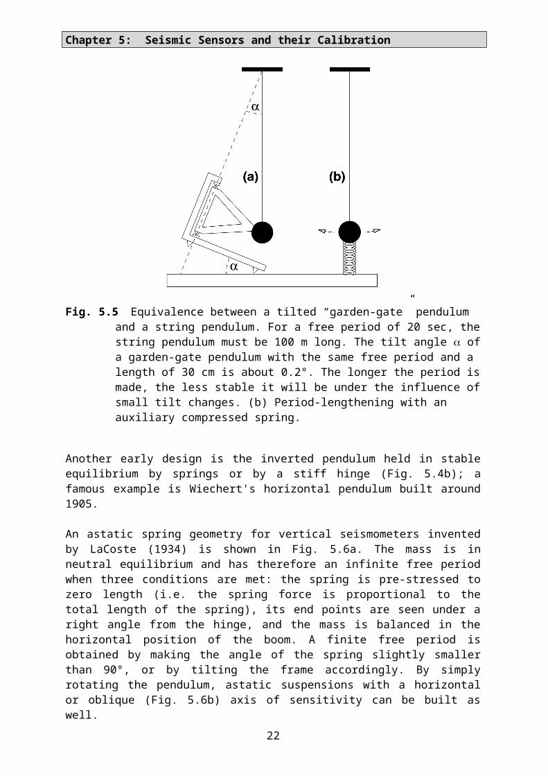
An astatic spring geometry for vertical seismometers invented by LaCoste (1934) is shown in Fig. 5.6a. The mass is in neutral equilibrium and has therefore an infinite free period when three conditions are met: the spring is pre-stressed to zero length (i.e. the spring force is pro-portional to the total length of the spring), its end points are seen under a right angle from the hinge, and the mass is balanced in the horizontal position of the boom. A finite free period is obtained by making the angle of the spring slightly smaller than 90°, or by tilting the frame accordingly. By simply rotating the pendulum, astatic suspensions with a horizontal or oblique (Fig. 5.6b) axis of sensitivity can be built as well.
Fig. 5.6 LaCoste suspensions.
- 15 -

Chapter 5: Seismic Sensors and their Calibration
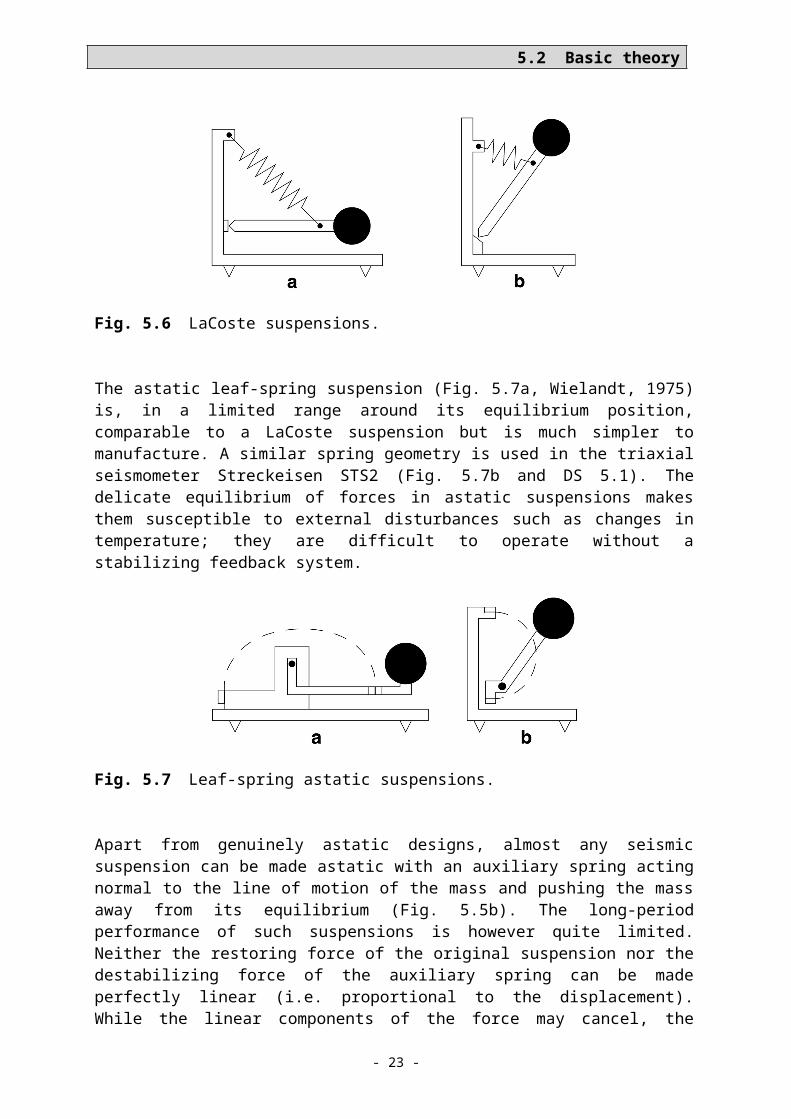
The astatic leaf-spring suspension (Fig. 5.7a, Wielandt, 1975) is, in a limited range around its equilibrium position, comparable to a LaCoste suspension but is much simpler to manufac-ture. A similar spring geometry is used in the triaxial seismometer Streckeisen STS2 (Fig.5.7b and DS 5.1). The delicate equilibrium of forces in astatic suspensions makes them sus-ceptible to external disturbances such as changes in temperature; they are difficult to operate without a stabilizing feedback system.
Fig. 5.7 Leaf-spring astatic suspensions.
Apart from genuinely astatic designs, almost any seismic suspension can be made astatic with an auxiliary spring acting normal to the line of motion of the mass and pushing the mass away from its equilibrium (Fig. 5.5b). The long-period performance of such suspensions is however quite limited. Neither the restoring force of the original suspension nor the destabil-izing force of the auxiliary spring can be made perfectly linear (i.e. proportional to the dis-placement). While the linear components of the force may cancel, the nonlinear terms remain and cause the oscillation to become non-harmonic and even unstable at large amplitudes. Vis-cous and hysteretic behaviour of the springs may also become noticeable. The additional spring (which has to be soft) may introduce a parasitic resonance. Modern seismometers do not use this concept and rely either on a genuinely astatic spring geometry or on the sensitiv-ity of electronic transducers.
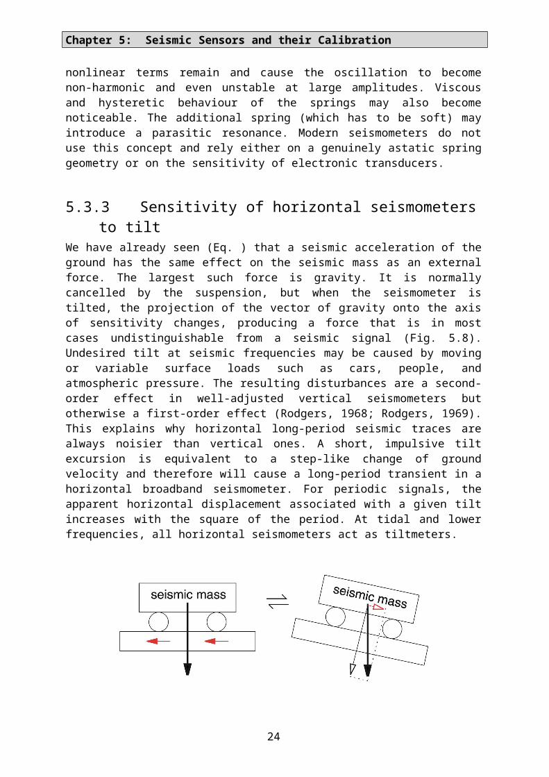
5.3.3 Sensitivity of horizontal seismometers to tiltWe have already seen (Eq. ) that a seismic acceleration of the ground has the same effect on the seismic mass as an external force. The largest such force is gravity. It is normally can-celled by the suspension, but when the seismometer is tilted, the projection of the vector of gravity onto the axis of sensitivity changes, producing a force that is in most cases undistin-guishable from a seismic signal (Fig. 5.8). Undesired tilt at seismic frequencies may be caused by moving or variable surface loads such as cars, people, and atmospheric pressure. The resulting disturbances are a second-order effect in well-adjusted vertical seismometers but otherwise a first-order effect (Rodgers, 1968; Rodgers, 1969). This explains why horizon-tal long-period seismic traces are always noisier than vertical ones. A short, impulsive tilt ex-cursion is equivalent to a step-like change of ground velocity and therefore will cause a long-period transient in a horizontal broadband seismometer. For periodic signals, the apparent horizontal displacement associated with a given tilt increases with the square of the period. At tidal and lower frequencies, all horizontal seismometers act as tiltmeters.
16
5.2 Basic theory
Fig. 5.8 The relative motion of the seismic mass is the same when the ground is acceler-ated to the left as when it is tilted to the right.
Fig. 5.9 illustrates the effect of barometrically induced ground tilt. Let us assume that the ground is vertically deformed by as little 1 m over a distance of 3 km, and that this defor-mation oscillates with a period of 10 minutes. A simple calculation then shows that seis-mometers A and C see a vertical acceleration of 10-10 m/s² while B sees a horizontal accel-eration of 10-8 m/s2. The horizontal noise is thus 100 times larger than the vertical one. In absolute terms, even the vertical acceleration is by a factor of four above the minimum ground noise in one octave as specified by the USGS Low Noise Model (5.5.1)
Fig. 5.9 Ground tilt caused by the atmospheric pressure is the main source of very-long-period noise on horizontal seismographs.
5.3.4 Direct effects of barometric pressureBesides tilting the ground, the continuously fluctuating barometric pressure affects seis-mometers in at least three different ways: (1) when the seismometer is not enclosed in a her-metic housing, the mass will experience a variable buoyancy which can cause large distur-bances in vertical sensors; (2) changes of pressure also produce adiabatic changes of tempera-ture which affect the suspension (next paragraph). Both effects can be greatly reduced by making the housing airtight or installing the sensor inside an external pressure jacket; how-ever, then (3) the housing or jacket may be deformed by the pressure and these deformations may be transmitted to the seismic suspension as stress or tilt. While it is always worthwhile to protect vertical long-period seismometers from changes of the barometric pressure, it has of-ten been found that horizontal long-period seismometers are less sensitive to barometric noise when they are not hermetically sealed. This may however cause other problems such as cor-rosion; a better approach is to use a warp-free design for the housing (see 5.5.3).
- 17 -

Chapter 5: Seismic Sensors and their Calibration
5.3.5 Effects of temperatureThe equilibrium between gravity and the spring force in a vertical seismometer is disturbed when the temperature changes. Although thermally self-compensated alloys are available for springs, using such a spring does not result in a compensated seismometer. The geometry of the whole suspension changes with temperature; the seismometer must therefore be compen-sated as a whole. However, the different thermal time constants involved prevent an efficient compensation at seismic frequencies. Short-term changes of temperature, therefore, must be suppressed by the combination of thermal insulation and thermal inertia. Special caution is required when electronic components are enclosed with the mechanical sensor: these instru-ments heat themselves up when insulated and are then very sensitive to air drafts, so the insu-lation must at the same time suppress any possible air convection (5.5.3). Long-term (sea-sonal) changes of temperature do not interfere with the seismic signal (except when they cause convection in the vault) but may drive the seismic mass out of its operating range. Eq. can be used to calculate the thermal drift of a vertical seismometer when the temperature co-efficient of the spring force is formally assigned to the gravitational acceleration.
5.3.6 Sensitivity to magnetic fieldsAll seismometers with metallic springs are to some degree sensitive to magnetic fields be-cause thermally self-compensated spring materials are magnetic. This may be noticeable when seismometers are operated in industrial areas or in the vicinity of dc-powered railway lines. Magnetic interferences by trains must especially be suspected when the long-period noise follows a regular timetable. Magnetic storms have frequently been seen in seismo-grams. At a very quiet site, the natural background variations of the geomagnetic field may limit the long-period resolution of a vertical sensor when its magnetic sensitivity exceeds 0.5 m/s2 per Tesla (Forbriger 2007, Forbriger et al. 2008). It is apparently difficult for manufac-turers to avoid this level of magnetic sensitivity. Seismometers can also accidentally acquire a remanent magnetization during manufacture, transportation or installation. Magnetic shield-ing (see 5.5.4) is therefore recommended at quiet sites.
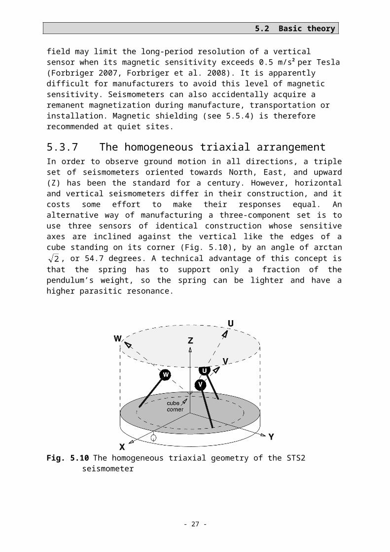
5.3.7 The homogeneous triaxial arrangementIn order to observe ground motion in all directions, a triple set of seismometers oriented to-wards North, East, and upward (Z) has been the standard for a century. However, horizontal and vertical seismometers differ in their construction, and it costs some effort to make their responses equal. An alternative way of manufacturing a three-component set is to use three sensors of identical construction whose sensitive axes are inclined against the vertical like the edges of a cube standing on its corner (Fig. 5.10), by an angle of arctan , or 54.7 degrees. A technical advantage of this concept is that the spring has to support only a fraction of the pen-dulum’s weight, so the spring can be lighter and have a higher parasitic resonance.
18
5.2 Basic theory
Fig. 5.10 The homogeneous triaxial geometry of the STS2 seismometer
The homogeneous-triaxial geometry was, with different intentions, introduced by Gal´perin (1955, 1977), Knothe (1963), and Melton and Kirkpatrick (1970), and is presently used in the Streckeisen STS2 and Nanometrics Trillium broadband seismometers. Since most seismolo-gists want finally to see the conventional E, N and Z components of motion, the oblique com-ponents U, V, W of the STS2 are electrically recombined according to
The X-axis of the STS2 seismometer is normally oriented towards East; the Y-axis then points north. Noise originating in one of the sensors of a triaxial seismometer will appear on all three outputs (except for Y being independent of U). Its origin can be traced by transform-ing the X, Y and Z signals back to U, V and W with the inverse (transposed) matrix (pro -grams TRIAX and RECTAX, see section 5.8). Disturbances affecting only the horizontal out-puts are unlikely to originate in the seismometer and are in most cases due to ground tilt. Dis-turbances of the vertical output only may be related to temperature, barometric pressure, or electrical problems common to all three sensors, such as an unstable supply voltage or vari-able internal power dissipation.
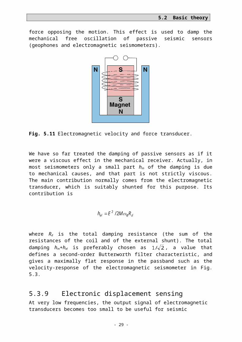
5.3.8 Electromagnetic velocity sensing and dampingThe simplest transducer both for sensing motions and for exerting forces is an electromag-netic (electrodynamic) device where a coil moves in the field of a permanent magnet, as in a loudspeaker (Fig. 5.11). Motion induces a voltage in the coil; current flowing in the coil pro-duces a force. From the conservation of energy it follows that the responsivity of the coil-magnet system as a force transducer, in Newtons per Ampere, and its responsivity as a veloc-ity transducer, in Volts per meter per second, are identical. The units are in fact the same (re-member that 1Nm = 1Joule = 1VAs). When such a velocity transducer is loaded with a resis-tor, permitting a current to flow, then according to Lenz's law it generates a force opposing the motion. This effect is used to damp the mechanical free oscillation of passive seismic sen-sors (geophones and electromagnetic seismometers).
- 19 -

Chapter 5: Seismic Sensors and their Calibration
Fig. 5.11 Electromagnetic velocity and force transducer.
We have so far treated the damping of passive sensors as if it were a viscous effect in the me-chanical receiver. Actually, in most seismometers only a small part hm of the damping is due to mechanical causes, and that part is not strictly viscous. The main contribution normally comes from the electromagnetic transducer, which is suitably shunted for this purpose. Its contribution is
where Rd is the total damping resistance (the sum of the resistances of the coil and of the ex-ternal shunt). The total damping hm+hel is preferably chosen as , a value that defines a second-order Butterworth filter characteristic, and gives a maximally flat response in the passband such as the velocity-response of the electromagnetic seismometer in Fig. 5.3.
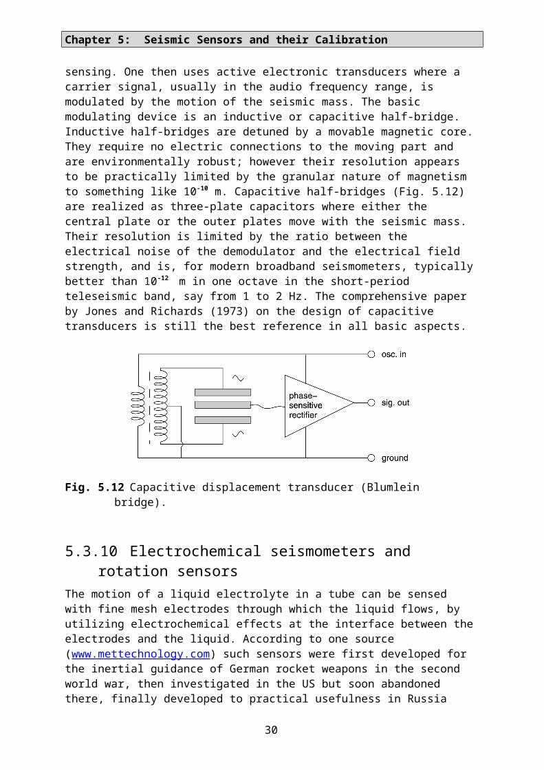
5.3.9 Electronic displacement sensingAt very low frequencies, the output signal of electromagnetic transducers becomes too small to be useful for seismic sensing. One then uses active electronic transducers where a carrier signal, usually in the audio frequency range, is modulated by the motion of the seismic mass. The basic modulating device is an inductive or capacitive half-bridge. Inductive half-bridges are detuned by a movable magnetic core. They require no electric connections to the moving part and are environmentally robust; however their resolution appears to be practically lim-ited by the granular nature of magnetism to something like 10-10 m. Capacitive half-bridges (Fig. 5.12) are realized as three-plate capacitors where either the central plate or the outer plates move with the seismic mass. Their resolution is limited by the ratio between the elec-trical noise of the demodulator and the electrical field strength, and is, for modern broadband seismometers, typically better than 10-12 m in one octave in the short-period teleseismic band, say from 1 to 2 Hz. The comprehensive paper by Jones and Richards (1973) on the design of capacitive transducers is still the best reference in all basic aspects.
20
5.2 Basic theory
Fig. 5.12 Capacitive displacement transducer (Blumlein bridge).
5.3.10 Electrochemical seismometers and rotation sensorsThe motion of a liquid electrolyte in a tube can be sensed with fine mesh electrodes through which the liquid flows, by utilizing electrochemical effects at the interface between the elec-trodes and the liquid. According to one source (www.mettechnology.com) such sensors were first developed for the inertial guidance of German rocket weapons in the second world war, then investigated in the US but soon abandoned there, finally developed to practical useful-ness in Russia based on theoretical work by V. A. Kozlov and V. Agafonof. The transducers were named Solions (from solution and ion) in the US and Molecular-Electronic (MET) by Russian authors.
In a partly filled circular tube or in a linear tube closed by elastic membranes, the liquid acts as a seismic mass, resulting in mechanically simple and very robust seismic sensors. Their transfer function is however not so simple because hydrodynamic and diffusive processes are involved. A description by poles and zeros as for pendulum-type sensors is mathematically inadequate although it can serve as an approximation. MET seismometers have some practi-cal advantages: they are small and rugged, have a low power consumption, and don’t need mass locking, mass centering or leveling. This makes them especially useful for ocean-bot-tom seismographs (see Chapter 7, section 7.5). They cannot, however, compete with observa-tory-grade pendulum instruments in other respects: resolution, precision, linearity. Force feedback is difficult to combine with the MET principle.
The MET principle is also used in rotational sensors where a circular tube is completely filled with the electrolyte. In this application they appear to be superior to mechanical devices; their symmetric design makes them virtually insensitive to linear acceleration (see IS 5.3). Rota-tional components of ground motion have been observed with MET sensors in the near-field of seismic sources, and with costly laser-gyroscopic devices at teleseismic distances from large earthquakes (see IS 2.2).
5.4 Force-balance accelerometers and seismometers
5.4.1 The force-balance principleIn a conventional passive seismometer, the inertia of the mass makes it move against the frame when the frame is accelerated, and the relative displacement or velocity of the mass is then converted into an electric signal. This principle of measurement is now used for short-period seismometers only. Broadband seismometers are built according to the force-balance principle. The inertial force is compensated (or 'balanced') with an electrically generated
- 21 -
Chapter 5: Seismic Sensors and their Calibration
force so that the seismic mass follows the motion of the frame; of course some small relative motion must remain because otherwise the inertial force could not be observed. The feedback force is generated with an electromagnetic force transducer or ‘forcer’ (Fig. 5.11). The elec-tronic circuit (Fig. 5.13) is a servo loop, like in an analog chart recorder, and adjusts the feed-back force so that the mass follows the motion of the frame.
Fig. 5.13 Feedback circuit of a force-balance accelerometer (FBA).
The servo loop is most effective when it contains an integrator, in which case the offset of the mass is exactly nulled in the time average. (In a chart recorder, the difference between the in-put signal and a voltage indicating the pen position is nulled). Due to unavoidable delays in the feedback loop, force-balance systems have a limited bandwidth; however, at frequencies where they are effective, they generate a feedback force that is proportional to ground accel-eration. When the force is proportional to the current in the transducer, then the current, the voltage across the feedback resistor R, and the output voltage are all proportional to ground acceleration. Thus we have converted the acceleration into an electric signal without depend-ing on the precision of a mechanical suspension.
The response of a force-balance system is approximately inverse to the gain of the feedback path. It can be easily modified by giving the feedback path a frequency-dependent gain. For example, if we make the capacitor C large so that it determines the feedback current, then the gain of the feedback path increases linearly with frequency and we have a system whose re-sponsivity to acceleration is inverse to frequency and thus flat to velocity over a certain pass-band. We will look more closely at this option in section 5.4.3.
5.4.2 Force-balance accelerometersFig. 5.13 without the capacitor C represents the circuit of a force-balance accelerometer (FBA), a device that is widely used for earthquake strong-motion recording, for measuring tilt, and for inertial navigation. By equating the inertial and the electromagnetic force, it is easily seen that the responsivity (the output voltage per ground acceleration) is
where M is the seismic mass, R the total resistance of the feedback path, and E the responsiv-ity of the forcer (in N/A). The conversion is determined by three passive components of which the mass is error-free by definition (it defines the inertial reference), the resistor is a nearly ideal component, and the force transducer can be very precise because the motion is
22
5.2 Basic theory
small. Some accelerometers do not have a built-in feedback resistor; the user can insert a re-sistor of his own choice and thus select the gain. The responsivity in terms of current per ac-celeration is simply .
FBAs work down to zero frequency but the servo loop becomes ineffective at some upper corner frequency f0 (usually a few hundred to a few thousand Hz), above which the arrange-ment acts like an ordinary inertial displacement sensor. The feedback loop behaves like an additional stiff spring; the response of the FBA sensor corresponds to that of a mechanical pendulum with the eigenfrequency f0, as is schematically represented in the left panels of Fig.5.3.
5.4.3 Velocity broadband seismometersFor broadband seismic recording with high sensitivity, an output signal proportional to ground acceleration is unfavorable. At high frequencies, sensitive accelerometers are easily saturated by traffic noise or impulsive disturbances. At low frequencies, a system with a re-sponse flat to acceleration generates a permanent voltage at the output as soon as the suspen-sion is not completely balanced. The system might then be saturated by the offset voltage re-sulting from thermal drift or tilt. What we need is a band-pass response in terms of accelera-tion, or equivalently a high-pass response in terms of ground velocity, like that of a normal electromagnetic seismometer (geophone, right panels in Fig. 5.3) but with a lower corner fre-quency.
The desired velocity broadband (VBB) response is obtained from the FBA circuit by adding paths for differential feedback and integral feedback (Fig. 5.14). A large capacitor C is cho-sen so that the differential feedback dominates throughout the desired passband. While the feedback current is still proportional to ground acceleration as before, the voltage across the capacitor C is a time integral of the current, and thus proportional to ground velocity. This voltage serves as the output signal. The output voltage per ground velocity, i.e. the apparent generator constant Eapp of the feedback seismometer, is
.
Again the response is essentially determined by three passive components. Although a capac-itor with a solid dielectric is not quite as ideal a component as a good resistor, the response is still linear and very stable.
Fig. 5.14 Feedback circuit of a VBB (velocity-broadband) seismometer. As in Figure 5.13, the seismic mass is the summing point of the inertial force and the negative feed-back force.
- 23 -
Chapter 5: Seismic Sensors and their Calibration
The output signal of the second integrator is normally accessible at the ,,mass position" out-put. It does not indicate the actual position of the mass but indicates where the mass would go if the feedback were switched off. ”Centering" the mass of a feedback seismometer has the effect of discharging the integrator so that its full operating range is available for the seismic signal. The mass-position output is not normally used for seismic recording but is useful as a state-of-health diagnostic, and is used in some calibration procedures.
The relative strength of the integral feedback increases at lower frequencies while that of the differential feedback decreases. These two components of the feedback force are of opposite phase (- /2 and /2 relative to the output signal, respectively). At a certain low frequency the two contributions are of equal strength and cancel each other. This is the lower corner fre-quency of the closed-loop system. Since the closed-loop response is inverse to that of the feedback path, one would expect to see a resonance in the closed-loop response at this fre-quency. However, the proportional feedback remains and damps the resonance; the resistor R acts as a damping resistor. At lower frequencies, the integral feedback dominates over the differential feedback, and the closed-loop response to ground velocity decreases with the square of the frequency. As a result, the feedback system behaves like a conventional electro-magnetic seismometer and can be described by the usual three parameters: free period, damp-ing, and generator constant. In fact, electronic broadband seismometers, even if their actual electronic circuit is more complicated than presented here, follow the simple theoretical re-sponse of electromagnetic seismometers more closely than those ever did.
As far as the response is concerned, a force-balance circuit as described here may be seen as a means to convert a moderately stable short- to medium- period suspension into a stable electronic long-period or very-long-period seismometer. The corner period can be increased by a large factor, for example 24-fold (from 5 to 120 sec) in the STS2 seismometer, 200-fold (from 0.6 to 120 sec) in CMG3 or Trillium 120 seismometers, and 600-fold in the Trillium 240. But this factor alone says little about the performance of the system. Feedback does not reduce the instrumental noise. According to Eq. , short-period suspensions must be combined with extremely sensitive displacement transducers for a satisfactory sensitivity at long peri-ods.
At some high frequency, the loop gain falls below unity. This is the upper corner frequency of the feedback system, which marks the transition from a response flat to velocity to one flat to displacement. A well-defined and nearly ideal behavior of the seismometer, like at the lower corner frequency, should not be expected here because the feedback becomes ineffec-tive and because most suspensions have parasitic resonances above the electrical corner fre-quency (otherwise they could have been designed for a larger bandwidth). The detailed re-sponse at the high-frequency corner, however, rarely matters since the upper corner fre-quency is usually outside the passband of the recorder. Its effect on the transfer function in most cases can be modeled as a small, constant delay (a few milliseconds) over the whole VBB passband.
5.4.4 Other methods of bandwidth extensionThe force-balance principle permits the construction of high-performance, broadband seismic sensors but is not easily applicable to geophone-type sensors because fitting a displacement transducer to these is difficult. Sometimes it is desirable to broaden the response of an exist-ing geophone without a mechanical redesign.
24

5.2 Basic theory
The simplest solution is to send the output signal of the geophone through a filter that re-moves its original response (this is called an inverse filtration) and replaces it by some other desired response, preferably that of a geophone with a lower eigenfrequency. The analog, electronic version of this process would only be used in connection with direct visible record-ing; for all other purposes, one would implement the filtration digitally as part of the data processing.
Alternatively, the bandwidth of a geophone may be enlarged by strong damping. This does not enhance the gain outside the passband but rather reduces it at and around the eigenfre-quency; nevertheless, after appropriate amplification, the net effect is an extension of the bandwidth towards longer periods. Strong damping is obtained by connecting the coil to a preamplifier with a negative input impedance. The total damping resistance, which is other-wise always larger than the resistance of the coil (Eq. ), can then be made arbitrarily small. The response of the over-damped geophone is flat to acceleration around its free period. It can be made flat to velocity by an approximate (band-limited) integration. This technique is used in the Lennartz Le-1d and Le-3d seismometers (DS 5.1) whose electronic corner period can be up to 40 times larger than the mechanical one. Although these are not strictly force-balance sensors, they take advantage of the fact that active damping (which is a form of nega-tive feedback) greatly reduces the relative motion of the mass.
5.5 Seismic noise, site selection and installationElectronic seismographs can be designed for any desired magnification of the ground motion. A practical limit, however, is imposed by the presence of undesired signals, which must not be magnified so strongly as to obscure the record. Such signals are usually referred to as noise and may be of seismic, instrumental, or environmental origin. Seismic noise is treated in Chapter 4; see also exercise EX_4.1. Instrumental self-noise may have mechanical and electronic sources and will be discussed in the next section. Here we focus on those general aspects of site selection and of seismometer installation aimed at the reduction of environ-mental noise. For technical details on site selection as well as vault, tunnel and borehole in-stallations see Chapter 7.
Fig. 5.15 The USGS New Low Noise Model (NLNM), here expressed as rms amplitude of ground acceleration in a constant relative bandwidth of one-sixth decade.
- 25 -
Chapter 5: Seismic Sensors and their Calibration
5.5.1 The USGS low-noise modelThe USGS low-noise model (Peterson 1993, our Fig. 5.15) is a graphical and numerical rep-resentation of the lowest vertical seismic noise levels observed worldwide, and is extremely useful as a reference for the quality of a site or of an instrument. A recent compilation of min-imum noise levels by Berger at al. (2004) has essentially confirmed the validity of the NLNM below 5 Hz; at higher frequencies the NLNM appears to be somewhat too low. Origin and properties of seismic noise are discussed in Chapter 4.
5.5.2 Site selection and vault designSite selection for a permanent station is always a compromise between two conflicting re-quirements: infrastructure and low seismic noise. The noise level depends on the geological situation and on the proximity of sources, some of which are usually associated with the in-frastructure. A seismograph installed on solid basement rock can be expected to be fairly in-sensitive to local disturbances while one sitting on a thick layer of soft sediments will be noisy even in the absence of identifiable sources. As a rule, the distance from potential sources of noise, such as roads, industry, and inhabited houses, should be very much larger than the thickness of the sediment layer. Broadband seismographs can be successfully oper-ated in major cities when the geology is favorable; in unfavorable situations, such as in sedi-mentary basins, only deep mines and boreholes may offer acceptable noise levels (see 4.3.2, 7.4.3 and 7.4.5).
By definition of the Low Noise Model, most sites have a noise level above the NLNM, some-times by a large factor. This factor, however, is not uniform over time or over the seismic fre-quency band. At short periods (< 2 s), a noise level within a factor of 10 of the NLNM may be considered very good in most areas. Short-period noise at most sites is predominantly man-made, lower during nighttime, and somewhat larger in the horizontal components than in the vertical. At intermediate periods (2 to 20 s), marine microseisms dominate. They have similar amplitudes in the horizontal and vertical components and have large seasonal varia-tions. In winter they may be 50 dB above the NLNM. At longer periods, vertical ground noise is often within 10 or 20 dB of the NLNM even at otherwise noisy stations. Horizontal long-period noise may nevertheless be horrible at the same station due to tilt-gravity coupling (5.3.3). It may be larger than vertical noise by a factor of up to 300, the factor increasing with period. Therefore, a site can be considered as favorable when the horizontal noise at 100 to 300 sec is within 20 dB (i.e., a factor of 10 in amplitude) above the vertical noise. Tilt may be caused by traffic, wind, or local fluctuations of the barometric pressure. Large tilt noise is sometimes observed on concrete floors when an unventilated cavity exists underneath; the floor then acts like a membrane. Such noise can be identified by its linear polarization and its correlation with the barometric pressure. Even on an apparently solid foundation, the long-period noise often correlates with the barometric pressure (Beauduin et al., 1996). If the situa-tion cannot be remedied otherwise, the barometric pressure should be recorded with the seis-mic signal and used for a correction. An example of barometric noise is shown in Fig. 2.21 of the NMSOP. For very-broadband seismographic stations, barometric recording is generally recommended.
Besides ground noise, environmental conditions must be considered. An aggressive atmos-phere may cause corrosion, wind and short-term variations of temperature may induce noise, and seasonal variations of temperature may exceed the manufacturer’s specifications for unattended operation. Seismometers must be protected against these conditions, sometimes by hermetic containers as described in the next subsection. Suggestions for vault design have
26
5.2 Basic theory
been given by Uhrhammer and Karavas (1997) and Trnkoczy (1998) and more recently by the PASSCAL Instrument Center (2009a). Since it is difficult to prevent water from accumu-lating in vaults, installation of a drainage or a sump pump should be considered (Passcal In-strument Center 2009b).
5.5.3 Seismometer installationWe describe briefly the installation of a portable broadband seismometer inside a building, vault, or cave. First, the orientation of the sensor is marked on the floor. This is best done with a geodetic gyroscope, but a magnetic compass will do in most cases. The magnetic dec-lination must be taken into account. Since a compass may be deflected inside a building, the direction should be taken outside and transferred to the site of installation. Spirit levels com-bined with a laser, and especially laser cross levels, are most convenient tools for orienting seismometers, and are available at low cost from do-it-yourself stores. When the magnetic declination is unknown or unpredictable (such as at high latitudes or in volcanic areas), the orientation can be determined with a sun compass.
Fig. 5.16 The STS2 seismometer of the GRSN inside its shields.
To isolate the seismometer from stray currents, small glass or Plexiglas plates should be ce-mented to the ground under its feet. Then the seismometer is installed, tested, and wrapped with a layer of soft, thermally insulating material such as fiber wool or a fleece blanket. It is essential that this inner heat shield is so soft that it cannot transport substantial forces to the sensor. An additional heat-reflecting blanket (commonly sold as “rescue blanket”) protects the sensor from thermal radiation and air drafts. It should also cover the floor around the seis-mometer. The use of Styrofoam seeds is not recommended; they have been observed to cause mechanical noise. Stiff shields such as Styrofoam boxes provide additional protection but must not touch the sensor. The self-heating of electronic seismometers can induce convection in any open space inside the insulation; it is therefore important that the insulation leaves no gap around the seismometer, or at most a gap that is only a few millimeters wide.
For a permanent installation under unfavourable environmental conditions, the seismometer should be enclosed in a hermetic container. A problem with such containers (as with all seis-mometer housings) is, however, that they cause tilt noise when they are deformed by the ba-
- 27 -
Chapter 5: Seismic Sensors and their Calibration
rometric pressure. Essentially three precautions are possible: (1) either the base-plate is care-fully cemented to the floor, or (2) it is made so massive that its deformation is negligible, or (3) a “warp-free” design is used, as described by Holcomb and Hutt (1992) for the STS1 seis-mometer. Some fresh desiccant (Silica gel) should be placed inside the container, even into the vacuum bell of STS1 seismometers. Cable connectors corrode easily in a humid environ-ment. All external connectors and auxiliary electronic equipment should therefore be protec-ted with closed (as far as possible) plastic bags and desiccant. Figure 5.16 illustrates the shielding of the STS2 seismometers in the German Regional Seismic Network (GRSN).
5.5.4 Magnetic shieldingMagnetic shields can be manufactured from Permalloy (Mu-Metal) but they are expensive and of limited efficiency. An active compensation may be preferable. Such a device might consist of a three-component fluxgate magnetometer that senses the field near the seismome-ter, an electronic driver circuit in which the signals are integrated with a short time constant (a few milliseconds) and amplified, and a three-component set of Helmholtz coils through which the output current is sent in order to compensate changes of the magnetic field. The permanent geomagnetic field should not be compensated; the resulting offsets of the fluxgate outputs can be compensated electrically before the integration, or with permanent magnets mounted rigidly near the fluxgate.
5.5.5 Instrumental self-noiseAll modern seismographs use semiconductor amplifiers, which like other active (power-dissi-pating) electronic components produce continuous electronic noise whose origin is manifold but ultimately related to the quantization of the electric charge. Electromagnetic transducers, such as those used in geophones, also produce thermal electronic noise (resistor noise, John-son noise). The contributions from semiconductor noise and resistor noise are often compara-ble, and together limit the sensitivity of the system. Another source of continuous noise, the Brownian (thermal) motion of the seismic mass, may be noticeable when the mass is very small (less than a few grams). Presently manufactured observatory-grade seismometers have sufficient mass to make the Brownian noise negligible against noise from other sources and we will therefore not discuss it here. Seismographs may also suffer from transient distur-bances originating in slightly defective semiconductors or in stressed mechanical parts of the seismometer. The present section is mainly concerned with identifying and measuring instru-mental noise.
5.5.6 Self-noise of electromagnetic seismographsElectromagnetic seismometers and geophones are passive sensors whose self-noise is of purely thermal origin and does not increase at low frequencies as it does in active (power-dis-sipating) devices. Their output signal is however comparatively small, so a low-noise pream-plifier (Fig. 5.17) must be inserted between the geophone and the recorder. We will call this combination an electromagnetic seismograph or EMS. Unfortunately the preamplifier noise does increase at low frequencies and limits the overall sensitivity. EMSs are now rarely used for long-period or broadband recording because of the superior performance of feedback in-struments.
The sensitivity of an EMS is normally limited by amplifier noise. However, this noise does not depend on the amplifier alone but also on the impedance of the electromagnetic trans-
28
5.2 Basic theory
ducer coil, which can be chosen within wide limits. Up to a certain impedance the amplifier noise voltage is nearly constant, but then it increases linearly with the impedance, due to a noise current flowing out of the amplifier input. On the other hand, the signal voltage in-creases with the square root of the coil impedance. The best signal-to-noise ratio is therefore obtained with an optimum source impedance defined by the corner between voltage and cur-rent noise in the graph of total noise vs. source impedance, and is different for each type of amplifier and also depends on frequency. Vice versa, when the transducer is given, the ampli-fier must be selected for low noise at the relevant impedance and frequency.
Fig. 5.17 Two alternative circuits for an EMS preamplifier with a low-noise op-amp. The non-inverting circuit is generally preferable when the damping resistor Rl is much larger than the coil resistance and the inverting circuit when it is comparable or smaller. However, the relative performance also depends on the noise specifica-tions of the op-amp. The gain is adjusted with Rg.
The electronic noise of an EMS can be predicted when the technical data of the sensor and the amplifier are known. Semiconductor noise increases at low frequencies; amplifier specifi-cations must apply to seismic rather than audio frequencies. In combination with a given sen-sor, the noise can then be expressed as an equivalent seismic noise level and compared to real seismic signals or to the NLNM (Fig. 5.15). As an example, Fig. 5.18 shows the self-noise of one of the better seismometer-amplifier combinations. It resolves minimum ground noise be-tween 0.1 and 10 s period. Discussions and more examples are found in Riedesel et al. (1990) and in Rodgers (1992, 1993 and 1994). Their result is easily summarized:
Fig. 5.18 Electronic self-noise of the input stage of a short-period seismograph. The EMS is a Sensonics Mk3 with two 8 kOhm coils in series and tuned to a free period of 1.5 s. The amplifier is the LT1012 op-amp. The curves a and b refer to the circuits of Fig. 5.17. NLNM is the USGS New Low Noise Model (Fig. 5.15). The ordinate gives rms noise amplitudes in dB relative to 1 m/s2 in 1/6 decade.
- 29 -
Chapter 5: Seismic Sensors and their Calibration
Most well-designed seismometer-amplifier combinations resolve minimum ground noise up to 6 or 8 s period, that is, to the microseismic peak. A few of them may make it to about 15 s; they marginally resolve the secondary microseismic peak. To resolve mini-mum ground noise up to 30 s is hopeless, as is obvious from Fig. 5.18. Ground noise falls and electronic noise rises so rapidly beyond a period of 20 s that the crossover point can not be substantially moved towards longer periods. Of course, at a reduced level of sensi-tivity, restoring long-period signals from short-period sensors may make sense, and the long-period surface waves of sufficiently large earthquakes may well be recorded with short-period electromagnetic seismometers.
Amplifier noise can be observed by locking the sensor or tilting it so that the mass is firmly at a stop, or by replacing it with a resistor that has the same resistance as the coil. If these ma-nipulations do not significantly reduce the noise, then obviously the EMS does not resolve seismic noise. However, this is only a test, not a way to precisely measure the electronic self-noise. A locked sensor or a resistor do not exactly represent the electric impedance of the un-locked sensor (see 5.6.3).
5.5.7 Self-noise of force-balance seismometersAlthough the self-noise of force-balance seismometers can theoretically be predicted from that of its components, such a prediction may be unrealistic because certain sources of noise appear only under operating conditions. Anyhow, the user can hardly test the components without destroying the instrument. The electronic circuit cannot be tested when the mass is locked. The instrumental noise can thus only be observed under operating conditions, in the presence of seismic and environmental noise.
Although seismic noise is generally a nuisance in this context, natural signals may also be useful as test signals. Marine microseisms should be visible on any sensitive seismograph whose seismometer has a free period of one second or longer. They normally are the strong-est continuous signal in a broadband trace. However, their amplitude exhibits large seasonal and geographical variations. For broadband seismographs at quiet sites, the tides of the solid Earth are a reliable and predictable test signal. They have a predominant period of slightly less than 12 hours and an amplitude in the order of 10-6 m/s2. While normally invisible in the raw data, they may be extracted by low-pass filtration with a corner frequency of 1 mHz. For this purpose it is helpful to have the data available with a sampling rate of 1 per second or less. By comparison with the predicted tides, the gain and polarity of the seismograph may be checked (e.g. Davis and Berger 2007). A seismic broadband station that records tides is likely to be up to international standards.
5.5.8 Coherency analysisFor a quantitative determination of instrumental noise, two or three instruments must be oper-ated side by side (Holcomb 1989, 1990; Sleeman et al. 2006). One can then determine the co-herency between the records and assume that coherent noise is seismic and incoherent noise is instrumental. This works well if one has a quiet site and a good reference instrument, but the method is not safe. The seismometers may respond coherently to environmental distur-bances caused by barometric pressure, temperature, the supply voltage, magnetic fields, vi-brations, or electromagnetic waves. Nonlinear behavior (intermodulation) may produce co-herent but spurious long-period signals. When no good reference instrument is available, then
30
5.2 Basic theory
different instrument types should be used in the test that are unlikely to respond in the same way to environmental disturbances.
The coherency analysis is somewhat tricky in detail when only two instruments are available. When the transfer functions of both instruments are precisely known, it is in fact theoretically possible to determine the seismic signal and the instrumental noise of each instrument sepa-rately as a function of frequency. Alternatively, one may assume that the transfer functions are not so well known but the reference instrument is noise-free; in this case the noise and the relative transfer function of the other instrument can be determined. The coherency analysis with three instruments after Sleeman et al. (2006) permits the determination of the relative transfer function and the instrumental noise of each instrument at the same time, so it requires no questionable assumptions. It may fail, however, when physically different sources of noise are present (such as seismic and magnetic noise) to which the instruments do not have a uni-form response. As with all statistical methods, very long time series or multiple observations are required for significant results. We offer the computer programs TWOCROSP and TRI-CROSP for the analysis (section 5.8).
5.5.9 Transient disturbancesMost new seismometers produce spontaneous transient disturbances, quasi miniature earth-quakes caused by stresses in the mechanical components. Although they do not necessarily originate in the spring, their waveform at the output seems to indicate a sudden and perma-nent (step-like) change in the spring force. Long-period seismic records are sometimes se-verely degraded by such disturbances. The transients often die out within months or years; if they do not, and especially when their frequency increases, corrosion must be suspected. Manufacturers try to mitigate the problem with a low-stress design and by aging the compo-nents or the finished seismometer (by extended storage, vibrations, or heating and cooling cy-cles). It is sometimes possible to release stresses and eliminate transient disturbances by hit-ting the pier around the seismometer with a hammer, a procedure that is recommended for each new installation.
5.6 Calibration
5.6.1 Electrical and mechanical calibrationThe calibration of a seismometer establishes knowledge of the relationship between its input (the ground motion) and its output (an electric signal), and is a prerequisite for a reconstruc-tion of the ground motion. Since precisely known ground motions are difficult to generate, one makes use of the equivalence between ground acceleration and an external force on the seismic mass, and calibrates seismometers with an electromagnetic force generated in a cali-bration coil. This is called an electrical or relative calibration. In the case of feedback seis-mometers an electrical calibration essentially characterizes the electronic feedback circuit but not the mechanical receiver. The absolute responsivity to ground motion can be determined from an electric calibration only if the factor of proportionality between the current in the coil and the equivalent ground acceleration is known,. Otherwise, it must be determined from a mechanical experiment in which the seismometer is actually moved. This is called a mechan-ical or absolute calibration. Since precise mechanical input signals are difficult to generate over a large bandwidth, one does not normally attempt to determine the complete transfer function in this way.
- 31 -

Chapter 5: Seismic Sensors and their Calibration
Paragraphs 5.6.2 to 5.6.7 are mainly concerned with the electrical (relative) calibration al-though some methods may also be used for the mechanical calibration on a shake table (5.6.9). Procedures for the absolute mechanical calibration that do not require a shake table are presented in 5.6.10 and 5.6.11.
5.6.2 General conditionsCalibration experiments are disturbed by seismic noise and tilt and should therefore be car-ried out in a basement room. However, the large operating range of modern seismometers permits a calibration with relatively large signal amplitudes, making background noise less of a problem than one might expect. Thermal drift is more serious because it interferes with the long-period response of broadband seismometers. For a calibration at long periods, seis-mometers must be protected from air draft and allowed sufficient time to reach thermal equi-librium. Visible and digital recording in parallel is recommended. Recorders themselves must be absolutely calibrated before they can serve to absolutely calibrate seismometers. The in-put impedance of recorders and the source impedance of sensors must be measured or looked up in the manuals so that a correction can be applied for the voltage drop in the source impedance.
5.6.3 Specific procedures for geophonesGeophones usually have no calibration coil. The calibration current must then be sent through the signal coil where it produces an ohmic voltage in addition to the output signal generated by the motion of the mass. The undesired voltage can be compensated in a bridge circuit (Willmore 1959); the bridge is zeroed with the seismic mass locked or at a stop. When the calibration current and the output voltage are digitally recorded, it is more convenient to use only a half-bridge (Fig. 5.19) and to compensate the ohmic voltage numerically. The program CALEX (section 5.8) can do this automatically. The residual (the difference between the ac-tual and the modeled response) is often dominated by nonlinear distortions (section 5.7).
Fig. 5.19 Half-bridge circuit for calibrating electromagnetic seismometers
Geophones can be absolutely calibrated without a mechanical input provided that the total moving mass M is known and its motion is linear. In an electric calibration a geophone be-haves like a resonant electric circuit. Its electrical impedance is
32
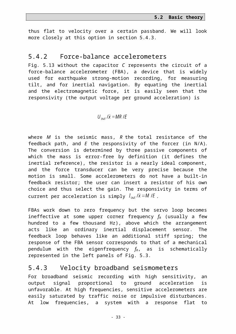
5.2 Basic theory
RC is the ohmic resistance of the coil, E is the generator constant of the electromagnetic trans-ducer as in 5.2.8. The term after the plus sign is the response of a resonant electric circuit consisting of a capacitor C=M/E2, an inductor L=E2/S, and a resistor RD=E2/2D in parallel. M, S, and D are the mechanical components of the pendulum as in 5.2.7. The analysis of the resonant response, either in time or in frequency domain, supplies all desired parameters when M is known. For an analysis in time domain, it is convenient to excite a transient re-sponse by interrupting a current through the signal coil (Willmore 1979, Rodgers et al. 1995). In this case the ohmic voltage disappears when the transient response begins. CALEX can also be used here.
Fig. 5.20 Determining the generator constant from a plot of damping versus total damping resistance Rd = Rcoil + Rload. The horizontal units are microsiemens (reciprocal Megohms).
Another approach is illustrated in Fig. 5.20. The electromagnetic part of the numerical damp-ing is inversely proportional to the total damping resistance, the factor of proportionality be-ing . The generator constant E can thus be calculated from relative calibrations with different resistive loads, independent of the method used for the relative calibration.
5.6.4 Calibration with sinewaves (obsolete)With a sinusoidal input, the output of a linear system is also sinusoidal, and the ratio of the two signal amplitudes is the absolute value of the transfer function. An experiment with sinewaves therefore permits a direct check of the transfer function, without any a-priori knowledge of its mathematical form and without waveform modeling. This is often the first step in the identification of an unknown system. A computer program would however be re-quired to derive a parametric representation of the response from the measured values. A cali-bration with arbitrary signals, as described later, is more straightforward for this purpose.
Calibration with sinewaves is time-consuming because the system must reach a steady state after each change of frequency, which can take more than 10 minutes for some broadband seismometers. The gain and phase delay can be read manually from a plotted Lissajous el-lipse as in Fig. 5.21. The accuracy of the evaluation depends on the purity of the sinewave. A better accuracy is obtained by numerical analysis of digitally recorded data. By fitting sinewaves to the signals, amplitudes and phases can be extracted for just one precisely known frequency at a time; distortions of the input signal don't matter then. If the test frequency is not digitally controlled, then it should be fitted as well. The fit should be computed for an in-
- 33 -
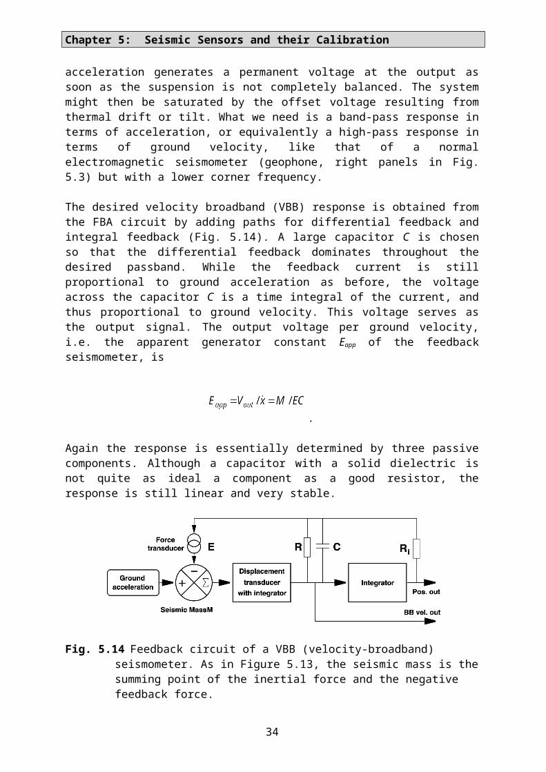
Chapter 5: Seismic Sensors and their Calibration
teger number of cycles, and offsets should be removed from the data. We offer a computer program ,,SINFIT" for this purpose (section 5.8). Although the method is now obsolete for the purpose of calibration, it is useful for investigating unmodelled details of the response such as parasitic resonances; these might be lost in a more time-efficient broadband calibra-tion. Another surviving application is the calibration of passive short-period seismometers in seismic stations where sinewaves can be remotely applied to the calibration coil but no other test signals are available. The evaluation can be done with the SINCAL program (section 5.8).
Fig. 5.21 Measuring the phase between two sine-waves with a Lissajous ellipse.
Eigenfrequency f0 and damping h of seismometers with a conventional response can be deter-mined graphically with a set of standard resonance curves on double-logarithmic paper. The measured amplitude ratios are plotted as a function of frequency f on the same type of paper and overlain with the standard curves (Fig. 5.22). The desired quantities can be read directly. The method is simple but not very accurate.
Fig. 5.22 Normalized resonance curves.
34
5.2 Basic theory
5.6.5 Step response and weight-lift test (obsolete)The simplest but only moderately accurate and now historical calibration method is to ob-serve the response of the system to a step input. The step signal can be generated by switch-ing on or off a current through the calibration coil, or by applying or removing a constant me-chanical force on the seismic mass, usually by lifting a weight. Horizontal sensors used to be absolutely calibrated with a V-shaped thread attached to the mass at one end, to a fixed point at the other end, and to the test weight at half length. The thread was then burned off for a soft release.
The step-response experiment can be used both for a relative and an absolute calibration; when applicable, it is probably the simplest method for the latter. Using a known test weight w and knowing the seismic mass M, we also know the test signal: it is a step in acceleration whose magnitude is w/M times gravity (times a geometry factor when the force is applied through a thread). In case of a rotational pendulum, a correction factor must be applied when the force does not act at the center of gravity. The method has lost its former importance be-cause the seismic mass of modern seismometers is not easily accessible, and no correction factor for rotational motion is supplied by the manufacturers.
Fig. 5.23 Normalized step responses of second-order high-pass, band-pass, and low-pass fil-ters.
In the context of relative calibration, the step-response method is still useful as a quick and intuitive test, and has the advantage that it can be visually evaluated. The CALEX method covers the step response as well. Fig. 5.23 shows the characteristic step responses of second-order high-pass, band-pass, and low-pass filters with of critical damping.
Each response is a strongly damped oscillation around its asymptotic value. With the speci-fied damping, the systems are Butterworth filters, and the amplitude decays to or 4.3% in each half cycle. The ratio of two subsequent amplitudes of opposite polarity is known as the overshoot ratio. It can be evaluated for the numerical damping h: when xi and xi+n are two (peak-to-peak) amplitudes n cycles apart, with integer or half-integer n, then
The free period can, in principle, also be determined from the impulse or step response of the damped system but should be measured preferably without electrical damping so that more oscillations can be observed. A system with the free period T0 and damping h oscillates with the period and the overshoot ratio . The manual evaluation of a step response is explained in worksheet WS_5.3.
- 35 -

Chapter 5: Seismic Sensors and their Calibration
5.6.6 Calibration with arbitrary signals In most cases, the purpose of calibration is to obtain the parameters of an analytic representa-tion of the transfer function. Its mathematical form is normally known a priori. What remains is to determine a number of discrete parameters (such as corner periods and damping con-stants) from an experiment in which the response to a known input signal is observed. One uses either a predetermined input signal that is numerically reconstructed in the analysis, or an arbitrary input signal that is recorded together with the output signal. Only a recorded sig-nal is reliably and precisely known. Recording both signals with the same recorder has the additional advantage of eliminating the transfer function of the recorder from the analysis.
Fig. 5.24 Block diagram of the CALEX procedure. Storage and retrieval of the data are omitted from the figure.
Calibration is a classical inverse problem that can be solved with standard least-squares meth-ods. The general solution is schematically depicted in Fig. 5.24. A computer algorithm (filter 1) is implemented that represents the seismometer as a filter and permits the computation of its response to an arbitrary input. An inversion scheme (3) is programmed around the filter al-gorithm in order to find best-fitting filter parameters for a given pair of input and output sig-nals. The purpose of the anti-alias filters (2) is explained below. The sensor is then excited with a test signal (4) that must have a suitable frequency content but is otherwise arbitrary. When the system is linear, parameters obtained from one test signal determine the response to any other signal.
When the transfer function has been correctly parameterized and the inversion has converged, then the residual error consists mainly of noise, drift, and nonlinear distortions. At a signal level of about half of the operating range, typical residuals are 0.02% to 0.05% rms for force- balance seismometers and 1% for passive electrodynamic sensors.
The approximation of a rational transfer function with a discrete filtering algorithm is not trivial. The program CALEX (section 5.8) uses an impulse-invariant recursive filter (Schuessler, 1981). This method formally requires that the seismometer has a negligible re-sponse at frequencies outside the Nyqvist bandwidth of the recorder, a condition that is se-verely violated by most digital seismographs; but this problem can be circumvented with an additional digital low-pass filtration (Filter 2 in Fig. 5.24) that limits the bandwidth of the simulated system. Signals from a typical calibration experiment are shown in Fig. 5.25. A sweep as a test signal permits the residual error to be visualized as a function of time or fre-quency. Since essentially only one frequency is present at a time, the time axis may as well be interpreted as a frequency axis.
36
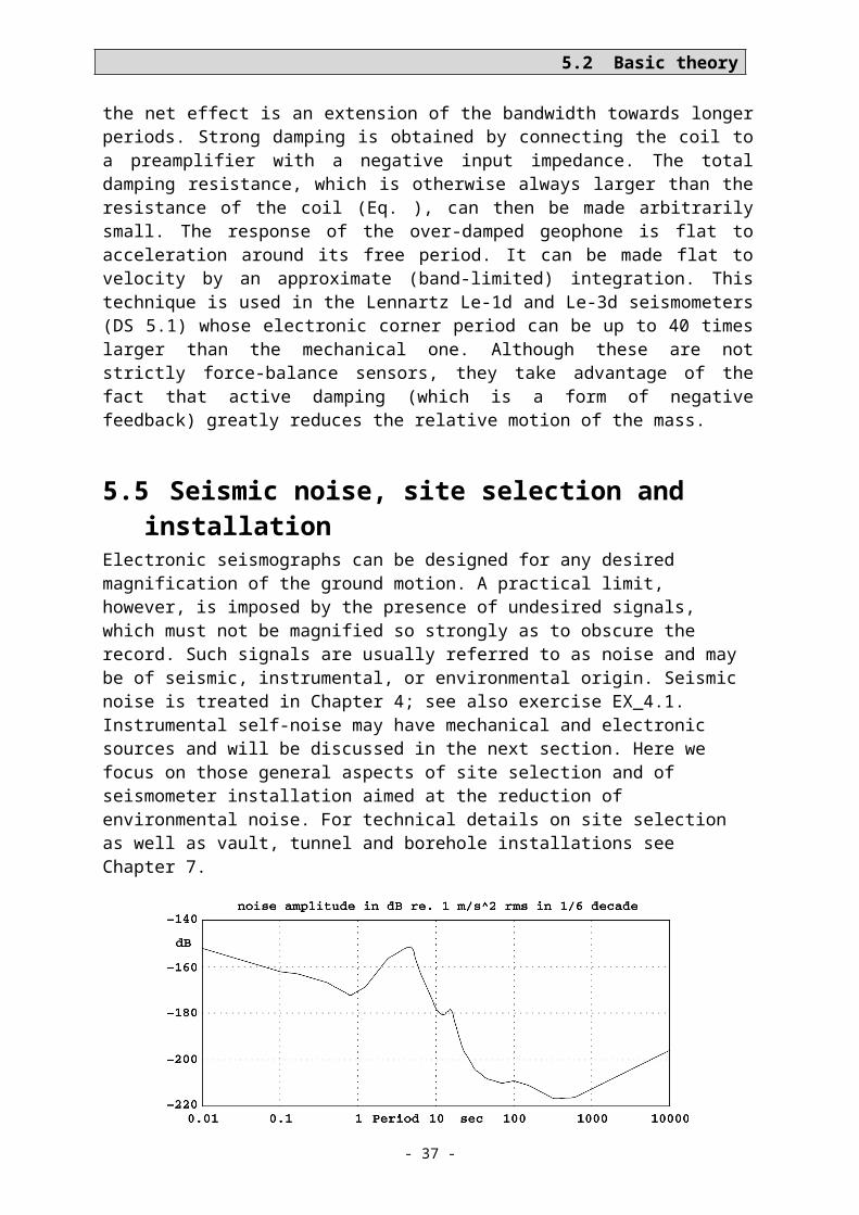
5.2 Basic theory
Fig. 5.25 Electrical calibration of an STS2 seismometer with CALEX. Traces from top to bottom: input signal (a sweep with a total duration of 10 min); output signal; syn-thetic output signal; residual. The rms residual is 0.05 % of the rms output. See also exercise EX_5.4.
With an appropriate choice of the test signal, other methods like the calibration with sine-waves, step functions, random noise or random telegraph signals, can be duplicated and com-pared to each other. An advantage of a CALEX type algorithm is that it makes no use of spe-cial properties of the test signal, such as being sinusoidal, periodic, step-like or random. Therefore, test signals can be short (a few times the free period of the seismometer) and can be generated with the most primitive means, even by hand (you may turn the dial of a sinewave generator by hand, or even produce the test signal with a battery and a switch or po-tentiometer). A breakout box or a special cable may however be required for feeding the cali-bration signal into the digital recorder.
For a quick and easy check of the transfer function, the simple method of spectral division may be sufficient. When the input signal (the stimulus) and the output signal (the response) have both been recorded, and the system was quiet at the beginning and the end of the record, then dividing the amplitude spectrum of the output signal by that of the input signal may re-sult in a reasonable approximation to the actual response, at least in a limited bandwidth. A parametric (mathematical) representation of the response, such as by poles and zeros, is how-ever more difficult to obtain in this way.
Some other routines for seismograph calibration and system identification are contained in the PREPROC software package (Plešinger et al., 1996).
5.6.7 Specific procedures for triaxial seismometersIn homogeneous-triaxial seismometers such as the Streckeisen STS2 and the Nanometrics Trillium models, transfer functions in a strict sense can only be attributed to the individual U, V, W sensors, not to the X, Y, Z outputs. Formally, the response of a triaxial seismometer to
- 37 -
Chapter 5: Seismic Sensors and their Calibration
arbitrary ground motions is described by a nearly diagonal 3 x 3 matrix of transfer functions relating the X, Y, Z output signals to the X, Y, Z ground motions. This is also true for con -ventional three-component sets if they are not perfectly aligned; only the composition of the matrix is slightly different.
However, if the U, V, W sensors are reasonably well matched, then we need not care about a matrix of transfer functions. The X, Y, Z channels can then each be described by a single transfer function that is a weighted averages of those of the U, V, W sensors:
This formula applies to transfer functions or parameters but not to signals; the matrix ele-ments in are the squares of those in . For any real instrument they will differ slightly from their nominal values but this is negligible in the present context.
The X, Y, Z outputs can thus be calibrated as if they represented single-component sensors. In order to simulate a ground acceleration in one of the X, Y, or Z directions, simultaneous currents must be sent through the U, V, W calibration coils so that an output signal appears only at one of the X, Y, Z outputs. For the Z component this requires equal currents through the U, V, W coils. For the X or Y direction, the three currents must however have different magnitudes and polarities, which requires a slightly more complicated test arrangement. This inconvenience is circumvented by a procedure introduced by Peter Davis (UCSD): calibrate the vertical output with equal currents into the U, V, W coils but record the X and Y output signals as well. Unless all transfer functions happen to be identical, small residual signals will appear at the X and Y outputs. They contain information on the X and Y transfer functions. Use the inverse (transposed) of the signal transformation matrix to reconstruct the U, V, W signals, analyse these for their transfer functions, and recombine the results according to . A computer program TRICAL, essentially a combination of TRIAX and CALEX, is available for this procedure (see 5.8). The experiment normally requires four digitizer channels; if only three are available, one must use a predetermined stimulus such as a pseudo-random tele-graph signal that can be numerically duplicated.
5.6.8 Calibration and orientation against a reference sensorUsing ground noise or other seismic signals, an unknown sensor can be calibrated against a known one by operating the two sensors side by side (Pavlis and Vernon, 1994). The method is limited to a frequency band where suitable seismic signals occur well above the instrumen-tal noise level and are spatially coherent between the two instruments. The instruments must be close to each other on the same pier. The frequency response and the gain of the unknown instrument can be determined at the same time. We offer a program INVERSEIF (section 5.8) for the analysis. If the frequency response of both sensors is already known or can be measured electrically, then it will suffice to deconvolve both records to a common response and compare the signal amplitudes in a frequency band where the waveforms are identical.
In a similar way, the orientation of a three-component borehole seismometer may be deter-mined by comparison with a reference instrument at the surface. The mathematical problem can be formulated as follows: for each component yi of the borehole seismometer find a set of three directional coefficients ai1, ai2, ai3 so that the output signal yi is best represented by yi = ai1 x1 + ai2 x2 + ai3 x3 in a least-squares sense, where x1, x2, x3 are the output signals of the
38
5.2 Basic theory
three components of the reference sensor. Almost any seismic signal that is recorded with a good signal-to-noise ratio can be used as a test signal. Instrumental responses must be nor-malized (deconvolved to a common frequency response) and an additional band-pass filtra-tion is recommended. The 3*3 matrix A = (aik) contains information both on the orientation and on the orthogonality of the borehole sensor (assuming proper orientation and orthogonal-ity of the reference sensor). The instruments can also be interchanged in the formulation of the problem; one then obtains the inverse matrix that is needed to correct the borehole sig-nals. We offer the LINCOMB3 software (section 5.8) for calculating the aik coefficients. Commercial packages for linear algebra like MATLAB also offer convenient solutions.
5.6.9 Calibration on a shake tableUsing a shake table is the most direct way of obtaining an absolute calibration. In practice, however, precision is usually poor outside a frequency band roughly from 0.5 to 5 Hz. At higher frequencies, a shake table loaded with a broadband seismometer may develop parasitic resonances, and inertial forces may cause uncontrolled motions. At low frequencies, the max-imum displacement and thus the signal-to-noise ratio may be insufficient, and the motion may be non-uniform due to friction or roughness in the bearings. Still worse, most shake ta-bles do not produce a purely translational motion but also some tilt. Gravity is then coupled into the seismic signal. Its relative contribution increases with the square of the signal period and causes an intolerable error in the horizontal components at long periods. One might think that a tilt of 10 rad per mm of linear motion should not matter; however, at periods longer than 20 s, such tilt will cause a larger output signal than the linear motion. At a period of 1 s, the effect would be negligible. Long-period measurements on a horizontal shake table, if pos-sible at all, require extreme care.
Electromagnetic shake tables may also have large magnetic stray fields. These can be picked up by electromagnetic transducers or electronic circuits in the sensor so strongly that no cali-bration is possible at any frequency.
Although most calibration methods mentioned in the previous section are applicable on a shake table, the preferred method is to record both the motion of the table (as measured with a displacement transducer) and the output signal of the seismometer, and to analyze these sig-nals by linear modeling with CALEX (section 5.8) or equivalent software. Depending on the definition of active and passive parameters, one might determine only the absolute gain (re-sponsivity, generator constant) or any number of additional parameters of the frequency re-sponse. CALEX permits the automatic elimination of tilt effects, under the assumption that the tilt is proportional to the displacement.
5.6.10 Calibration by stepwise motionThe movable tables of machine tools like lathes and milling machines, and of mechanical bal-ances, can replace a shake table for the absolute calibration of seismometers. Also, a portable “step table” for seismometer calibration is now commercially available. The idea is to place the seismometer on the table, let it come to equilibrium, then move the table by a known amount and let it rest again. The apparent motion of the frame can be calculated by inverse filtration of the output signal and compared with the known mechanical displacement. Since the calculation involves triple integrations, offset and drift must be carefully removed from the seismic trace. The main contribution to drift in the apparent horizontal velocity comes from tilt associated with the motion of the table. With the method subsequently described, it is possible to separate the contributions of displacement and tilt from each other so that the
- 39 -
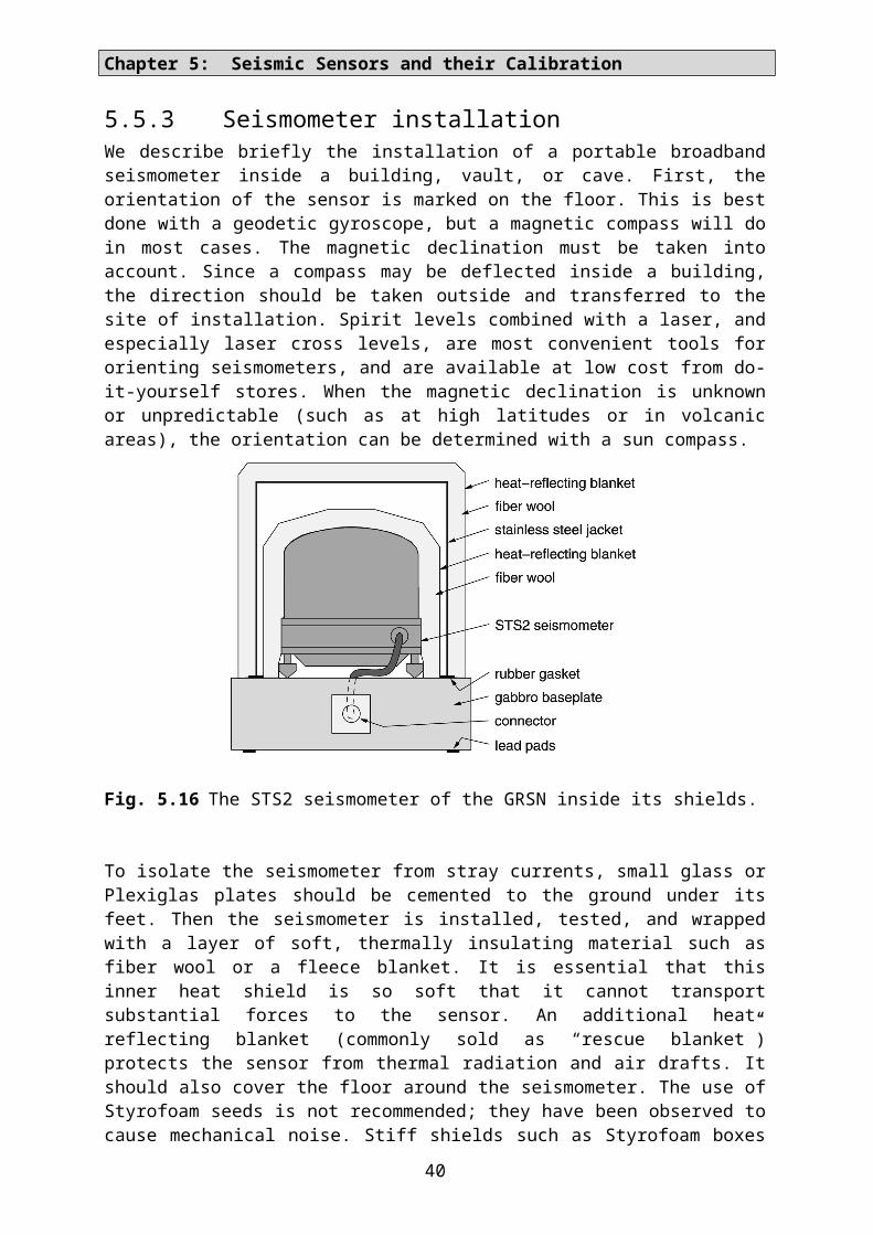
Chapter 5: Seismic Sensors and their Calibration
displacement can be reconstructed with good accuracy. This method of calibration is most convenient because it uses only normal workshop equipment. The inherent precision of ma-chine tools and the use of relatively large motions eliminate the difficulty of measuring small mechanical displacements. A FORTRAN program DISPCAL is available for the evaluation (section 5.8).
The precision of the method depends on avoiding two main sources of error:
1 - Restoring ground displacement from the seismic signal (a process of inverse filtration) is uncritical for broadband seismometers but requires a precise knowledge of the transfer func-tion for short-period seismometers. Instruments with unstable parameters (such as electro-magnetic seismometers) must be electrically calibrated while installed on the test table. How-ever, once the response is known, restoring the absolute ground displacement is no problem even for a geophone with a free period of 0.1 s.
2 - The effect of tilt can only be removed from the displacement signal when the motion is sudden and short. The tilt is unknown during the motion, and since it is equivalent to an ac-celeration, it produces unknown offsets and trends in the displacement trace that cannot be distinguished from a true displacement. The magnitude of this error signal can however be estimated from the apparent velocity observed when the true motion has ended. In contrast, static tilt before and after the motion produces linear trends in the velocity, which are easily removed.
The computational evaluation consists in the following major steps:1) the trace is de-convolved with the velocity transfer function of the seismometer.2) the trace is piecewise de-trended so that it is close to zero in the motion-free intervals. Interpolated trends are removed from the intervals of motion.3) the trace is integrated to represent displacement4) the displacement steps are measured and compared to the actual motion.
40
5.2 Basic theory
Fig. 5.26 Absolute mechanical calibration of an STS1-BB (20s) seismometer on the table of a milling machine, evaluated with DISPCAL. The table was manually moved in 14 steps of 2 mm each (one full turn of the dial at a time). Traces from top to bot-tom: recorded BB output signal; restored and de-trended frame velocity; restored frame displacement.
Fig. 5.27 Calibrating a vertical seismometer on a mechanical balance. When a mass of w1 grams at some point X near the end of the beam is in balance with w2 grams on the table or compensated with a corresponding shift of the sliding weight, then the motion of the table is by a factor w1/w2 smaller than the motion at X.
In principle, a single step-like displacement is all that is needed. However, the experiment takes so little time that it is convenient to produce a dozen or more equal steps, average the results, and do some error statistics. On a milling machine or lathe, it is recommended to in-stall a mechanical device that stops the motion after each full turn of the spindle. On a bal-ance, the table is repeatedly moved from stop to stop. The displacement may be measured with a micrometer dial or determined from the motion of the beam (Fig. 5.27).
From the mutual agreement between different experiments, and from the comparison with shake-table calibrations, the absolute accuracy of the method is estimated to be better than 1%.
5.6.11 Calibration with tilt Accelerometers can be statically calibrated on a tilt table. A step table with an additional tilt platform can likewise be used. Starting from a horizontal position, the fraction of gravity cou-pled into the sensitive axis equals the sine of the tilt angle. A tilt table is not required for ac-celerometers with an operating range exceeding absolute; these are simply turned upside down. Force-balance seismometers normally have a mass-position output which is a slowly responding acceleration output. With some patience, this output can likewise be calibrated on a tilt table; the small static tilt range of sensitive broadband seismometers may however be in-convenient. The transducer constant of the calibration coil is then obtained by sending a di-rect current through it and comparing its effect with the tilt calibration. Finally, by exciting the coil with a sine wave whose acceleration equivalent is now known, the absolute calibra-tion of the broadband output is obtained. The method is not explained in more detail here be-cause we propose a simpler method. Anyway, seismometers of the homogeneous-triaxial type cannot be calibrated with static tilt because they do not have X, Y, Z mass-position signals.
- 41 -
Chapter 5: Seismic Sensors and their Calibration
The method that we propose (for horizontal components only; program TILTCAL, see 5.8) is similar to what was described under 5.6.10, but this time we calibrate the seismometer with known steps of tilt, and evaluate the recorded output signal for acceleration rather than dis-placement. This is simple: the difference between the drift rates of the de-convolved velocity trace before and after the step equals the tilt-induced acceleration. No baseline interpolation is required. If a tilt platform is not available, one can also tilt the seismometer with a lever under one of its feet, or by pulling out a strip of shim stock. In order to improve the signal-to-noise ratio, it is possible to use a tilt step that exceeds the static operating range of the seis-mometer. One then has to monitor the output signal and reverse the tilt before the output sig-nal reaches the clipping level.
5.7 Testing for nonlinear distortionsAs we have seen in paragraph 5.2.1, a linear system does not change the waveform of a sinewave. A system that does is said to produce nonlinear distortions. (Linear distortions are those resulting from the frequency-dependent response of a linear system; they affect only waveforms that are not sinusoidal.) A nonlinear system generates spurious signals with fre-quencies that are multiples (harmonics), sums and differences of the original frequencies. Other than in audio equipment where high-frequency distortions are most annoying, in seis-mic recording the distortion (intermodulation) products with low frequencies are most ob-noxious because they can cause large errors when signals are inversely filtered or integrated in an attempt to reconstruct ground displacement.
Testing a seismometer for nonlinear distortions, and reporting results properly, is a complex task and one must often be satisfied with a partial answer. Distortions can originate in the me-chanical receiver, in the transducers, and in electronic circuits. While for a linear system a current through the calibration coil is unconditionally equivalent to a mechanical acceleration (see 5.2.7), with respect to nonlinear distortion it is not. An electrically linear sensor can still be nonlinear for a seismic input signal. An electrically nonlinear sensor is however unlikely to respond linearly to ground motion, so electrical tests are not useless; but such tests essen-tially probe the feedback circuit, not the transducers or the mechanical receiver. A serious test for nonlinear distortions therefore requires a nearly sinusoidal mechanical input from a shake table.
Fortunately it turns out that the shake table needs not be more linear than the seismometer if we use the right method. Two methods are available:
1 – The classical two-tone test. The shake table is excited with two superimposed sinewaves of nearly the same frequency, such as 1.00 and 1.02 Hz, whose combined amplitude drives the seismometer through half of its operating range. Nonlinearity, either of the table or of the sensor, will generate a spurious output signal at the difference (beat) frequency B , here 0.02 Hz. It can be separated from the 1 Hz signals by low-pass filtration or Fourier analysis. The contributions from the table and from the seismometer can be separated from each other by repeating the experiment at different beat frequencies (0.05 Hz, 0.02 Hz, 0.01 Hz or even lower). Nonlinearity of the table motion causes an offset of the average table position; the amplitude of the equivalent acceleration at the beat frequency is proportional to B
2. Nonlin-earity in the seismometer causes a spurious acceleration signal whose amplitude is indepen-dent of B. Thus, at sufficiently low beat frequencies, seismometer nonlinearity will always predominate. (Whether we see the beat signal or not depends, of course, on the levels of seis-mic and ambient noise.) Other signal frequencies (2.00 and 2.02 Hz, 5.00 and 5.02 Hz etc.) should also be used because distortions depend on frequency.
42

5.2 Basic theory
2 – Linear modeling. The table is excited with a sinewave or a sweep signal. Its motion is measured with a displacement transducer (which may already be there as part of the control electronics) and recorded together with the output signal. With CALEX or an equivalent method, we can then compute a synthetic output signal and compare it to the observed one. The difference (residual, misfit) is composed of seismic noise, an error signal due to imper-fect modeling, and nonlinear distortions. The latter can be distinguished from the other con-tributions because in this experiment their most prominent frequency is twice the input fre-quency. Although these distortions may not be harmful by themselves, we know that they are always associated with the low-frequency distortions for which the two-tone test was de-signed. If we want to see these directly, we can duplicate the two-tone test with linear model-ing by using a two-tone input signal.
The combination of both methods – linear modeling followed by low-pass filtration of the residual – is especially suitable to detect low-frequency distortions (intermodulation). Mod-ern broadband seismometers typically have mechanical intermodulation ratios around –100 dB in terms of acceleration. Electrical intermodulation ratios are typically around –130 dB in the same units. In other units, the dependence on the signal and beat frequencies is normally so strong that it would not be meaningful to quote a typical value. The test procedures out-lined here are described in more detail in an USGS Open-File Report (Hutt et al. 2009, p. 21-24; http://pubs.usgs.gov/of/2009/1295/).
- 43 -
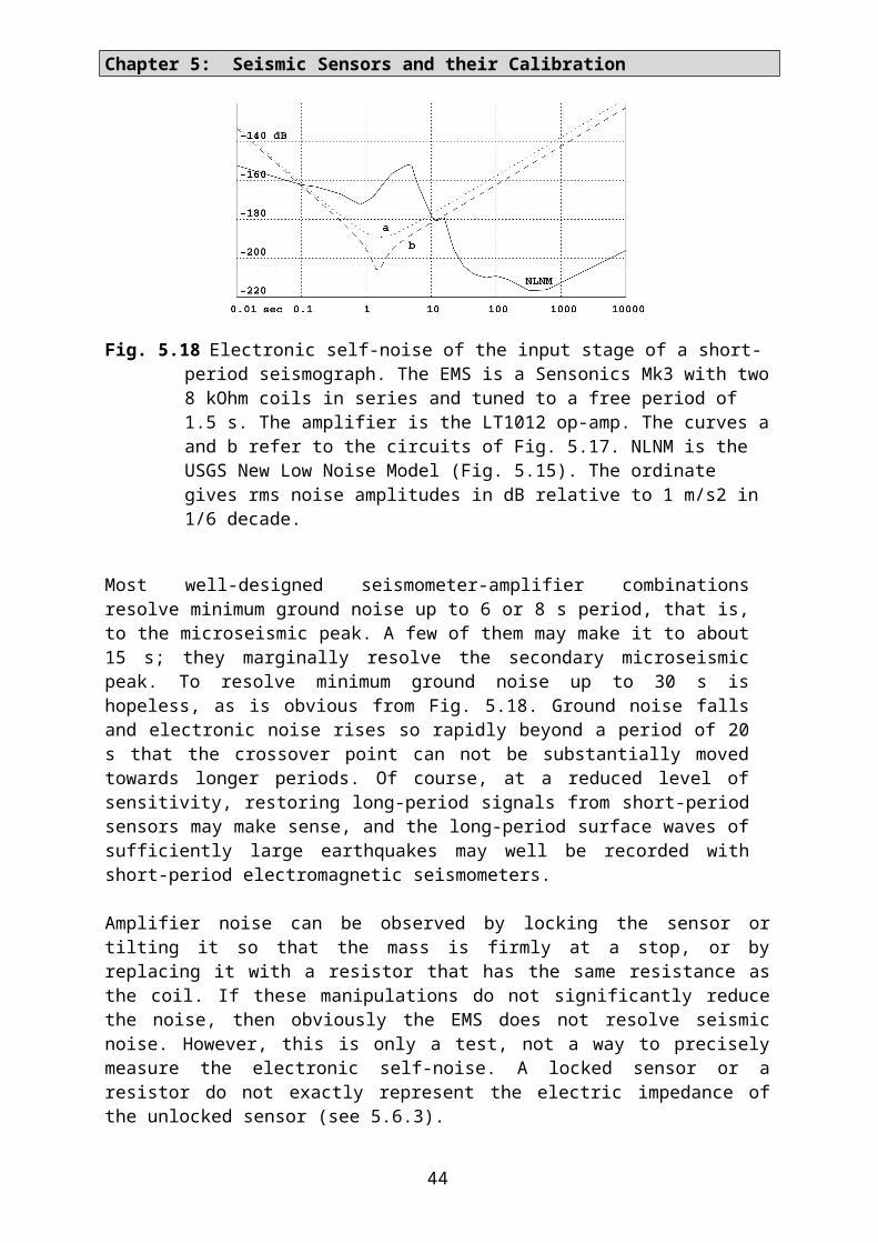
5.8 Free SoftwareSource codes and DOS executables of the computer programs CALEX, DISPCAL, POLZERO, RECTAX, SINCAL, SINFIT, TILTCAL, TRIAX, TRICROSP, TWOCROSP, and many others can be downloaded from the siteshttp://www.software-for-seismometry.de/ (this site always has the latest versions)http://www.geophys.uni-stuttgart.de/~erhard/downloads/ (a mirror site)Some programs of tutorial character are also found there (FOURIERDEMO, FILTDEMO, SURFER). Test data are supplied with most programs. Use the “software overview” on the website to select what you need, and read the “program descriptions” for details.
AcknowledgmentsThis is a revised version (May 2010) of Chapter 5 of the printed first edition of the IASPEI New Manual of Seismological Observatory Practice. The complete citation of the 2002 edi-tion is: New Manual of Seismological Observatory Practice (NMSOP), Volume 1&2, Editor: Peter Bormann. GeoForschungsZentrum Potsdam, 2002. ISBN 3-9808780-0-7.
Three careful reviews by the Editor of the NMSOP, Peter Bormann, and suggestions by Axel Plešinger and Jens Havskov have significantly improved the clarity and completeness of this text. A shorter version, with some advanced topics added, has appeared in part A of the IASPEI International Handbook of Earthquake and Engineering Seismology, ed. W. H. Lee et al., 2002, ISBN-13: 978-0-12-440652-0, ISBN-10: 0-12-440652-1.
5.9 References
Agnew et al. 1976 Agnew, D. C., Berger, J., Buland, R., Farrel, W. & Gilbert, F.: International deployment of accelerometers - a network for very long period seismology. EOS, 57(4), 180-188.
Agnew et al. 1986 Agnew, D. C., Berger, J., Farrell, W. E., Gilbert, J. F., Masters, G. & Miller, D.: Project IDA: A decade in review. EOS, 67(16), 203-212.
Anderson & Wood 1925 Anderson, J. A. & Wood, H. O.Description and theory of the torsion seismometer, Bull. Seism. Soc. Am., 15(1), 72p.
Beauduin et al. 1996 Beauduin, R., Lognonné, P., Montagner, J. P., Cacho, S., Karczewski, J. F. & Morand, M.The effects of the atmospheric pressure changes on seismic signals, Bull. Seism. Soc. Am., 86(6), 1760-1769.
Benioff & Press 1958
Benioff, H. & Press, F.Progress report on long period seismographs, Geophys. J. R. astr. Soc., 1(1), 208-215.
Berger et al. 2004Berger, J., Davis, P., Ekström, G. Ambient Earth noise: A survey of the Global Seismographic NetworkJ. Geophys. Res., 109, B11307, doi:10.1029/2004JB003408.
Berlage Jr. 1932 Berlage Jr., H. P., Seismometer, vol. 4 of Handbuch der Geophysik (ed. B. Gutenberg), chap. 4, pp. 299 - 526. Gebrueder Borntraeger Verlag, Berlin.
Block & Moore 1970 Block, B. & Moore, R. D.Tidal to seismic frequency investigations with a quartz accelerometer of new geometry, J. Geophys. Res., 75(18), 4361-4375.
Bormann 2002Bormann, P. (editor)IASPEI New Manual of Seismological Observatory Practice, ed. P. Bormann, ISBN 3-9808780-0-7, GeoForschungsZentrum Potsdam 2002
Bracewell 1978 Bracewell, R. N., The Fourier transformation and its applications. McGraw-Hill, New York, 2nd edn.
Buttkus 1986 Buttkus, B. (editor)Ten years of the Graefenberg array, vol. 35 of Geologisches Jahrbuch Reihe E. Bundesanstalt für Geowissenschaften und Rohstoffe, Hannover.
Cooley and Tukey 1965Cooley, J. S. and Tukey, J. W., An algorithm for the calculation of complex Fourier series. Math. Comp., 19, 297-301.
de Quervain & Piccard 1924 de Quervain, A. & Piccard, A., Beschreibung des 21-Tonnen-Universal-Seismographen System de Quervain - Piccard, Jahresber. Schweiz. Erdbebendienst, 1924.
Davis & Berger 2007Davis, P and Berger, J.Calibration of the Global Seismographic Network Using TidesSeismological Research Letters; July/August 2007; v. 78; no. 4; p. 454-459; DOI: 10.1785/gssrl.78.4.454
de Quervain & Piccard 1927 de Quervain, A. & Piccard, A., Déscription du séismographe universel de 21 tonnes système de Quervain-Piccard, Publ. Bureau Centr. Séism. Int. Sér. A, 4(32).
Dewey & Byerly 1969
Seismic Sensors and their Calibration: Testing for nonlinear distortions
Dewey, J. & Byerly, P., The early history of seismometry (to 1900), Bull. Seism. Soc. Am., 59(1), 183 - 227.
Ewing 1884Ewing, J. A., Measuring earthquakes, Nature, 30, 149-152, 174-177.
Forbriger 2007Forbriger, Th., Reducing magnetic field induced noise in broad-band seismic recordings. Geophys. J. Int. (2007) 169, 240–258.
Forbriger et al. 2008Forbriger, T., Widmer-Schnidrig, R., Wielandt, E., Hayman, M., and Ackerley, N., Magnetic field background variations can limit the sensitivity of seismic broad-band sensorshttp://www.rz.uni-karlsruhe.de/~bi77/download/paperware/Poster/PosterDGG08.pdf
Forbriger 2009Forbriger, Th., About the non-unique sensitivity of pendulum seismometers to translational, angular, and centripetal acceleration. Manuscript accepted for publication in the BSSA spe-cial issue on rotational seismology, to appear in 2009
Galitzin 1914Galitzin, B., Vorlesungen über Seismometrie. B. G. Täubner, Leipzig and Berlin.
Gal´perin 1955Gal´perin, E.I., Azimutal´nij metod sejsmiceskich nabludenij. Gostoptechizdat, 80 pp.
Gal´perin 1977Gal'perin, E. I., Polyarizationnyi metod seismicheskikh isledovanii. Nedra Press, Moscow.
Harjes & Seidl 1978Harjes, H.-P. & Seidl, D., Digital recording and analysis of broadband seismic data at the Graefenberg array, J. Geophys., 44, 511 - 523.
Havskov & Alguacil 2004Havskov, J. & Alguacil, G., Instrumentation in Earthquake Seismology. Modern Approaches in Geophysics vol. 22, ISBN 1402029683, Springer Verlag 2004
Holcomb 1989.Holcomb, G. L., A direct method for calculating instrument noise levels in side-by-side seis-mometer evaluations. Open-file report 89-214, U. S. Geological Survey.
Holcomb 1990Holcomb, G. L., A numerical study of some potential sources of error in side-by-side seis-mometer evaluations. Open-file report 90-406, U. S. Geological Survey.
Holcomb & Hutt 1992 Holcomb, L. G. & Hutt, C. R., An evaluation of installation methods for STS-1 seismometers.
Open File Report 92-302, U. S. Geological Survey, Albuquerque, New Mexico.
Hutt et al. 2009Hutt, C. R., Evans, J. R., Followill, F., Nigbor, R. L., and Wielandt, E., Guidelines for Stan-dardized Testing of Broad-band Seismometers and Accelerometers. U.S. Geological Survey Open File Report 2009-1295, Geological Survey, Albuquerque, New Mexico. 62p.Online publication: http://pubs.usgs.gov/of/2009/1295/
IRIS 1985 The design goals for a new global seismographic network. Incorporated Research Institutions for Seismology, Washington, DC.
Jones & Richards 1973 Jones, R. V. & Richards, J. C. S., The design and some applications of sensitive capacitance micrometers, Journal of Physics E: Scientific Instruments, 6, 589-600.
Knothe 1963Knothe, Ch., Verbesserte Auswertung tiefenseismischer Beobachtungen durch Verwendung von Mehrkomponenten-Stationen. Freiberger Forschungshefte, D149, 53 pp.
LaCoste 1934 LaCoste, L. J. B., A new type long period seismograph, Physics, 5, 178-180.
Lehner 1959 Lehner, F. E., An ultra long-period seismograph galvanometer, Bull. Seism. Soc. Am., 49(4), 399-401.
Melton 1981a Melton, B. S.,Earthquake seismograph development: a modern history -- part 1, EOS, 62(21), 505 - 510.
Melton 1981b Melton, B. S., Earthquake seismograph development: a modern history -- part 2, EOS, 62(25), 545 - 548.
Melton & Kirkpatrick 1970 Melton, B. S. & Kirkpatrick, B. M., The symmetric triaxial seismometer - its design for ap-plication in long-period seismometry, Bull. Seism. Soc. Am., 60(3), 717-739.
Miller 1963 Miller, W. F., The caltech digital seismograph, J. Geophys. Res., 68(3), 841 - 847.
Mitronovas & Wielandt 1975 Mitronovas, W. & Wielandt, E., High-precision phase calibration of long-period electromag-netic seismographs, Bull. Seism. Soc. Am., 65(2), 441-424.
Oliver & Murphy 1971 Oliver, J. & Murphy, L., WWNSS: Seismology's global network of observing stations, Sci-ence, 174, 254-261.
Oppenheim & Schafer 1999, 2009
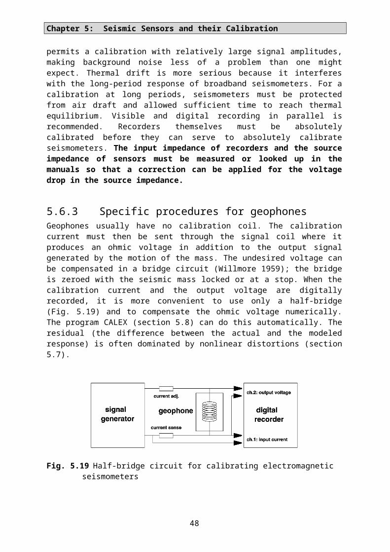
Seismic Sensors and their Calibration: Testing for nonlinear distortions
Oppenheim, A. V., Schafer, R. V., Buck, J.R., Discrete-Time Signal Processing, 2nd edition 1999 , 3rd edition 2009, Prentice-Hall, New Jersey, USA
Oppenheim & Willsky 1983 Oppenheim, A. V. & Willsky, A. S., Signals and Systems. Prentice Hall, New Jersey, USA.
Passcal Instrument Center 2009 a,bAnonymous, Broadband Vault Construction (Manual),http://www.passcal.nmt.edu/content/broadband-vault-construction-manualAnonymous, Seismic Vaults, http://www.passcal.nmt.edu/content/seismic-vaults
Pavlis & Vernon 1994 Pavlis, G. L. & Vernon, F. L., Calibration of seismometers using ground noise, Bull. Seism. Soc. Am., 84(4), 1243 - 1255.
Peterson 1993 Peterson, J., Observations and modelling of background seismic noise. Open File report 93-322, U. S. Geological Survey, Albuquerque, New Mexico. Peterson et al. 1976
Peterson et al. 1976Peterson, J., Butler, H. M., Holcomb, L. G. & Hutt, C. R., The seismic research observatory, Bull. Seism. Soc. Am., 66(6), 2049-2068.
Peterson et al. 1980Peterson, J., Hutt, C. R. & Holcomb, L. G., Test and calibration of the seismic research ob-servatory. Open File report 80-187, U. S. Geological Survey, Albuquerque, New Mexico.
Plesinger and Horalek 1976Plesinger, A. & Horalek, J., The seismic broad-band recording and data processing system FBS/DPS and its seismological applications, J. Geophys., 42, 201 - 217. Plesinger et al. 1996 Plesinger, A., Zmeskal, M. & Zednik, J., Automated preprocessing of digital seismograms: Principles and software. E. Bergman (ed.), Prague and Golden, Prague.
Press et al. 1958 Press, F., Ewing, M. & Lehner, F., A long-period seismograph system, Trans. Am. Geophys. Union, 39(1), 106-108.
Riedesel et al. 1990 Riedesel, M. A., Moore, R. D. & Orcutt, J. A., Limits of sensitivity of inertial seismometers with velocity transducers and electronic amplifiers, Bull. Seism. Soc. Am, 80(6), 1725 - 1752.
Robinson & Treitel 1980 Robinson, E. A. & Treitel, S., Geophysical Signal Analysis. Prentice-Hall, New York.
Rodgers 1968 Rodgers, P. W., The response of the horizontal pendulum seismometer to Rayleigh and Love waves, tilt, and free oscillations of the Earth, Bull. Seism. Soc. Am., 58(5), 1385-1406.
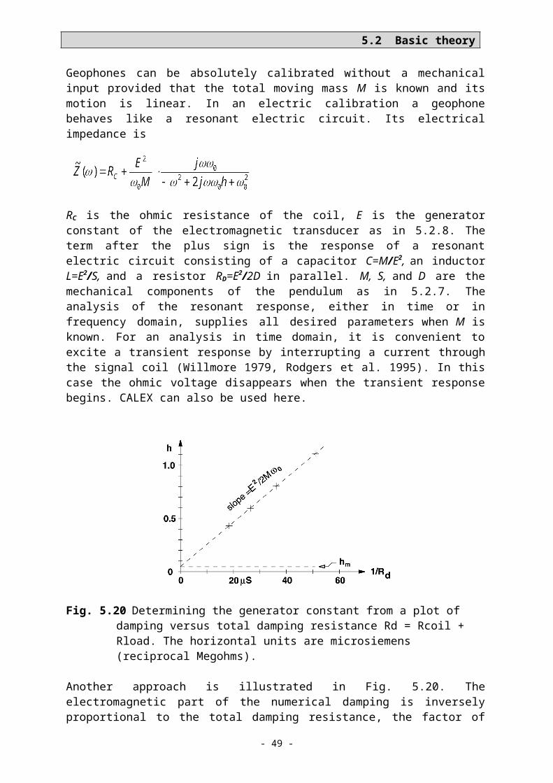
Rodgers 1969 Rodgers, P. W., A note on the response of the pendulum seismometer to plane wave rotation, Bull. Seism. Soc. Am., 59(5), 2101-2102.
Rodgers 1992Rodgers, P. W., Frequency limits for seismometers as determined from signal-to-noise ratios. Part 1: the electromagnetic seismometer, Bull. Seism. Soc. Am., 82(2), 1071-1098.
Rodgers 1993 Rodgers, P. W., Maximizing the signal-to-noise ratio of the electromagnetic seismometer: the optimum coil resistance, amplifier characteristics, and circuit., Bull. Seism. Soc. Am., 83(2), 561-582.
Rodgers et al. 1995 Rodgers, P. W., Martin, A. M., Robertson, M. C., Hsu, M. M. & Harris, D. B., Signal-coil calibration of electromagnetic seismometers, Bull. Seism. Soc. Am., 85(3), 845-850.
Savino et al. 1972 Savino, J. M., Murphy, A. J., Rynn, J. M. W., Tatham, R., Sykes, L. R., Choy, G. L. & Mc-Camy, K., Results from the high-gain long-period seismograph experiment, Geophys. J. R. astron. Soc., 31(1), 179-203.
Scherbaum 1996, 2007Scherbaum, F., Of Poles and Zeros, Fundamentals of Digital Seismology. Kluwer Academic, 1996. 2nd revised edition, Springer Verlag Berlin und Heidelberg
Schuessler 1981 Schuessler, H. W., A signalprocessing approach to simulation, Frequenz, 35, 174-184.
Sleeman et al. 2006Sleeman, R., van Wettum, A., Trampert, J., Three-channel correlation analysis: a new tech-nique to measure instrumental noise of digitizers and seismic sensors, Bull. Seism. Soc. Am., Vol. 96, No. 1, pp. 258-271, doi:10.1785/0120050032.
Tanimoto 1999 Tanimoto, T., Excitation of normal modes by atmospheric turbulence: source of long-period seismic noise, Geophys. J. Int., 136(2), 395-402.
Trnkoczy 1998 Trnkoczy, A., Guidelines for civil engineering works at remote seismic stations. Application Note 42, Kinemetrics Inc., 222 Vista Av., Pasadena, Ca. 91107. http://www.kinemetrics.com/eng_ftp/AppNotes/appnote42.PDF
Uhrhammer & Karavas 1997 Uhrhammer, R. A. & Karavas, W., Guidelines for installing broadband seismic instrumenta-tion. Tech. rep., Seismographic station, University of California at Berkeley, http://seismo.berkeley.edu/bdsn/instrumentation/guidelines.html
Usher et al. 1978
Seismic Sensors and their Calibration: Testing for nonlinear distortions
Usher, M. J., Guralp, C. & Burch, R. F., The design of miniature wideband seismometers, Geophys. J., 55(3), 605 - 613.
Von Rebeur-Paschwitz 1889 Von Rebeur-Paschwitz, E., The earthquake of Tokyo, April 18, 1889, Nature, 40, 294-295.
Wielandt 1975 Wielandt, E., Ein astasiertes Vertikalpendel mit tragender Blattfeder, J. Geophys., 41(5), 545 - 547.
Wielandt 1983 Wielandt, E., Design principles of electronic inertial seismometers. In Earthquakes: Observa-tion, Theory and Interpretation, pp. 354-365. LXXXV Corso, Soc. Italiana di Fisica, Bologna.
Wielandt & Forbriger 1999 Wielandt, E. & Forbriger, T., Near-field seismic displacement and tilt associated with the ex-plosive activity of Stromboli, Annali di Geofisica, 42(2 or 3).
Wielandt & Steim 1986 Wielandt, E. & Steim, J. M., A digital very-broad-band seismograph, Annales Geophysicae, 4 B(3), 227-232.
Wielandt & Streckeisen 1982 Wielandt, E. & Streckeisen, G., The leaf-spring seismometer: design and performance, Bull. Seism. Soc. Am., 72(6), 2349-2367.
Willmore 1959 Willmore, P. L., The application of the Maxwell impedance bridge to the calibration of elec-tromagnetic seismographs, Bull. Seism. Soc. Am., 49(1), 99-114.
Willmore 1979 Willmore, P. L. (editor), Manual of seismological observatory practice. Tech. Rep. SE-20, World data center A for solid earth geophysics, NOAA, Boulder, Color-ado 80303, USA.
Zürn & Widmer 1995 Zürn, W. & Widmer, R., On noise reduction in vertical seismic records below 2 mHz using local barometric pressure, Geophys. Res. Lett., 22(24), 3537-3540.