466 ieee transactions on evolutionary...
TRANSCRIPT
466 IEEE TRANSACTIONS ON EVOLUTIONARY COMPUTATION, VOL. 11, NO. 4, AUGUST 2007
Natural Encoding for EvolutionarySupervised Learning
Jesús S. Aguilar-Ruiz, Raúl Giráldez, and José C. Riquelme
Abstract—Some of the most influential factors in the quality ofthe solutions found by an evolutionary algorithm (EA) are a cor-rect coding of the search space and an appropriate evaluation func-tion of the potential solutions. EAs are often used to learn decisionrules from datasets, which are encoded as individuals in the ge-netic population. In this paper, the coding of the search space forthe obtaining of those decision rules is approached, i.e., the rep-resentation of the individuals of the genetic population and alsothe design of specific genetic operators. Our approach, called “nat-ural coding,” uses one gene per feature in the dataset (continuousor discrete). The examples from the datasets are also encoded intothe search space, where the genetic population evolves, and there-fore the evaluation process is improved substantially. Genetic op-erators for the natural coding are formally defined as algebraicexpressions.
Experiments with several datasets from the University ofCalifornia at Irvine (UCI) machine learning repository show thatas the genetic operators are better guided through the searchspace, the number of rules decreases considerably while main-taining the accuracy, similar to that of hybrid coding, which joinsthe well-known binary and real representations to encode discreteand continuous attributes, respectively. The computational costassociated with the natural coding is also reduced with regard tothe hybrid representation.
Our algorithm, HIDER*, has been statistically tested againstC4.5 and C4.5 Rules, and performed well. The knowledge modelsobtained are simpler, with very few decision rules, and thereforeeasier to understand, which is an advantage in many domains.The experiments with high-dimensional datasets showed the samegood behavior, maintaining the quality of the knowledge modelwith respect to prediction accuracy.
Index Terms—Decision rules, evolutionary encoding, supervisedlearning.
I. INTRODUCTION
DECISION RULES are especially relevant in problems re-lated to supervised learning. Given a dataset with contin-
uous and discrete features or attributes, and a class label, we tryto find a rule set that describes the knowledge within data orclassifies new unseen data. When the feature is discrete, therules take the form of “if , then class,” wherethe values are not necessarily all those that the fea-ture can take. When the feature is continuous, typically therules take the form of “if then class,” where
Manuscript received December 18, 2005; revised April 22, 2006. This workwas supported in part by the Spanish Research Agency CICYT under GrantTIN2004-00159 and in part by Junta de Andalucía (III Research Plan).
J. S. Aguilar-Ruiz and R. Giráldez are with the School of Engineering,Pablo de Olavide University, 41013 Seville, Spain (e-mail: [email protected];[email protected]).
J. C. Riquelme is with the Department of Computer Science, University ofSeville, 41004 Seville, Spain (e-mail: [email protected]).
Digital Object Identifier 10.1109/TEVC.2006.883466
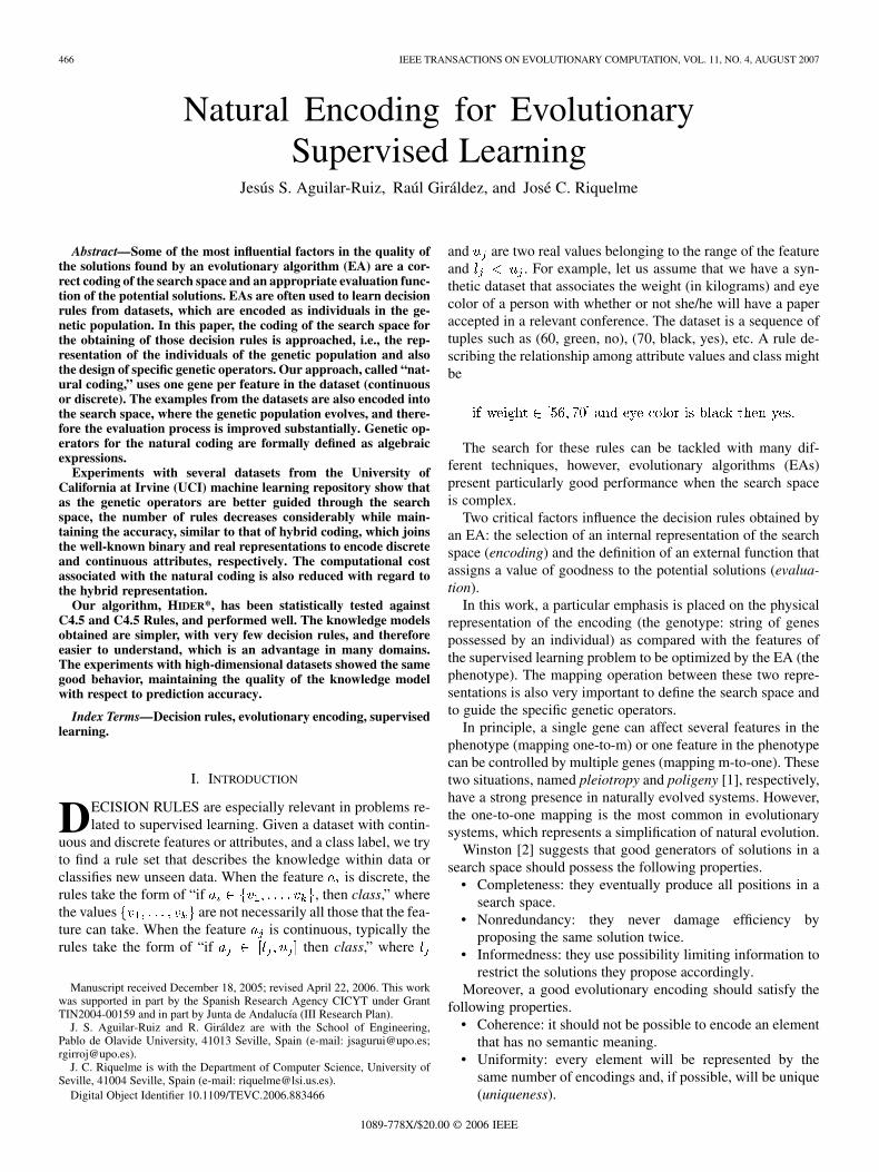
and are two real values belonging to the range of the featureand . For example, let us assume that we have a syn-thetic dataset that associates the weight (in kilograms) and eyecolor of a person with whether or not she/he will have a paperaccepted in a relevant conference. The dataset is a sequence oftuples such as (60, green, no), (70, black, yes), etc. A rule de-scribing the relationship among attribute values and class mightbe
The search for these rules can be tackled with many dif-ferent techniques, however, evolutionary algorithms (EAs)present particularly good performance when the search spaceis complex.
Two critical factors influence the decision rules obtained byan EA: the selection of an internal representation of the searchspace (encoding) and the definition of an external function thatassigns a value of goodness to the potential solutions (evalua-tion).
In this work, a particular emphasis is placed on the physicalrepresentation of the encoding (the genotype: string of genespossessed by an individual) as compared with the features ofthe supervised learning problem to be optimized by the EA (thephenotype). The mapping operation between these two repre-sentations is also very important to define the search space andto guide the specific genetic operators.
In principle, a single gene can affect several features in thephenotype (mapping one-to-m) or one feature in the phenotypecan be controlled by multiple genes (mapping m-to-one). Thesetwo situations, named pleiotropy and poligeny [1], respectively,have a strong presence in naturally evolved systems. However,the one-to-one mapping is the most common in evolutionarysystems, which represents a simplification of natural evolution.
Winston [2] suggests that good generators of solutions in asearch space should possess the following properties.
• Completeness: they eventually produce all positions in asearch space.
• Nonredundancy: they never damage efficiency byproposing the same solution twice.
• Informedness: they use possibility limiting information torestrict the solutions they propose accordingly.
Moreover, a good evolutionary encoding should satisfy thefollowing properties.
• Coherence: it should not be possible to encode an elementthat has no semantic meaning.
• Uniformity: every element will be represented by thesame number of encodings and, if possible, will be unique(uniqueness).
1089-778X/$20.00 © 2006 IEEE
AGUILAR-RUIZ et al.: NATURAL ENCODING FOR EVOLUTIONARY SUPERVISED LEARNING 467
• Simplicity: the coding function must have easy applicationin both directions.
• Locality: small modifications to the values (phenotype)should correspond to small modifications to the hypothet-ical solutions (genotype).
• Consistency: futile or unproductive codings should notexist .
• Minimality: the length of the coding should be as short aspossible.
On the other hand, internal redundancy should be avoided.A representation is said to contain internal redundancy whennot all of the genetic information contained in a chromosomeis strictly necessary in order to identify uniquely the solution towhich it corresponds. It is also very common to find degeneracyin representations. A representation is said to exhibit degeneracywhen more than one chromosome can represent the same so-lution. Degeneracy is often detrimental to genetic search [3],because it means that isomorphic forms are allowed. In someproblems, the effect of one gene suppresses the action of one ormore other genes. This feature of interdependency, called epis-tasis, should also be controlled and minimized.
Therefore, the design of a new representation for EAs is notsimple if we wish it to have a good performance. In fact, not onlyshould the encoding preserve most of the properties mentionedabove, but new genetic operators should also provide some ad-vantages when the new encodings are used. In this work, wepresent a new evolutionary encoding to produce decision rules.Our approach, named “natural coding,” is a one-to-one map-ping, and it only uses natural numbers to encode continuousand discrete features. This coding needs a new definition for thegenetic operators in order to avoid the conversion from naturalnumbers to the values in the original space. These definitionsare presented, and as it is shown in this paper, the EA can workdirectly with the natural coding until the end, when the individ-uals will be decoded to decision rules.
This paper is organized as follows: in Section II, the workrelated to binary, integer, and real codings is presented; the mo-tivation of our approach is described in Section III; the naturalcoding is presented in Section IV, together with the genetic op-erators associated with continuous and discrete attributes; thealgorithm is illustrated in Section V, discussing the new eval-uation method and the length of individuals; later, we com-pare our approach to the hybrid coding regarding the lengthof individuals and to C4.5 and C4.5 Rules to search for statis-tical differences about the error rate and the number of rules inSection VI; finally, the most interesting conclusions are summa-rized in Section VII.
II. RELATED WORK
Choosing a good genetic representation is critical for the EAto find a good solution for the problem because the encodingwill have much influence on achieving an effective search. Bi-nary, Gray, and floating-point chromosome encodings have beenwidely used in the literature because they have provided gener-ally satisfactory results. Thus, few alternatives have been ana-lyzed. Nevertheless, there are many ways of associating featurevalues to genes, which should be discussed in light of findingthe best one for specific problems.
Taking the aforementioned properties into account, we aregoing to analyze the most common representations for EAs,from the perspective of supervised learning. To our knowledge,little theoretical work has been developed in the field of evolu-tionary encoding. Many authors have approached several cod-ings for specific applications, most of them for optimization orscheduling tasks, clustering, and feature selection. However, insupervised learning, the binary, real and hybrid (binary codingfor discrete features and real for continuous) codings have com-manded the attention of many researchers.
A number of studies dedicated to EAs, beginning with Hol-land’s [4] made use of binary coding. The simplicity and, aboveall, the similarity with the concept of Darwinian analogy, haveadvanced its theoretical use and practical application. Severalgenetic algorithms-based concept learners apply binary codingto encode features with symbolic domains in order to inducedecision rules in either propositional (GABIL [5], GIL [6],COGIN [7]) or first-order form (REGAL [8], [9], and DOGMA[10]). However, binary coding is not the most appropriate forcontinuous domains.
In general, binary coding has been widely used, for instance,for feature selection [11] and data reduction [12].
In general, assuming that the interaction among attributes isnot linear, in principle, the size of the search space is related tothe number of genes used. For an individual with genes, thesize of the search space is , where is the alphabetfor the th gene. Traditionally, the same alphabet has been usedfor every gene, mostly the binary alphabet, so that .However, for a continuous feature with range , if we decideto use length to encode it, the error in the precision of thatattribute would be
(1)
Therefore, if ,the minimum encoding length, to ensure the precision is main-tained, would be
(2)
Taking into account (2), the quantum defined by error willassure that the length is the least that guarantees a good preci-sion for the mutation operator. However, the locality problem isnot solved for binary representation. Gray encoding, where twoindividuals next to each other in the search space differ by onlyone bit, has been studied in depth [13], [14] and offers some ad-vantages in this realm [15], although it suffers from the samelack of precision as binary coding.
Both binary and Gray representations have some drawbackswhen applied to multidimensional, high-precision problems.For example, for ten attributes with domains in the range [0,1],where a precision of three digits after the decimal point isrequired, the length of an individual is about 100. This, in turn,generates a search space size of about .
For many problems, binary and Gray encoding are not ap-propriate because a value of 1 bit may suppress the fitness con-tributions of other bits in the genotype (epistasis) and geneticoperators may produce illegal solutions (inconsistency). Some
468 IEEE TRANSACTIONS ON EVOLUTIONARY COMPUTATION, VOL. 11, NO. 4, AUGUST 2007
examples of other specific encodings are: Prüfer numbers to rep-resent spanning trees [16] and integer numbers to obtain hierar-chical clusters [17].
In real-valued coding [18], the chromosome is encoded asa vector of floating-point numbers of the same length as thesolution vector. Each attribute is forced to be within a desiredrange and the operators are carefully designed to preserve thisrequirement. The motivation behind floating-point codings is tomove the EA closer to the problem space. This coding is capableof representing quite large domains.
On the contrary, its main theoretical problem is the size ofthe search space. Since the size of the alphabet is infinite, thenumber of possible schemes is also infinite and, therefore, manyschemes that are syntactically different but semantically similarwill coexist (degeneracy).
In principle, any value can be encoded with an only (real)gene, but this could be avoided by using a discrete search space,where the mapping is one-to-one. However, instead of mappingreal values to real values, we will map natural numbers to realintervals. For continuous domains, the intervals can preciselydefine a range of values within the domain. With this solution,the size of the search space is finite, and therefore so is thenumber of schemes as well. However, this search space reduc-tion requires a prior discretization of continuous attributes, sothe choice of the discretization method is critical. This idea willbe explained in detail in Section IV-B.
The approaches gathered in the bibliography, some of thembased on evolutionary strategies, use real coding for machinelearning tasks [19] or for multiobjective problems [20]. In SIA[21], real coding is applied to a real-world data analysis taskin a complex domain. Finally, a combination of binary and realcoding is used in [22] in order to benefit from the advantages ofboth codings by using the binary approach in discrete domainsand real coding for continuous attributes.
Fuzzy coding is another alternative for representing a chro-mosome. Every attribute consists of a fuzzy set and a set ofdegrees of membership to each fuzzy set [23]. Some other en-coding strategies have been used in EAs. These include trees,matrix encodings, permutation encodings, and structured het-erogeneous encodings to name a few.
III. MOTIVATION
The main shortcoming of using real coding to produce deci-sion rules is that any value in the range of the attribute couldbe used as lower or upper bound of the interval for that attributecondition. For example, the C4.5 tool [25] only takes as possiblevalues for the nodes of the decision trees the midpoints amongtwo consecutive values of an attribute. This idea might be usedto encode an individual of the genetic population so that onlyhypothetically good values will be allowed as conditions overan attribute in the rules. In a similar way, Bonissone et al. showin [24] some real-world applications where the knowledge ofthe problem domain benefits the use of EAs.
To clarify this idea, we will use the dataset shown in Fig. 1,whose features are described in Section I. Observing the at-tribute weight (the first one), C4.5 would investigate as possiblevalues: 56, 58, 59.5, 61, 63, 66, and 69. In other words, C4.5is applying a local unsupervised method of discretization [26]
Fig. 1. Labeled dataset with one continuous and one discrete attribute.
since the class label is not taken into account in this process.The reduction of the number of values is only determined bythe number of equal values for the attribute being considered.This unsupervised discretization is not a good choice to analyzepossible limit values (either using entropy or any other criterion)for the intervals [27].
A number of remarkable supervised discretization methodshave been included in the bibliography, including Holte’s 1R[28] and the method of Fayyad and Irani [29]. In [30], a super-vised discretization method, named unparametrized superviseddiscretization (USD) is presented. This method is very similarto 1R, although it does not need any input parameter. However,as the aim of this method is not to find intervals but cutpointsto be used as limits of further decision rules, we assume thatany supervised discretization method would be appropriate forthis purpose. As we will see below, if the discretization methodproduces cutpoints, then there will be possibleintervals for the decision rules.
Our goal consists in observing the class along with the dis-cretization method and decreasing the alphabet size. Followingthe example in Fig. 1, we can note that it is only necessary to in-vestigate the values 56, 61, 63, and 66, because they are valueswhich produce a change of class. Therefore, this coding allowsthe use of all the possible intervals defined by every pair of cut-points obtained by means of discretization, together with thefeature range bounds.
In short, if we are able to encode every possible interval andevery possible combination of discrete values in such a way thatthe genetic operators make an efficient search of potential solu-tions, then the proposed representation will be appropriate forour purpose. Next, we are going to present and discuss this newencoding method, which will disclose interesting properties.
The natural coding leads to a reduction of the search spacesize, which has a positive influence on the convergence of theEA with respect to the hybrid coding HIerarchical DEcisionRules (HIDER [22]). The prediction accuracy is maintained,while the number of rules is decreased, therefore using lesscomputational resources.
IV. NATURAL CODING
In this section, we propose a new encoding for EAs in orderto find decision rules in the context of supervised learning, to-gether with their genetic operators, which will be presented intwo independent subsections: discrete and continuous features,respectively. This coding has been named “natural” because it
AGUILAR-RUIZ et al.: NATURAL ENCODING FOR EVOLUTIONARY SUPERVISED LEARNING 469
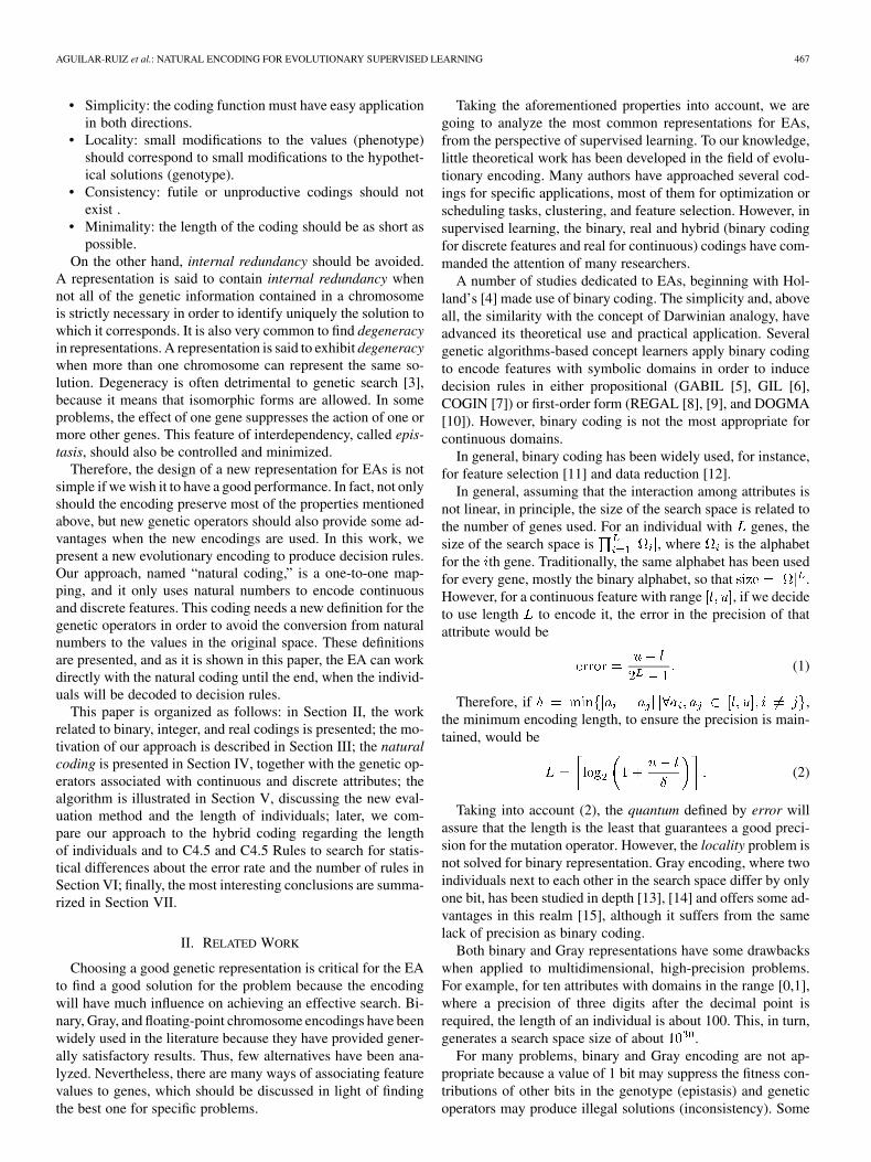
Fig. 2. Hybrid individual versus natural individual.
only uses natural numbers to represent the set of intervals forcontinuous features and the set of values for discrete ones, whichmight take part in the decision rules.
Regarding the properties mentioned in Section I, naturalcoding is complete, nonredundant, and informed. The internalredundancy and degeneracy properties are especially taken intoaccount to perform an effective search for solutions. Moreover,it is coherent, unique, simple, consistent, and minimal. Localityis also satisfied as small variations of the natural numbers cor-respond to small modifications of the intervals they represent.
Through the text, we will use a very simple dataset in orderto explain the application of the genetic operators. This dataset(see Fig. 1) has a continuous attribute (weight in kilograms)with range [55, 70], a discrete attribute (eye color) with values
black, green, blue , and a class (she/he is a candidate to have apaper accepted in a relevant conference) with values yes, no .Although the semantics of the natural coding have not yet beendetailed, Fig. 2 illustrates the length of natural versus hybridrepresentations. It shows two individuals that represent the samerule. The method to encode these values will be shown later.
Hybrid coding represents a rule comprising the union of twotypes of genotypes: real coding for the continuous attributes andbinary coding for the discrete ones. Each condition associatedwith a continuous attribute is encoded by two real numbers rep-resenting the bounds of the interval for that attribute. Each con-dition related to a discrete feature is encoded by a vector of bi-nary values. The size of this vector is equal to the number of dis-tinct values of the attribute, so that 1 means that attribute valueis present in the condition, and 0, absent. For instance, the rulein Fig. 2 is encoded by using the hybrid coding (left).
The main problem of this encoding is that the search spaceis very large, since for each continuous feature we have to findtwo values in the range of the attribute. Another drawback is thelength of the individuals, which might be very large when thediscrete attributes take many distinct values. Our proposal triesto minimize the search space size and the length of the indi-viduals by assigning only one natural number to each conditionregardless of the type of the attributes. Thus, we attempt to limitthe search space of valid genotypes and reduce the length of theindividuals. When the attributes are discrete, this natural numberis the conversion of the aforementioned binary string from thehybrid coding into a decimal number. For continuous features,the natural number is obtained by numbering all the possibleintervals the condition can represent in an effective manner.
In Fig. 2, a rule is encoded by the natural encoding (right), incontrast with the hybrid encoding (left). In this genotype, themeaning of 8 is the number assigned to the interval [56, 63] inthe set of all valid intervals for , and the number 5 is theinteger that represents the binary string 101 for .
We can note that the natural coding is simpler, since the hy-brid coding needs six genes to encode the rule, whereas the nat-ural one encodes it with only three genes. In general, the hybridone uses two genes for continuous features and for discreteones, where is the number of different values that the fea-ture can take. The natural coding gets to minimize the size ofindividuals, assigning only one gene to each feature.
In general, to choose an encoding and a suitable set of ge-netic operators is not an easy task. An unacceptable amount ofdisruption can be introduced to the phenotype as a result of theinappropriate design of genetic operators or the choice of the en-coding strategy. Sometimes degeneracy is seen as a beneficialeffect to incorporate additional information. However, it is notalways a positive phenomenon since the genetic operators mightnot increase the level of diversity of the next generation. In thiscase, the implicit parallelism would also be reduced. As a norm,encodings should be designed to naturally suppress redundantencoding forms, and genetic operators should be implementedin such a way that redundant forms do not benefit the operators.
A. Discrete Features
Several systems exist that learn concepts (concept learners)and use binary coding for discrete features. When the set of at-tribute values has many different values, the length of the indi-vidual is very high so that a reduction in length might have apositive effect on speeding the algorithm.
In the following discussions, we will assume that a discretefeature is encoded by a single natural number (one gene), andwe will analyze how to apply the crossover and mutation opera-tors such that the new values retain the meaning that they wouldhave had with a binary coding. The new value will belong to theinterval , where is the number of different valuesof the attribute. With the natural coding for discrete attributes, areduction of the size of the search space is not obtained by itself,but the individuals are better guided through the search space tolook for solutions when the specifically designed “natural ge-netic operators” are applied.
The natural coding is obtained from a binary coding similarto that used in GABIL and GIL. In decision rules, a conditioncan establish a set of discrete values that the feature must satisfyfor an example to be classified. If a value is included in thecondition, its corresponding bit is equal to 1, otherwise, it is 0.The natural coding for this gene is the conversion of the binarynumber into a natural number. Table I shows an example fora discrete feature with three different values: black, green, andblue.
1) Natural Mutation: Following the example in Table I,when a value is selected for mutation, for example, 3
, there are three options: 111, 001,and 010, equivalent to the numbers 7, 1, and 2, respectively.First, we assign the natural number corresponding to eachbinary number. The mutation of each value would have to be
470 IEEE TRANSACTIONS ON EVOLUTIONARY COMPUTATION, VOL. 11, NO. 4, AUGUST 2007
TABLE ICODING FOR A DISCRETE ATTRIBUTE
TABLE IIMUTATION VALUES FOR DISCRETE ATTRIBUTES
some of the values shown in Table II. For example, possiblemutations of 0 are the values 1, 2, and 4.
Definition 1 (Natural Mutation): Let be the value of a geneof an individual, then the natural mutation of the th bit of , de-noted by , is the natural number produced by changingthat th bit
% (3)
where is the number of values of theattribute; are the possible mutated values from ; % isthe rest of the integer division; and is the integer part.
Example 1: For example, according to Table II, the possiblemutation values for will be 4, 7, and 1
%
%
%
It is worth noting that we do not need to know the binaryvalues, as (3) takes a natural number and provides its naturalmutations.
Definition 2 (Mutation Set): Let be the value of a gene, wedefine mutation set, , as the set of all valid mutations fora natural value
(4)
where is the natural mutation of the th binary bit.Example 2: From Example 1, .Note that every discrete feature value set represented by a
natural number can be mutated by using (4), generating a setof natural numbers which represents new discrete feature valuesets. Therefore, binary values do not appear in the population.
As shown in Example 2, from the value , thepossible values are and
.2) Natural Crossover:Definition 3 ( -Order Mutation): Let be a set of natural
numbers, let us define the -order mutation, and it will be de-noted as , as follows:
...
(5)
Definition 4 (Natural Crossover): Let and be the valuesof two genes from two individuals for the same feature. The geneof the offspring will be obtained from the valuesbelonging to the first nonempty intersection between the -ordermutations. Let , and , then
(6)
Example 3: Let us assume that we have the values 6(110) and3(011). We include the current values into the mutation set sincethe offspring could be similar to the parents. Thus, 6 mutates to
and 3 mutates to . As both genes share2(010) and 7(111), any of them could be the offspring from 6and 3. It is possible that the intersection is the parents (for ex-ample, for 1 and 3, as the schema is the same for both, 0*1).
Example 4: Lets assume that we have the worst case, thevalues 1(001) and 6(110), which have no bits in common. Theintersection between the first two mutation sets is empty. Theprocess is shown next
The intersection will be , and any of them willbe the valid offspring for .
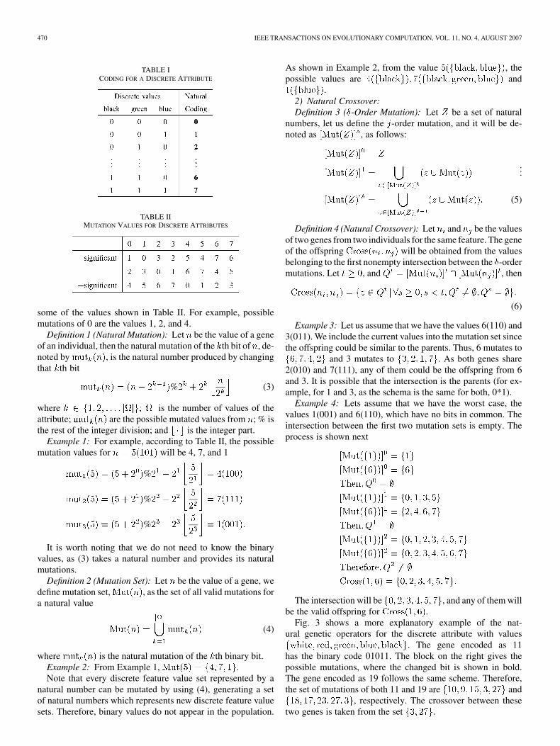
Fig. 3 shows a more explanatory example of the nat-ural genetic operators for the discrete attribute with values
. The gene encoded as 11has the binary code 01011. The block on the right gives thepossible mutations, where the changed bit is shown in bold.The gene encoded as 19 follows the same scheme. Therefore,the set of mutations of both 11 and 19 are and
, respectively. The crossover between thesetwo genes is taken from the set .
AGUILAR-RUIZ et al.: NATURAL ENCODING FOR EVOLUTIONARY SUPERVISED LEARNING 471
Fig. 3. Example of mutation and crossover operators for a discrete attribute with five values fwhite, red, green blue, blackg.
TABLE IIIINTERVALS CALCULATED FOR THE CONTINUOUS ATTRIBUTE WITH RANGE [55,70]. THE BOUNDARY POINTS ARE
f55; 56; 61; 63; 66;70g. A NATURAL NUMBER IS ASSOCIATED WITH EVERY CORRECT INTERVAL
B. Continuous Features
Using binary encoding in continuous domains requires trans-formations from binary to real for every feature in order to applythe evaluation function. Moreover, when we convert binary intoreal, the precision might be affected. Ideally, the mutation of theless significant bit of an attribute should include or exclude atleast one example from the training set. The real coding seemsmore appropriate with real domains, simply because it is morenatural to the domain. A number of authors have investigatednonbinary EAs theoretically [31]–[35]. In this sense, each genewould be encoded with a float value. Two float values would beneeded to express the interval of a continuous feature.
As the range of continuous attributes is infinite, it would beinteresting to reduce the search space size, as the computationalcost should be lower. This reduction should not have negativeinfluence on the prediction accuracy of the solutions (decisionrules) found by the EA. The first step, therefore, consists in di-minishing the cardinality of the set of values of the attribute.
1) Reducing the Cardinality: First, we will analyze what in-tervals inside the range of the attribute tend to appear as in-tervals for a potential decision rule obtained from the naturalcoding. As mentioned before, this task could be solved by anysupervised discretization algorithm. In [27], it is carried out viaan experimental evaluation of various discretization schemes indifferent evolutionary systems for inductive concept learning,where our tool with natural coding, named HIDER*, was also
analyzed. This study showed that HIDER* was robust for anydiscretization method [27, Table II], although USD [30] turnedout to be the most stable discretizer used in that experiment (thelast column in [27, Table IV]).
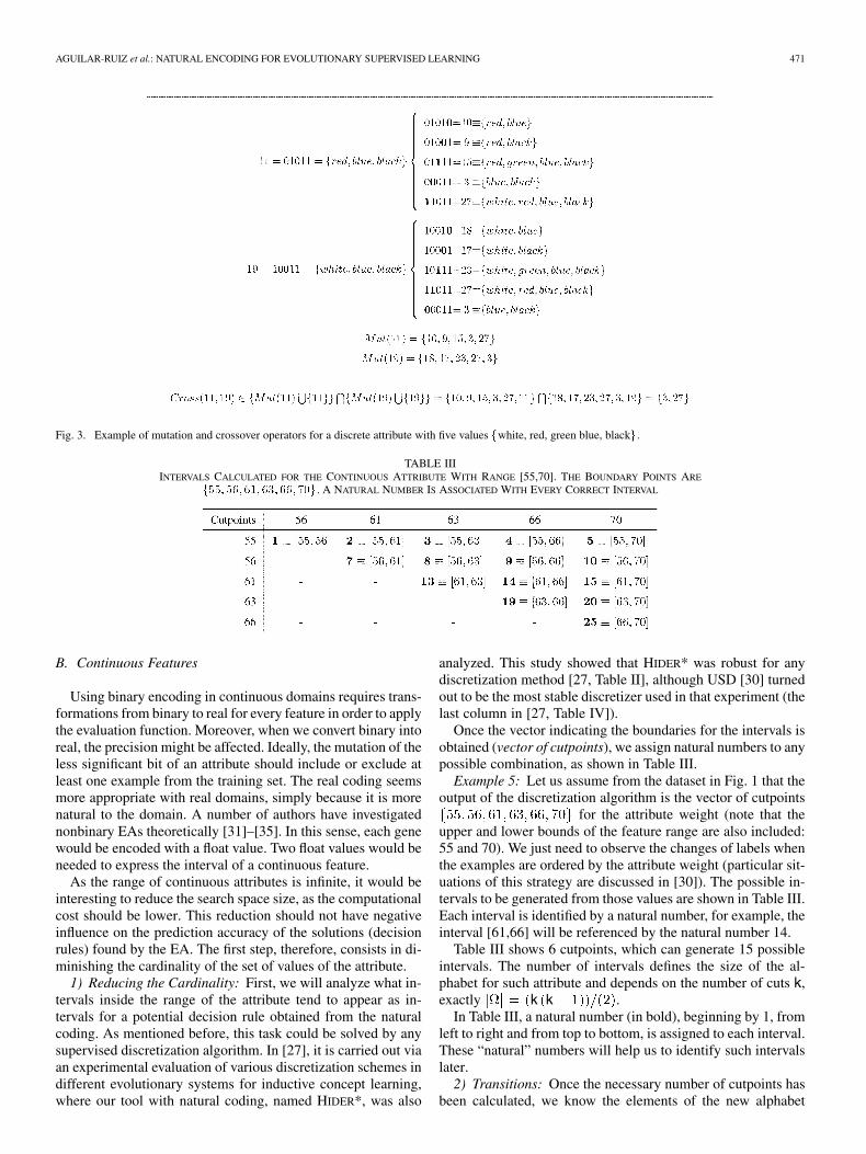
Once the vector indicating the boundaries for the intervals isobtained (vector of cutpoints), we assign natural numbers to anypossible combination, as shown in Table III.
Example 5: Let us assume from the dataset in Fig. 1 that theoutput of the discretization algorithm is the vector of cutpoints
for the attribute weight (note that theupper and lower bounds of the feature range are also included:55 and 70). We just need to observe the changes of labels whenthe examples are ordered by the attribute weight (particular sit-uations of this strategy are discussed in [30]). The possible in-tervals to be generated from those values are shown in Table III.Each interval is identified by a natural number, for example, theinterval [61,66] will be referenced by the natural number 14.
Table III shows 6 cutpoints, which can generate 15 possibleintervals. The number of intervals defines the size of the al-phabet for such attribute and depends on the number of cuts k,exactly k k .
In Table III, a natural number (in bold), beginning by 1, fromleft to right and from top to bottom, is assigned to each interval.These “natural” numbers will help us to identify such intervalslater.
2) Transitions: Once the necessary number of cutpoints hasbeen calculated, we know the elements of the new alphabet
472 IEEE TRANSACTIONS ON EVOLUTIONARY COMPUTATION, VOL. 11, NO. 4, AUGUST 2007
. From now, we will analyze the mutation and crossover op-erators for this encoding. Table III defines the new alphabet
.Definition 5 (Row and Column): Let be the value of the
gene, and let row and col be the row and the column, respec-tively, where is located in Table III. The way in which row andcol are calculated is: (% is the remainder of the integer division)
k% k (7)
Example 6: Let and , and k . Then
Therefore, as we can see in Table III, 3 is in row 1 and column3, and 20 is in row 4 and column 5.
Definition 6 (Boundaries): Let be the value of the gene,we name boundaries of to those values from Table III thatlimits the four possible shifts (one by direction): left, right, upand down, and they will be denoted as leftb (left bound), rightb(right bound), upperb (upper bound), and lowerb (lower bound),respectively, and they will be calculated as
k k k
k
k k k (8)
Example 7: The number 9 could reach up to 7 to the left, upto 10 to the right, up to 4 to the top and up to 19 to the bottom(see Table III)
Definition 7 (Shifts): The left, right, upper, and lower adja-cent shifts for a value will be obtained (if possible) as follows:
k
k (9)
We define horizontal and vertical shifts as all the possible shiftsfor a given row and column, respectively, including itself
kk (10)
kk (11)
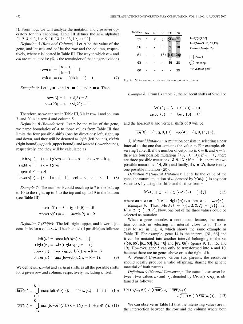
Fig. 4. Mutation and crossover for continuous attributes.
Example 8: From Example 7, the adjacent shifts of 9 will be
and the horizontal and vertical shifts of 9 will be
3) Natural Mutation: A mutation consists in selecting a nearinterval to the one that contains the value . For example, ob-serving Table III, if the number of cutpoints is k , and ,there are four possible mutations ; if , thereare three possible mutations ; if , there are twopossible mutations ; and finally, if , there is onlyone possible mutation .
Definition 8 (Natural Mutation): Let be the value of thegene, the natural mutation of , denoted by , is any nearvalue to by using the shifts and distinct from
(12)
where .Example 9: Thus, , i.e.,
. Now, one out of the three values could beselected as mutation.
When a gene encodes a continuous feature, the muta-tion consists in selecting an interval close to it. This iseasy to see in Fig. 4, which shows the same example asTable III. For example, gene 14 is the interval [61, 66] andit can be mutated into another interval belonging to the set
and (genes 9, 13, 15, and19). However, gene 5 can only be transformed into 4 and 10,because there are no genes above or to the right of it.
4) Natural Crossover: Given two parents, the crossovershould ideally produce a valid offspring, sharing the geneticmaterial of both parents.
Definition 9 (Natural Crossover): The natural crossover be-tween two values and , denoted by is ob-tained as follows:
(13)
We can observe in Table III that the interesting values are inthe intersection between the row and the column where both
AGUILAR-RUIZ et al.: NATURAL ENCODING FOR EVOLUTIONARY SUPERVISED LEARNING 473
values being crossed are placed. Only when the values andare located in the same row or column, the interval will be
inside the other.Example 10: Thus
The general case of crossover between two parents is illustratedin Fig. 4. The possible offspring is formed by those numbersin the intersection between the row and the column of both par-ents. For example, the crossover between genes 5 and 14 (withinsquares) generates as offspring genes 4 and 15 (within circles).In Table III, we can see that this offspring makes sense becauseit uses every boundary from the parents.
V. ALGORITHM
HIDER is a tool that produces a hierarchical set of rules [22].When a new example is to be classified, the set of rules is se-quentially evaluated according to the hierarchy. If the exampledoes not fulfil a rule, the next one in the hierarchy order is eval-uated. This process is repeated until the example matches everycondition of a rule and it is classified with the class that suchrule establishes.
HIDER uses an EA to search for the best solutions. Since theaim is to obtain a set of decision rules, the population of the EAis formed by some possible solutions. Each genetic individual isa rule that evolves applying the mutation and crossover opera-tors. In each generation, some individuals are selected accordingto their goodness and they are included in the next populationalong with their offspring.
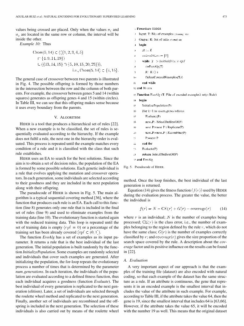
The pseudocode of HIDER is shown in Fig. 5. The main al-gorithm is a typical sequential covering method [36], where thefunction that produces each rule is an EA. Each call to this func-tion (line 8) generates only one rule that is included in the finalset of rules (line 9) and used to eliminate examples from thetraining data (line 10). The evolutionary function is started againwith the reduced training data. This loop is repeated until theset of training data is empty or a percentage of thetraining set has been already covered .
The function EvoAlg has a set of examples as its input pa-rameter. It returns a rule that is the best individual of the lastgeneration. The initial population is built randomly by the func-tion InitializePopulation. Some examples are randomly selectedand individuals that cover such examples are generated. Afterinitializing the population, the for-loop repeats the evolutionaryprocess a number of times that is determined by the parameternum generations. In each iteration, the individuals of the popu-lation are evaluated according to a defined fitness function, thuseach individual acquires a goodness (function Evaluate). Thebest individual of every generation is replicated to the next gen-eration (elitism). Later, a set of individuals are selected throughthe roulette wheel method and replicated to the next generation.Finally, another set of individuals are recombined and the off-spring is included in the next generation. The selection of theseindividuals is also carried out by means of the roulette wheel
Fig. 5. Pseudocode of HIDER.
method. Once the loop finishes, the best individual of the lastgeneration is returned.
Equation (14) gives the fitness function used by HIDER
during the evaluation process. The greater the value, the betterthe individual is
(14)
where is an individual; is the number of examples beingprocessed; is the class error, i.e., the number of exam-ples belonging to the region defined by the rule , which do nothave the same class; is the number of examples correctlyclassified by ; and gives the size proportion of thesearch space covered by the rule. A description about the cov-erage factor and its positive influence on the results can be foundin [22].
A. Evaluation
A very important aspect of our approach is that the exam-ples of the training file (dataset) are also encoded with naturalcoding, so that each example of the dataset has the same struc-ture as a rule. If an attribute is continuous, the gene that repre-sents it in an encoded example is the smallest interval that in-cludes the value of the attribute in such example. For example,according to Table III, if the attribute takes the value 64, then thegene is 19, since the smallest interval that includes 64 is [63,66].However, if the attribute takes the value 65, it will be encodedwith the number 19 as well. This means that the original dataset
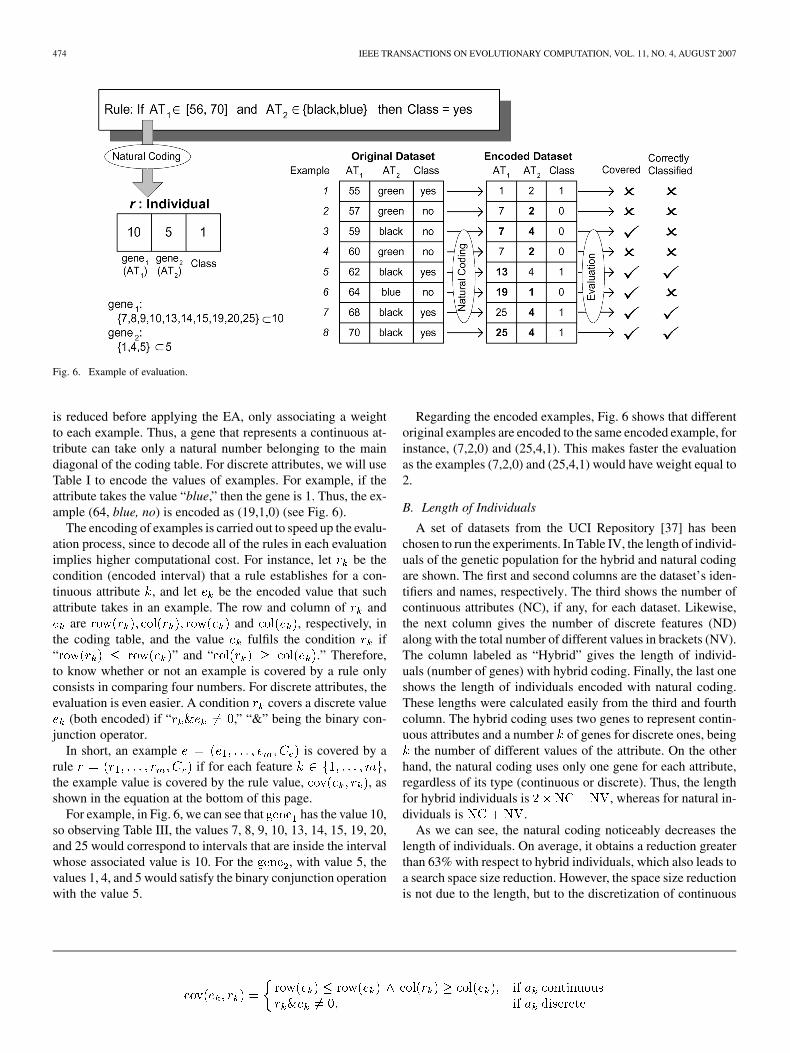
474 IEEE TRANSACTIONS ON EVOLUTIONARY COMPUTATION, VOL. 11, NO. 4, AUGUST 2007
Fig. 6. Example of evaluation.
is reduced before applying the EA, only associating a weightto each example. Thus, a gene that represents a continuous at-tribute can take only a natural number belonging to the maindiagonal of the coding table. For discrete attributes, we will useTable I to encode the values of examples. For example, if theattribute takes the value “blue,” then the gene is 1. Thus, the ex-ample (64, blue, no) is encoded as (19,1,0) (see Fig. 6).
The encoding of examples is carried out to speed up the evalu-ation process, since to decode all of the rules in each evaluationimplies higher computational cost. For instance, let be thecondition (encoded interval) that a rule establishes for a con-tinuous attribute , and let be the encoded value that suchattribute takes in an example. The row and column of and
are and , respectively, inthe coding table, and the value fulfils the condition if“ ” and “ .” Therefore,to know whether or not an example is covered by a rule onlyconsists in comparing four numbers. For discrete attributes, theevaluation is even easier. A condition covers a discrete value
(both encoded) if “ ,” “&” being the binary con-junction operator.
In short, an example is covered by arule if for each feature ,the example value is covered by the rule value, , asshown in the equation at the bottom of this page.
For example, in Fig. 6, we can see that has the value 10,so observing Table III, the values 7, 8, 9, 10, 13, 14, 15, 19, 20,and 25 would correspond to intervals that are inside the intervalwhose associated value is 10. For the , with value 5, thevalues 1, 4, and 5 would satisfy the binary conjunction operationwith the value 5.
Regarding the encoded examples, Fig. 6 shows that differentoriginal examples are encoded to the same encoded example, forinstance, (7,2,0) and (25,4,1). This makes faster the evaluationas the examples (7,2,0) and (25,4,1) would have weight equal to2.
B. Length of Individuals
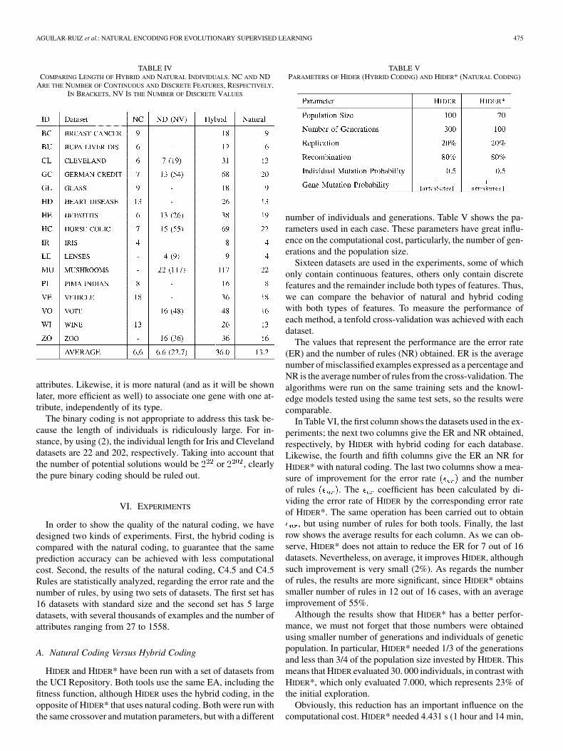
A set of datasets from the UCI Repository [37] has beenchosen to run the experiments. In Table IV, the length of individ-uals of the genetic population for the hybrid and natural codingare shown. The first and second columns are the dataset’s iden-tifiers and names, respectively. The third shows the number ofcontinuous attributes (NC), if any, for each dataset. Likewise,the next column gives the number of discrete features (ND)along with the total number of different values in brackets (NV).The column labeled as “Hybrid” gives the length of individ-uals (number of genes) with hybrid coding. Finally, the last oneshows the length of individuals encoded with natural coding.These lengths were calculated easily from the third and fourthcolumn. The hybrid coding uses two genes to represent contin-uous attributes and a number of genes for discrete ones, being
the number of different values of the attribute. On the otherhand, the natural coding uses only one gene for each attribute,regardless of its type (continuous or discrete). Thus, the lengthfor hybrid individuals is , whereas for natural in-dividuals is .
As we can see, the natural coding noticeably decreases thelength of individuals. On average, it obtains a reduction greaterthan 63% with respect to hybrid individuals, which also leads toa search space size reduction. However, the space size reductionis not due to the length, but to the discretization of continuous
AGUILAR-RUIZ et al.: NATURAL ENCODING FOR EVOLUTIONARY SUPERVISED LEARNING 475
TABLE IVCOMPARING LENGTH OF HYBRID AND NATURAL INDIVIDUALS. NC AND ND
ARE THE NUMBER OF CONTINUOUS AND DISCRETE FEATURES, RESPECTIVELY.IN BRACKETS, NV IS THE NUMBER OF DISCRETE VALUES
attributes. Likewise, it is more natural (and as it will be shownlater, more efficient as well) to associate one gene with one at-tribute, independently of its type.
The binary coding is not appropriate to address this task be-cause the length of individuals is ridiculously large. For in-stance, by using (2), the individual length for Iris and Clevelanddatasets are 22 and 202, respectively. Taking into account thatthe number of potential solutions would be or , clearlythe pure binary coding should be ruled out.
VI. EXPERIMENTS
In order to show the quality of the natural coding, we havedesigned two kinds of experiments. First, the hybrid coding iscompared with the natural coding, to guarantee that the sameprediction accuracy can be achieved with less computationalcost. Second, the results of the natural coding, C4.5 and C4.5Rules are statistically analyzed, regarding the error rate and thenumber of rules, by using two sets of datasets. The first set has16 datasets with standard size and the second set has 5 largedatasets, with several thousands of examples and the number ofattributes ranging from 27 to 1558.
A. Natural Coding Versus Hybrid Coding
HIDER and HIDER* have been run with a set of datasets fromthe UCI Repository. Both tools use the same EA, including thefitness function, although HIDER uses the hybrid coding, in theopposite of HIDER* that uses natural coding. Both were run withthe same crossover and mutation parameters, but with a different
TABLE VPARAMETERS OF HIDER (HYBRID CODING) AND HIDER* (NATURAL CODING)
number of individuals and generations. Table V shows the pa-rameters used in each case. These parameters have great influ-ence on the computational cost, particularly, the number of gen-erations and the population size.
Sixteen datasets are used in the experiments, some of whichonly contain continuous features, others only contain discretefeatures and the remainder include both types of features. Thus,we can compare the behavior of natural and hybrid codingwith both types of features. To measure the performance ofeach method, a tenfold cross-validation was achieved with eachdataset.
The values that represent the performance are the error rate(ER) and the number of rules (NR) obtained. ER is the averagenumber of misclassified examples expressed as a percentage andNR is the average number of rules from the cross-validation. Thealgorithms were run on the same training sets and the knowl-edge models tested using the same test sets, so the results werecomparable.
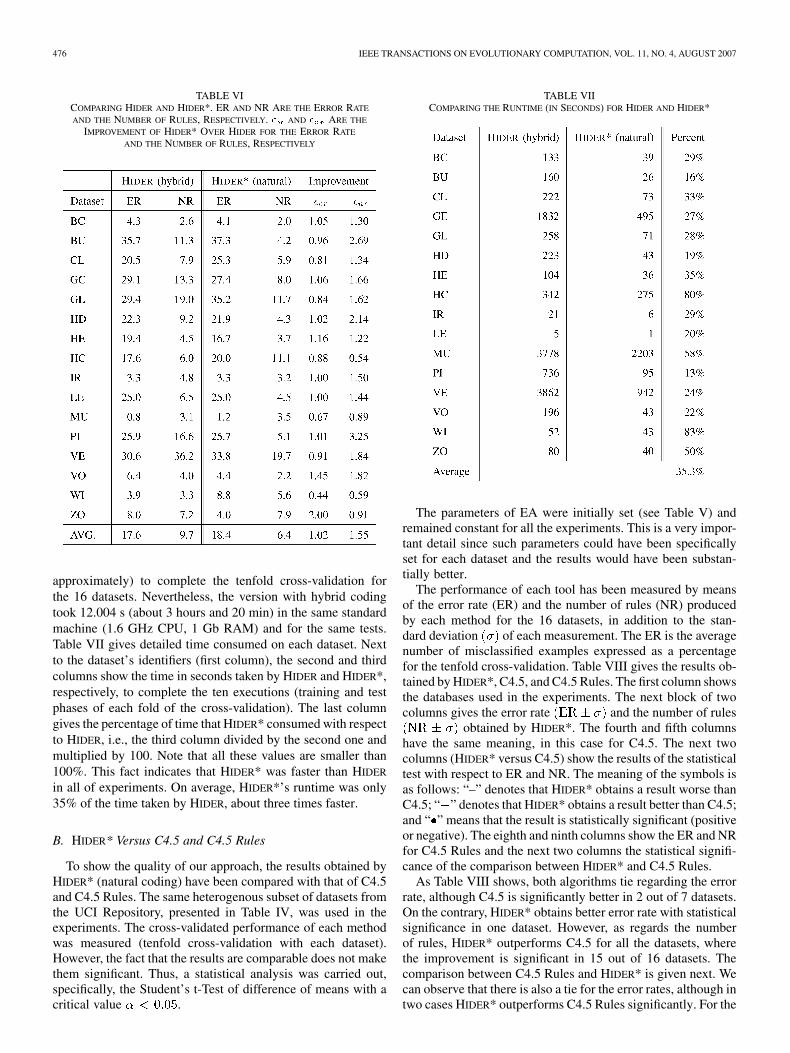
In Table VI, the first column shows the datasets used in the ex-periments; the next two columns give the ER and NR obtained,respectively, by HIDER with hybrid coding for each database.Likewise, the fourth and fifth columns give the ER an NR forHIDER* with natural coding. The last two columns show a mea-sure of improvement for the error rate and the numberof rules . The coefficient has been calculated by di-viding the error rate of HIDER by the corresponding error rateof HIDER*. The same operation has been carried out to obtain
, but using number of rules for both tools. Finally, the lastrow shows the average results for each column. As we can ob-serve, HIDER* does not attain to reduce the ER for 7 out of 16datasets. Nevertheless, on average, it improves HIDER, althoughsuch improvement is very small (2%). As regards the numberof rules, the results are more significant, since HIDER* obtainssmaller number of rules in 12 out of 16 cases, with an averageimprovement of 55%.
Although the results show that HIDER* has a better perfor-mance, we must not forget that those numbers were obtainedusing smaller number of generations and individuals of geneticpopulation. In particular, HIDER* needed 1/3 of the generationsand less than 3/4 of the population size invested by HIDER. Thismeans that HIDER evaluated 30. 000 individuals, in contrast withHIDER*, which only evaluated 7.000, which represents 23% ofthe initial exploration.
Obviously, this reduction has an important influence on thecomputational cost. HIDER* needed 4.431 s (1 hour and 14 min,
476 IEEE TRANSACTIONS ON EVOLUTIONARY COMPUTATION, VOL. 11, NO. 4, AUGUST 2007
TABLE VICOMPARING HIDER AND HIDER*. ER AND NR ARE THE ERROR RATE
AND THE NUMBER OF RULES, RESPECTIVELY. � AND � ARE THE
IMPROVEMENT OF HIDER* OVER HIDER FOR THE ERROR RATE
AND THE NUMBER OF RULES, RESPECTIVELY
approximately) to complete the tenfold cross-validation forthe 16 datasets. Nevertheless, the version with hybrid codingtook 12.004 s (about 3 hours and 20 min) in the same standardmachine (1.6 GHz CPU, 1 Gb RAM) and for the same tests.Table VII gives detailed time consumed on each dataset. Nextto the dataset’s identifiers (first column), the second and thirdcolumns show the time in seconds taken by HIDER and HIDER*,respectively, to complete the ten executions (training and testphases of each fold of the cross-validation). The last columngives the percentage of time that HIDER* consumed with respectto HIDER, i.e., the third column divided by the second one andmultiplied by 100. Note that all these values are smaller than100%. This fact indicates that HIDER* was faster than HIDER
in all of experiments. On average, HIDER*’s runtime was only35% of the time taken by HIDER, about three times faster.
B. HIDER* Versus C4.5 and C4.5 Rules
To show the quality of our approach, the results obtained byHIDER* (natural coding) have been compared with that of C4.5and C4.5 Rules. The same heterogenous subset of datasets fromthe UCI Repository, presented in Table IV, was used in theexperiments. The cross-validated performance of each methodwas measured (tenfold cross-validation with each dataset).However, the fact that the results are comparable does not makethem significant. Thus, a statistical analysis was carried out,specifically, the Student’s t-Test of difference of means with acritical value .
TABLE VIICOMPARING THE RUNTIME (IN SECONDS) FOR HIDER AND HIDER*
The parameters of EA were initially set (see Table V) andremained constant for all the experiments. This is a very impor-tant detail since such parameters could have been specificallyset for each dataset and the results would have been substan-tially better.
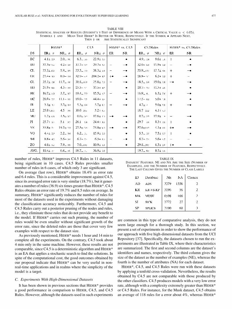
The performance of each tool has been measured by meansof the error rate (ER) and the number of rules (NR) producedby each method for the 16 datasets, in addition to the stan-dard deviation of each measurement. The ER is the averagenumber of misclassified examples expressed as a percentagefor the tenfold cross-validation. Table VIII gives the results ob-tained by HIDER*, C4.5, and C4.5 Rules. The first column showsthe databases used in the experiments. The next block of twocolumns gives the error rate and the number of rules
obtained by HIDER*. The fourth and fifth columnshave the same meaning, in this case for C4.5. The next twocolumns (HIDER* versus C4.5) show the results of the statisticaltest with respect to ER and NR. The meaning of the symbols isas follows: “–” denotes that HIDER* obtains a result worse thanC4.5; “ ” denotes that HIDER* obtains a result better than C4.5;and “ ” means that the result is statistically significant (positiveor negative). The eighth and ninth columns show the ER and NRfor C4.5 Rules and the next two columns the statistical signifi-cance of the comparison between HIDER* and C4.5 Rules.
As Table VIII shows, both algorithms tie regarding the errorrate, although C4.5 is significantly better in 2 out of 7 datasets.On the contrary, HIDER* obtains better error rate with statisticalsignificance in one dataset. However, as regards the numberof rules, HIDER* outperforms C4.5 for all the datasets, wherethe improvement is significant in 15 out of 16 datasets. Thecomparison between C4.5 Rules and HIDER* is given next. Wecan observe that there is also a tie for the error rates, although intwo cases HIDER* outperforms C4.5 Rules significantly. For the
AGUILAR-RUIZ et al.: NATURAL ENCODING FOR EVOLUTIONARY SUPERVISED LEARNING 477
TABLE VIIISTATISTICAL ANALYSIS OF RESULTS (STUDENT’S T-TEST OF DIFFERENCE OF MEANS WITH A CRITICAL VALUE � < 0:05).
SYMBOLS + AND � MEAN THAT HIDER* IS BETTER OR WORSE, RESPECTIVELY. IF THE SYMBOL � APPEARS NEXT,THEN + OR � ARE STATISTICALLY SIGNIFICANT
number of rules, HIDER* improves C4.5 Rules in 11 datasets,being significant in 10 cases. C4.5 Rules provides smallernumber of rules in 6 cases, of which only 3 are significant.
On average (last row), HIDER* obtains 18.4% as error rateand 6.4 rules. This is a considerable improvement against C4.5,since its averaged error rate is very similar (18.7%), but it gener-ates a number of rules (36.9) six times greater than HIDER*. C4.5Rules obtains an error rate of 19.7% and 8.5 rules on average. Insummary, HIDER* significantly reduces the number of rules formost of the datasets used in the experiments without damagingthe classification accuracy noticeably. Furthermore, C4.5 andC4.5 Rules carry out a posterior pruning of the nodes and rules,i.e., they eliminate those rules that do not provide any benefit tothe model. If HIDER* carries out such pruning, the number ofrules would be even smaller without significant growth of theerror rate, since the deleted rules are those that cover very fewexamples with respect to the dataset size.
As previously mentioned, HIDER* needs 1 hour and 14 min tocomplete all the experiments. On the contrary, C4.5 took about4 min only in the same machine. However, these results are notcomparable, since C4.5 is a deterministic algorithm and HIDER*is an EA that applies a stochastic search to find the solutions. Inspite of the computational cost, the good outcomes obtained byour proposal indicate that HIDER* can be very useful in non-real-time applications and in realms where the simplicity of themodel is a target.
C. Experiments With High-Dimensional Datasets
It has been shown in previous sections that HIDER* providesa good performance in comparison to HIDER, C4.5, and C4.5Rules. However, although the datasets used in such experiments
TABLE IXDATASETS’ FEATURES. NE AND NA ARE THE SIZE (NUMBER OF
EXAMPLES), AND THE NUMBER OF FEATURES, RESPECTIVELY.THE LAST COLUMN GIVES THE NUMBER OF CLASS LABELS
are common in this type of comparative analysis, they do notseem large enough for a thorough study. In this section, wepresent a set of experiments in order to show the performance ofour approach with five high-dimensional datasets from the UCIRepository [37]. Specifically, the datasets chosen to run the ex-periments are illustrated in Table IX, where their characteristicsare summarized. The first and second columns are the dataset’sidentifiers and names, respectively. The third column gives thesize of the dataset as the number of examples (NE), whereas thefourth is the number of attributes (NA) for each dataset.
HIDER*, C4.5, and C4.5 Rules were run with these datasetsby applying a tenfold cross-validation. Nevertheless, the resultsobtained by C4.5 are not comparable with those produced bythe other classifiers. C4.5 produces models with a very low errorrate, although with a complexity extremely greater than HIDER*or C4.5 Rules. For instance, for the Musk dataset, C4.5 obtainsan average of 118 rules for a error about 4%, whereas HIDER*
478 IEEE TRANSACTIONS ON EVOLUTIONARY COMPUTATION, VOL. 11, NO. 4, AUGUST 2007
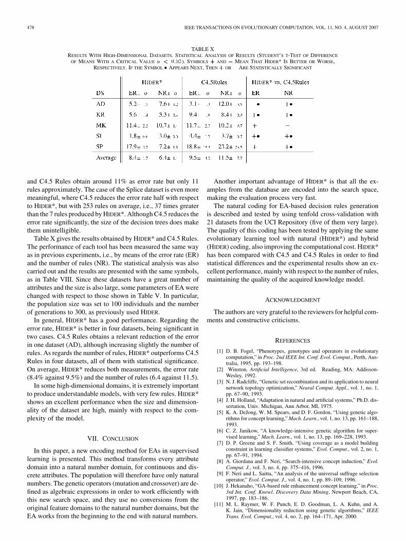
TABLE XRESULTS WITH HIGH-DIMENSIONAL DATASETS. STATISTICAL ANALYSIS OF RESULTS (STUDENT’S T-TEST OF DIFFERENCE
OF MEANS WITH A CRITICAL VALUE � < 0:05). SYMBOLS + AND � MEAN THAT HIDER* IS BETTER OR WORSE,RESPECTIVELY. IF THE SYMBOL � APPEARS NEXT, THEN + OR � ARE STATISTICALLY SIGNIFICANT
and C4.5 Rules obtain around 11% as error rate but only 11rules approximately. The case of the Splice dataset is even moremeaningful, where C4.5 reduces the error rate half with respectto HIDER*, but with 253 rules on average, i.e., 37 times greaterthan the 7 rules produced by HIDER*. Although C4.5 reduces theerror rate significantly, the size of the decision trees does makethem unintelligible.
Table X gives the results obtained by HIDER* and C4.5 Rules.The performance of each tool has been measured the same wayas in previous experiments, i.e., by means of the error rate (ER)and the number of rules (NR). The statistical analysis was alsocarried out and the results are presented with the same symbols,as in Table VIII. Since these datasets have a great number ofattributes and the size is also large, some parameters of EA werechanged with respect to those shown in Table V. In particular,the population size was set to 100 individuals and the numberof generations to 300, as previously used HIDER.
In general, HIDER* has a good performance. Regarding theerror rate, HIDER* is better in four datasets, being significant intwo cases. C4.5 Rules obtains a relevant reduction of the errorin one dataset (AD), although increasing slightly the number ofrules. As regards the number of rules, HIDER* outperforms C4.5Rules in four datasets, all of them with statistical significance.On average, HIDER* reduces both measurements, the error rate(8.4% against 9.5%) and the number of rules (6.4 against 11.5).
In some high-dimensional domains, it is extremely importantto produce understandable models, with very few rules. HIDER*shows an excellent performance when the size and dimension-ality of the dataset are high, mainly with respect to the com-plexity of the model.
VII. CONCLUSION
In this paper, a new encoding method for EAs in supervisedlearning is presented. This method transforms every attributedomain into a natural number domain, for continuous and dis-crete attributes. The population will therefore have only naturalnumbers. The genetic operators (mutation and crossover) are de-fined as algebraic expressions in order to work efficiently withthis new search space, and they use no conversions from theoriginal feature domains to the natural number domains, but theEA works from the beginning to the end with natural numbers.
Another important advantage of HIDER* is that all the ex-amples from the database are encoded into the search space,making the evaluation process very fast.
The natural coding for EA-based decision rules generationis described and tested by using tenfold cross-validation with21 datasets from the UCI Repository (five of them very large).The quality of this coding has been tested by applying the sameevolutionary learning tool with natural (HIDER*) and hybrid(HIDER) coding, also improving the computational cost. HIDER*has been compared with C4.5 and C4.5 Rules in order to findstatistical differences and the experimental results show an ex-cellent performance, mainly with respect to the number of rules,maintaining the quality of the acquired knowledge model.
ACKNOWLEDGMENT
The authors are very grateful to the reviewers for helpful com-ments and constructive criticisms.
REFERENCES
[1] D. B. Fogel, “Phenotypes, genotypes and operators in evolutionarycomputation,” in Proc. 2nd IEEE Int. Conf. Evol. Comput., Perth, Aus-tralia, 1995, pp. 193–198.
[2] Winston, Artificial Intelligence, 3rd ed. Reading, MA: Addisson-Wesley, 1992.
[3] N. J. Radcliffe, “Genetic set recombination and its application to neuralnetwork topology optimization,” Neural Comput. Appl., vol. 1, no. 1,pp. 67–90, 1993.
[4] J. H. Holland, “Adaptation in natural and artificial systems,” Ph.D. dis-sertation, Univ. Michigan, Ann Arbor, MI, 1975.
[5] K. A. DeJong, W. M. Spears, and D. F. Gordon, “Using genetic algo-rithms for concept learning,” Mach. Learn., vol. 1, no. 13, pp. 161–188,1993.
[6] C. Z. Janikow, “A knowledge-intensive genetic algorithm for super-vised learning,” Mach. Learn., vol. 1, no. 13, pp. 169–228, 1993.
[7] D. P. Greene and S. F. Smith, “Using coverage as a model buildingconstraint in learning classifier systems,” Evol. Comput., vol. 2, no. 1,pp. 67–91, 1994.
[8] A. Giordana and F. Neri, “Search-intensive concept induction,” Evol.Comput. J., vol. 3, no. 4, pp. 375–416, 1996.
[9] F. Neri and L. Saitta, “An analysis of the universal suffrage selectionoperator,” Evol. Comput. J., vol. 4, no. 1, pp. 89–109, 1996.
[10] J. Hekanaho, “GA-based rule enhancement concept learning,” in Proc.3rd Int. Conf. Knowl. Discovery Data Mining, Newport Beach, CA,1997, pp. 183–186.
[11] M. L. Raymer, W. F. Punch, E. D. Goodman, L. A. Kuhn, and A.K. Jain, “Dimensionality reduction using genetic algorithms,” IEEETrans. Evol. Comput., vol. 4, no. 2, pp. 164–171, Apr. 2000.
AGUILAR-RUIZ et al.: NATURAL ENCODING FOR EVOLUTIONARY SUPERVISED LEARNING 479
[12] J. R. Cano, F. Herrera, and M. Lozano, “Using evolutionary algorithmsas instance selection for data reduction in KDD: An experimentalstudy,” IEEE Trans. Evol. Comput., vol. 7, no. 6, pp. 561–575, Dec.2003.
[13] R. Caruana and J. D. Schaffer, “Representation and hidden bias: Grayversus binary codign for genetic algorithms,” in Proc. Int. Conf. Mach.Learn., 1988, pp. 153–161.
[14] R. Caruana, J. D. Schaffer, and L. J. Eshelman, “Using multiple rep-resentations to improve inductive bias: Gray and binary coding for ge-netic algorithms,” in Proc. Int. Conf. Mach. Learn., 1989, pp. 375–378.
[15] U. K. Chakraborty and C. Z. Janikow, “An analysis of gray versus bi-nary encoding in genetic search,” Inf. Sci., no. 156, pp. 253–269, 2003.
[16] F. Rothlauf and D. Goldberg, “Prufer numbers and genetic algorithms,”PPSN, pp. 395–404, 2000.
[17] J. A. Lozano and P. Larrañaga, “Applying genetic algorithms to searchfor the best hierarchical clustering of a dataset,” Pattern Recogn. Lett.,vol. 20, no. 9, pp. 911–918, 1999.
[18] F. Herrera, M. Lozano, and J. L. Verdegay, “Tackling real-coded ge-netic algorithms: Operators and tools for the behavior analysis,” Arti.Intell. Rev., vol. 12, pp. 265–319, 1998.
[19] L. J. Eshelman and J. D. Schaffer, “Real-coded genetic algorithmsand interval-schemata,” Foundations of Genetic Algorithms-2, pp.187–202, 1993.
[20] K. Deb and A. Kumar, “Real-coded genetic algorithms with simulatedbinary crossover: Studies on multimodal and multiobjective problems,”Complex Syst., vol. 9, pp. 431–454, 1995.
[21] G. Venturini, “SIA: A supervised inductive algorithm with geneticsearch for learning attributes based concepts,” in Proc. Eur. Conf.Mach. Learn., 1993, pp. 281–296.
[22] J. S. Aguilar-Ruiz, J. C. Riquelme, and M. Toro, “Evolutionary learningof hierarchical decision rules,” IEEE Trans. Syst., Man, Cybern., PartB, vol. 33, no. 2, pp. 324–331, 2003.
[23] S. K. Sharma and G. W. Irwing, “Fuzzy coding of genetic algorithms,”IEEE Trans. Evol. Comput., vol. 7, no. 4, pp. 344–355, Aug. 2003.
[24] P. P. Bonissone, R. Subbu, N. Eklund, and T. R. Kiehl, “Evolutionaryalgorithms + domain knowledge = real-world evolutionary compu-tation,” IEEE Trans. Evol. Comput., vol. 10, no. 3, pp. 256–280, Jun.2006.
[25] J. R. Quinlan, C4.5: Programs for Machine Learning. San Mateo,CA: Morgan Kaufmann, 1993.
[26] D. Dougherty, R. Kohavi, and M. Sahami, “Supervised and unsuper-vised discretization of continuous features,” in Proc. 12th Int. Conf.Mach. Learn., 1995, pp. 194–202.
[27] J. S. Aguilar-Ruiz, J. Bacardit, and F. Divina, “Experimental evalua-tion of discretization schemes for rule induction,” in Genetic and Evo-lutionary Computation, ser. Lecture Notes in Computer Science.Berlin, Germany: Springer-Verlag, Jun. 2004, pp. 828–839.
[28] R. C. Holte, “Very simple classification rules perform well on mostcommonly used datasets,” Mach. Learn., vol. 11, pp. 63–91, 1993.
[29] U. M. Fayyad and K. B. Irani, “Multi-interval discretization of con-tinuous valued attributes for classification learning,” in Proc. 13th Int.Joint Conf. Artif. Intell., 1993, pp. 1022–1027.
[30] R. Giráldez, J. S. Aguilar-Ruiz, and J. C. Riquelme, “Discretization ori-ented to decision rules generation,” in Knowledge-Based Intelligent In-formation Engineering Systems & Allied Technologies. Amsterdam,The Netherlands: IOS-Press, 2002, pp. 275–279.
[31] J. Antonisse, “A new interpretation of schema notation that overturnsthe binary encoding constraint,” in Proc. 3rd Int. Conf. Genetic Algo-rithms, 1989, pp. 86–97.
[32] S. Bhattacharyya and G. J. Koehler, “An analysis of non-binary geneticalgorithms with cardinality 2 ,” Complex Syst., vol. 8, pp. 227–256,1994.
[33] G. J. Koehler, S. Bhattacharyya, and M. D. Vose, “General cardinalitygenetic algorithms,” Evol. Comput., vol. 5, no. 4, pp. 439–459, 1998.
[34] M. D. Vose and A. H. Wright, “The simple genetic algorithm and theWalsh transform: Part I, Theory,” Evol. Comput., vol. 6, no. 3, pp.253–273, 1998.
[35] M. D. Vose and A. H. Wright, “The simple genetic algorithm and theWalsh transform: Part II, The inverse,” Evol. Comput., vol. 6, no. 3, pp.275–289, 1998.
[36] T. Mitchell, Machine Learning. New York: McGraw-Hill, 1997.[37] C. Blake and E. K. Merz, “UCI repository of machine learning
databases,” Univ. California, Irvine, CA, 1998.
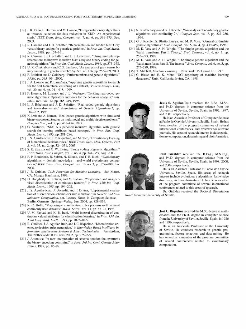
Jesús S. Aguilar-Ruiz received the B.Sc., M.Sc.,and Ph.D. degrees in computer science from theUniversity of Seville, Seville, Spain, in 1992, 1997,and 2001, respectively.
He is an Associate Professor of Computer Scienceat Pablo de Olavide University, Seville, Spain. He hasbeen member of the program committee of severalinternational conferences, and reviewer for relevantjournals. His areas of research interest include evolu-tionary computation, data mining and bioinformatics.
Raúl Giráldez received the B.Eng., M.S.Eng.,and Ph.D. degrees in computer science from theUniversity of Seville, Seville, Spain, in 1998, 2000,and 2004, respectively.
He is an Assistant Professor at Pablo de OlavideUniversity, Seville, Spain. His areas of researchinterest include evolutionary algorithms, knowledgediscovery, and bioinformatics. He has been memberof the program committee of several internationalconferences related to this areas of research.
Dr. Giráldez received the Doctoral DissertationAward from the University of Seville.
José C. Riquelme received the M.Sc. degree in math-ematics and the Ph.D. degree in computer sciencefrom the University of Seville, Seville, Spain, in 1986and 1996, respectively.
He is an Associate Professor at the Universityof Seville. He conducts research in genetic pro-gramming, feature selection, and data mining. Hehas served as a member of the program committeeof several conferences related to evolutionarycomputation.