evolutionary computation in bioinformatics
TRANSCRIPT

1
Tutorial on Evolutionary Computation in Bioinformatics: Part I
Gary B. FogelVice PresidentNatural Selection, Inc.9330 Scranton Rd., Suite 150San Diego, CA 92121 USA
2007 IEEE Congress on Evolutionary Computation 2007 IEEE Congress on Evolutionary Computation -- September 25, 2007 September 25, 2007 -- SingaporeSingapore
Kay C. WieseSchool of Computing ScienceSimon Fraser UniversityCanadaChair: IEEE CIS Bioinformatics and Bioengineering Technical Committee

2
Bioinformatics - DefinitionBioinformatics
The field of science in which biology, computer science, and information technology merge to form a single discipline. The ultimate goal of the field is to enable the discovery of new biological insights as well as to create a global perspective from which unifying principles in biology can be discerned. Classically: storage and information retrieval of biological data
Computational BiologyUse of computers to analyze and interpret biological data Typically nucleotide, RNA, protein sequences, structures
Largely interchangeable in the literatureNew tools for data access and managementNew algorithms and statistics for pattern identification and prediction

3
Bioinformatics - HistoryRevolutionary methods in molecular biology
DNA sequencingProtein structure determinationDrug design and development
Exponential growth of biological informationComputational requirement for
Database storage of informationOrganization of informationTools for analysis of data
The transition of biology from “wet-lab” to “dry-lab/information science”

4
Bioinformatics / Computational Biology
The use of techniques from applied mathematics, informatics, statistics, and computer science to solve (typically noisy) biological problems
Multiple sequence alignmentIdentification of functional regions or motifsClassification of dataPhylogenetic analysisMolecular structure determination and foldingGeneticsDiagnostics and medical applications

5
Why is bioinformatics important?
Modeling via bioinformatics may provide answers to questions related to human health and evolutionDevelopment of small molecule drugs to combat infection and diseaseDiagnosis and prognosis, leading to more effective medicine

6http://www.ncbi.nlm.nih.gov/Genbank/index.html

7
Bioinformatics

8
DNA RNA ProteinTranscription Translation
←→ →Reverse transcription
Information Function
Information Flow in the Cell

9
A More Modern View…

10
What is DNA?Adenine (A)Thymine (T)Guanine (G) Cytosine (C)
A – TG – C

11
Exons (coding regions)
Introns (non-coding regions)Promoter
Enhancer
DNA
Enhancers and promoters affect the level of transcription and act as on-off switches (potentiometers)
Gene Organization

12
Promoter DataReese' promoters dataset:http://www.fruitfly.org/seq_tools/datasets/Human/promoter/ Results for NNPP on promoters taken from the Eukaryotic PromoterDatabase, EPD and genes GenBank database. 300 promoter sequences of 51 bp each. (40bp upstream and 11 bp downstream from the known transcription start site)3,000 non-promoter regions, also each of 51 bp, some from coding regions and some introns. TSS
40 bp 11 bp

13

14
RNA
Adenine (A)Uracil (U)Guanine (G) Cytosine (C)
A – UG – CG – U

15
>100 Gigabases of Information
Over 100 Gigabases of DNA and RNA sequence information in GenBank, EMBL, and DDBJ as of 2005
(roughly the same order of magnitude as the number of nerve cells in a human brain)individual genes partial and complete genomes over 165,000 organismsFree access
http://www.nlm.nih.gov/news/press_releases/dna_rna_100_gig.html

16
Databases
GenBankNational Institutes of Health65 gigabases of sequence information
EMBLEuropean Molecular Biology Laboratory
DDBJDNA DataBank of Japan

17
Microarrays
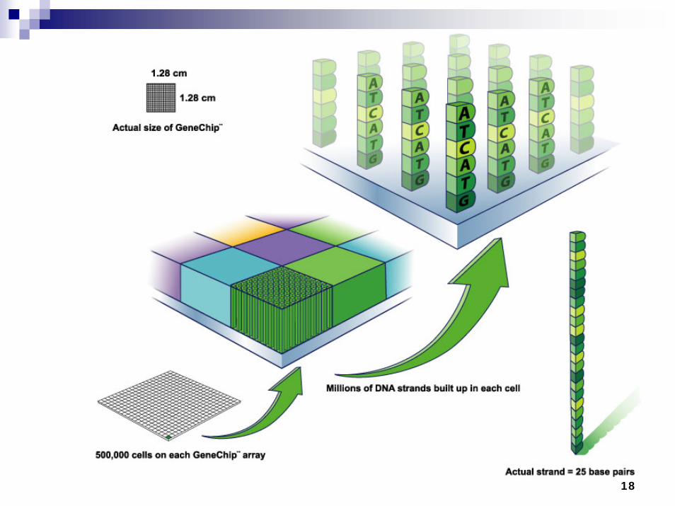
18

19

20

21
diauxic shift timecourse: 20.5 hrdiauxic shift timecourse: 0 hr
DeRisi JL, et al. (1997) Science 278(5338):680-6

22

23
Microarray DatabasesStanford Microarray Database
Experiments : 66571 Public Experiments : 12596 Spots : 1983883115 Users : 1633 Labs : 319 Organisms : 50 Publications : 350
http://genome-www5.stanford.edu/statistics.html

24

25
GGUGCGCGUUAU
GARY
26
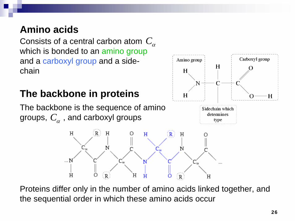
Amino acids
The backbone in proteins
Consists of a central carbon atom which is bonded to an amino groupand a carboxyl group and a side-chain
αCThe backbone is the sequence of amino groups, , and carboxyl groups
αC
Proteins differ only in the number of amino acids linked together, and the sequential order in which these amino acids occur

27
Protein
20 amino acid typesFolding
28
Protein Analysis
Broad area of bioinformatics includes:SequenceStructureFunction
Focus today on:Finding MotifsClassificationPrediction

29
Primary Data Sources
Sequence – pdb, swissProtStructure – cath, dsspFunction - cath, scopExperimentally derived from a lab or group of labs (e.g. NMR data for membrane spanning proteins)

30
Quantitative Structure-Activity Relationships
Molecule/activity set10s-100s of features = (hydrophobicity, electronic effects, steric effects, etc.)Training / testing / validation setsReduce the number of featuresPredictive model for future compound discoveryBetter understanding of true biological mechanism of action

31
Phylogenetics
Determining the history of life on Earth using sequence information or other characteristics/featuresDevelop a tree-like representation Factorial increase in the number of possible trees as the number of sequences/features increasesBetter search algorithms for the space of tree representations for resolution of a “true” tree

32

33
Data Pitfalls
Bias due to homologyDirty data due to unknownsNot enough examples to train fromOutliersOut of dateGarbage in, garbage out

34
Predictors and Classifiers
Predictors – given an unknown data sample provide a measure of confidence that it belongs to the set the model was constructed to representClassifiers – given a set of heterogeneous data separate the data into classes.
Supervised – trained on a set of known examplesUnsupervised – number of classes is not known in advance (also referred to as clustering)

35
Clustering
Clustering is the classification of similar objects into different groups
More precisely - the partitioning of a data set into subsets (clusters), so that the data in each subset (ideally) share some common trait - often proximity according to some defined distance measure.
36
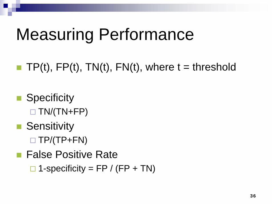
Measuring Performance
TP(t), FP(t), TN(t), FN(t), where t = threshold
SpecificityTN/(TN+FP)
SensitivityTP/(TP+FN)
False Positive Rate1-specificity = FP / (FP + TN)

37
Measuring Performance
Correlation coefficient (TP x TN – FP x FN)/ Sqrt( (TP+FN) x
(TP+FP) x (TN+FP) x (TN+FN) )
Receiver operating characteristic
Sensitivity/specificity plot for an experimentMeasure the area under the curve
0
.2
.4
.6
.8
1
P(D
)0 .2 .4 .6 .8 1
P(FA)
Bivariate Scattergram

38
When to Employ an Evolutionary Algorithm
Large search space with many local optimaNeither exact algorithms nor approximation algorithms feasibleApplications where current solutions rely on heuristicsDynamic processes
Examples in bioinformatics:multiple sequence alignmentstructure predictionclustering expression dataphylogeny (using parsimony)parameter estimation in hidden Markov modelsfinding gene networks

39
Problem Dependent Application
Each problem requires its ownRepresentation
Particularly important in bioinformaticsVariation operatorsRates of mutation/recombinationPerformance index

40
Gene Expression
Class prediction through evolved classifiers
which genes are most correlated with known cell types/disease phenotype
Class discovery through evolutionary computation
how many cell types are truly represented in the gene expression data?
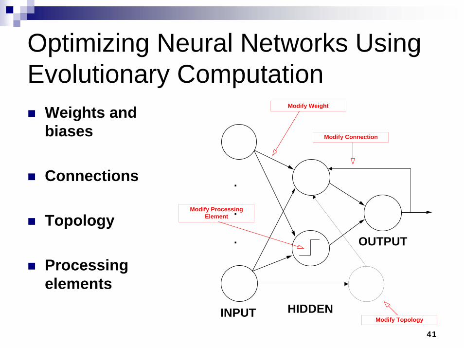
41
Optimizing Neural Networks Using Evolutionary Computation
Weights and biases
Connections
Topology
Processing elements
.
.
.
INPUT HIDDEN
OUTPUT
Modify Weight
Modify Connection
Modify Topology
Modify ProcessingElement
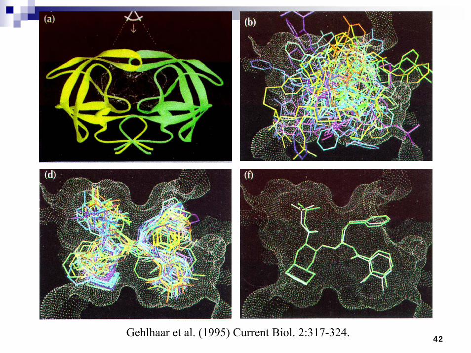
42Gehlhaar et al. (1995) Current Biol. 2:317-324.

43
Strategy for Broad-Spectrum Drug Discovery
Search nucleotide sequences for conserved RNA structures/drug targets with broad spectrum anti-bacterial or anti-viral activity

44
>105 hits
>105 hits
>105 hits
3-10
3-10
3-10
0-10 0-10
Exhaustive search for common
RNA structures infeasible
Organism A
Organism B
Organism C
Fogel et al., Nucl. Acids. Res. 30, 5310-5317 (2002) Macke et al., Nuc. Acids Res. 29, 4724-4735 (2001)

45
>105 hitsOrganism A
Structure A134Structure B56Structure C278
Bin #1
>105 hitsOrganism B
>105 hitsOrganism C
Structure A78Structure B9Structure C3567
Bin #2
Structure AxStructure ByStructure Cz
Bin #N
.
.
.
Scoring
Selection
Variation

46
Signal Recognition Particle –Domain IV
SRP targets signal peptide-containing proteins to plasma membranes (prokaryotes) or endoplasmic reticulum (eukaryotes)
Domain IV is essential, known binding site for protein component of SRP
Highly conserved, found over a wide phylogenetic distance
A AG A
G-CC-GU-G
G AG GA C
C AC-GC-GG-U
4-6
3-5 3-5
3
3

47
Experiment 1 2 3 4 5 6
Organism
H. sapiens 20 136 418 903 903 903A. fulgidus 15 69 200 724 724 724B. subtilis 12 62 374 520 520 520E. coli 14 45 258 523 523 523M. voltae 11 30 121 315 315 315S. pyogenes - - - - 57295 -S. aureus - - - - - 13591
Total 72 342 1371 2985 60280 16576
4-6
3-5 3-5
3
3
4-6
3-5 3-5
3-10
3-10
4-6
0-5 0-5
3-10
3-10
3-10
0-5 0-5
3-10
3-10
4-6
4-5
3
3
4-5

48
Signal Recognition Particle – Domain IV
Exp. Possible Bins P O G Time (min.) Fraction Evaluated1 5.5 × 10⁵ 80 40 3 2 1.7 × 10⁻²
2 7.9 × 10⁸ 80 40 7 4 2.8 × 10⁻⁵
3 9.8 × 10¹¹ 80 40 27 13 8.8 × 10⁻⁸
4 5.6 × 10¹³ 80 40 27 12 5.9 × 10⁻¹¹
5 3.2 × 10¹⁸ 200 100 25 90 1.5 × 10⁻¹³
6 7.6 × 10¹⁷ 200 100 13 41 3.4 × 10⁻¹³
gi|38795| |192 |24 |gcc cagg ccc ggaa ggg agca ggcgi|216348||153 |24 |tgt cagg tcc ggaa gga agca gcagi|42758| |204 |24 |ggt cagg tcc ggaa gga agca gccgi|177793||308 |24 |gcc cagg tcg gaaa cgg agca ggtgi|150042||310 |26 |ccg ccagg ccc ggaa ggg agcaa cgg
Experiments 1-4 A AG A
G-CC-GU-G
G AG GA C
C AC-GC-GG-U

49
Signal Recognition Particle – Domain IV
gi|38795| |192 |24 |gcc cagg ccc ggaa ggg agca ggcgi|216348| |153 |24 |tgt cagg tcc ggaa gga agca gcagi|42758| |204 |24 |ggt cagg tcc ggaa gga agca gccgi|177793| |308 |24 |gcc cagg tcg gaaa cgg agca ggtgi|150042| |310 |26 |ccg ccagg ccc ggaa ggg agcaa cgggb|AE004092| |190360 |24 |ggt cagg gga ggaa tcc agca gcc
gi|38795| |192 |24 |gcc cagg ccc ggaa ggg agca ggcgi|216348| |153 |24 |tgt cagg tcc ggaa gga agca gcagi|42758| |204 |24 |ggt cagg tcc ggaa gga agca gccgi|177793| |308 |24 |gcc cagg tcg gaaa cgg agca ggtgi|150042| |310 |26 |ccg ccagg ccc ggaa ggg agcaa cgggi|15922990| |525890 |24 |tgt cagg tcc tgac gga agca gca
A AG A
G-CC-GU-G
G AG GA C
C AC-GC-GG-U
Experiment 6
Experiment 5
50
Transcription Factor Binding Site (TFBS) Discovery
Use evolutionary computation to search for TFBSs of co-expressed genes
Identify known TFBS motifs as well as putative, previously unknown motifs that serve as promoters or enhancers
Follow up with experimental validation

51
Discovery of TFBSs using EC
Upstreamsequences
Evolve “window” placement
ATGCAAATATGTAAATATGTAAATATGCAAATATGCAAAGATGTAAAAATGCAAAT
Identify putative TFBSBased on sequence similarity
and complexityFogel et al. (2004) Nucl. Acids Res. 32(13):3826-3835
52
References – Bioinformatics Books
Mount, DW Bioinformatics: Sequence and Genome Analysis, Cold Spring Harbor Laboratory Press, 2001.Draghici, S Data Analysis Tools for DNA Microarrays, Chapman and Hall/CRC Press, 2003.Baldi, P and Brunak S Bioinformatics: The Machine Learning Approach, second ed., MIT Press, 2001.Westhead DR et al., Bioinformatics, BIOS Scientific Publishers Ltd., 2002.Gibas C and Jambeck P Developing Bioinformatics Computer Skills, O’Reilly, 2001.Augen, J Bioinformatics in the Post-Genomic Era: Genome, Transcriptome, Proteome, and Information-Based Medicine, Addison-Wesley, 2005.Branden C and Tooze J Introduction to Protein Structure, Garland Publishing, Inc. 1991.Jones NC and Pevzner PA An Introduction to Bioinformatics Algorithms, MIT Press, 2004.

53
ReferencesFogel GB and Corne DW Evolutionary Computation in Bioinformatics, Morgan Kauffman, 2003.Fogel GB “Microarray Data Mining with Evolutionary Computation,”in Evolutionary Computation in Data Mining, (A. Ghosh and LC Jain eds.) Springer, 2005Dybowski R and Gant V Clinical Applications of Artificial Neural Networks, Cambridge Univ. Press, 2001.Gehlhaar et al. (1995) Current Biol. 2:317-324Macke et al. (2001) Nuc. Acids Res. 29:4724-4735Fogel et al. (2002) Nuc. Acids Res. 30:5310-5317Weekes and Fogel (2003) BioSystems 72:149-158.Fogel et al. (2004) Nuc. Acids Res. 32:3826-3835DeRisi et al. (1997) Science 278:680-686

54
Tutorial on Evolutionary Computation in Bioinformatics: Part II
Gary B. FogelVice PresidentNatural Selection, Inc.9330 Scranton Rd., Suite 150San Diego, CA 92121 USA
Kay C. WieseSchool of Computing ScienceSimon Fraser UniversityCanadaChair: IEEE CIS Bioinformatics and Bioengineering Technical Committee
2007 IEEE Congress on Evolutionary Computation 2007 IEEE Congress on Evolutionary Computation -- September 25, 2007 September 25, 2007 -- SingaporeSingapore

55
OverviewComputational Intelligence (CI) in Bioinformatics RNA Structure and PredictionDesigning Algorithms Inspired by Nature: Evolutionary Computation – Successes in the RNA Domain with RnaPredictA comparison with known structures and mfoldjViz.Rna – A Dynamic RNA Visualization Tool Conclusions

56
Computational and Design Methods Used in Bioinformatics
Algorithm Design including: Dynamic ProgrammingHeuristic SearchComputational Intelligence Methods: Evolutionary Computation, Simulated Annealing, Neural Networks, Fuzzy Systems
Graphics and VisualizationDesigning models for sequence or structure information 2D and 3D visualization of structuresSystems design for input, output and manipulation Design of interactive input and output technology

57
Successful Applications of CI in Bioinformatics
Sequence AlignmentSAGA: An Evolutionary Algorithm (EA) for Sequence Alignment (Notredame et al.)
RNA Structure PredictionEvolutionary Algorithms (RnaPredict and PRnaPredict (Wiese et al., Shapiro et al., vanBatenburg et al.) Simulated Annealing

58
Successful Applications of CI in Bioinformatics, cont.
Protein Structure Prediction (Searching the Protein Conformational Space)
Evolutionary AlgorithmsSimulated AnnealingKnowledge Based Methods
Protein-Protein InteractionDo two proteins interact? Where? How?Searching Conformational Space for Docking (EAs)

59
Successful Applications of CI in Bioinformatics, cont.
Identify Coding Regions in DNAEvolved Artificial Neural Network for Gene Identification (Fogel et al.)
Excellent Overview of EA approaches in Bioinformatics
Evolutionary Computation in Bioinformatics, Gary B. Fogel and David W. Corne, Morgan Kaufmann Publishers (2003)Computational Intelligence in Bioinformatics, Fogel et al., IEEE Press (due Dec, 2007)
60
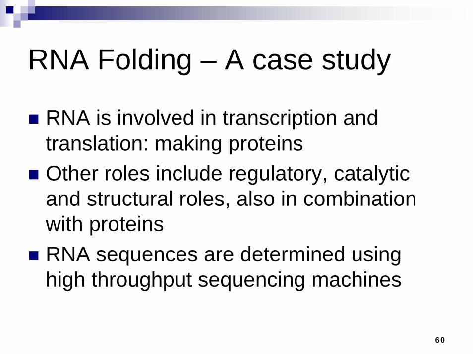
RNA Folding – A case study
RNA is involved in transcription and translation: making proteinsOther roles include regulatory, catalytic and structural roles, also in combination with proteinsRNA sequences are determined using high throughput sequencing machines

61
RNA Folding: Why should we care?
Why study/predict RNA structure?The structure of RNA molecules largely determines their function in the cell. Preservation of structure can be used to understand evolutionary processes. Knowing the structure or shape can be used to understand genetic diseases and to design new drugs.RNA secondary structure is formed by a natural folding process in which chemical bonds between certain so called canonical base pairs are formed.

62
RNA Folding
The canonical base pairs are GC, AU, GU, and mirrors CG, UA, UG
e.g.
Finding all canonical base pairs is simple, but which ones will actually form bonds ?
A U
5’ 3’

63
RNA Folding
While the sequence “folds” back onto itself it forms the secondary structure
A G C U G CU G U ACG U AA A
A G CU
GCU
GU
A
CG
UA
A
A
64
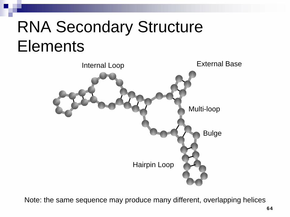
RNA Secondary Structure Elements
Hairpin Loop
Multi-loop
Internal Loop
Bulge
External Base
Note: the same sequence may produce many different, overlapping helices

65
RNA Double Helix Model
A helix consists of at least three consecutive canonical base pairs.The helix can only form if the sequence or loop connecting the two strands is at least 3 nucleotides long.
GGG CCC GGG CCC5’ 3’
66
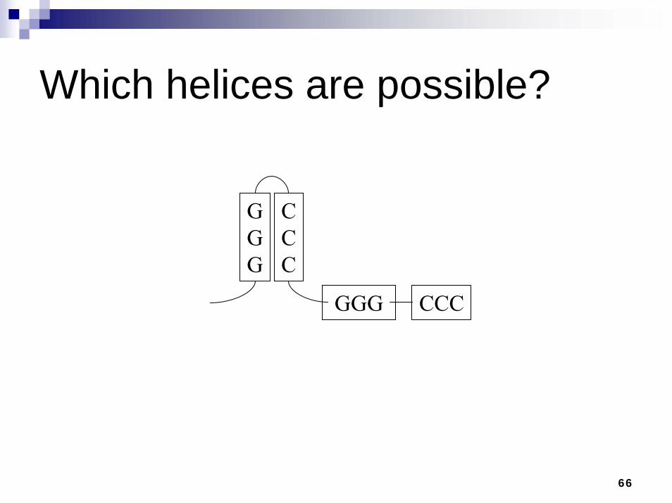
Which helices are possible?
GGG
CCC
GGG CCC

67
Which helices are possible?
GGG
CCC
GGG CCC
?
GGG
GGG
CCC
CCC
GGG CCC GGG CCC

68
RNA Folding by Energy Minimization
RNA molecules are stabilized by the formation of these helices (through base pair bonds).How do we know which helices will form?RNA molecules will fold into a minimum energystate. This minimum can be a local one.The free energy of a structure is determined by evaluating the thermodynamic model that is associated with the current structure.

69
RNA Thermodynamics
Energies for various RNA substructures can be determined experimentally and are associated with thermodynamic parameters. Thermodynamic models can consider bonding energies, stacking energies, and looping energies.Our work employs two stacking energy models
Individual Nearest Neighbor (INN) (Borer, Freier, Sugimoto, He)Individual Nearest Neighbor Hydrogen Bond (INN-HB) (Xia et al. 1998)

70
Free Energy Minimization Stacking Energies
Free energy (ΔG) is reduced as base pairs are formedTwo helices with same base pairs can have different ΔGΔG contribution of a base pair depends on
Position in helixProximity to other base pairs
Both INN and INN-HB model nearest-neighbors, terminal mismatches, dangling ends, helix initiation, and helix symmetry

71
Stacking Energies (INN and INN-HB)
A C
C G
G
U A
U
C
C G
A
( ) =Δ duplexG ⎟⎟⎠
⎞⎜⎜⎝
⎛ΔG
A
U A
U+
C
GA
U
⎟⎟⎠
⎞⎜⎜⎝
⎛ΔG
+initiationGΔ
+ symmetryGΔ
Suppose duplex:
⎟⎟⎠
⎞⎜⎜⎝
⎛ΔG
A
C
G
U+
72
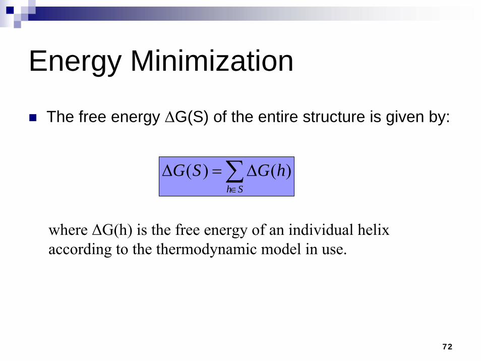
Energy Minimization
The free energy ΔG(S) of the entire structure is given by:
where ΔG(h) is the free energy of an individual helix according to the thermodynamic model in use.
)()( ∑∈
Δ=ΔSh
hGSG

73
Approach - Find All Pairs
1. Find all canonical base pairs2. Attempt to grow each pair(i,j) into a helix by
“stacking” pairs3. Add helix to set H of all potential helices
ACUAG U UC A UG G C
74
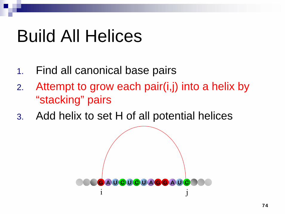
Build All Helices
1. Find all canonical base pairs2. Attempt to grow each pair(i,j) into a helix by
“stacking” pairs3. Add helix to set H of all potential helices
i jACUAG U UC A UG G C
75
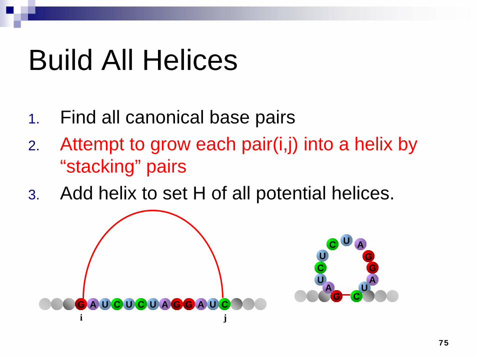
Build All Helices
1. Find all canonical base pairs2. Attempt to grow each pair(i,j) into a helix by
“stacking” pairs3. Add helix to set H of all potential helices.
AC
UG
C
U GU
CA
GU
i j
A
ACUAG U UC A UG G C

76
Build All Helices
1. Find all canonical base pairs2. Attempt to grow each pair(i,j) into a helix by
“stacking” pairs3. Add helix to set H of all potential helices
AC
UG
AC
U GU
CA
GU
i+1 j-1ACUAG U UC A UG G C
77
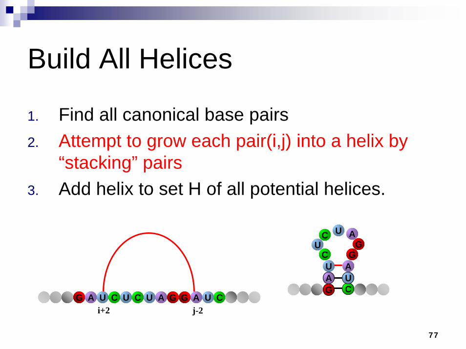
Build All Helices
1. Find all canonical base pairs2. Attempt to grow each pair(i,j) into a helix by
“stacking” pairs3. Add helix to set H of all potential helices.
A
CU
G
AC
UG
UC
A
GU
i+2 j-2ACUAG U UC A UG G C

78
Build All Helices
1. Find all canonical base pairs2. Attempt to grow each pair(i,j) into a helix by
“stacking” pairs3. Add helix to set H of all potential helices
AC
UG
AC
U G
U
CA
GU
i+3 j-3ACUAG U UC A UG G C
79
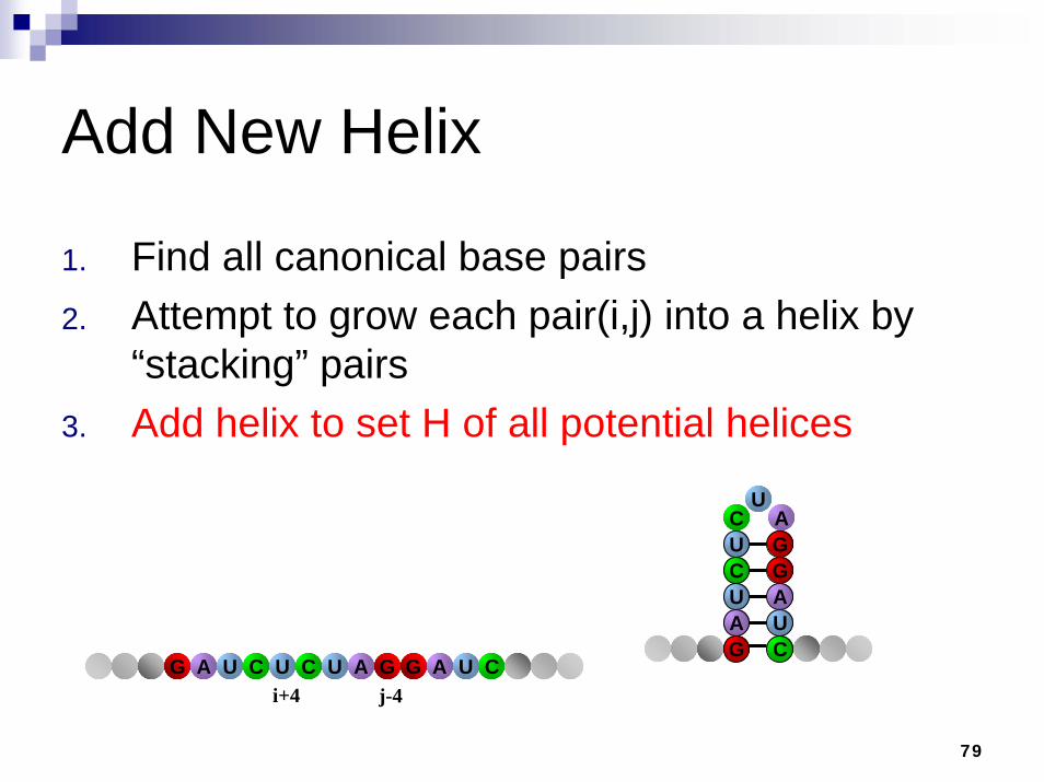
Add New Helix
1. Find all canonical base pairs2. Attempt to grow each pair(i,j) into a helix by
“stacking” pairs3. Add helix to set H of all potential helices
i+4 j-4ACUAG U UC A UG G C
ACU G
U
UG
AC
CA
GU

80
RNA Helices
Must have at least 3 “stacked” base pairsSequence or loop connecting the two strands must be at least 3 nucleotides longStore this new helix in a set H
i+4 j-4ACUAG U UC A UG G C
ACU G
U
UG
AC
CA
GU
81
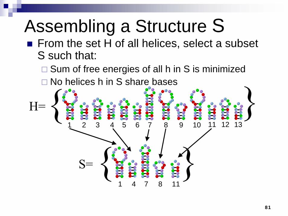
Assembling a Structure SFrom the set H of all helices, select a subset S such that:
Sum of free energies of all h in S is minimizedNo helices h in S share bases
S={ }{ }H=
1 2 3 4 5 6 7 8 9 10 11 12 13
111 4 7 8
82
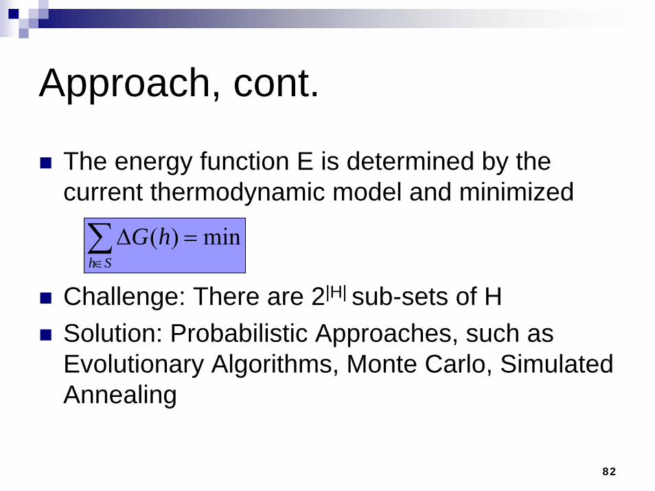
Approach, cont.
The energy function E is determined by the current thermodynamic model and minimized
Challenge: There are 2|H| sub-sets of HSolution: Probabilistic Approaches, such as Evolutionary Algorithms, Monte Carlo, Simulated Annealing
∑∈
=ΔSh
hG min)(

83
Objectives
To design a novel Evolutionary Algorithm to predict secondary RNA structure (RnaPredict)To evaluate the algorithm including convergence behavior and population dynamicsTo suggest several improvements to the algorithmTo study the effect of different selection and reproduction techniques on the EATo compare the outcome (predicted structures) with known structures and other approaches such as Nussinov and mfold
84
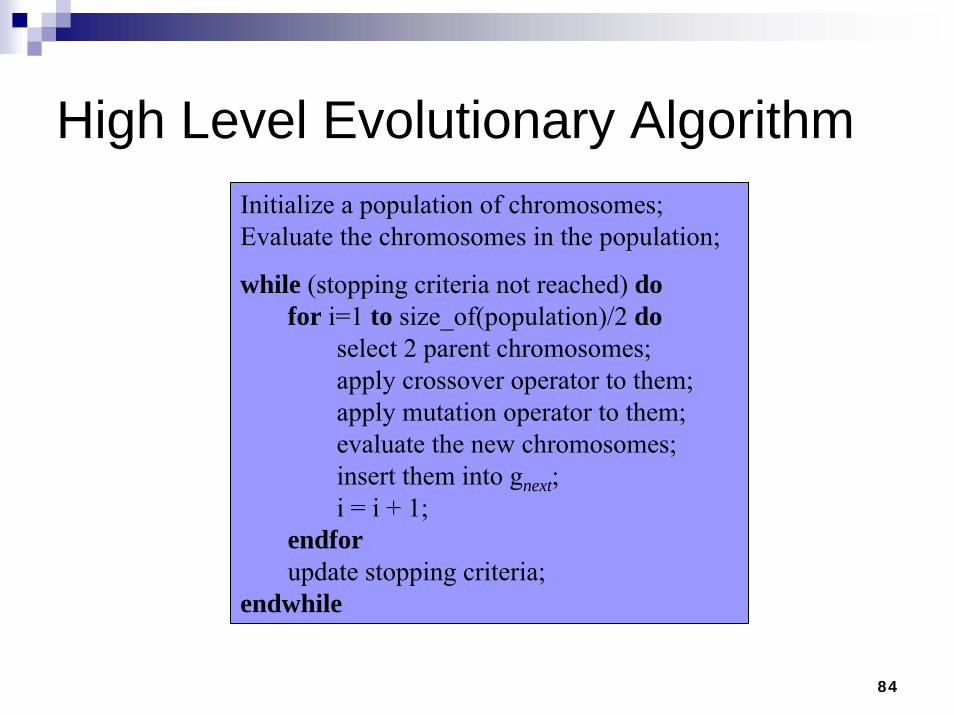
High Level Evolutionary AlgorithmInitialize a population of chromosomes;Evaluate the chromosomes in the population;
while (stopping criteria not reached) dofor i=1 to size_of(population)/2 do
select 2 parent chromosomes;apply crossover operator to them;apply mutation operator to them;evaluate the new chromosomes;insert them into gnext;i = i + 1;
endforupdate stopping criteria;
endwhile

85
Representing Structure S in the Algorithm
A permutation P of set H is used to represent the structure in the EA
{ }69 78 5 101113 123
Px=4
{ }69 78510 1113 1 23
Py=4
12
12

86
Decoding the PermutationWhen an individual is decoded, each helix in the permutation is iterated through
4
{ }6 781013 13
Sy=4
Only helices which do not conflict are scored and placed in the final structure
{ }68 1
Sx=12
87
Experiments and Results
Tested several sequences with both known and unknown structures4 selection/replacement strategies2 representations and 9 X-over operatorsover 100 combinations of Pc and PmPopulation size = 70030 independent runs with different random seeds785 nt human mRNA ...

88
Results – Roulette Wheel Selection
-1000
-950
-900
-850
-800
-750
-700
0 50 100 150 200 250 300 350 400# Generations
Free
Ene
rgy
(kca
l/mol
)
785 nt human mRNA, 10480 Possible Helices, Pm=5%, Pc=70%, pop_size = 700, CX, STDS, no elitism
89
Results: Keep-Best Reproduction
Faster convergenceBetter solution qualityWorks well with smaller population sizesVery robust over a wide range of operator probabilities

90
Results – KBR, cont.
785 nt human mRNA, 10480 Possible Helices, Pm=80%, Pc=70% pop_size = 700, CX, KBR, 1-elitism
-1000
-950
-900
-850
-800
-750
-700
0 50 100 150 200 250 300 350 400
# Generations
Free
Ene
rgy
(kca
l/mol
)

91
What about the structures?
So far we have focused on understanding the factors that control:
the convergence speed of the algorithm the effectiveness of the algorithm to find low energy structures
What about the actual structures? Need to know how close our predicted structures match real structures in nature

92
Predicted Structures vs. Real Structures
Haloarcula marismortui – 122nt
Correctly predicted base pairs
Bonding Model
Stacking Model (INN-HB)
Best <30% 71.1%
Best canonical base pairs only
41.3% 93.1%

93
What about the quality of the structures?
How much does the previous quantitative measure (base pair overlap) tell us? What do the structures look like?

94
Visualization of RNA secondary structure – jViz.Rna
We have developed a tool (jViz.Rna) to visualize RNA that could:
Be separate from the prediction tool Handle and display pseudo-knotsHave dynamic output for further manipulation by the userAllow for easy comparison of two structures Allow for quantitative comparison of two structuresAllow for saving the output as high quality graphics in a standard format (.gif)

95
jViz.Rna – Feynman diagramKnown Structure
KnownPredictedOverlap
Saccharomyces cerevisiae (Baker's Yeast) 118 nt

96
jViz.Rna – Predicted Structure
KnownPredictedOverlap
Saccharomyces cerevisiae (Baker's Yeast) 118 nt

97
jViz.Rna – Comparison of Predicted vs. Known Structure
KnownPredictedOverlap
Saccharomyces cerevisiae (Baker's Yeast) 118 nt
98
jViz.Rna – Dot Plot
KnownPredictedOverlap
Saccharomyces cerevisiae (Baker's Yeast) 118 nt

99
jViz.Rna – Classical Structure (known)
KnownPredictedOverlap
Saccharomyces cerevisiae(Baker's Yeast) 118 nt

100
jViz.Rna – Classical Structure (predicted)
KnownPredictedOverlap
Saccharomyces cerevisiae(Baker's Yeast) 118 nt

101
jViz.Rna – Overlaying predicted and known structure
KnownPredictedOverlap
Saccharomyces cerevisiae(Baker's Yeast) 118 nt

102
RNA Base Pairing
Canonical
G-C A-UG-U
Non-canonical
G-AA-AC-UU-Uand others…

103
Quantitative Overlap (known vs. predicted structure)
Known structure of Baker’s Yeast has a total of 37 bpsOur method RnaPredict predicts 33 of those (89.2%)Known structure contains 2 C-U pairs which cannot be predicted with the current model: 33/35 were found (94.3%)Without the C-U pairs the existing helix of size 3 would only be size 2 and could thus not be predictedOf the bps and helices that our model can predict, it found 100%, hence the search engine has a very high accuracy
104
A comparison with Nussinov DPA
Nussinov is a simplistic DPA for RNA secondary structure prediction that works on the principle of base pair maximizationModifications made to emulate bp weights at G-C = 3, A-U = 2, and G-U = 1Used as a base line for our comparisons
105
S. cerevisiae via Nussinov
Predicted
Overlap

106
Best Nussinov vs. best Correct BP EA run
Sequence Sequence Total BP
DPA over-pred.
EA over-pred.
DPA Corr. BPs
EA Corr. BPs
DPA Corr. BP %
EA Corr. BP %
S. cerevisiae 37 17 6 28 33 75.7% 89.2%H. marismortui 38 37 17 8 16 21.1% 71.1%
H. rubra 138 174 88 31 71 22.5% 51.4%D. virilis 233 291 168 29 66 12.4% 28.3%X. laevis 251 286 158 47 100 18.7% 39.8%

107
Best Nussinov vs. best Correct BP EA run
SequenceSequence Total BP
DPA over-pred.
EA over-pred.
DPA Corr. BPs
EA Corr. BPs
DPA Corr. BP %
EA Corr. BP %
A. lagunensis 113 142 59 30 73 26.5% 64.6%A. griffini 131 166 78 48 79 36.6% 60.3%
C. elegans 189 281 146 26 56 13.8% 29.6%H. sapiens 266 309 135 33 92 12.4% 34.6%
S. acidocaldarius 468 395 288 187 159 40.0% 34.0%

108
A comparison with mfoldmfold is the most cited and widely used RNA secondary structure prediction algorithm (based on DP)Developed by Zuker et al. Basic algorithm first introduced in 1981Since then refined continually until today (newest version published in 2003)Considered the gold standard of RNA secondary structure prediction

109
Overall Best Correct BP mfold vs. EA result
SequenceSequence Total BP
DPA over-pred.
EA over-pred.
DPA Corr. BPs
EA Corr. BPs
DPA Corr. BP %
EA Corr. BP %
S.cerevisiae 37 8 6 33 33 89.2% 89.2%H.marismortui 38 5 17 29 27 76.3% 71.1%
H.rubra 138 127 88 49 71 35.5% 51.4%D.virilis 233 199 168 37 66 15.9% 28.3%X.laevis 251 157 158 92 100 36.7% 39.8%
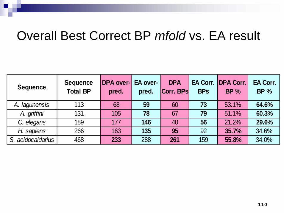
110
Overall Best Correct BP mfold vs. EA result
SequenceSequence Total BP
DPA over-pred.
EA over-pred.
DPA Corr. BPs
EA Corr. BPs
DPA Corr. BP %
EA Corr. BP %
A. lagunensis 113 68 59 60 73 53.1% 64.6%A. griffini 131 105 78 67 79 51.1% 60.3%
C. elegans 189 177 146 40 56 21.2% 29.6%H. sapiens 266 163 135 95 92 35.7% 34.6%
S. acidocaldarius 468 233 288 261 159 55.8% 34.0%

111
RnaPredict vs. mfold, cont.
2 extra base pairs predicted by mfold
KnownPredictedOverlap
Saccharomyces cerevisiae(Baker's Yeast) 118 nt

112
Pseudo-knots
2 base pairs (i, j) and (i’, j’) are pseudoknotted if i < i’ < j < j’… a 3D interaction. Occurrence of pseudo-knots is rather rare, but structurally significantTypically, longer sequences have a higher probability of having pseudo-knotsHow can we display them?
Arc and circular diagrams can display pseudo-knots but do not work well for longer sequencesClassical structure? Existing tools such as RnaViz do a poor job, example...

113
RnaVizH. rubra

114
jViz.Rna – Classical Structure and Pseudo-knots
Known H. rubra

115
Conclusions – RNA Folding
Excellent convergence behavior of EABest results achieved with Keep-Best Reproduction (both efficiency and quality of structures increase substantially)Very high accuracy of prediction for shorter sequencesEA is able to work with the “fuzziness” of the noisy thermodynamic model

116
Conclusion – RNA Folding cont.
Outperforms Nussinov DP in all but one case by a wide margin Outperforms mfold on several sequences,despite mfold’s use of a very sophisticated thermodynamic modelmfold also cannot predict non-canonical base pairs
117
Conclusion – jViz.RnajViz.Rna is a platform independent visualization tool for RNA structurejViz.Rna applications include:
study RNA structure evaluation of RNA folding algorithms

118
Venues of Interest
IEEE Symposium on Computational Intelligence in Bioinformatics and Comp. Biology (CIBCB) –www.cibcb.orgSpecial Session on EC in Bioinformatics and Comp. Biology at IEEE Congress on Evolutionary Computation.IEEE/ACM Transactions on Comp. Biology and BioinformaticsIEEE Transactions on NanoBioscienceIEEE Transactions on Evolutionary Computation

119
Acknowledgements
Simon Fraser UniversityNatural Science and Engineering Research Council of CanadaCanada Foundation for InnovationAndrew Hendriks –Presentation, Research and ProgrammingEdward Glen – Visualization of structuresAlain Deschenes – Research and Programming
Natural Selection, Inc.National Science FoundationNational Institutes of HealthDana Weekes, Mars Cheung –Research and ProgrammingInstitute of Electrical and Electronics Engineers IEEE and IEEE/CISL. Gwenn Volkert, Dan Ashlock, Clare Bates Congdon

120
Questions?

121
ReferencesDandekar, T. and Argos, P. (1996), "Ab initio tertiary-fold prediction of helical and non-helical protein chains using a genetic algorithm", International Journal of Biological Macromolecules, 18, pp. 1-4.Fogel, Gary B., and Corne David W. (2003), Evolutionary Computation in Bioinformatics, Morgan Kaufmann Publishers.Gultyaev AP, van Batenburg FHD, and Pleij CWA (1998), “RNA folding dynamics: Computer simulations by a genetic algorithm”, Molecular Modeling of Nucleic Acids, ACS Symposium Series, 682, pp. 229-245 Konig, Rainer and Dandekar, Thomas (1999), "Improving genetic algorithms for protein folding simulations by systematic crossover", BioSystems 50, pp. 17-25.Notredame, C. (2003), “Using Genetic Algorithms for Pairwise and Multiple Sequence Alignments”, in Evolutionary Computation in Bioinformatics (Gary B. Fogel and David W. Corn Eds.), Morgan Kaufmann Publishers, pp. 87 – 111.Pedersen, Jan T. and Moult, John (1996), "Genetic algorithms for protein structure prediction", Current Opinion in Structural Biology, 6 (2), 227-231Shapiro, B. A. and Navetta, J. (1994), A massively parallel genetic algorithm for RNA secondary structure prediction. The Journal of Supercomputing 8: 195-207.

122
References, cont.
Shapiro, B. A. and Wu, J. C. (1996) An annealing mutation operator in the genetic algorithms for RNA folding. Comput. Appl. Biosci. 12(3): 171-180.VanBatenburg F.H.D., Gultyaev A.P., and Pleij C.W.A. (1995), “An APL-programmed Genetic Algorithm for the Prediction of RNA Secondary Structure”, Journal of theoretical Biology, 174(3), pp. 269-280.Wiese, Kay C. and Goodwin, Scott D. (2001), “Keep Best Reproduction: A Local Family Competition Selection Strategy and the Environment it Flourishes in”, Constraints, 6, p. 399-422.Wiese Kay C. and Hendriks Andrew G. (2006), “Comparison of P-RnaPredict and mfold - Algorithms for RNA Secondary Structure Prediction”, Bioinformatics, doi:10.1093/bioinformatics/btl043.Wiese, Kay C., Glen, E. and Vasudevan, A. (2005). "jViz.Rna - A Java Tool for RNA Secondary Structure Visualization", IEEE Transactions on NanoBioscience, Vol 4(3), pp. 212-218.Michael Zuker: http://bioinfo.math.rpi.edu