188

46. Humminbird Raw Sonar Data

46.1. Humminbird Echograms

1. Sound levels are generally measured in decibels:

When I = Io, decibels = 0. Note that as I decreases relative to Io, the decibles value becomes increasingly negative.

2. Decibels are often measured relative to some specific reference value (e.g., Io has a specific value). In sonar calculations, the term “dBW” is often used, where

dBW = strength in decibels relative to 1 Watt (e.g., Io = 1.0 W) Thus

power in dBW = 10log(power in W) Therefore, at 1000 W, dBW = 30, and at 1 W, dBW = 0.

3. For the 997SI and 9673D Humminbird units, the maximum power output from the transducers is 1000 W at the transducer face. Therefore, these transducers have a maximum power of 30 dBW.

4. Humminbird units record the received (or return) echo power, referred to as SV or the intensity of the backscattered sound, as a color RGB echogram. Although SV values can take on any real values from approximately -100 dB to 0 dB, values in an RGB echogram can only take integer intensity values from 0 to 255. Thus, SV values are mapped so that the weakest echo maps to 0 while the strongest does not exceed 255. The RGB colors are produced by scaling so that the echogram threshold is mapped to 0 and the maximum possible SV value is mapped to 255. As a result, the data from Humminbird units represent relative SV values rather than absolute values. The raw data from the Humminbird units is normalized such that it has a 70 dB dynamic range (e.g., from -70 dB to 0 dB). Using this information, we can determine an approximate relationship between SV values and RGB values:

5. In Humminbird echograms, the ping time (e.g., time between pings) in milliseconds can be

calculated as follows:

ping time = time[n + 1] - time[n] where time[n] and time[n+1] are the times of consecutive pings in an echogram.

6. Ping duration (also referred to as pulse width or pulse length) is the length of time that a sonar sound burst is transmitted into the water. Shorter ping durations provide better target separation, but cannot travel to great depths. Longer ping durations provide better depth penetration, but result in poorer target separation. Humminbird varies ping duration based on depth to optimize both target separation and depth performance. Ping duration can range from 10 to 100 μs.

189

7. The ping duration determines the amount of vertical depth resolution between targets that the sonar unit can achieve.

range resolution = [(ping duration)(speed of sound)]/2 From the manuals for the Humminbird units, the average target separation is approximately 0.0635 m. This works out to a ping duration of approximately 85 μs, as shown below:

ping duration = [2(0.0635 m)]/(1500 m/s) = 8.5 x 10-5

s = 85 μs 8. Although the maximum frequency of the Humminbird transducers is 455 or 800 kHz, their ping

receiver frequency is approximately 38 kHz or 38000 Hz. This means that the time taken for each receive cycle to complete is:

Thus, the bin, or sample, length for the Humminbird units is 26 μs.

9. The inter-transmit cycle (e.g., the time between pulses, including the ping and the time during which return echoes are detected) is approximately 2000 ping durations long:

10. The complete peak for a return echo is, on average, approximately 40 pulse widths (or ping durations) wide, with 20 pulse widths on each side of the peak maximum. Thus, most peaks occupy approximately 2% of the inter-transmit cycle, or

190

46.2. Humminbird Beam Widths and Equivalent Beam Angles

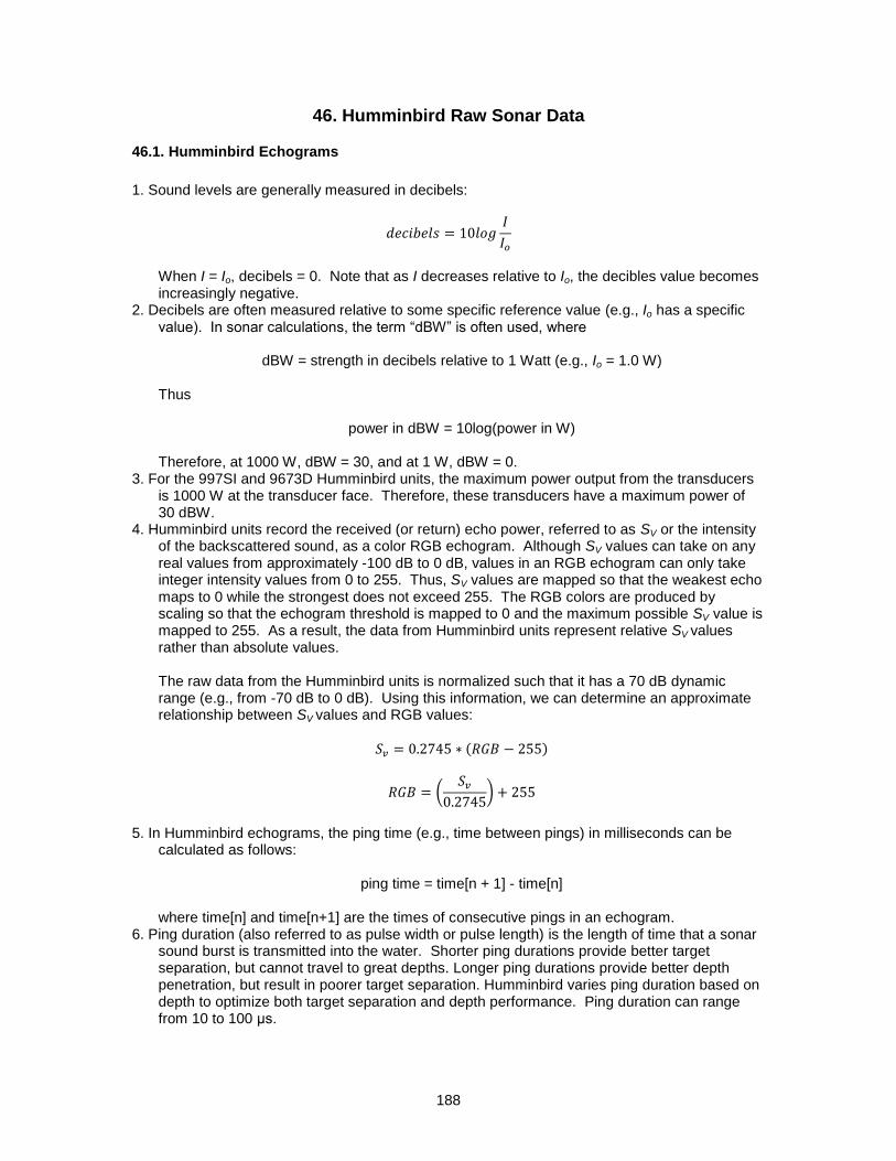
1. The schematic for a Humminbird side imaging transducer is shown below:

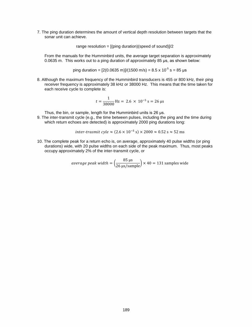
2. The beam coverage for a Humminbird side imaging sonar is shown below:

191

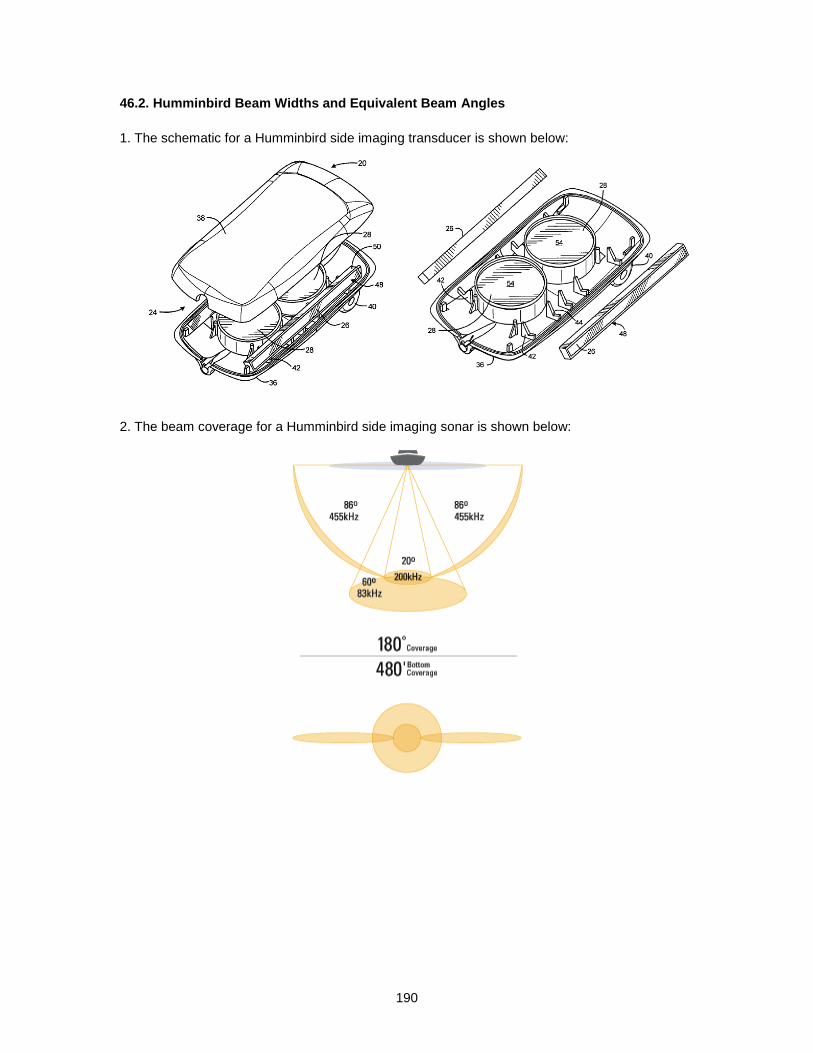
3. The schematic for a Humminbird 3D transducer is shown below:

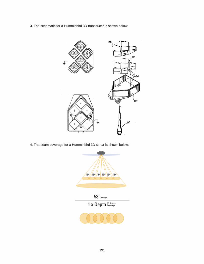
4. The beam coverage for a Humminbird 3D sonar is shown below:

192

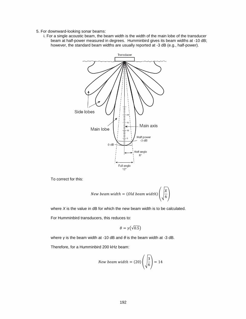
5. For downward-looking sonar beams: i. For a single acoustic beam, the beam width is the width of the main lobe of the transducer

beam at half-power measured in degrees. Humminbird gives its beam widths at -10 dB; however, the standard beam widths are usually reported at -3 dB (e.g., half-power).

To correct for this:

where X is the value in dB for which the new beam width is to be calculated. For Humminbird transducers, this reduces to:

where γ is the beam width at -10 dB and θ is the beam width at -3 dB. Therefore, for a Humminbird 200 kHz beam:

193

Therefore, for a Humminbird 83 kHz beam:

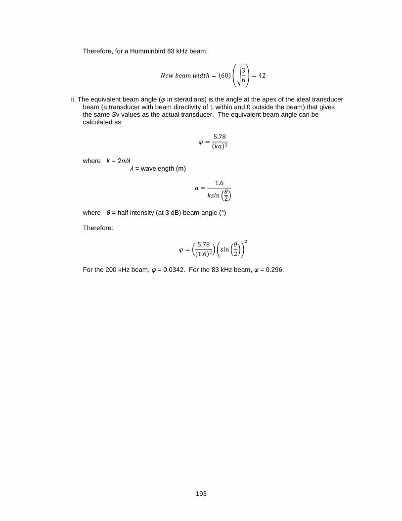
ii. The equivalent beam angle (φ in steradians) is the angle at the apex of the ideal transducer

beam (a transducer with beam directivity of 1 within and 0 outside the beam) that gives the same Sv values as the actual transducer. The equivalent beam angle can be calculated as

where k = 2π/λ λ = wavelength (m)

where θ = half intensity (at 3 dB) beam angle (°) Therefore:

For the 200 kHz beam, φ = 0.0342. For the 83 kHz beam, φ = 0.296.

194

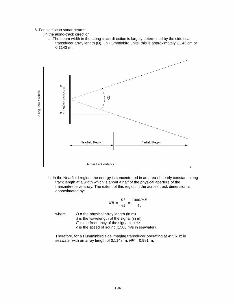
6. For side scan sonar beams: i. in the along-track direction:

a. The beam width in the along-track direction is largely determined by the side scan transducer array length (D). In Humminbird units, this is approximately 11.43 cm or 0.1143 m.

b. In the Nearfield region, the energy is concentrated in an area of nearly constant along

track length at a width which is about a half of the physical aperture of the transmit/receive array. The extent of this region in the across track dimension is approximated by:

where D = the physical array length (in m)

λ is the wavelength of the signal (in m) F is the frequency of the signal in kHz c is the speed of sound (1500 m/s in seawater)

Therefore, for a Humminbird side imaging transducer operating at 455 kHz in seawater with an array length of 0.1143 m, NR = 0.991 m.

195

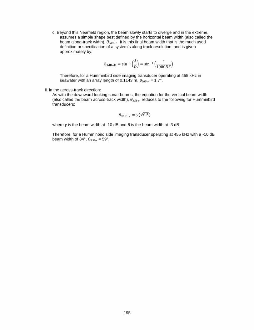
c. Beyond this Nearfield region, the beam slowly starts to diverge and in the extreme, assumes a simple shape best defined by the horizontal beam width (also called the beam along-track width), θ3dB-H. It is this final beam width that is the much used definition or specification of a system’s along track resolution, and is given approximately by:

Therefore, for a Humminbird side imaging transducer operating at 455 kHz in seawater with an array length of 0.1143 m, θ3dB-H = 1.7°.

ii. in the across-track direction: As with the downward-looking sonar beams, the equation for the vertical beam width (also called the beam across-track width), θ3dB-v, reduces to the following for Humminbird transducers:

where γ is the beam width at -10 dB and θ is the beam width at -3 dB. Therefore, for a Humminbird side imaging transducer operating at 455 kHz with a -10 dB beam width of 84°, θ3dB-v = 59°.

196

46.3. Some Echo Shape Parameters

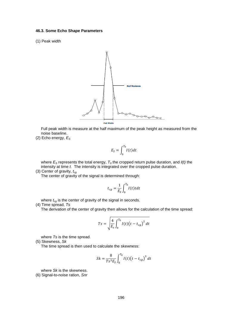
(1) Peak width

Full peak width is measure at the half maximum of the peak height as measured from the noise baseline.

(2) Echo energy, ES

where ES represents the total energy, T0 the cropped return pulse duration, and I(t) the intensity at time t. The intensity is integrated over the cropped pulse duration.

(3) Center of gravity, tcg The center of gravity of the signal is determined through:

where tcg is the center of gravity of the signal in seconds.

(4) Time spread, Ts The derivation of the center of gravity then allows for the calculation of the time spread:

where Ts is the time spread.

(5) Skewness, Sk The time spread is then used to calculate the skewness:

where Sk is the skewness.

(6) Signal-to-noise ration, Snr

197

where E is the combined signal and noise power at the location of the echo peak and NE is noise power. Since:

this can be written:

where A is the combined signal and noise amplitude at the location of the echo peak and NA is noise amplitude.

Since the time spread and skewness are normalized by the energy, these parameters pure shape parameters. Additionally, the skewness is independent of echo duration since it is normalized by the third power of Ts.

46.4. Determining the Minimum Depth for Start of Peak Picking

Calculate the Nearfield region for the transducer at its operational frequency using the equation below:

where D = the physical array length (in m) - for the sidescan units, D = 0.1143 m; for the

multibeam units, D = 0.105 m λ is the wavelength of the signal (in m) F is the frequency of the signal in kHz c is the speed of sound (1500 m/s in seawater)

For acoustic measurements that depend on the assumption of Farfield conditions, the range should be at least 2NR. If the minimum depth for peak picking (a user set parameter) is less than 2NR, set the minimum depth to 2NR.

198

46.5. Humminbird Sonars and Time Varying Gain

The sonar equation states that for backscattering from a resolved target, the received echo excess, EE, for an active sound system can be expressed as:

EE = SL − 2TL + TS + DI − NL where SL is the source level, TL is the one way transmission loss including the spherical spreading and the absorption, TS is the target strength, DI is the sonar directivity index, and NL is the ambient noise level. Time-varied-gain (TVG) is indispensable feature in sonars used in fisheries research in order to compensate for transmission loss and make the echo level independent of a target range. For most sonar systems, including multibeam sonars, the transmission loss (TL) is compensated for by applying a TVG internally. Ideally, the TVG follows the expectation of the theoretical acoustic transmission loss for resolved targets:

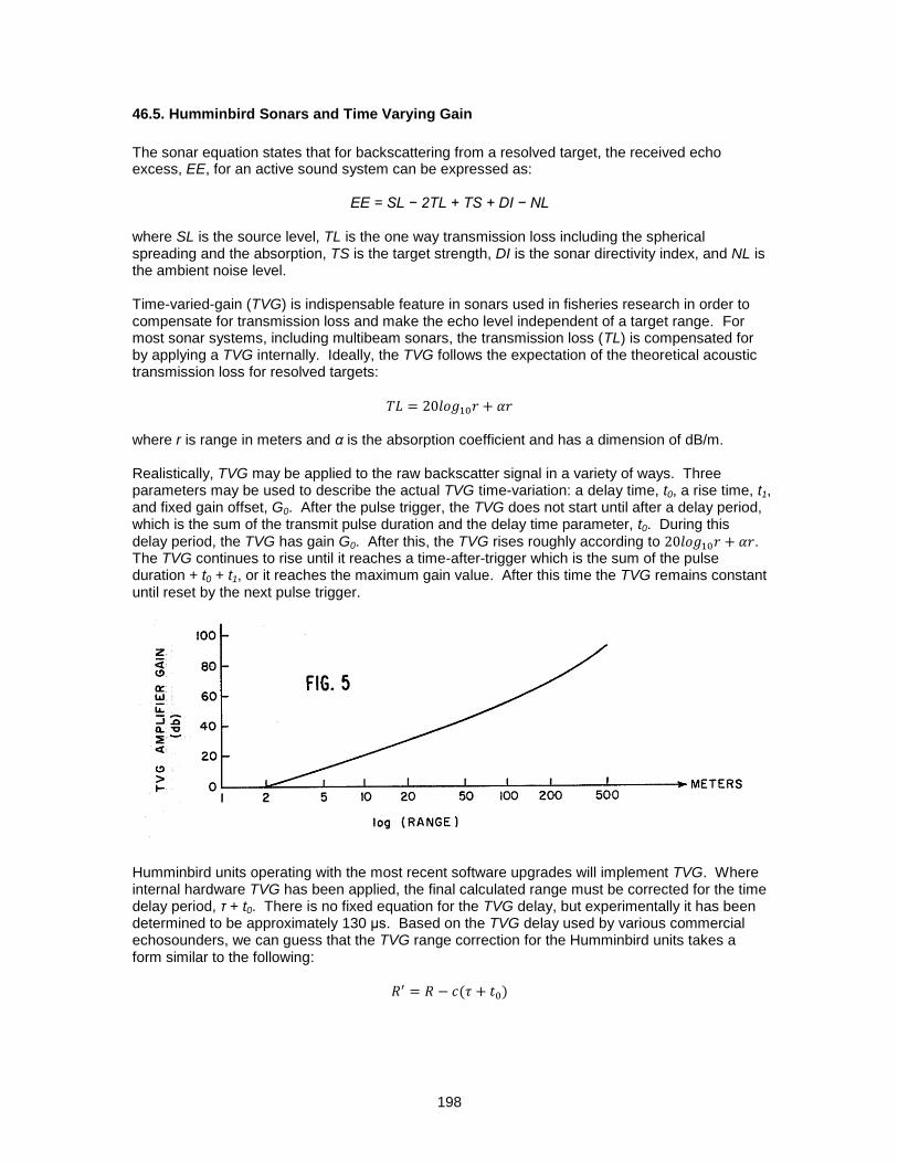
where r is range in meters and α is the absorption coefficient and has a dimension of dB/m. Realistically, TVG may be applied to the raw backscatter signal in a variety of ways. Three parameters may be used to describe the actual TVG time-variation: a delay time, t0, a rise time, t1, and fixed gain offset, G0. After the pulse trigger, the TVG does not start until after a delay period, which is the sum of the transmit pulse duration and the delay time parameter, t0. During this

delay period, the TVG has gain G0. After this, the TVG rises roughly according to . The TVG continues to rise until it reaches a time-after-trigger which is the sum of the pulse duration + t0 + t1, or it reaches the maximum gain value. After this time the TVG remains constant until reset by the next pulse trigger.

Humminbird units operating with the most recent software upgrades will implement TVG. Where internal hardware TVG has been applied, the final calculated range must be corrected for the time delay period, τ + t0. There is no fixed equation for the TVG delay, but experimentally it has been determined to be approximately 130 μs. Based on the TVG delay used by various commercial echosounders, we can guess that the TVG range correction for the Humminbird units takes a form similar to the following:

199

where R’ is the corrected range (m), R the uncorrected range (m), τ is the transmit pulse duration or pulse length, and c is the speed of sound. A variety of t0 values can be used, but the following value seems to best fit the observations:

where Δr is the range resolution (m) or the range occupied by one sample Thus, the TVG range correction is

For Humminbird units, Δr is the distance encompassed by one sample bin, and is equal to

τ is 85 μs. Thus, the TVG delay period can be reduced to

From this equation, the TVG time delay is 145 μs. If c = 1500 m/s (e.g., for saltwater), then the TVG range correction is is 0.22 m.

200

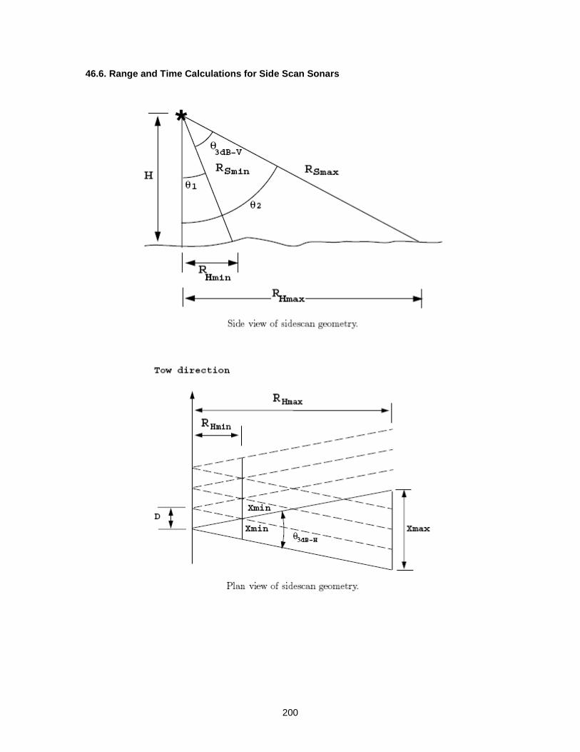
46.6. Range and Time Calculations for Side Scan Sonars

201

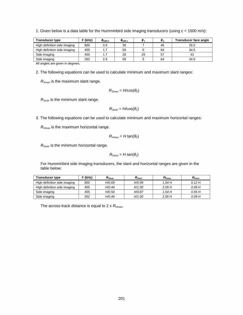
1. Given below is a data table for the Humminbird side imaging transducers (using c = 1500 m/s): Transducer type F (kHz) θ3dB-H θ3dB-v θ 1 θ 2 Transducer face angle

High definition side imaging 800 0.9 39 7 46 26.5

High definition side imaging 455 1.7 59 5 64 34.5

Side imaging 455 1.7 28 29 57 43

Side imaging 262 2.9 59 5 64 34.5

All angles are given in degrees.

2. The following equations can be used to calculate minimum and maximum slant ranges:

RSmax is the maximum slant range.

RSmax = H/cos(θ2) RSmin is the minimum slant range.

RSmin = H/cos(θ1) 3. The following equations can be used to calculate minimum and maximum horizontal ranges:

RHmax is the maximum horizontal range.

RHmax = H tan(θ2) RHmin is the minimum horizontal range.

RHmin = H tan(θ1) For Humminbird side imaging transducers, the slant and horizontal ranges are given in the table below:

Transducer type F (kHz) RSmax RSmin RHmax RHmin

High definition side imaging 800 H/0.69 H/0.99 1.04 H 0.12 H

High definition side imaging 455 H/0.44 H/1.00 2.05 H 0.09 H

Side imaging 455 H/0.54 H/0.87 1.54 H 0.55 H

Side imaging 262 H/0.44 H/1.00 2.05 H 0.09 H

The across-track distance is equal to 2 x RHmax.

202

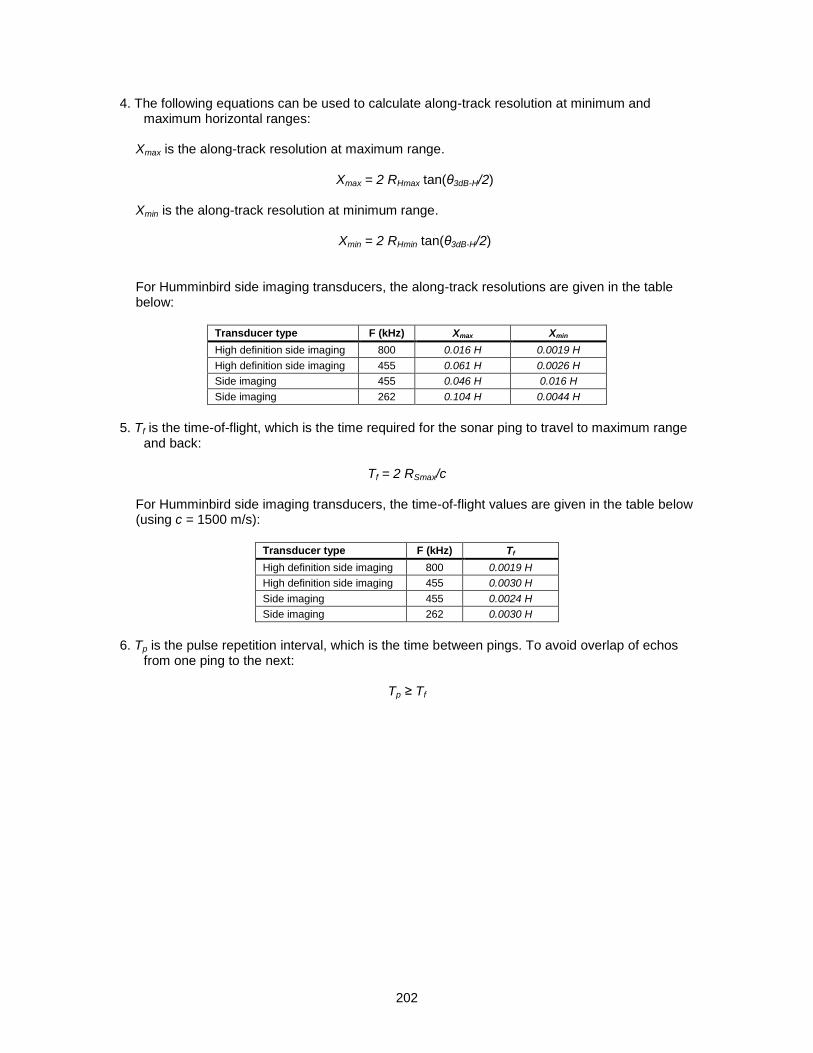
4. The following equations can be used to calculate along-track resolution at minimum and maximum horizontal ranges:

Xmax is the along-track resolution at maximum range.

Xmax = 2 RHmax tan(θ3dB-H/2) Xmin is the along-track resolution at minimum range.

Xmin = 2 RHmin tan(θ3dB-H/2) For Humminbird side imaging transducers, the along-track resolutions are given in the table below:

Transducer type F (kHz) Xmax Xmin

High definition side imaging 800 0.016 H 0.0019 H

High definition side imaging 455 0.061 H 0.0026 H

Side imaging 455 0.046 H 0.016 H

Side imaging 262 0.104 H 0.0044 H

5. Tf is the time-of-flight, which is the time required for the sonar ping to travel to maximum range

and back:

Tf = 2 RSmax/c For Humminbird side imaging transducers, the time-of-flight values are given in the table below (using c = 1500 m/s):

Transducer type F (kHz) Tf

High definition side imaging 800 0.0019 H

High definition side imaging 455 0.0030 H

Side imaging 455 0.0024 H

Side imaging 262 0.0030 H

6. Tp is the pulse repetition interval, which is the time between pings. To avoid overlap of echos

from one ping to the next:

Tp ≥ Tf

203

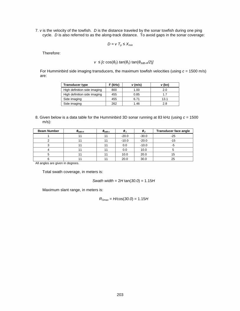
7. v is the velocity of the towfish. D is the distance traveled by the sonar towfish during one ping cycle. D is also referred to as the along-track distance. To avoid gaps in the sonar coverage:

D = v Tp ≤ Xmin

Therefore:

v ≤ [c cos(θ2) tan(θ1) tan(θ3dB-H/2)]

For Humminbird side imaging transducers, the maximum towfish velocities (using c = 1500 m/s) are:

Transducer type F (kHz) v (m/s) v (kn)

High definition side imaging 800 1.00 2.0

High definition side imaging 455 0.85 1.7

Side imaging 455 6.71 13.1

Side imaging 262 1.46 2.8

8. Given below is a data table for the Humminbird 3D sonar running at 83 kHz (using c = 1500

m/s):

Beam Number θ3dB-H θ3dB-v θ 1 θ 2 Transducer face angle

1 11 11 -20.0 -30.0 -25

2 11 11 -10.0 -20.0 -15

3 11 11 0.0 -10.0 -5

4 11 11 0.0 10.0 5

5 11 11 10.0 20.0 15

6 11 11 20.0 30.0 25

All angles are given in degrees.

Total swath coverage, in meters is:

Swath width = 2H tan(30.0) = 1.15H Maximum slant range, in meters is:

RSmax = H/cos(30.0) = 1.15H

204

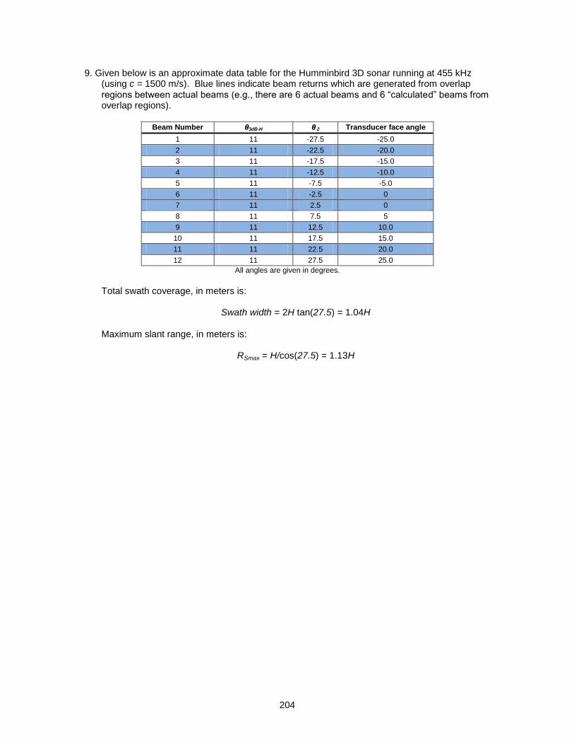
9. Given below is an approximate data table for the Humminbird 3D sonar running at 455 kHz (using c = 1500 m/s). Blue lines indicate beam returns which are generated from overlap regions between actual beams (e.g., there are 6 actual beams and 6 “calculated” beams from overlap regions).

Beam Number θ3dB-H θ 2 Transducer face angle

1 11 -27.5 -25.0

2 11 -22.5 -20.0

3 11 -17.5 -15.0

4 11 -12.5 -10.0

5 11 -7.5 -5.0

6 11 -2.5 0

7 11 2.5 0

8 11 7.5 5

9 11 12.5 10.0

10 11 17.5 15.0

11 11 22.5 20.0

12 11 27.5 25.0

All angles are given in degrees.

Total swath coverage, in meters is:

Swath width = 2H tan(27.5) = 1.04H Maximum slant range, in meters is:

RSmax = H/cos(27.5) = 1.13H

205

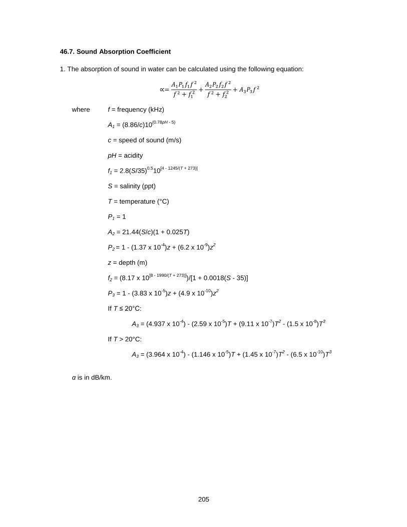
46.7. Sound Absorption Coefficient

1. The absorption of sound in water can be calculated using the following equation:

where f = frequency (kHz) A1 = (8.86/c)10

(0.78pH - 5)

c = speed of sound (m/s) pH = acidity f1 = 2.8(S/35)

0.510

[4 - 1245/(T + 273)]

S = salinity (ppt) T = temperature (°C) P1 = 1 A2 = 21.44(S/c)(1 + 0.025T) P2 = 1 - (1.37 x 10

-4)z + (6.2 x 10

-9)z

2

z = depth (m) f2 = (8.17 x 10

[8 - 1990/(T + 273)])/[1 + 0.0018(S - 35)]

P3 = 1 - (3.83 x 10

-5)z + (4.9 x 10

-10)z

2

If T ≤ 20°C: A3 = (4.937 x 10

-4) - (2.59 x 10

-5)T + (9.11 x 10

-7)T

2 - (1.5 x 10

-8)T

3

If T > 20°C: A3 = (3.964 x 10

-4) - (1.146 x 10

-5)T + (1.45 x 10

-7)T

2 - (6.5 x 10

-10)T

3

α is in dB/km.

206

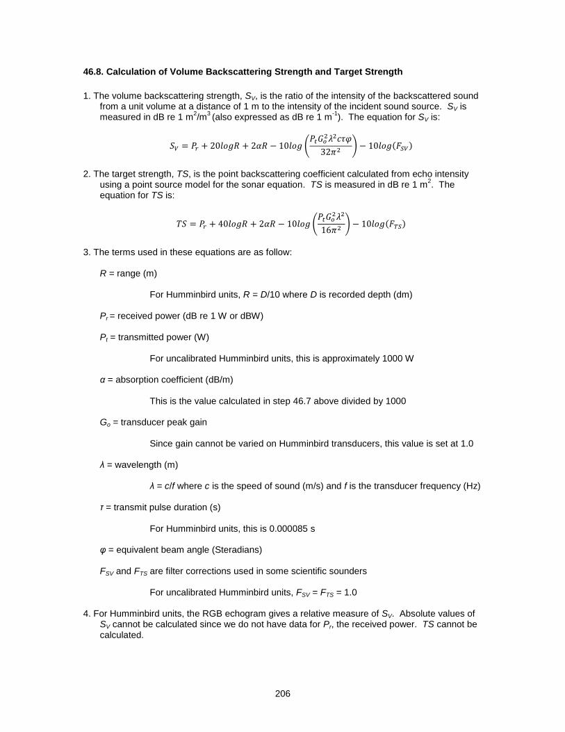
46.8. Calculation of Volume Backscattering Strength and Target Strength

1. The volume backscattering strength, SV, is the ratio of the intensity of the backscattered sound

from a unit volume at a distance of 1 m to the intensity of the incident sound source. SV is measured in dB re 1 m

2/m

3 (also expressed as dB re 1 m

-1). The equation for SV is:

2. The target strength, TS, is the point backscattering coefficient calculated from echo intensity

using a point source model for the sonar equation. TS is measured in dB re 1 m2. The

equation for TS is:

3. The terms used in these equations are as follow:

R = range (m) For Humminbird units, R = D/10 where D is recorded depth (dm) Pr = received power (dB re 1 W or dBW) Pt = transmitted power (W) For uncalibrated Humminbird units, this is approximately 1000 W α = absorption coefficient (dB/m) This is the value calculated in step 46.7 above divided by 1000 Go = transducer peak gain Since gain cannot be varied on Humminbird transducers, this value is set at 1.0 λ = wavelength (m) λ = c/f where c is the speed of sound (m/s) and f is the transducer frequency (Hz) τ = transmit pulse duration (s) For Humminbird units, this is 0.000085 s φ = equivalent beam angle (Steradians) FSV and FTS are filter corrections used in some scientific sounders For uncalibrated Humminbird units, FSV = FTS = 1.0

4. For Humminbird units, the RGB echogram gives a relative measure of SV. Absolute values of SV cannot be calculated since we do not have data for Pr, the received power. TS cannot be calculated.

207

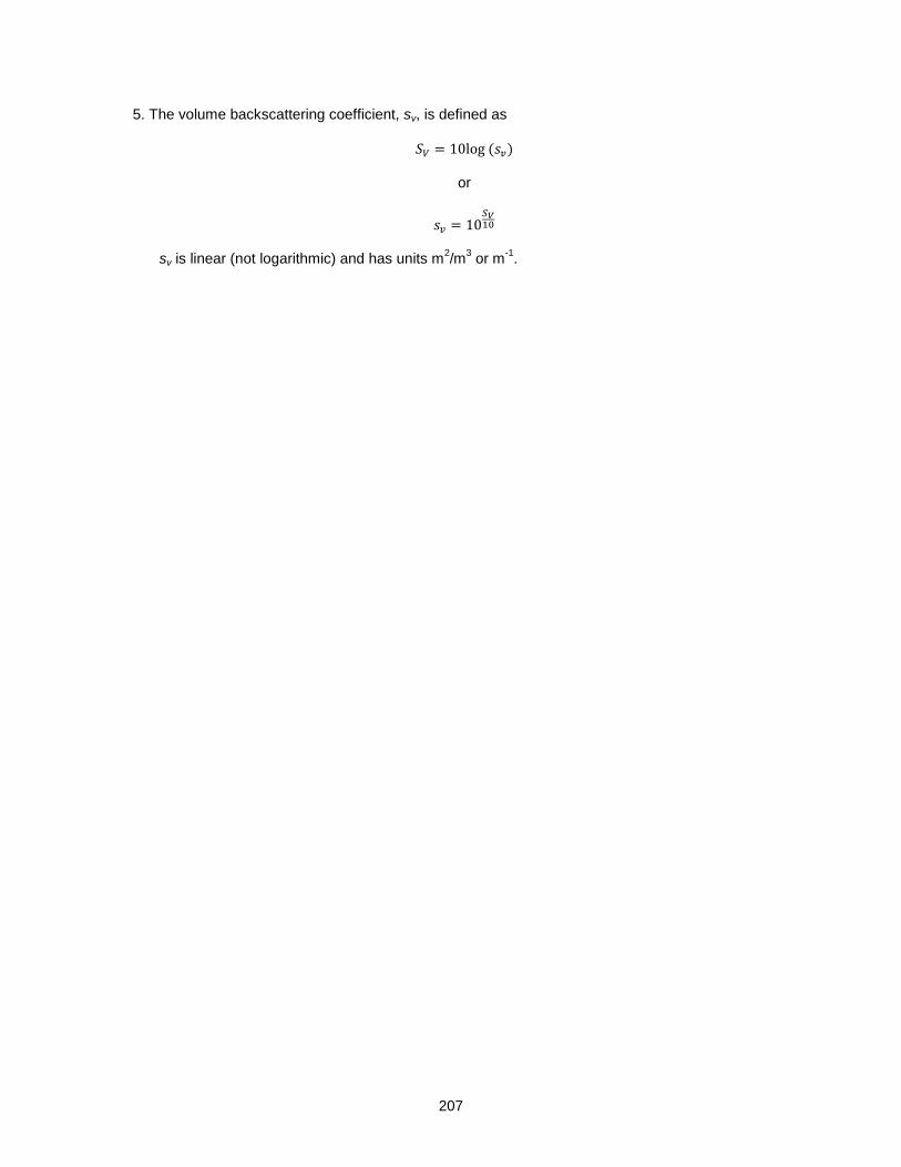
5. The volume backscattering coefficient, sv, is defined as

or

sv is linear (not logarithmic) and has units m

2/m

3 or m

-1.

208

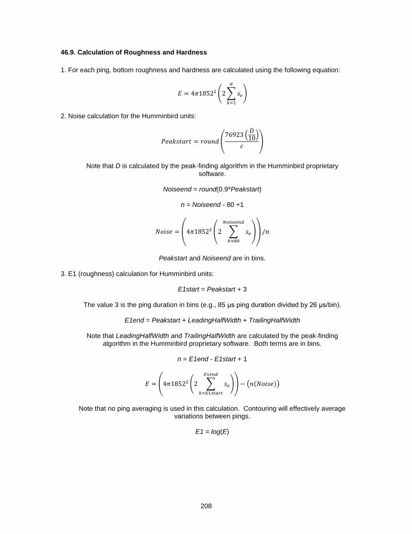
46.9. Calculation of Roughness and Hardness

1. For each ping, bottom roughness and hardness are calculated using the following equation:

2. Noise calculation for the Humminbird units:

Note that D is calculated by the peak-finding algorithm in the Humminbird proprietary

software.

Noiseend = round(0.9*Peakstart)

n = Noiseend - 80 +1

Peakstart and Noiseend are in bins.

3. E1 (roughness) calculation for Humminbird units:

E1start = Peakstart + 3

The value 3 is the ping duration in bins (e.g., 85 μs ping duration divided by 26 μs/bin).

E1end = Peakstart + LeadingHalfWidth + TrailingHalfWidth

Note that LeadingHalfWidth and TrailingHalfWidth are calculated by the peak-finding algorithm in the Humminbird proprietary software. Both terms are in bins.

n = E1end - E1start + 1

Note that no ping averaging is used in this calculation. Contouring will effectively average

variations between pings.

E1 = log(E)

209

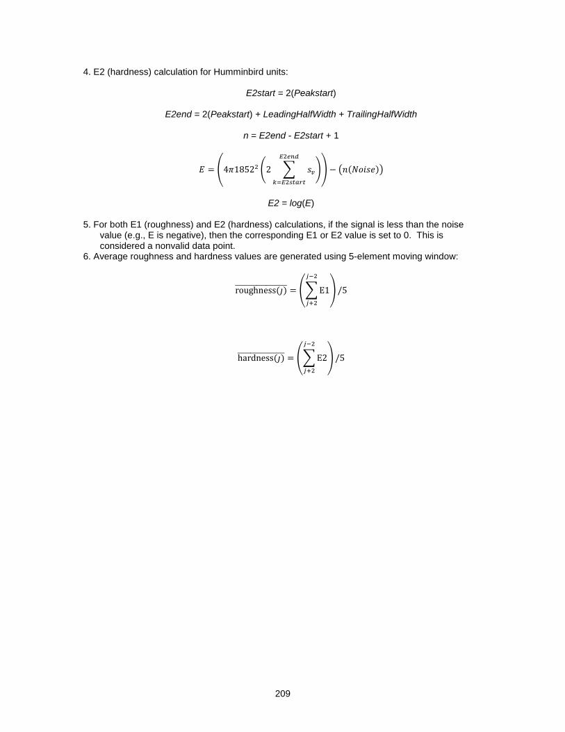
4. E2 (hardness) calculation for Humminbird units:

E2start = 2(Peakstart)

E2end = 2(Peakstart) + LeadingHalfWidth + TrailingHalfWidth

n = E2end - E2start + 1

E2 = log(E)

5. For both E1 (roughness) and E2 (hardness) calculations, if the signal is less than the noise

value (e.g., E is negative), then the corresponding E1 or E2 value is set to 0. This is considered a nonvalid data point.

6. Average roughness and hardness values are generated using 5-element moving window:

210

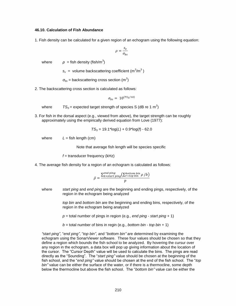
46.10. Calculation of Fish Abundance

1. Fish density can be calculated for a given region of an echogram using the following equation:

where ρ = fish density (fish/m

3)

sv = volume backscattering coefficient (m

2/m

3 )

σbs = backscattering cross section (m

2)

2. The backscattering cross section is calculated as follows:

where TSS = expected target strength of species S (dB re 1 m

2)

3. For fish in the dorsal aspect (e.g., viewed from above), the target strength can be roughly

approximately using the empirically derived equation from Love (1977):

TSS = 19.1*log(L) + 0.9*log(f) - 62.0

where L = fish length (cm) Note that average fish length will be species specific f = transducer frequency (kHz)

4. The average fish density for a region of an echogram is calculated as follows:

where start ping and end ping are the beginning and ending pings, respectively, of the

region in the echogram being analyzed

top bin and bottom bin are the beginning and ending bins, respectively, of the region in the echogram being analyzed p = total number of pings in region (e.g., end ping - start ping + 1) b = total number of bins in regin (e.g., bottom bin - top bin + 1)

“start ping”, “end ping”, “top bin”, and “bottom bin” are determined by examining the echogram using the SonarViewer software. These four values should be chosen so that they define a region which bounds the fish school to be analyzed. By hovering the cursur over any region in the echogram, a data box will pop up giving information about the location of the cursor. The “Cursor Depth” value will be used to calculate the bins. The pings are read directly as the “Sounding”. The “start ping” value should be chosen at the beginning of the fish school, and the “end ping” value should be chosen at the end of the fish school. The “top bin” value can be either the surface of the water, or if there is a thermocline, some depth below the thermocline but above the fish school. The “bottom bin” value can be either the

211

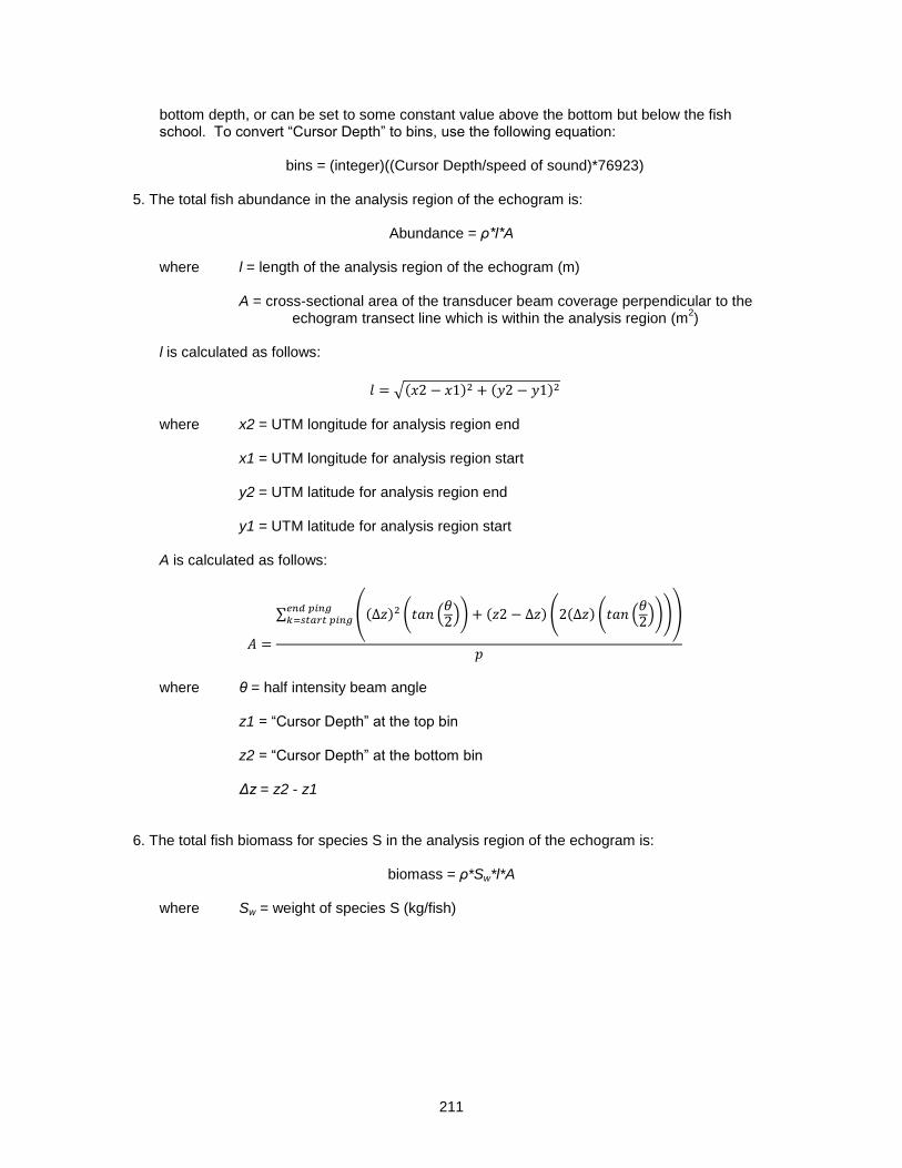
bottom depth, or can be set to some constant value above the bottom but below the fish school. To convert “Cursor Depth” to bins, use the following equation:

bins = (integer)((Cursor Depth/speed of sound)*76923)

5. The total fish abundance in the analysis region of the echogram is:

Abundance = ρ*l*A where l = length of the analysis region of the echogram (m) A = cross-sectional area of the transducer beam coverage perpendicular to the echogram transect line which is within the analysis region (m

2)

l is calculated as follows:

where x2 = UTM longitude for analysis region end x1 = UTM longitude for analysis region start y2 = UTM latitude for analysis region end y1 = UTM latitude for analysis region start A is calculated as follows:

where θ = half intensity beam angle z1 = “Cursor Depth” at the top bin z2 = “Cursor Depth” at the bottom bin Δz = z2 - z1

6. The total fish biomass for species S in the analysis region of the echogram is:

biomass = ρ*Sw*l*A

where Sw = weight of species S (kg/fish)

212

46.11. Calculation of Macrophyte Height

1. Bottom tracking is problematic in dense macrophyte beds. Acoustic reflections from the tops of

the plants can be so strong that the returns from the bottom are greatly diminished or entirely hidden. To avoid this problem, the bottom depth is determined over a range of 19 pings. Several common characteristics of macrophyte beds allow the bottom depth to be determined in this manner: i. At a rate of 10 pings per second, 19 pings occur in less than 2 seconds. At a typical towing

speed of under 3 knots, the distance covered during a 19 ping interval will be less than 3 m. In the lentic environments typically inhabited by macrophytes such as seagrasses, the bottom depth changes very little, usually no more than several tenths of a meter, over a 3 m interval.

ii. If canopy forming macrophytes are present, then the height of the canopy, as measured with each ping, will typically vary widely from ping to ping.

iii. Even in dense macrophyte beds, there are gaps in the canopy which allow an unobstructed “view” of the bottom by a vertically-aimed transducer.

Under these conditions, if a histogram is made of the bottom depth over 19 pings, the most commonly occurring value (mode) will typically be the bottom.

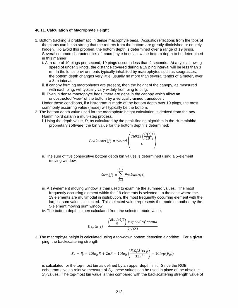
2. The bottom depth value used for the macrophyte height calculation is derived from the raw Humminbird data in a multi-step process. i. Using the depth value, D, as calculated by the peak-finding algorithm in the Humminbird

proprietary software, the bin value for the bottom depth is determined:

ii. The sum of five consecutive bottom depth bin values is determined using a 5-element

moving window:

iii. A 19-element moving window is then used to examine the summed values. The most

frequently occurring element within the 19 elements is selected. In the case where the 19 elements are multimodal in distribution, the most frequently occurring element with the largest sum value is selected. This selected value represents the mode smoothed by the 5-element moving sum window.

iv. The bottom depth is then calculated from the selected mode value:

3. The macrophyte height is calculated using a top-down bottom detection algorithm. For a given

ping, the backscattering strength

is calculated for the top-most bin as defined by an upper depth limit. Since the RGB echogram gives a relative measure of SV, these values can be used in place of the absolute SV values. The top-most bin value is then compared with the backscattering strength value of

213

the next deepest bin. backscattering strength difference

= - (backscattering strength[bini] - backscattering strength[bini-1]) If the backscattering strength difference is greater than a supplied vegetation threshold value, the top of the vegetation is assumed to start at bini. This process of comparing two consecutive bins is repeated for deeper and deeper bins until either the vegetation threshold value is exceeded or the bottom depth is reached.

4. Once the vegetation threshold value is exceeded, the program then checks to see over how many consecutive deeper bins the vegetation threshold value continues to be exceeded. If the number of consecutive bins over which the vegetation threshold is exceeded is larger than a user defined “vegetation bin width value”, macrophyte presence is declared and the vegetation height is calculated.

5. If the vegetation threshold value is exceeded for the required number of bins, the depth at which the vegetation starts is calculated using the bini value at which the threshold was first exceeded, and the total vegetation height (from roots to tip of shoots) is assumed to be

vegetation height = bottom depth - vegetation start depth

6. Average vegetation height values are generated using 5-element moving window: