4.1 digital-to-digital conversion - kennesaw...

A computer network is designed to send information from one point to another. This information needs to be converted to either a digital signal or an analog signal for transmission. In this chapter, we discuss the first choice, conversion to digital signals; in Chapter 5, we discuss the second choice, conversion to analog signals.

We discussed the advantages and disadvantages of digital transmission over analog transmission in Chapter 3. In this chapter, we show the schemes and techniques that we use to transmit data digitally. First, we discuss digital-to-digital conversion techniques, methods which convert digital data to digital signals. Second, we discuss analog-to-digital conversion techniques, methods which change an analog signal to a digital signal. Finally, we discuss transmission modes.

4.1 DIGITAL-TO-DIGITAL CONVERSION In Chapter 3, we discussed data and signals. We said that data can be either digital or analog. We also said that signals that represent data can also be digital or analog. In this section, we see how we can represent digital data by using digital signals. The conversion involves three techniques: line coding, block coding, and scrambling. Line coding is always needed; block coding and scrambling may or may not be needed.

Line Coding Line coding is the process of converting digital data to digital signals. We assume that data, in the form of text, numbers, graphical images, audio, or video, are stored in computer memory as sequences of bits (see Chapter 1). Line coding converts a sequence of bits to a digital signal. A t the sender, digital data are encoded into a digital signal; at the receiver, the digital data are recreated by decoding the digital signal. Figure 4.1 shows the process.

Characteristics

Before discussing different line coding schemes, we address their common characteristics.

101

Forouzan: Data I II. Physical Layer and I 4. Digital Transmission I I © T h e McGraw-Hill Communications and Media Companies, 2007 Networking, Fourth Edition

102 CHAPTER 4 DIGITAL TRANSMISSION

Figure 4.1 Line coding and decoding

Sender Receiver

m Digital data

0 I 0 1 • • • 1 0 I Digital signal

_ru~- LT Digital data

0 1 0 1 • • • 1 0 1

Link

Signal Element Versus Data Element Let us distinguish between a data element and a signal element. In data communications, our goal is to send data elements. A data element is the smallest entity that can represent a piece of information: this is the bit. In digital data communications, a signal element carries data elements. A signal element is the shortest unit (timewise) of a digital signal. In other words, data elements are what we need to send; signal elements are what we can send. Data elements are being carried; signal elements are the carriers.

We define a ratio r which is the number of data elements carried by each signal element. Figure 4.2 shows several situations with different values of r.

Figure 4.2 Signal element versus data element

1 data element

1 ! 0

J l signal I element

1 !

. One data element per one signal element (r = 1)

2 data elements

! 'I ! 01 ' 11 '

1 signal element

c. Two data elements per one signal element (r = 2)

1 data element

' 1 1 0 ' 1 1

i i i i

u~i_n_r 2 signal elements

b. One data element per two signal elements (r = -j)

4 data elements

i i

n o i ; i i

3 signal elements

d. Four data elements per three signal elements (r = -j)

In part a of the figure, one data element is carried by one signal element (r = 1). In part b of the figure, we need two signal elements (two transitions) to carry each data

Forouzan: Data I II. Physical Layer and I 4. Digital Transmission I I © The McGraw-Hill I Communications and Media Companies, 2007 Networking, Fourth Edition

SECTION 4.1 DIGITAL-TO-DIGITAL CONVERSION 103

element (r = i ) . We w i l l see later that the extra signal element is needed to guarantee synchronization. In part c of the figure, a signal element carries two data elements (r = 2). Finally, in part d, a group of 4 bits is being carried by a group of three signal elements (r = | ) . For every line coding scheme we discuss, we w i l l give the value of r.

A n analogy may help here. Suppose each data element is a person who needs to be carried from one place to another. We can think of a signal element as a vehicle that can carry people. When r = 1, it means each person is driving a vehicle. When r > 1, it means more than one person is travelling in a vehicle (a carpool, for example). We can also have the case where one person is driving a car and a trailer (r = | ) .

Data Rate Versus Signal Rate The data rate defines the number of data elements (bits) sent in Is. The unit is bits per second (bps). The signal rate is the number of signal elements sent in Is. The unit is the baud. There are several common terminologies used in the literature. The data rate is sometimes called the bit rate; the signal rate is sometimes called the pulse rate, the modulation rate, or the baud rate.

One goal in data communications is to increase the data rate while decreasing the signal rate. Increasing the data rate increases the speed of transmission; decreasing the signal rate decreases the bandwidth requirement. In our vehicle-people analogy, we need to carry more people in fewer vehicles to prevent traffic jams. We have a limited bandwidth in our transportation system.

We now need to consider the relationship between data rate and signal rate (bit rate and baud rate). This relationship, of course, depends on the value of r. It also depends on the data pattern. If we have a data pattern of all Is or all Os, the signal rate may be different from a data pattern of alternating Os and Is. To derive a formula for the relationship, we need to define three cases: the worst, best, and average. The worst case is when we need the maximum signal rate; the best case is when we need the minimum. In data communications, we are usually interested in the average case. We can formulate the relationship between data rate and signal rate as

S=cxNx - baud r

where N is the data rate (bps); c is the case factor, which varies for each case; S is the number of signal elements; and r is the previously defined factor.

Example 4.1

A signal is carrying data in which one data element is encoded as one signal element (r = 1). If the bit rate is 100 kbps, what is the average value of the baud rate if c is between 0 and 1?

Solution We assume that the average value of c is \ The baud rate is then

S=cxNx 1 = i xl00,000x i = 50,000 = 50kbaud r 2 1

Bandwidth We discussed in Chapter 3 that a digital signal that carries information is nonperiodic. We also showed that the bandwidth of a nonperiodic signal is continuous with an infinite range. However, most digital signals we encounter in real life have a

Forouzan: Data I II. Physical Layer and I 4. Digital Transmission I I © The McGraw-Hill Communications and Media Companies, 2007 Networking, Fourth Edition


bandwidth with finite values. In other words, the bandwidth is theoretically infinite, but many of the components have such a small amplitude that they can be ignored. The effective bandwidth is finite. From now on, when we talk about the bandwidth of a digital signal, we need to remember that we are talking about this effective bandwidth.

Although the actual bandwidth of a digital signal is infinite, the effective bandwidth is finite.

We can say that the baud rate, not the bit rate, determines the required bandwidth for a digital signal. If we use the transportation analogy, the number of vehicles affects the traffic, not the number of people being carried. More changes in the signal mean injecting more frequencies into the signal. (Recall that frequency means change and change means frequency.) The bandwidth reflects the range of frequencies we need. There is a relationship between the baud rate (signal rate) and the bandwidth. Bandwidth is a complex idea. When we talk about the bandwidth, we normally define a range of frequencies. We need to know where this range is located as wel l as the values of the lowest and the highest frequencies. In addition, the amplitude (if not the phase) of each component is an important issue. In other words, we need more information about the bandwidth than just its value; we need a diagram of the bandwidth. We w i l l show the bandwidth for most schemes we discuss in the chapter. For the moment, we can say that the bandwidth (range of frequencies) is proportional to the signal rate (baud rate). The minimum bandwidth can be given as

We can solve for the maximum data rate i f the bandwidth of the channel is given.

Example 4.2

The maximum data rate of a channel (see Chapter 3) is Nmax - 2XBX log 2 L (defined by the Nyquist formula). Does this agree with the previous formula for /V m a x ? Solution A signal with L levels actually can carry log 2 L bits per level. If each level corresponds to one signal element and we assume the average case (c = | ) , then we have

Nmsa=-xBxr = 2xBxlog2L

Baseline Wander ing In decoding a digital signal, the receiver calculates a running average of the received signal power. This average is called the baseline. The incoming signal power is evaluated against this baseline to determine the value of the data element. A long string of Os or Is can cause a drift in the baseline (baseline wandering) and make it difficult for the receiver to decode correctly. A good line coding scheme needs to prevent baseline wandering.

Forouzan: Data I II. Physical Layer and I 4. Digital Transmission

Communications and Media

Networking, Fourth Edition


D C Components When the voltage level in a digital signal is constant for a while, the spectrum creates very low frequencies (results of Fourier analysis). These frequencies around zero, called DC (direct-current) components, present problems for a system that cannot pass low frequencies or a system that uses electrical coupling (via a transformer). For example, a telephone line cannot pass frequencies below 200 H z . A l s o a long-distance l ink may use one or more transformers to isolate different parts of the line electrically. For these systems, we need a scheme with no DC component.

Self-synchronization To correctly interpret the signals received from the sender, the receiver's bit intervals must correspond exactly to the sender's bit intervals. If the receiver clock is faster or slower, the bit intervals are not matched and the receiver might misinterpret the signals. Figure 4.3 shows a situation in which the receiver has a shorter bit duration. The sender sends 10110001, while the receiver receives 110111000011.

Figure 4.3 Effect of lack of synchronization

>

1 1 0 0

0 1

i i • • . i i

1 | Time

a. Sent

i i i i i i i i i i i i

l l l i O i 1 i 1 i 1 < 0 « 0 I 0 i 0 t 1 i 1 I I I I I I I I I I I I

I I I I I Time

b. Received

A self-synchronizing digital signal includes timing information in the data being transmitted. This can be achieved i f there are transitions in the signal that alert the receiver to the beginning, middle, or end of the pulse. If the receiver's clock is out of synchronization, these points can reset the clock.

Example 4.3

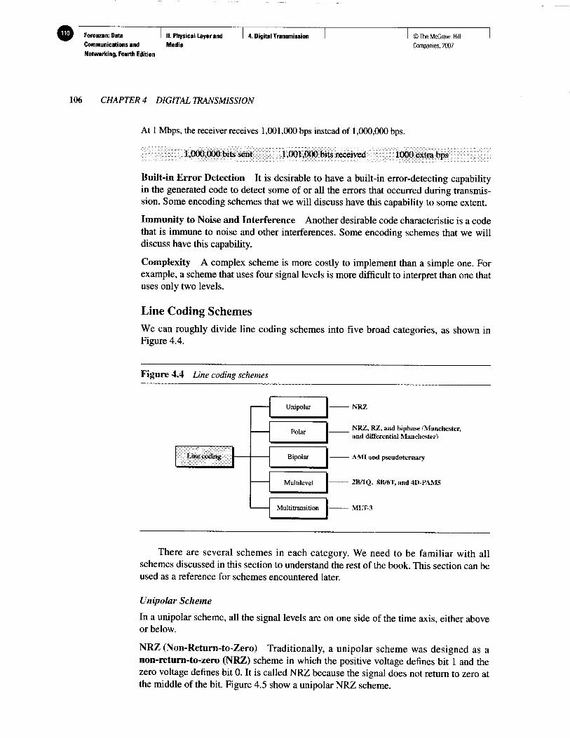
In a digital transmission, the receiver clock is 0.1 percent faster than the sender clock. How many extra bits per second does the receiver receive if the data rate is 1 kbps? How many if the data rate is 1 Mbps?

Solution At 1 kbps, the receiver receives 1001 bps instead of 1000 bps.

© T h e McGraw-Hill Companies. 2007

^ 0

1000 bits sent 1001 bits received 1 extra bps

Forouzan: Data

Communications and


II. Physical Layer and

Media

4. Digital Transmission © The McGraw-Hill Companies, 2007


At 1 Mbps, the receiver receives 1,001,000 bps instead of 1,000,000 bps.

1,000,000 bits sent 1,001,000 bits received 1000 extra bps

Bui l t - in E r r o r Detection It is desirable to have a built-in error-detecting capability in the generated code to detect some of or all the errors that occurred during transmission. Some encoding schemes that we w i l l discuss have this capability to some extent.

Immunity to Noise and Interference Another desirable code characteristic is a code that is immune to noise and other interferences. Some encoding schemes that we w i l l discuss have this capability.

Complexity A complex scheme is more costly to implement than a simple one. For example, a scheme that uses four signal levels is more difficult to interpret than one that uses only two levels.

Line Coding Schemes We can roughly divide line coding schemes into five broad categories, as shown in Figure 4.4.

Figure 4.4 Line coding schemes

Line coding

Unipolar

Polar

Bipolar

Multilevel

Multitransition

N R Z

N R Z , R Z . and biphase (Manchester, and differential Manchester)

A M I and pscudoternary

2B/1Q. 8B/6T. and 4D-PAM5

M L T - 3

There are several schemes in each category. We need to be familiar with a l l schemes discussed in this section to understand the rest of the book. This section can be used as a reference for schemes encountered later.

Unipolar Scheme

In a unipolar scheme, all the signal levels are on one side of the time axis, either above or below.

N R Z (Non-Return-to-Zero) Traditionally, a unipolar scheme was designed as a non-return-to-zero ( N R Z ) scheme in which the positive voltage defines bit 1 and the zero voltage defines bit 0. It is called N R Z because the signal does not return to zero at the middle of the bit. Figure 4.5 show a unipolar N R Z scheme.



Figure 4.5 Unipolar NRZ scheme

Amplitude

1 i 0 i 1 1 i 0

\v2 + i ( 0 ) 2 = i v 2

Time Normalized power

Compared with its polar counterpart (see the next section), this scheme is very costly. A s we w i l l see shortly, the normalized power (power needed to send 1 bit per unit line resistance) is double that for polar N R Z . For this reason, this scheme is normally not used in data communications today.

Polar Schemes

In polar schemes, the voltages are on the both sides of the time axis. For example, the voltage level for 0 can be positive and the voltage level for 1 can be negative.

Non-Return-to-Zero ( N R Z ) In polar NRZ encoding, we use two levels of voltage amplitude. We can have two versions of polar N R Z : N R Z - L and N R Z - I , as shown in Figure 4.6. The figure also shows the value of r, the average baud rate, and the bandwidth. In the first variation, N R Z - L (NRZ-Level), the level of the voltage determines the value of the bit. In the second variation, N R Z - I (NRZ-Invert), the change or lack of change in the level of the voltage determines the value of the bit. If there is no change, the bit is 0; i f there is a change, the bit is 1.

Figure 4.6 Polar NRZ-L and NRZ-I schemes

In NRZ-L the level of the voltage determines the value of the bit In NRZ-I the inversion or the lack of inversion determines the value of the bit

Let us compare these two schemes based on the criteria we previously defined. Although baseline wandering is a problem for both variations, it is twice as severe in N R Z - L . If there is a long sequence of Os or Is in N R Z - L , the average signal power



becomes skewed. The receiver might have difficulty discerning the bit value. In N R Z - I this problem occurs only for a long sequence of Os. If somehow we can eliminate the long sequence of Os, we can avoid baseline wandering. We wi l l see shortly how this can be done.

The synchronization problem (sender and receiver clocks are not synchronized) also exists in both schemes. Again , this problem is more serious in N R Z - L than in N R Z - I . Whi le a long sequence of Os can cause a problem in both schemes, a long sequence of Is affects only N R Z - L .

Another problem with N R Z - L occurs when there is a sudden change of polarity in the system. For example, i f twisted-pair cable is the medium, a change in the polarity of the wire results in all Os interpreted as Is and all Is interpreted as Os. N R Z - I does not have this problem. Both schemes have an average signal rate of N/2 B d .

NRZ-L and NRZ-I both have an average signal rate of N/2 Bd.

Let us discuss the bandwidth. Figure 4.6 also shows the normalized bandwidth for both variations. The vertical axis shows the power density (the power for each 1 Hz of bandwidth); the horizontal axis shows the frequency. The bandwidth reveals a very serious problem for this type of encoding. The value of the power density is very high around frequencies close to zero. This means that there are DC components that carry a high level of energy. A s a matter of fact, most of the energy is concentrated in frequencies between 0 and N/2. This means that although the average of the signal rate is N/2, the energy is not distributed evenly between the two halves.

NRZ-L and NRZ-I both have a DC component problem.

Example 4.4

A system is using NRZ-I to transfer 10-Mbps data. What are the average signal rate and minimum bandwidth?

Solution The average signal rate is S = N/2 = 500 kbaud. The minimum bandwidth for this average baud rate is = S = 500 kHz.

Return to Zero (RZ) The main problem with N R Z encoding occurs when the sender and receiver clocks are not synchronized. The receiver does not know when one bit has ended and the next bit is starting. One solution is the return-to-zero ( R Z ) scheme, which uses three values: positive, negative, and zero. In R Z , the signal changes not between bits but during the bit. In Figure 4.7 we see that the signal goes to 0 in the middle of each bit. It remains there until the beginning of the next bit. The main disadvantage of R Z encoding is that it requires two signal changes to encode a bit and therefore occupies greater bandwidth. The same problem we mentioned, a sudden change of polarity resulting in al l 0s interpreted as Is and all Is interpreted as 0s, still exist here, but there is no DC component problem. Another problem is the complexity: R Z uses three levels of voltage, which is more complex to create and discern. A s a result of all these deficiencies, the scheme is not used today. Instead, it has been replaced by the better-performing Manchester and differential Manchester schemes (discussed next).



Figure 4.7 Polar RZ scheme

Biphase: Manchester and Differential Manchester The idea of R Z (transition at the middle of the bit) and the idea of N R Z - L are combined into the Manchester scheme. In Manchester encoding, the duration of the bit is divided into two halves. The voltage remains at one level during the first half and moves to the other level in the second half. The transition at the middle of the bit provides synchronization. Differential Manchester, on the other hand, combines the ideas of R Z and N R Z - I . There is always a transition at the middle of the bit, but the bit values are determined at the beginning of the bit. If the next bit is 0, there is a transition; i f the next bit is 1, there is none. Figure 4.8 shows both Manchester and differential Manchester encoding.

Figure 4.8 Polar biphase: Manchester and differential Manchester schemes

Pis ~[_ 1 is J " ^

Manchester

0 0 i ! i

Time

i i

Differential i

Manchester —<

i

i i t

i Time

i

O No inversion: Next bit is 1 • Inversion: Next bit is 0

In Manchester and differential Manchester encoding, the transition at the middle of the bit is used for synchronization.

The Manchester scheme overcomes several problems associated with N R Z - L , and differential Manchester overcomes several problems associated with NRZ- I . First, there is no baseline wandering. There is no DC component because each bit has a positive and

Forouzan: Data I II. Physical Layer and I 4. Digital Transmission I I © The McGraw-Hill Communications and Media Companies, 2007 Networking. Fourth Edition


negative voltage contribution. The only drawback is the signal rate. The signal rate for Manchester and differential Manchester is double that for N R Z . The reason is that there is always one transition at the middle of the bit and maybe one transition at the end of each bit. Figure 4.8 shows both Manchester and differential Manchester encoding schemes. Note that Manchester and differential Manchester schemes are also called biphase schemes.

The minimum bandwidth of Manchester and differential Manchester is 2 times that of NRZ.

Bipolar Schemes

In bipolar encoding (sometimes called multilevel binary), there are three voltage levels: positive, negative, and zero. The voltage level for one data element is at zero, while the voltage level for the other element alternates between positive and negative.

In bipolar encoding, we use three levels: positive, zero, and negative.

A M I and Pseudotemary Figure 4.9 shows two variations of bipolar encoding: A M I and pseudotemary. A common bipolar encoding scheme is called bipolar alternate mark inversion (AMI). In the term alternate mark inversion, the word mark comes from telegraphy and means 1. So A M I means alternate 1 inversion. A neutral zero voltage represents binary 0. Binary Is are represented by alternating positive and negative voltages. A variation of A M I encoding is called pseudotemary in which the 1 bit is encoded as a zero voltage and the 0 bit is encoded as alternating positive and negative voltages.

Figure 4.9 Bipolar schemes: AMI and pseudotemary

Amplitude

AMI

Pseudotemary

o J i

Time

Time

The bipolar scheme was developed as an alternative to N R Z . The bipolar scheme has the same signal rate as N R Z , but there is no DC component. The N R Z scheme has most of its energy concentrated near zero frequency, which makes it unsuitable for transmission over channels with poor performance around this frequency. The concentration of the energy in bipolar encoding is around frequency N/2. Figure 4.9 shows the typical energy concentration for a bipolar scheme.




SECTION4.1 DIGITAL-TO-DIGITAL CONVERSION 111

One may ask why we do not have DC component in bipolar encoding. We can answer this question by using the Fourier transform, but we can also think about it intuitively. If we have a long sequence of Is, the voltage level alternates between positive and negative; it is not constant. Therefore, there is no DC component. For a long sequence of Os, the voltage remains constant, but its amplitude is zero, which is the same as having no DC component. In other words, a sequence that creates a constant zero voltage does not have a DC component.

A M I is commonly used for long-distance communication, but it has a synchronization problem when a long sequence of Os is present in the data. Later in the chapter, we w i l l see how a scrambling technique can solve this problem.

Multilevel Schemes

The desire to increase the data speed or decrease the required bandwidth has resulted in the creation of many schemes. The goal is to increase the number of bits per baud by encoding a pattern of m data elements into a pattern of n signal elements. We only have two types of data elements (Os and Is), which means that a group of m data elements can produce a combination of 2m data patterns. We can have different types of signal elements by allowing different signal levels. If we have L different levels, then we can produce Ln combinations of signal patterns. If 2m = Ln, then each data pattern is encoded into one signal pattern. If 2m < Ln, data patterns occupy only a subset of signal patterns. The subset can be carefully designed to prevent baseline wandering, to provide synchronization, and to detect errors that occurred during data transmission. Data encoding is not possible i f 2 m > Ln because some of the data patterns cannot be encoded.

The code designers have classified these types of coding as mBnL, where m is the length of the binary pattern, B means binary data, n is the length of the signal pattern, and L is the number of levels in the signaling. A letter is often used in place of L: B (binary) for L-2,T (ternary) for L = 3, and Q (quaternary) for L = 4. Note that the first two letters define the data pattern, and the second two define the signal pattern.

In mBnL schemes, a pattern of m data elements is encoded as a pattern of it signal elements in which 2m < L".

2B1Q The first mBnL scheme we discuss, two binary, one quaternary (2B1Q), uses data patterns of size 2 and encodes the 2-bit patterns as one signal element belonging to a four-level signal. In this type of encoding m = 2, n = 1, and L = 4 (quaternary). F i g ure 4.10 shows an example of a 2B1Q signal.

The average signal rate of 2B1Q is S = N/4. This means that using 2B1Q, we can send data 2 times faster than by using N R Z - L . However, 2B1Q uses four different signal levels, which means the receiver has to discern four different thresholds. The reduced bandwidth comes with a price. There are no redundant signal patterns in this scheme because 2 2 = 4 1 .

A s we w i l l see in Chapter 9, 2B1Q is used in D S L (Digital Subscriber Line) technology to provide a high-speed connection to the Internet by using subscriber telephone lines.

© The McGraw-H Companies, 2007

© Forouzan: Data I II. Physical Layer and I 4. Digital Transmission I I © The McGraw-Hill Communications and Media Companies. 2007 Networking, Fourth Edition


Figure 4.10 Multilevel: 2B1Q scheme

Previous level: Previous level: positive negative

Next Next Next bits level level

00 + 1 -1 01 +3 -3 10 -1 + 1 11 -3 +3

Transition table

0 0

+3 •

+ 1 •

-1 •

- 3 •

0 1 ! i o ' 0 1

Time

Assuming positive original level

Bandwidth

r*=-r 2 fIN

8B6T A very interesting scheme is eight binary, six ternary (8B6T). This code is used with 100BASE-4T cable, as we wi l l see in Chapter 13. The idea is to encode a pattern of 8 bits as a pattern of 6 signal elements, where the signal has three levels (ternary). In this type of scheme, we can have 2 8 = 256 different data patterns and 3 6 = 478 different signal patterns. The mapping table is shown in Appendix D. There are 478 - 256 = 222 redundant signal elements that provide synchronization and error detection. Part of the redundancy is also used to provide DC balance. Each signal pattern has a weight of 0 or +1 DC values. This means that there is no pattern with the weight - 1 . To make the whole stream DC-balanced, the sender keeps track of the weight. If two groups of weight 1 are encountered one after another, the first one is sent as is, while the next one is totally inverted to give a weight of - 1 .

Figure 4.11 shows an example of three data patterns encoded as three signal patterns. The three possible signal levels are represented as - , 0, and +. The first 8-bit pattern 00010001 is encoded as the signal pattern -0-0++ with weight 0; the second 8-bit pattern 01010011 is encoded as - + - + + 0 with weight +1. The third bit pattern should be encoded as + — + 0 + with weight +1. To create DC balance, the sender inverts the actual signal. The receiver can easily recognize that this is an inverted pattern because the weight is - 1 . The pattern is inverted before decoding.

Figure 4.11 Multilevel: 8B6T scheme

0 0 0 1 0 0 0 1 0 1 0 1 0 0 1 1 | 0 1 0 1 0 0 0 0 |

! inverted i pattern j

1 I Time

1

- 0 - 0 + + !

1 1

- + - + + 0 j + - - + 0 + !



The average signal rate of the scheme is theoretically 5 a v e = 1 x N x | ; in practice the minimum bandwidth is very close to 6 M 8 .

4 D - P A M 5 The last signaling scheme we discuss in this category is called four-dimensional five-level pulse amplitude modulation (4D-PAM5). The 4D means that data is sent over four wires at the same time. It uses five voltage levels, such as - 2 , - 1 , 0 , 1 , and 2. However, one level, level 0, is used only for forward error detection (discussed in Chapter 10). If we assume that the code is just one-dimensional, the four levels create something similar to 8B4Q. In other words, an 8-bit word is translated to a signal element of four different levels. The worst signal rate for this imaginary one-dimensional version is /Vx 4/8, or N/2.

The technique is designed to send data over four channels (four wires). This means the signal rate can be reduced to JV78, a significant achievement. A l l 8 bits can be fed into a wire simultaneously and sent by using one signal element. The point here is that the four signal elements comprising one signal group are sent simultaneously in a four-dimensional setting. Figure 4.12 shows the imaginary one-dimensional and the actual four-dimensional implementation. Gigabit L A N s (see Chapter 13) use this technique to send 1-Gbps data over four copper cables that can handle 125 Mbaud. This scheme has a lot of redundancy in the signal pattern because 2 8 data patterns are matched to 4 4 = 256 signal patterns. The extra signal patterns can be used for other purposes such as error detection.

Figure 4.12 Multilevel: 4D-PAM5 scheme

00011110 a

+ 2 -

+ 1 -

-1 -- 2 - •

1 Gbps 250 Mbps

•Wire 1 (125 MBd)

250 Mbps Wire 2 (125 MBd)

250 Mbps Wire 3 (125 MBd)

250 Mbps •Wire 4 (125 MBd)

Multiline Transmission: MLT-3

NRZ-I and differential Manchester are classified as differential encoding but use two transition rules to encode binary data (no inversion, inversion). If we have a signal with more than two levels, we can design a differential encoding scheme with more than two transition rules. MLT-3 is one of them. The multiline transmission, three level (MLT-3) scheme uses three levels (+V, 0, and - V ) and three transition rules to move between the levels.

1. If the next bit is 0, there is no transition.

2. If the next bit is 1 and the current level is not 0, the next level is 0.

3. If the next bit is 1 and the current level is 0, the next level is the opposite of the last nonzero level.



The behavior of M L T - 3 can best be described by the state diagram shown in Figure 4.13. The three voltage levels ( -V , 0, and +V) are shown by three states (ovals). The transition from one state (level) to another is shown by the connecting lines. Figure 4.13 also shows two examples of an M L T - 3 signal.

Figure 4.13 Multitransition: MLT-3 scheme

1 0 1 i 0 1 1 i 0 1 1

+v- 1 j +v-1

ov 1 ov 1 1

] Time

-v-\ 1 t -v-\ _ 1 1

a. Typical case

Next bit: 1

Next bit: 0

0 Next bit: 1

Next bit: 1

+V Last Last

non-zero non-zero NextbitO level: +V level:-V Next bit: 0

c Transition states

b. Worse case

One might wonder why we need to use M L T - 3 , a scheme that maps one bit to one signal element. The signal rate is the same as that for NRZ- I , but with greater complexity (three levels and complex transition rules). It turns out that the shape of the signal in this scheme helps to reduce the required bandwidth. Let us look at the worst-case scenario, a sequence of Is. In this case, the signal element pattern +V0 - V 0 is repeated every 4 bits. A nonperiodic signal has changed to a periodic signal with the period equal to 4 times the bit duration. This worst-case situation can be simulated as an analog signal with a frequency one-fourth of the bit rate. In other words, the signal rate for MLT-3 is one-fourth the bit rate. This makes MLT-3 a suitable choice when we need to send 100 Mbps on a copper wire that cannot support more than 32 M H z (frequencies above this level create electromagnetic emissions). MLT-3 and L A N s are discussed in Chapter 13.

Summary of Line Coding Schemes

We summarize in Table 4.1 the characteristics of the different schemes discussed.

Table 4.1 Summary of line coding schemes

Category Scheme Bandwidth (average) Characteristics

Unipolar NRZ B = N/2 Costly, no self-synchronization if long 0s or Is, D C

Unipolar

NRZ-L B = N/2 No self-synchronization if long Os or Is, D C

Unipolar NRZ-I B = N/2 No self-synchronization for long 0s, D C Unipolar

Biphase B = N Self-synchronization, no D C , high bandwidth





Table 4.1 Summary of line coding schemes (continued)

Category Scheme Bandwidth (average) Characteristics

Bipolar A M I B = N/2 No self-synchronization for long Os, D C

Multilevel

2B1Q B = N/4 No self-synchronization for long same double bits

Multilevel 8B6T B = 3N/4 Self-synchronization, no D C Multilevel

4D-PAM5 B = /W8 Self-synchronization, no D C

Multiline MLT-3 B = N/3 No self-synchronization for long Os

Block Coding We need redundancy to ensure synchronization and to provide some kind of inherent error detecting. Block coding can give us this redundancy and improve the performance of line coding. In general, block coding changes a block of m bits into a block of n bits, where n is larger than m. Block coding is referred to as an mBlnB encoding technique.

Block coding is normally referred to as mBlnB coding; it replaces each m-bit group with an n-bit group.

The slash in block encoding (for example, 4B/5B) distinguishes block encoding from multilevel encoding (for example, 8B6T), which is written without a slash. Block coding normally involves three steps: division, substitution, and combination. In the division step, a sequence of bits is divided into groups of m bits. For example, in 4B/5B encoding, the original bit sequence is divided into 4-bit groups. The heart of block coding is the substitution step. In this step, we substitute an m-bit group for an n-bit group. For example, in 4B/5B encoding we substitute a 4-bit code for a 5-bit group. Finally, the n-bit groups are combined together to form a stream. The new stream has more bits than the original bits. Figure 4.14 shows the procedure.

Figure 4.14 Block coding concept

Division of a stream into m-bit groups

m bits m bits m bits

1 1 0 ••• 1 0 0 0 ••• 1 • • • 0 1 0 ••• 1

mB-lo-nB substitution

I 0 1 0 ••• 101 0 0 0 ••• 0 0 1 • • • 0 1 1 ••• ! 1 1

nbits n bits n bits

Combining n-bit groups into a stream

© T h e McGraw-Hill Companies, 2007

©

Forouzan: Data

Communications and


II. Physical Layer and

Media

4. Digital Transmission © The McGraw-Hill Companies, 2007


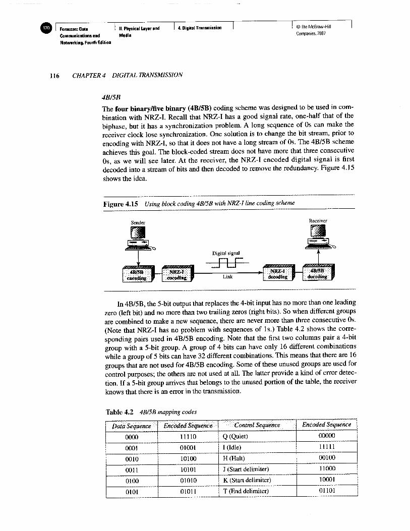
4B/5B

The four binary/five binary (4B/5B) coding scheme was designed to be used in combination with N R Z - I . Recal l that N R Z - I has a good signal rate, one-half that of the biphase, but it has a synchronization problem. A long sequence of Os can make the receiver clock lose synchronization. One solution is to change the bit stream, prior to encoding with N R Z - I , so that it does not have a long stream of Os. The 4B/5B scheme achieves this goal. The block-coded stream does not have more that three consecutive Os, as we w i l l see later. A t the receiver, the N R Z - I encoded digital signal is first decoded into a stream of bits and then decoded to remove the redundancy. Figure 4.15 shows the idea.

Figure 4.15 Using block coding 4B/5B with NRZ-I line coding scheme

Sender Receiver

Digital signal

-=FfcP Link

In 4B/5B, the 5-bit output that replaces the 4-bit input has no more than one leading zero (left bit) and no more than two trailing zeros (right bits). So when different groups are combined to make a new sequence, there are never more than three consecutive Os. (Note that N R Z - I has no problem with sequences of Is.) Table 4.2 shows the corresponding pairs used in 4B/5B encoding. Note that the first two columns pair a 4-bit group with a 5-bit group. A group of 4 bits can have only 16 different combinations while a group of 5 bits can have 32 different combinations. This means that there are 16 groups that are not used for 4B/5B encoding. Some of these unused groups are used for control purposes; the others are not used at all . The latter provide a kind of error detection. If a 5-bit group arrives that belongs to the unused portion of the table, the receiver knows that there is an error in the transmission.

Table 4.2 4B/5B mapping codes

Data Sequence Encoded Sequence Control Sequence Encoded Sequence

0000 11110 Q (Quiet) 00000

0001 01001 I (Idle) 11111

0010 10100 H (Halt) 00100

0011 10101 J (Start delimiter) 11000

0100 01010 K (Start delimiter) 10001

0101 01011 T (End delimiter) 01101

Forouzan: Data ! II. Physical Layer and I 4. Digital Transmission 1 I © The McGraw-Hill I Communications and Media Companies, 2007 Networking, Fourth Edition


Table 4.2 4B/5B mapping codes (continued)

Data Sequence Encoded Sequence Control Sequence Encoded Sequence

0110 OHIO S (Set) 11001

0111 01111 R (Reset) 00111

1000 10010

1001 10011

1010 10110

1011 10111

1100 11010

1101 11011

1110 11100

1111 11101

Figure 4.16 shows an example of substitution in 4B/5B coding. 4B/5B encoding solves the problem of synchronization and overcomes one of the deficiencies of N R Z - I . However, we need to remember that it increases the signal rate of N R Z - I . The redundant bits add 20 percent more baud. St i l l , the result is less than the biphase scheme which has a signal rate of 2 times that of N R Z - I . However, 4B/5B block encoding does not solve the DC component problem of N R Z - I . If a DC component is unacceptable, we need to use biphase or bipolar encoding.

Figure 4.16 Substitution in 4B/5B block coding

4-bit blocks

| 1 111 | • • • | 0 0 0 1 | [ 0 0 0 0 |

I I l I I [ | 1 1 1 1 0 ~] | I 1 I -.) I i • • • r_ 0 10 0 1 0 0 0 0 0

5-bit blocks

Example 4.5

We need to send data at a 1-Mbps rate. What is the minimum required bandwidth, using a combination of 4B/5B and NRZ-I or Manchester coding?

Solution First 4B/5B block coding increases the bit rate to 1.25 Mbps. The minimum bandwidth using NRZ-I is N/2 or 625 kHz. The Manchester scheme needs a minimum bandwidth of 1 MHz. The first choice needs a lower bandwidth, but has a D C component problem; the second choice needs a higher bandwidth, but does not have a D C component problem.

Forouzan: Data I II. Physical Layer and I 4. Digital Transmission I I © T h e McGraw-Hill Communications and Media Companies, 2007 Networking, Fourth Edition


8B/10B

The eight binary/ten binary (8B/10B) encoding is similar to 4B/5B encoding except that a group of 8 bits of data is now substituted by a 10-bit code. It provides greater error detection capability than 4B/5B. The 8B/10B block coding is actually a combination of 5B/6B and 3B/4B encoding, as shown in Figure 4.17.

Figure 4.17 8B/10B block encoding

8B/10B encoder

>-10-bit block

The most five significant bits of a 10-bit block is fed into the 5B/6B encoder; the least 3 significant bits is fed into a 3B/4B encoder. The split is done to simplify the mapping table. To prevent a long run of consecutive Os or Is, the code uses a disparity controller which keeps track of excess Os over Is (or Is over Os). If the bits in the current block create a disparity that contributes to the previous disparity (either direction), then each bit in the code is complemented (a 0 is changed to a 1 and a 1 is changed to a 0). The coding has 2 1 0 - 2 8 = 768 redundant groups that can be used for disparity checking and error detection. In general, the technique is superior to 4B/5B because of better built-in error-checking capability and better synchronization.

Scrambling Biphase schemes that are suitable for dedicated links between stations in a L A N are not suitable for long-distance communication because of their wide bandwidth requirement. The combination of block coding and N R Z line coding is not suitable for long-distance encoding either, because of the DC component. Bipolar A M I encoding, on the other hand, has a narrow bandwidth and does not create a DC component. However, a long sequence of Os upsets the synchronization. If we can find a way to avoid a long sequence of Os in the original stream, we can use bipolar A M I for long distances. We are looking for a technique that does not increase the number of bits and does provide synchronization. We are looking for a solution that substitutes long zero-level pulses with a combination of other levels to provide synchronization. One solution is called scrambling. We modify part of the A M I rule to include scrambling, as shown in Figure 4.18. Note that scrambling, as opposed to block coding, is done at the same time as encoding. The system needs to insert the required pulses based on the defined scrambling rules. Two common scrambling techniques are B8ZS and H D B 3 .

B8ZS

Bipolar with 8-zero substitution (B8ZS) is commonly used in North America. In this technique, eight consecutive zero-level voltages are replaced by the sequence

4.1 digital-to-digital conversion - kennesaw...

Documents