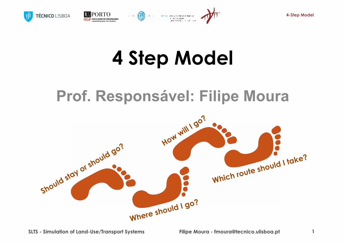
4 step model - ulisboa model theory of utility maximization: ... programs on travel demand. ......

4-Step Model

Prof. Responsável: Filipe Moura

4 Step Model

SLTS - Simulation of Land-Use/Transport Systems Filipe Moura - [email protected] 1

4-Step Model

The Modal Split Model (I)• Objective of Step 3

– Estimate the number of trips per available modes for each O/D pair of zones , separately

• The market shares are estimated with discrete choice models, based on the attractiveness of each mode, for each OD pair.– The attractiveness is quantified with the utility function of each mode for

each OD pair and, typically, include the attributes like travel time, no. of public transit transfers per trip, ease of parking, prices, etc., and of the preferences of the travelers

– Good practice suggests to avoid using more than 3 or 4 attributes for each mode, so that calibration is made on only a small number of parameters (although this is prone to discussion since computational performance has increased significantly in recent years)


4-Step Model

The Modal Split Model (II)Preparation of the modal split estimation:

1. The first step is to identify the set of available transport modes for each O/D pair (choice set per OD pair). Ø Walking should not be forgotten for shorter trips (<3km)!!!!

2. If information is enough, we should separate the O/D matrix according to 3 categories of travelers:a. Travelers who consider all available alternatives b. Those who do not have access to a private car and are captive of

public transport and/or walkingc. Those with extremely favorable conditions for private car use (e.g.,

company car and free parking place) will not consider other modes Ø Choice should be set differently for these 3 sets of travelers

3. Also their preferences and utility specifications will most likely be different, inasmuch as these groups will value differently the time spent (traveling + waiting), comfort, prices, etc.


4-Step Model

Theory of Utility Maximization: Utility• Utility U(Xi,Sn) is an indicator of value of an individual for one

alternative

– Depends on alternative-specific (AS) variables (Xi) for alternative i and socio-demographic (SD) characteristics (Sn) of an individual n

– If we assume linear relationships, it can be expressed as:

𝑈",$= 𝛽&'𝑋" + 𝛽'*𝑆$,where 𝛽&' and 𝛽'* are coefficients representing weights of the corresponding variables in the utility (these are tastes which vary across the individuals)

– Example of a bus utility function for an individual:

𝑈,-.= 𝛽/0𝑇𝑟𝑎𝑣𝑒𝑙𝐶𝑜𝑠𝑡 + 𝛽//𝑇𝑟𝑎𝑣𝑒𝑙𝑇𝑖𝑚𝑒 +𝛽>?@𝐴𝑔𝑒

AS SDSLTS - Simulation of Land-Use/Transport Systems Filipe Moura - [email protected] 4

4-Step Model

Theory of Utility Maximization: Decision Making

• Individual seeks to maximize the utility (assumption of rational decision making)

– Deterministic: an individual always choses the alternative with the highest utility, which is known• If U(Xi,Sn) ≥U(Xj,Sn), then individual n choses alternative i over

alternative j– Probabilistic: an individual always choses the alternative with

the highest utility, but we can only find a probability that the utility of one alternative is higher than the utility of another alternative for the given individual• P(U(Xi,Sn) ≥U(Xj,Sn)) – probability that i has higher utility than j for in

individual n• accommodates the analyst’s lack of information


4-Step Model

Probabilistic Utility• Assume that the utility for individual n and alternative i

consists of the two parts:𝑈"$=𝑉"$ + 𝜀"$,

Ø 𝑽𝒊𝒏 is the systematic utility and is a function of AS and SD observable variables

Ø 𝜺𝒊𝒏 is the random utility component, corresponds to the unobservable part of the utility function, including:• Unobserved variables (x)• Unobserved taste variations (β)• Measurement errors• Use of proxy variables

Ø Example of a bus utility function for an individual:

𝑈,-.= 𝛽/0𝑇𝑟𝑎𝑣𝑒𝑙𝐶𝑜𝑠𝑡 + 𝛽//𝑇𝑟𝑎𝑣𝑒𝑙𝑇𝑖𝑚𝑒 +𝛽>?@𝐴𝑔𝑒 + 𝜀,-.


𝑉"$- the systematic utility therandomcomponent

4-Step Model

Examples of DCM• Binary logit

Choice set (for each individual n)

• Multinomial logit - Choice set with 3 alternativesChoice set


4-Step Model

The Traffic Assignment Model (I)


DEMAND(OD matrix)

Supply(Network)

Assignment Models

Assignment

Simulation

FlowsDelays

Network performance indicators

❑ Objective of Step 4Ø Estimate how trips are allocated to different routes that connect each

mode for each OD pairØ The planner can get realistic estimates of the effects of policies and

programs on travel demand.

4-Step Model

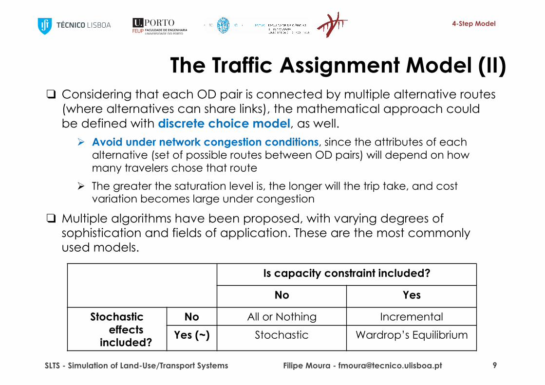
The Traffic Assignment Model (II)

Is capacity constraint included?

No Yes

Stochastic effects

included?

No All or Nothing IncrementalYes (~) Stochastic Wardrop’s Equilibrium


❑ Considering that each OD pair is connected by multiple alternative routes (where alternatives can share links), the mathematical approach could be defined with discrete choice model, as well.

Ø Avoid under network congestion conditions, since the attributes of each alternative (set of possible routes between OD pairs) will depend on how many travelers chose that route

Ø The greater the saturation level is, the longer will the trip take, and cost variation becomes large under congestion

❑ Multiple algorithms have been proposed, with varying degrees of sophistication and fields of application. These are the most commonly used models.

4-Step Model

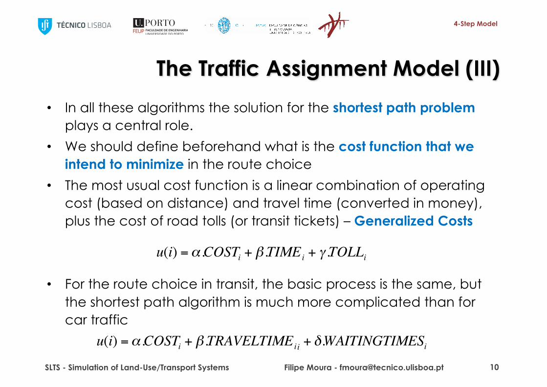
The Traffic Assignment Model (III)• In all these algorithms the solution for the shortest path problem

plays a central role.• We should define beforehand what is the cost function that we

intend to minimize in the route choice• The most usual cost function is a linear combination of operating

cost (based on distance) and travel time (converted in money), plus the cost of road tolls (or transit tickets) – Generalized Costs

• For the route choice in transit, the basic process is the same, but the shortest path algorithm is much more complicated than for car traffic


€

u(i) =α .COSTi+ β .TIME

i+ γ .TOLL

i

€

u(i) =α .COSTi+ β .TRAVELTIME

ii+ δ.WAITINGTIMES

i

4-Step Model

The Traffic Assignment Model (IV)• As the name suggest, the all-or-nothing algorithm assigns/loads all

trips of an O/D pair to the least-cost route, and nothing is loaded on the other links

• Assumptions:Ø All drivers consider the same attributes for route choice: perceive and

weigh them in the same wayØ No congestion effectØ Link costs are fixed

• The costs of each link in the network are computed ex-ante, based on the average travel time of each link that constitutes every possible route for each OD pair. Ø Results will be very wrong when there are other routes with a total cost

similar to the least cost route• Simple, but not accurate


4-Step Model

The Traffic Assignment Model (V)• The stochastic algorithm also has an exogenous input of the

effects of congestion, but will divide the flow of each O/D pair by several routes, proportionally to their “disutility” – i.e, Generalized Costs. Ø For that pair, and based on the average travel time of each network

arc, a small set of good routes is identified (k shortest paths problem)Ø Thereafter, the Logit model is applied to distribute the total flow of

each OD pair across the selected routesØ Utility = generalized cost of each route

• Assumptions:Ø (again) All drivers consider the same attributes for route choice: perceive

and weigh them in the same wayØ No congestion effectØ Link costs are fixed


4-Step Model

The Traffic Assignment Model (V)


❒ The incremental and equilibrium algorithms recognize and incorporate the congestion problem, making use of the “fundamental diagram of road traffic engineering”, relating speed in some link with the corresponding traffic flow rates

❒ The average circulation speed in each arc (and thus the travel time) can be estimated for increasing flow rates, provided that we know the curve and itsspecification

❒ Penalties can also be attributed to turning delays in nodes

€

s =s0

1+ a.v

c

b

BPR function

t = 𝑡U. 1 + 𝑎.𝑣𝑐

,

“Volume-Delay” function(Speed-Flow curve)

4-Step Model

Example of BPR formula


00.20.40.60.81

1.2

0 500 1,000 1,500 2,000 2,500

Volume in Vehicles/hour

Trav

el ti

me

on li

nk

with a=0,15; b= 4,0

4-Step Model

The Traffic Assignment Model (VI)• Procedure of the incremental algorithm

1. Starts by considering the network empty of traffic 2. Divides the original O/D matrix in “slices” (percentages) of decreasing

volumes, Ø Percentages are applied homogeneously to all cells in the matrixØ In a 6 slice process it is usual to consider slices of 50 / 25 / 15 / 6 / 3 / 1%.

3. First assignment is done with free-flow speed of links4. After each iteration of assignment (for all O/D pairs), the speed of each

link is reduced taking into account the increase of traffic volume (Volume-Delay function)

5. The traffic volumes resulting from each assignment are cumulated on top of previous assignments.

Ø The slices must have decreasing percentages because the speed-flow curve has a stronger (negative) slope as traffic volumes grow and approaches capacity

• This is very simple to program and gives acceptable results, but in very saturated networks these results may be rather different for different slicing schemes


4-Step Model

The Traffic Assignment Model (VII)• The equilibrium algorithm is more complex and has a more solid

theoretical foundation, in the Wardrop principles (1952) that state:1. “Under equilibrium conditions traffic arranges itself in congested networks in

such a way that no individual trip maker can reduce his path costs by switching routes”Ø User-equilibrium (more realistic)

2. “Under social equilibrium conditions traffic should be arranged in congested networks in such a way that the average travel cost is minimized”Ø Social-equilibrium

q Interpretation of the principle:ØIn a road traffic network where all users have equal information and equal

utility functions, flows will be divided through the network in such a way that all routes used by at least one driver for the connection between two zones will have identical costs

ØTraffic flows satisfying Wardrop’s principle are generally deemed "system optimal" (SO).


4-Step Model

The Traffic Assignment Model (VIII)• Illustration of this principle – If there was a route of lower cost that other used routes, some traveler of

one of those routes would one day try it and then adopt it–With that (see fundamental diagram), the speed in his new route would

be somewhat reduced, and the speed in his old route would increase a bit.

– By hearing about this experience or by simple curiosity, other travelers will try this route and change and so on, until it happens that one traveler will try it and find no advantage, because the travel times are identical.

–Convergence has occurred


4-Step Model

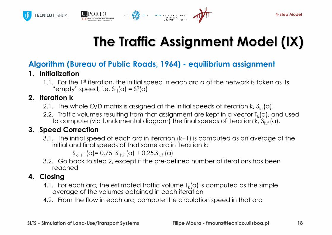
The Traffic Assignment Model (IX)Algorithm (Bureau of Public Roads, 1964) - equilibrium assignment1. Initialization

1.1. For the 1st iteration, the initial speed in each arc a of the network is taken as its “empty” speed, i.e. S1i(a) = S0(a)

2. Iteration k2.1. The whole O/D matrix is assigned at the initial speeds of iteration k, Sk,i(a). 2.2. Traffic volumes resulting from that assignment are kept in a vector Tk(a), and used

to compute (via fundamental diagram) the final speeds of iteration k, Sk,f (a).3. Speed Correction

3.1. The initial speed of each arc in iteration (k+1) is computed as an average of the initial and final speeds of that same arc in iteration k:

Sk+1,i (a)= 0.75. S k,i (a) + 0.25.Sk,f (a)3.2. Go back to step 2, except if the pre-defined number of iterations has been

reached4. Closing

4.1. For each arc, the estimated traffic volume Tk(a) is computed as the simple average of the volumes obtained in each iteration

4.2. From the flow in each arc, compute the circulation speed in that arc


4-Step Model

Uncertainty (I)


Source: Modelling Transport, Ortuzar and Willumsen

4-Step Model

Uncertainty (II)


Source: Petrik, O., Moura, F. M., Ghebrehiwot, Y., & Silva, J. (2012). Measuring uncertainty on the Portuguese high-speed railway demand forecast models. In Proceedings of 13th International Conference on Travel BehaviourResearch, Toronto.

4-Step Model

Uncertainty (III)


Uncertainty propagation through 4-step models

Source: Zhao, Y., & Kockelman, K. M. (2002). The propagation of uncertainty through travel demand models: an exploratory analysis. The Annals of regional science, 36(1), 145-163.

4-Step Model

General Criticism of the 4 Step Model (I)• The 4 step model faces serious criticisms to its capacity to

adequately represent contemporary mobility patterns, but it is still the most widely used

• As most usual criticisms are:– It does not include any possibility of representation of interdependencies

between trips of one person during the day or of his trips and those of other people in the same household

– It does not include any consideration of the choice of the hour for traveling

– In the 2nd step, the probabilistic choice of destinations from each origin is made based on accessibility costs for each of the zones, but those costs will be different for each mode, and this is the decision made on the 3rd

step. If we invert the order of these steps, the result is even more absurd, as we choose mode before choosing destination

– The choice of mode in the 3rd step is based on costs and times of each of the modes, but the impact of congestion is only know at the exit of the 4th

step, and this may change the results f the 3rd step


4-Step Model

General Criticism of the 4 Step Model (II)• For the two first criticisms the answer is activity based modeling (but still

with its own problems)• It is common practice today to merge the second and third steps in a

discrete choice of wide dimension (large number of alternatives), where each alternative is a combination of destination and mode to get thereØ Some pairs will not exist, as there is no connection by a given mode to a given

destinationØ The utility of each pair (destination, mode) includes positive utility components

(associated with the mass of the destination) and negative utility components (associated with accessibility conditions)

• The 4th step is run on the matrices (Origin / Destination / Mode) resulting from previous steps and an iterative procedure is applied, whereby the results of the 4th step are fed back into the input of the merged 2nd and 3rd steps for correction of speeds and thus of negative utilities.

• The iterative process stops when the differences of assigned volumes in the main arcs in successive iterations will be small enough


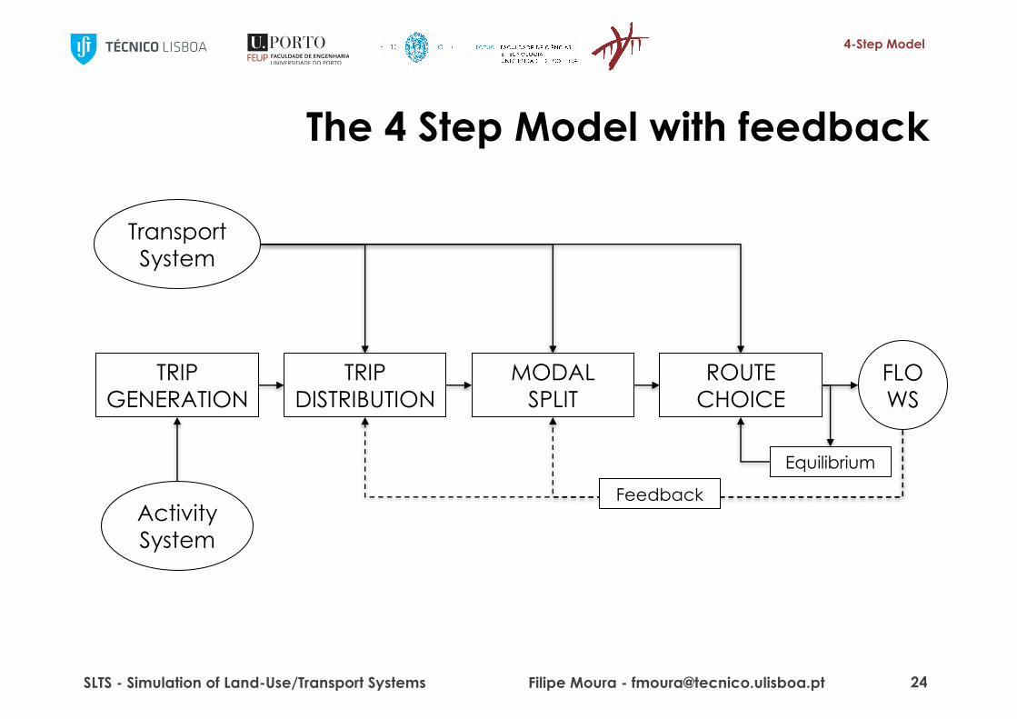
4-Step Model

The 4 Step Model with feedback


TRIP GENERATION

TRIP DISTRIBUTION

MODAL SPLIT

ROUTE CHOICE

FLOWS

Equilibrium

FeedbackActivity System

Transport System

4-Step Model

Bibliography• Ortuzar, Juan de Dios and Willumsen, Luis, Modelling Transport, 3rd

edition,, Wiley and Sons Ltd, 2001 – chapters 4, 5, 6 and 10

• Thomas, R, Traffic Assignment Techniques, ISBN 1856281663, Ashgate, 1991

• Bart Jourquin and Sabine Limbourg, Equilibrium Traffic Assignment on Large Virtual Networks: Implementation issues and limits for multi-modal freight Transport, EJTIR, 6, no. 3 (2006), pp. 205-228

• Joseph N. Prashker and Shlomo Bekhor, Some Observations on Stochastic User Equilibrium and System Optimum of Traffic Assignment, Transportation Research Part B 34 (2000), pp. 277-291


4 step model - ulisboa model theory of utility maximization: ... programs on travel demand. ......

Documents