4 new-patch-agggregation.pptx

Large-scale visual recognition Novel patch aggregation mechanisms

Florent Perronnin, XRCE Hervé Jégou, INRIA

CVPR tutorial on Large-Scale Visual Recognition June 16, 2012

Motivation

For large-scale visual recognition, we need image signatures which contain fine-grained information: •! in retrieval: the larger the dataset size, the higher the probability to find

another similar but irrelevant image to a given query •! in classification: the larger the number of other classes, the higher the

probability to find a class which is similar to any given class

BOV answer to the problem: increase visual vocabulary size ! see previous part on scaling visual vocabularies

How to increase amount of information without increasing the visual vocabulary size?

Motivation

BOV is only about counting the number of local descriptors assigned to each Voronoi region

Why not including other statistics?

http://www.cs.utexas.edu/~grauman/courses/fall2009/papers/bag_of_visual_words.pdf

Motivation


Why not including other statistics? For instance: •! mean of local descriptors


Motivation


Why not including other statistics? For instance: •! mean of local descriptors •! (co)variance of local descriptors


Outline

A first example: the VLAD

The Fisher Vector

Other higher-order representations

Example results


Given a codebook , e.g. learned with K-means, and a set of local descriptors :

•! ! assign:

•! "# compute:

•! concatenate vi’s + normalize

Jégou, Douze, Schmid and Pérez, “Aggregating local descriptors into a compact image representation”, CVPR’10.

µ 3

x

v1 v2 v3 v4

v5

µ1

µ 4

µ 2

µ 5

assign descriptors

compute x- µ i

vi=sum x- µ i for cell i


A graphical representation of



But in which sense is the VLAD optimal?

Could we add other (higher-order) statistics?

Outline

A first simple example: the VLAD

The Fisher Vector


Example results

The Fisher vector Score function

Given a likelihood function with parameters ", the score function of a given sample X is given by:

! Fixed-length vector whose dimensionality depends only on # parameters.

Intuition: direction in which the parameters " of the model should we modified to better fit the data.

F. Perronnin, H. Jégou, CVR tutorial on LSVRC, June 16, 2012.

The Fisher vector Fisher information matrix

Fisher information matrix (FIM) or negative Hessian:

Measure similarity between using the Fisher Kernel (FK):

! can be interpreted as a score whitening

As the FIM, is PSD, it can be decomposed as:

and the FK can be rewritten as a dot product between Fisher Vectors (FV):

Jaakkola and Haussler, “Exploiting generative models in discriminative classifiers”, NIPS’98.

The Fisher vector Application to images

is the set of T i.i.d. D-dim local descriptors (e.g. SIFT) extracted from an image:

! average pooling is a direct consequence of independence assumption

is a Gaussian Mixture Model (GMM) with parameters trained on a large set of local descriptors ! a probabilistic visual vocabulary

Perronnin and Dance, “Fisher kernels on visual categories for image categorization”, CVPR’07.

FV formulas:

The Fisher vector Relationship with the BOV

0.5

0.4 0.05

0.05


FV formulas: •! gradient wrt to w

!

! soft BOV

= soft-assignment of patch t to Gaussian i



0.5

0.4 0.05

0.05

•! gradient wrt to µ and # FV formulas: •! gradient wrt to w

!

! soft BOV


! compared to BOV, include higher-order statistics (up to order 2)

Let us denote: D = feature dim, N = # Gaussians •! BOV = N-dim •! FV = 2DN-dim



0.5

0.4 0.05

0.05

•! gradient wrt to µ and # FV formulas: •! gradient wrt to w

!

! soft BOV


! compared to BOV, include higher-order statistics (up to order 2)

!! FV much higher-dim than BOV for a given visual vocabulary size !! FV much faster to compute than BOV for a given feature dim



0.5

0.4 0.05

0.05

The Fisher vector Dimensionality reduction on local descriptors Perform PCA on local descriptors: ! uncorrelated features are more consistent with diagonal assumption of

covariance matrices in GMM ! FK performs whitening and enhances low-energy (possibly noisy) dimensions

The Fisher vector Dimensionality reduction on local descriptors Perform PCA on local descriptors: ! uncorrelated features are more consistent with diagonal assumption of

covariance matrices in GMM ! FK performs whitening and enhances low-energy (possibly noisy) dimensions

Jégou, Perronnin, Douze, Sánchez, Pérez and Schmid, “Aggregating local descriptors into compact codes”, TPAMI’11.

Results on INRIA Holidays

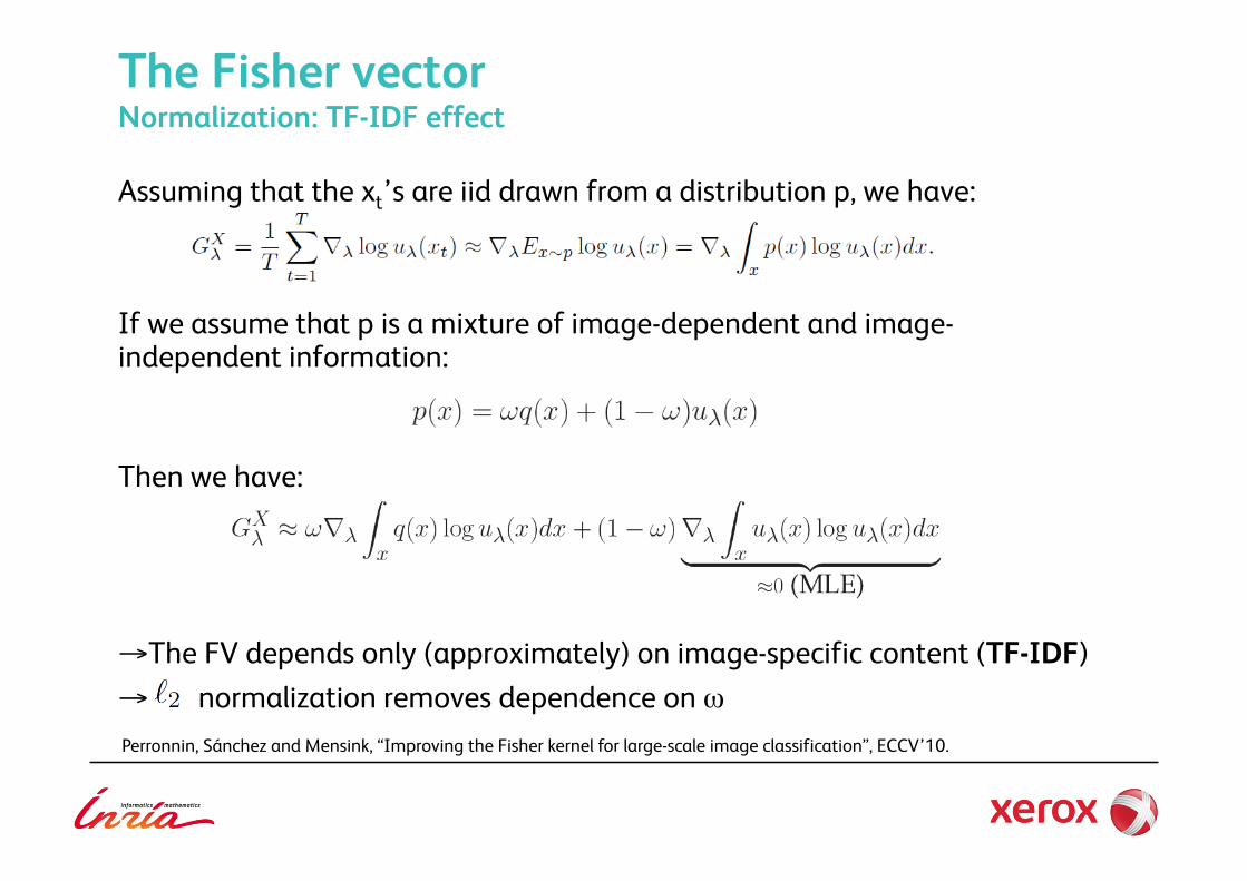
Assuming that the xt’s are iid drawn from a distribution p, we have:

If we assume that p is a mixture of image-dependent and image-independent information:

Then we have:

!!The FV depends only (approximately) on image-specific content (TF-IDF) !! normalization removes dependence on $

The Fisher vector Normalization: TF-IDF effect

Perronnin, Sánchez and Mensink, “Improving the Fisher kernel for large-scale image classification”, ECCV’10.

The Fisher vector Normalization: variance stabilization FVs can be (approximately) viewed as emissions of a compound Poisson: a sum of N iid random variables with N~Poisson. !! variance depends on mean

!! Variance stabilizing transforms of the form: (with %=0.5 by default)

can be used on the FV (or the VLAD).


Perronnin, Sánchez and Mensink, “Improving the Fisher kernel for large-scale image classification”, ECCV’10.

The Fisher vector Normalization: variance stabilization FVs can be (approximately) viewed as emissions of a compound Poisson: a sum of N iid random variables with N~Poisson. !! variance depends on mean

!! Variance stabilizing transforms of the form: (with %=0.5 by default)

can be used on the FV (or the VLAD).

! Reduce impact of bursty visual elements Jégou, Douze, Schmid, “On the burstiness of visual elements”, ICCV’09.


Outline


The Fisher Vector


Example results

But in which sense is the VLAD optimal?

Could we add other (higher-order) statistics?

Other higher-order representations Revisiting the VLAD


But in which sense is the VLAD optimal? ! The VLAD can be viewed as a non-probabilistic version of the FV: •! gradient with respect to mean only •! replace GMM clustering by k-means

!

Could we add other (higher-order) statistics? ! extension of the VLAD to include 2nd order statistics: VLAT Picard and Gosselin, “Improving image similarity with vectors of locally aggregated tensors”, ICIP ‘11.

Other higher-order representations Revisiting the VLAD

Other higher-order representations Super-Vector (SV) coding

is Lipschitz smooth if :

Given a codebook and a patch we have:

with

and (to be learned)

Zhou, Yu, Zhang and Huang, “Image classification using super-vector coding of local image descriptors”, ECCV’10.

Other higher-order representations Super-Vector (SV) coding

is Lipschitz smooth if :

Given a codebook and a patch we have:

with

Average pooling ! SV ! BOV + VLAD

Bound in Lipschitz smooth inequality provides argument for k-means.

Zhou, Yu, Zhang and Huang, “Image classification using super-vector coding of local image descriptors”, ECCV’10. See also: Ladick" and Torr, “Locally linear support vector machines”, ICML’11.

Outline


The Fisher Vector


Example results

Examples Retrieval Example on Holidays:

From: Jégou, Perronnin, Douze, Sánchez, Pérez and Schmid, “Aggregating local descriptors into compact codes”, TPAMI’11.


!! second order statistics are not essential for retrieval



!! second order statistics are not essential for retrieval !! even for the same feature dim, the FV/VLAD can beat the BOV



!! second order statistics are not essential for retrieval !! even for the same feature dim, the FV/VLAD can beat the BOV !! soft assignment + whitening of FV helps when number of Gaussians &



!! second order statistics are not essential for retrieval !! even for the same feature dim, the FV/VLAD can beat the BOV !! soft assignment + whitening of FV helps when number of Gaussians & !! after dim-reduction however, the FV and VLAD perform similarly


Examples Classification Example on PASCAL VOC 2007:

From: Chatfield, Lempitsky, Vedaldi and Zisserman, “The devil is in the details: an evaluation of recent feature encoding methods”, BMVC’11.

Feature dim mAP

VQ 25K 55.30

KCB 25K 56.26

LLC 25K 57.27

SV 41K 58.16

FV 132K 61.69



! FV outperforms BOV-based techniques including: •! VQ: plain vanilla BOV •! KCB: BOV with soft assignment •! LLC: BOV with sparse coding

Feature dim mAP

VQ 25K 55.30

KCB 25K 56.26

LLC 25K 57.27

SV 41K 58.16

FV 132K 61.69



! FV outperforms BOV-based techniques including: •! VQ: plain vanilla BOV •! KCB: BOV with soft assignment •! LLC: BOV with sparse coding

! including 2nd order information is important for classification

Feature dim mAP

VQ 25K 55.30

KCB 25K 56.26

LLC 25K 57.27

SV 41K 58.16

FV 132K 61.69

Packages

The INRIA package: http://lear.inrialpes.fr/src/inria_fisher/

The Oxford package (soon to be released): http://www.robots.ox.ac.uk/~vgg/research/encoding_eval/

Questions?

4 new-patch-agggregation.pptx

Engineering

number of local descriptors

set of local descriptors

fisher vector score

simple example

higherorder statistics

assign descriptors compute

fisher kernel fk

largescale visual recognition