4

fl TN NO: N-1628LA

TITLE: WIND-INDUCED STEADY LOADS ON SHIPS

i 7nC

AUTHOR: R- Owens and P. ealo 7 1982T

DATE: April 1982 H

SPONSOR: Naval Facilities Engineering Command

I !J PROGRAM NO: YF59.556.091.01.403

>" NAVAL CIVIL ENGINEERING LABORATORYPORT HUENEME, CALIFORNIA 93043Approved for public release distribution unlimited.

82 10 07 0111

oI C. -o

EE E

L z

C C

~~ aiZ Z;

NN~~~~ c.c; ~RLm

A t L 0

UnclassifiedSECURITY CLASSIFICATION 0' T.15 -AGE rWhon n.t. F^-,.dj

REPORT DOCUMENTATION PAGE BFR OPEIGFRIREPORT NUUBFN 12. GOVT ACCESSION NO. 1. RECIPIENT'S CATALOG NUMBER

TN -1628 terv ~ ____

4. TITLE ford Sub.e) S TYPE or REPORT A PERIOD COVERED

WIND-INDUCED STEADY LOADS ON SHIPS Not final; Oct 1980 - Jun 19816 PERFORMING ORG. REPORT NUMBER

7 AUTHOR(.) 6, CONTACT OR GRANT NUMUERfsJ

R. Owens and P. Palo

9. PERF~ORMING ORGANIZATION NAME AND ADDRESS to P ROGRAM ELEMENT. PROJECT, TASKAREA & WORK UN IT N.UMBERS

NAVAL CIVIL ENGINEERING LABORATORY 62759N;Port Hueneme, California 93043 YF59.556.091.01.403

II. CONTROLLING OFFICE NAME AND ADDRESS 12, REPORT DATE

Naval Facilities Engineering Command April 1982Alexandria, Virginia 22332 55NMBR0

14 MONITORING AGENCY NAME & AODRESSOJl d,ii,.n o.. C.,n,,.,fl4n* Oil--.) IS SECURITY CLASS. (of 1k,. -Volt?)

UnclassifiediS.. OECLASSIFICATION DOWNGR.AOING

SCHEDULE

16, DISTRIBUTION STATEMENT N1 l N. H-P-,Ij

Approved for public release; distribution unlimited.

17. DISTRIBUTION STATEMENT (of Ithe abv,,.t P,,d ,n Block 20. -0 dill.,onI from Raporf)

IS. SUPPLEMENTARY NOTES

19 KEY WORDS (Corttiriu. act wdol8 SI re rtam ol#* V d idirflfli b, black numbel)

Wind forces, moorings, ships.

20 A3*Z3 ,ACT (Cor.inue ort *eeills side it necessary ocid idvitily br block number)

Methods are presented for predicting the lateral and longitudinal steady wind dragforces and yaw moment versus incident wind angle for various ship types. These methodswere developed based on experimental model data for 31 ships compiled from six indepen-dent tests. Except for hull-dominated ships, which are considered separately, the longitudinalwind drag force is computed using a constant headwind coefficient that has an accuracy of

(continued)

DD , JOAn7 1473 EDITION OF I NOV 61 IS OBSOLETE UnclassifiedSECURITY CLASSIFICATION OF THIS PAGE (When Data £,,U.,ad)

UnclassifiedSECUNITY CLASSIFICATIOt O

r TIS PAGE(Wbho D es Et..Ir.d)

20. Continued

12%. This coefficient can be modified depending on the ship type and above deck features.Over the remainder of the incident wind directions the coefficient is based on curve fits tothe data. The lateral force coefficient is also derived from a curve fitted to the data and isbased on a peak value with a 10% deviation; the coefficient is dependent on mean heightsand projected areas of the hull and superstructure. Determination of the rccommendedmoment response is based on an inspection and interpolation of existing experimental data.Recommendations from other investigations are also presented for comparison, and asample problem is included.

Library Card

---- -valCiMt~ngneerm'g 1t-t'WIND-INDUCED STEADY LOADS ON SHIPS, by IL Owens andP. PaloTN-1628 55 pp illus Aprl 1982 Unclassified

1. Wind drag force 2. Yaw moment response I. YF59.556.091.01.403

Methods are presented for predicting the lateral and longitudinal steady wind drag forcesand yaw moment versus incident wind angle for various ship types. These methods were developedbased on experimental model data for 31 ships compiled from six independent tests. Except forhull-dominated ships, which are considered separately, the longitudinal wipd drag force is com-puted using a constant headwind coefficient that has an accuracy of 12%. This coefficient can bemodified depending on the ship type and above deck features. Over the remainder of the incidentwind directions the coefficient is based on curve fits to the data. The lateral force coefficient isalso derived from a curve fitted to the data ad is based on a peak value with a 10% deviation; thecoefficient is dependent on mean heights and projected areas of the hull and Superstructure.Determination of the recommended moment response is based on an inspection and interpolationof existing experimental data. Recommendations from other investigations are also presentedfor comparison, and a sample problem is included.

UnclassifiedSECURIY CLASSIICATION OF THiS PAGI[ 'RfM Doa s

CONTENTS

Page

INTRODUCTION ... . . . . . . . . . . . . . . . . . . . . . . . . I

EXPERIMENTAL DATA .. ........... .............. 2

SUMMARY OF WIND FORCE EQUATIONS. ..... .............. 3

Lateral Wind Force. .... ................... 3Longitudinal Wind Force .. .... ................ 4Wind Moment. .. ............ ............. 7

DEVELOPMENT OF PROCEDURE ....................

Wind Gradient. .. ............ ........... 7Lateral Wind Force. ............. ....................... 8Lateral Wind Shape Function. .. ......... .. .... 10Longitudinal Wind Force. .. ............. ..... 11Wind Yaw Moment .. ... .................... 13

ATYPICAL SHIP TYPES. .... .................... 15

DISCUSSION OF RECOMMENDED PROCEDURES. .. .............. 16

Comparisons to Experimental Data .. .............. 16

Comparison to Other Investigators. .. ............. 17

CONCLUSIONS AND RECOMMENDATIONS .. ............. .... 18

ACKNOWLEDGMENT .. .... .................. .... 18

REFERENCES .. .... ................... ..... 18

NOMENCLATURE .. ... ................... ..... 21

APPENDIX -Sample Problem. ... .................. 47

)IN Itd~ -

i LSpeONo

V

F"I

YI

bow __________ _____stern -

x

NONDIMENSIONAL COEFFICIENTS

CX=longudmal force coefficienz

CY . lateral force coefficient

CN - yaw momcnt coefficient

8 < 00 o

Posi~ive Wind Load Conventionsand Coordinate System

Vi

INTRODUCTION

One major source of error in the design of mooring systems for

large ships has been the lack of accurate knowledge of wind loads. Many

of the present methods for calculating these loads are unreliable or

cumbersome to use. One method, proposed primarily for its simplicity,

is presented in the chapter 7 revision of the NAVFAC Design Manual DM-26

(Ref 1). This method involves three curves that are useG for the lateral,

longitudinal, and moment loads for all ships. However, experimental

data have shown this approach to be too approximate for general appli-

cation.

The purpose of this document is to describe an improved method for

computing accurately and easily the wind drag forces, by taking gross

individual ship characteristics into account. Results of this investi-

gation are applicable primarily to "typical" ships, although some of the

31 models used were not typical. Even so, an effort was made to present

trends and recommendations for "atypical" ships by using their collected

responses to better define the wind load characteristics of unique ships

and to amplify coefficient trends for the more typical ships.

In many cases accurate data regarding projected and other surface

areas of the models are lacking. For this reason, along with the fact

that scale model behavior is often not completely representative of full

scale ship behavior (surface roughness, railings, etc.), the accuracy of

the experimental results is not above question. Care was taken to

establish the reliability and accuracy of all experimental results by

comparing projected model areas to a variety of sources and by comparing

results of independent tests for similar ships.

Because of the complex superstructure geometry on most ships, the

lateral and longitudinal wind forces can be calculated more directly

than the moment. The emphasis of this note is, therefore, placed on the

accurate determination of these two forces, while the moment response is

only observed for trends. The effect of the naturally occurring wind

gradient has also been incorporated into this analysis, especially for

the case of the lateral wind force, where the projected ship area is

greatest.

This analysis was undertaken because of the concern for reliable

ship load files (for wind and curreut loads) expressed in Reference 2

and deals only with the wind load aspect. The design procedures devel-

oped here are particularly useful for mooring analysis problems in

protected harbors, where wave and current loads are usually small. This

work was performed as part of the effort on Mooring Systems Frediction

Techniques within the Ocean Facilities Engineering Exploratory Develop-

ment Program, sponsored by t'- Naval Facilities Engineering Command.

EXPERIMENTAL DATA

The experimental data used in this investigation were taken from

six independent sources (Refs 3 through 8); data on 31 ship models were

used from the available 40 models. The data not used were those consid-

ered to be from unconventional models or those lacking information ill

some respect. Also, only data on 2 ship models were used from Reference 7

because the data are considered by many to be too conservative. Of the

31 models used: 18 were tankers and cargo ships, including 4 center

island tankers; 3, aircraft carriers; 2, cruisers; 1, a destroyer, which

was independently tested by two sources; 2, passenger liners; and the

remaining 5, general class.

Data from 19 of these 31 models were used for the CX coefficient

determination and 13 for the C coefficient determination because not

all sources used a wind gradient in the experiment, and because the main

concern of this investigation was with tankers and cargo ships; there

were less data on warships. From these data, a more reliable method for

calculating wind loads than that given by the three reference curves

presented in Reference 1 and illustrated in Figure 1 was developed

2

Approximate silhouettes for some of these ships are presented in Figure 2

to allow the reader to associate the recommendations from this report

with the various ship types.

SUMMARY OF WIND FORCE EQUATIONS

Equations for the lateral and longitudinal forces versus incident

wind angle are presented in this section. Derivations and a discussion

are presented in later sections. It should be stated that these forces

are actually dependent on Reynolds Number, which is assiuaed for typical

ships to be large enough to allow for constant coefficients. The general

equation for these forces can be expressed as follows:

1 2F - A C f(O) (1 )

where;

F = wind force, FX or Fy, or yaw moment, N

p density of air

V relative wind velocity with respect to ship

A = projected ship area, Ax (used for FX) ; or Ay (used for F y);or Ay L used for N, L ship length

C Z dimensiouiless wind drag coefficient, C , Cy, or C N

f(O) = normalized shape function dependent on incident wind angle (0)

Lateral Wind Force

The following results have been obtained for the lateral wind drag

coefficient (Cy) by sumaiing forces obtained for the hull and superstruc-

ture:

3, .,

I-.

where the [(R) As + (\ ) (2)

cy A, , (2)

where the terms (Vs/VR) and VH /VR) are the average wind velocities over

the superstructure and the hull, respectively, taken from a normalized

wind gradient curve presented in Figure 3. CC was determined from the

available experimental data and was calculated to be:

C YC 0.92 t 0.1

The following recommended normalized shape function was fitted to the

available data:

f(O)= sn e - sin (50)/201jLS/2

(3)f (0) 1 - 1/20

This function is illustrated in Figure 4.

Longitudinal Wind Force

The longitudinal wind force calculations are not as straightforward

as the lateral force calculations. Both the coefficient and shape func-

tion vary according to ship type and characteristics.

Selection of Longitudinal Force Coefficient (Cx). In gtneral,

vessels are classified as either hull dominated, (such as aircraft

carriers and passenger liners) or normal (such as warships, tankers).

Second, due to possible asymnetry of the superstructure relative to

midships, separate coefficients are used for headwind and tailwind

loadings, designated as CXB and C XS respectively.

For hull dominated vessels, the following is recommended:

C = C = 0.40

4

For all remaining types of ships, except for specific deviations,

the following are recommended:

C = 0.70

C = 0.60

Deviations to these general coefficients are listed below. First,

for center island tankers only, an increased headwind coefficient is

recommended:

C = 0.80

For ships with an excessive amount of superstructure, such as des-

troyers and cruisers:

C = 0.80xs

A universal adjustment of 0.08 is also recommended for all cargo

ships and Latikers with cluttered decks (i.e., masts, booms, piping, aidi

other substantial obstructions). This would apply to both CXB and C S

Selection of the Longitudinal Shape Function (f(6)). As with the

longitudinal coefficient, two distinct longitudinal shape functions arc

recommended that differ over the headwiad and tailwind regions. These

regions are separated by the incident wind angle that produces no net

longitudin3l force, designated 0Z for zero crossing. Selection of 0Z is

determined by the mean superstructure location relative to midships (MS):

Just forward of MS: 0Z = 80 degrees

oil MS: 0Z = 90 degrees

aft of MS: 0 = 100 degrees

Hull dominated: 0Z = 120 degrees

Generally, 0Z - 100 degrees seems typical for many ships, including

center island tankers, while 0 -110 degrees is recommended for warships.z

5

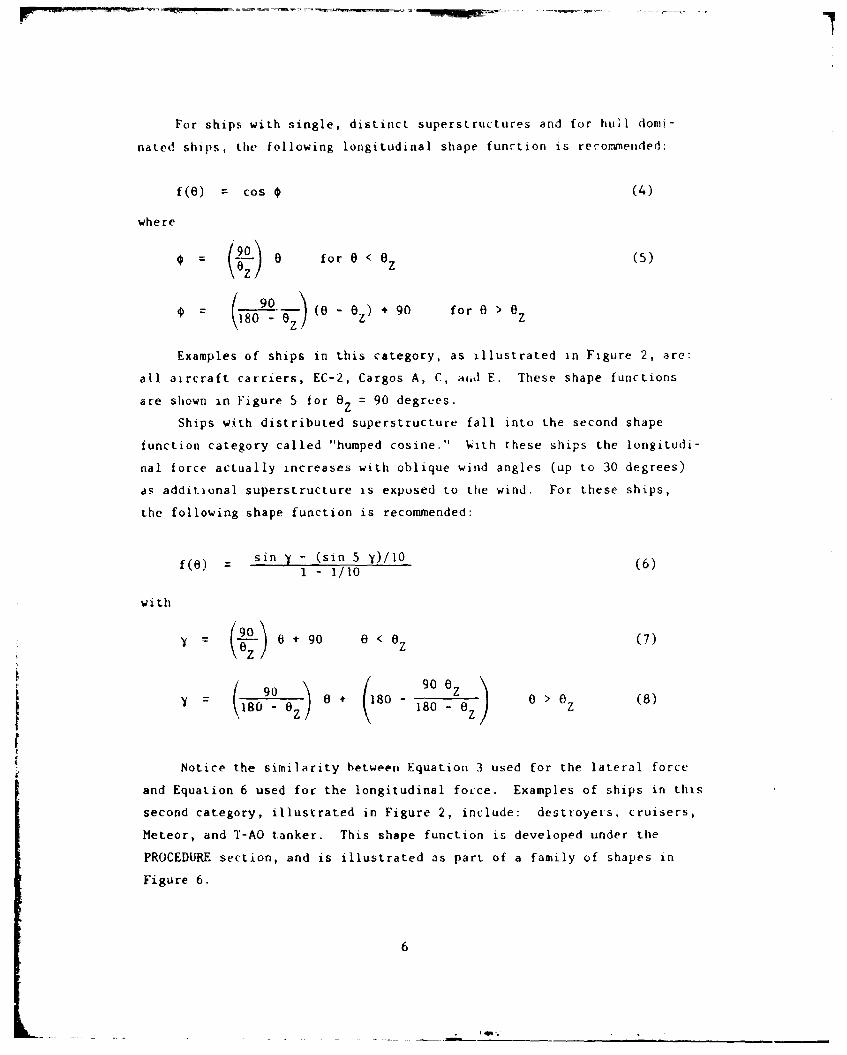
For ships with single, distinct superstructures and for hull doni-

nated ships, the following longitudinal shape function is recommended:

f(0) cos * (4)

where

* (- Z) 0 for e < 0O (5)

= 8090 (0 - 0Z) + 90 for 0 > 6Z

Examples of ships in this category, as illustrated in Figure 2, are:

all aircraft carriers, EC-2, Cargos A, C, and E. These shape functions

are shown in Figure 5 for 6z = 90 degrees.

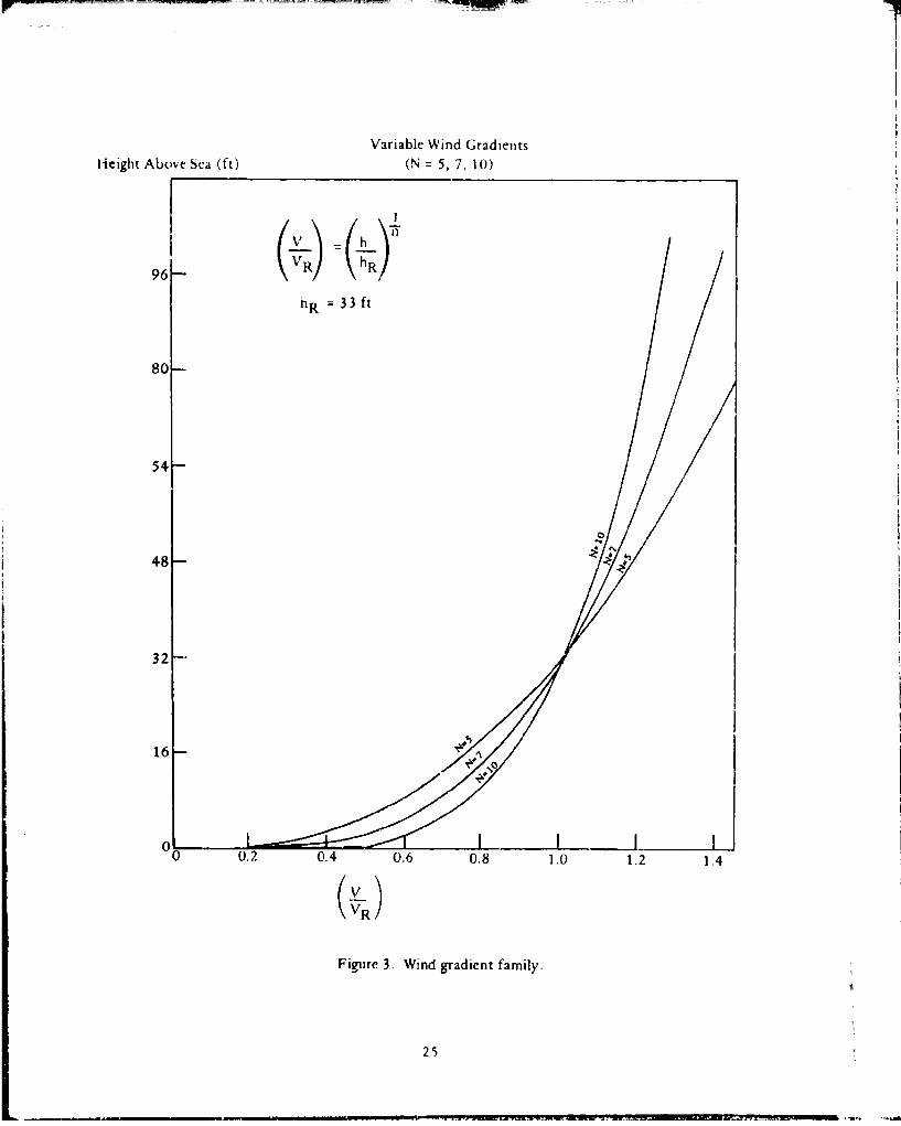
Ships with distributed superstructure fall into the second shape

function category called "humped cosine." With these ships the longitudi-

nal force actually increases with oblique wind angles (up to 30 degrees)

as additional superstructure is exposed to the wind. For these ships,

the following shape function is recommended:

f(0) sin " - (sin 5 y)/10 (6)

1 - 1/10

with

(9 ) 6 g o < o' (7)

: a + 80 • 0 > 0 (8)

(80 - 0( 180- z z

Notice the similarity between Equation 3 used for the lateral force

and Equation 6 used for the longitudinal focCe. Examples of ships in this

second category, illustrated in Figure 2, include: destroyers, cruisers,

Meteor, and T-AO tanker. This shape function is developed under the

PROCEDURE section, and is illustrated as part of a family of shapes in

Figure 6.

6

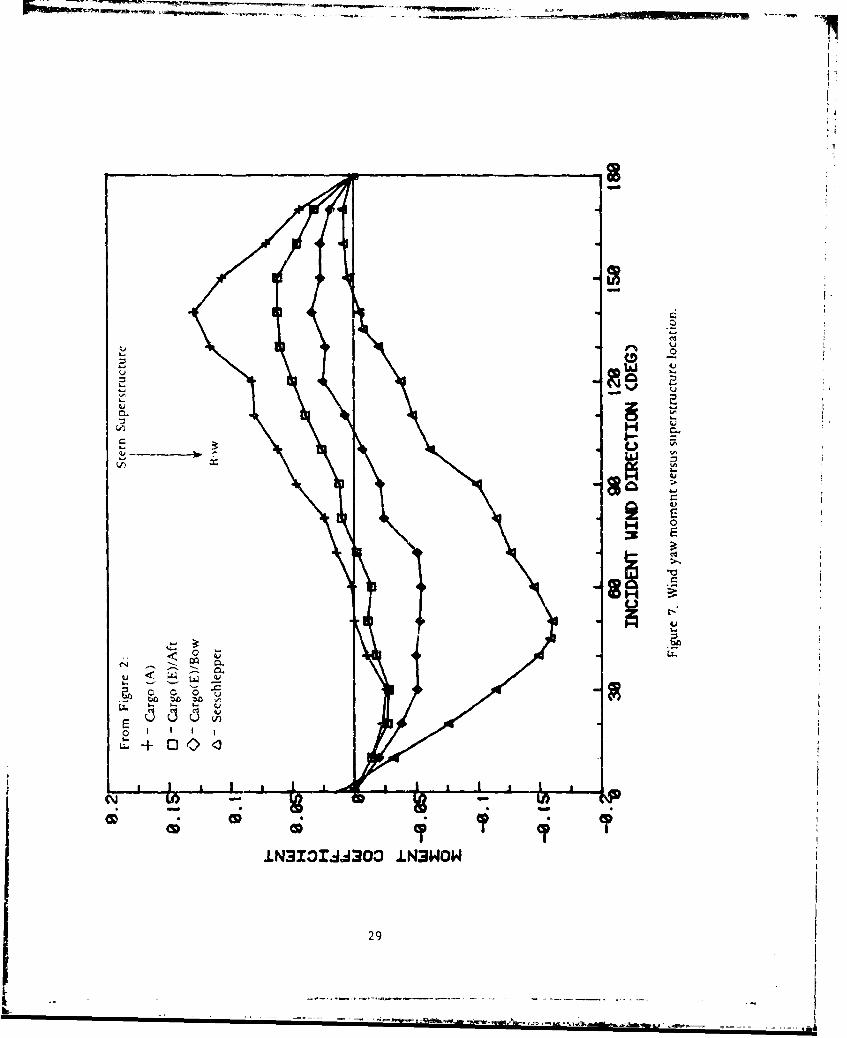
Wind Moment

For the general moment response tendencies of a ship, refer to

Figure 7. More specific moment coefficient curves are presented in

Figures 8 through 14 for the various ship types considered. More

details concerning the moment response are provided in the DEVELOPMENT

OF PROCEDURE section.

DEVELOPMENT OF PROCEDURE

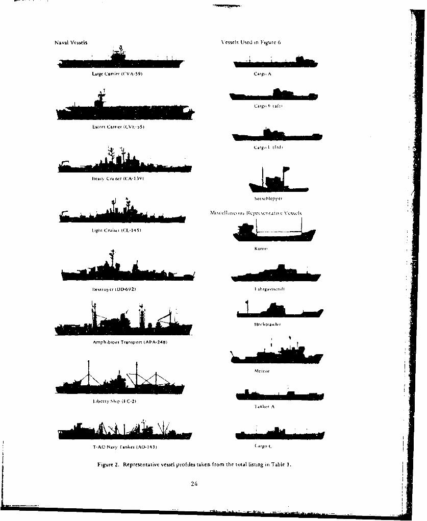
Wind Gradient

The two major factors that directed the approach of this investiga-

tion were: quantifying the effects of the natiral wind gradient over

the ship profile, and allowing for more individualized shape functions

based on vessel characteristics.

The wind gradient is obtained from the following equation (Ref 9);

IVR ~ (9)

where,

V

VI = normalized wind velocity at height (h)

h = height above free strface

hR = constant reference ieight

n = arbitrary exponent

For the pirposes of this report, the reference height (hR) is taken as

33 feet (10 meters) above the mean sea surface, and the exponent (n) is

assumed to be 7. It was determined that the value of n is not critical,

since no significant difference wis observed in the calculated wind drag

7

IL

forces when n was varied from 5 to 10; the value of n = 7 is chosen

primarily because it is the value most commonly used for this type of

application (Ref 10).

In dealing with the wind gradient, the hull and superstructure of

each vessel were considered separately. This proved effective for the

Cy coefficient, but no consistent results were obtained for the CX

coefficient. For this reason, the longitudinal wind load determination

is not as straightforward as the lateral wind load determination.

Lateral Wind Force

From Equation I

FC (10)YM 1 2~PV Ay,

Where C is the experimentally measured value cf the lateral wind drag

coefficient at an incident wind angle of 90 degrees. By separating the

total lateral force on a vessel into hall and superstructure components,

a lateral drag coefficient (Cyc) can be calculated. In this manner the

general equation for Fy, given by

F 1 V2 f(6) (11)ry = Ay cy

can be written

F S = ( AS + VH A) Cy f(8) (12)

where subscripts S and H refer to the superstructure and hull, respectively,

ard V denotes the mean wind velocity over each. Use of a constant drag

coefficient (Cyc) is considered valid because the hull arid superstructure

both appear as bluff bodies for lateral incident winds. Multiplying and

dividing by the relative velocity (VR) at 33 feet gives:

V2(V AS -5 A Cyc f(0) (13)

y AsR

' ' ' , n n n- , , i ...i~ i ' ' + . ... +"+ "" i 'i - 1 ........ ,

I

I-

From which

Cy F / I [)\V As + AH] f () (14)

( /R2 - 2where the values for (VH/VR) and (Vs/VH) are taken from the wind gradient

curve with n = 7 (Figure 3), and are the values that correspond to the

centers of area of the portions of the gradient curve that lie between

the height ranges of the hull and superstructure of the ship. Values of

C yc for the experimental values presented in terms of Equation 10 were

determined by taking the ratio of Equation 10 to Equation 14:

CyM Cyc = A S + (7, AH Ay (15)

Such that

Cyc (Cy)(AY) AS * (V AH] (16)

Representative C values were determined using data from 17 of the

31 ship models, and estimated wind gradients from the tests when reported.

Four of the C values for these 17 representative ship models were dis-

carded through comparisons to similar ship types and were attributed to

questionable or incomplete data concerning the gradient or projected

ship areas. A mean value was then determined from the remaining 13

models, yielding

i C =0.92 ±0.1Yc

This calculated value is consistent with an expected value of just

less than 1, based on drag measurements of flat plates that yield coeffi-

cients of 1.1 to 1.2 (Ref 11), and the fact that the hull and super-

structure are slightly streamlined in shape compared to a plate.

I19i

With the value of C constant at 0.92, Equation 16 becomes

YC

S0.92 1 y

o0.92 As ( t (17)

And using this peak coefficient value:

Cy(6) y f(0) ()

Lateral Wind Shape Function

The shape function, f(6), versus incident angle was determined by

transforming a normal siiie wave into a more flat-topped sine wave, which

was more characteristic of the lateral wind load coefficient. plots for

most of the 31 model ships analyzed. This transfigured shape function

is a result of the sumL,;tion of the standard sine wave with a sine wave

of period 1/5 the size (figure 15). The expressiun of this trial

shape functioa (C) is

f'(0) = sin 0 + M sin 56 where 0 degrees _ 0 < 180 degrees (i9)

Substituting for 0:

(A) at e = 90 degrees, f'(90) = 1 + M

(B) at 0 = 72 degrees, f'(72) = 0.95

Setting f'(90) = f'(72) to get the flat top, and solving for M

0.95 = 1 + M; M = -0.05

Substituting this coefficient into the function,

f'(0) sin 0 - (sin 50)/20 (20)

10

..

This trial shape function is now normalized as

f(6) = [sir, 6 - (sin 50)120]1(1 - 1/20) (21)

The final equation for the lateral wind drag force coefficient then becomes

Cy() Z {jsin 0 - (sin 56)/201/(1 - 1/20)} (22)

Equation 21 gives the standard form for the shape function for both the

lateral and longitudinal forces; changes in the constant (i.e., 20) and

argument of the sine allow use of the same basic equation for a pro-

gression of shape functions.

Longitudinal Wind Force

As previously stated, the separation method used for the lateral

coefficient (Cy) was not successful for the longitudinal coefficient

(CX) which assumed a hull coefficient of 0.4 based on the experimental

data for hull dominated vessels. An alternative inspection method wasused instead. The headwind coefficients of 19 of the model ships were

analyzed, and it was found that ships with cluttered decks have headwind

coefficients consistently higher than comparable ships with cleaner(trim) decks. Center islano tankers were found to have headwind coeffi-

cients from 15% to 25% higher than single superstructure vessels, depending

on trim or cluttered deck conditions.The measured headwind coefficients of the 19 models were then

adjusted, if necessary, according to the observations above, and a meat.

headwind coefficient of CXB = 0.70 ± 0.06 was obtained, except for hull

dominated ships (aircraft carriers) where the headwind coefficient

obtained was CXB 0.40. The tailwind coefficients for these 19 shipmodels were also analyzed; it was found that: Single (simple) superstruc-

ture vessels generally have a tailwind coefficient C -0.60; single

superstructure cluttered (piping, masts, etc.) vessels and hull dominated

vessels have CSL CX8; center island tankers have CXS 3/4CXB

and distributed superstructure vessels (cruisers and destroyers) have

XS 1.1 CXB.

11

-

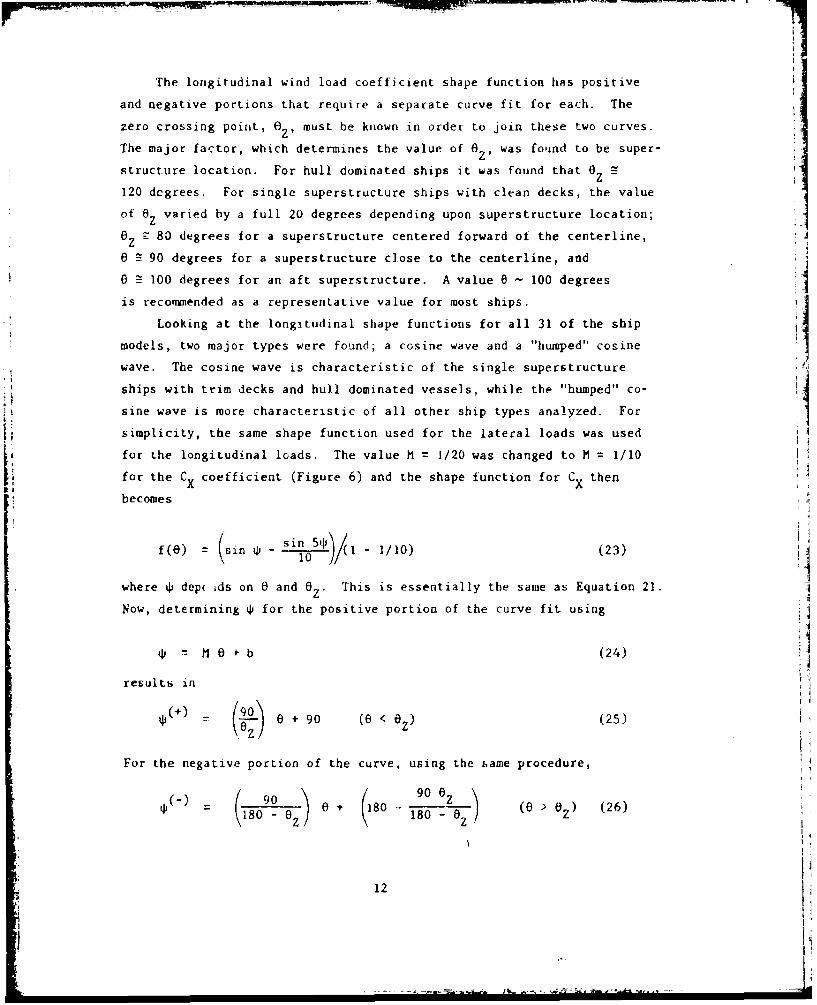
The longitudinal wind load coefficient shape function has positive

and negative portions that require a separate curve fit for each. The

zero crossing point, E, must be known in order to join these two curves.

The major factor, which determines the value of 0., was found to be super-

structure location. For hull dominated ships it was found that 0Z

120 degrees. For single superstructure ships with clean decks, the value

of 8Z varied by a full 20 degrees depending upon superstructure location;

8 Z 80 degrees for a superstructure centered forward of the centerline,

o 90 degrees for a superstructure close to the centerline, and

0 100 degrees for an aft superstructure. A value 8 - 100 degrees

is recommended as a representative value for most ships.

Looking at the longitudinal shape functions for all 31 of the ship

models, two major types were found; a cosine wave and a "humped" cosine

wave. The cosine wave is characteristic of the single superstructure

ships with trim decks and hu).l dominated vessels, while the "humped" co-

sine wave is more characteristic of all other ship types analyzed. For

simplicity, the same shape function used for the lateral loads was used

for the longitudinal loads. The value M = 1/20 was changed to M = 1/10

for the C coefficient (Figure 6) and the shape function for C then

becomes

f(e) ( sin tP - s / I - 1/10) (23)

where t4 dep(.ds on ( and 8 . This is essentially the same as Equation 21.

Now, determining tP for the positive portion of the curve fit using

4i M 0 *b (24)

results in

90-) 0 + 9 ( < z) (25)

For the negative portion of the curve, using the same procedure,

(-1 09o __9_0_0_z_80 __8

(- =80 * 180 Z (0 > 0,) (26)

12

Ii

so that

Cf ( 4 from Equation 25, (0 < 0) (27)

CX = C f 4- $- from Equation 26, (E > 0 . (28)x xs z.

These apply only to humped cosine curve types, while the shape functions

for the straight cosine curve shape are simply

f(to) = cos '4 (29)

= O) (0 < Z) (30)

(,() - (i89 )o (- 09 + 90 (0 > a (31)

Wind Yaw Moment

The yaw moment response (CN) is mnre difficult to predict than the

C and C responses because of the difficulties of accurately determiningx Ythe moment arms and interference effects of the superstructure and other

topside features that significantly add to the wind drag on each ship,

and because of a pronounced sensitivity to freeboard in many ships.

Hence, no curve fit was attempted, and all findings are based entirely

upon the observed moment coefficient curve of each model. Generalizations

concerning the moment response with respect to superstructure location

and apparent trends for the ship types covered are presented below.

The location of the superstructure seems to be the best indicator

of a ship's moment response. According to the conventions of this report,

as the main superstructure of a vessel progresses from stern to bow, the

moment tends from a positive to a negative orientation, as shown in

Figure 7. Similar to the definition of the C coefficient, the value of

6Z is the incident wind angle at which the CN coefficient crosses the

13

axis, changing from a negative to a positive moment (by the conventions

established in this report). Based on the experimental data used,

the following values of 6 and magnitude ratios of negative to

positive moment are given for the yaw moment coefficient curves of tle

model ship types analyzed.

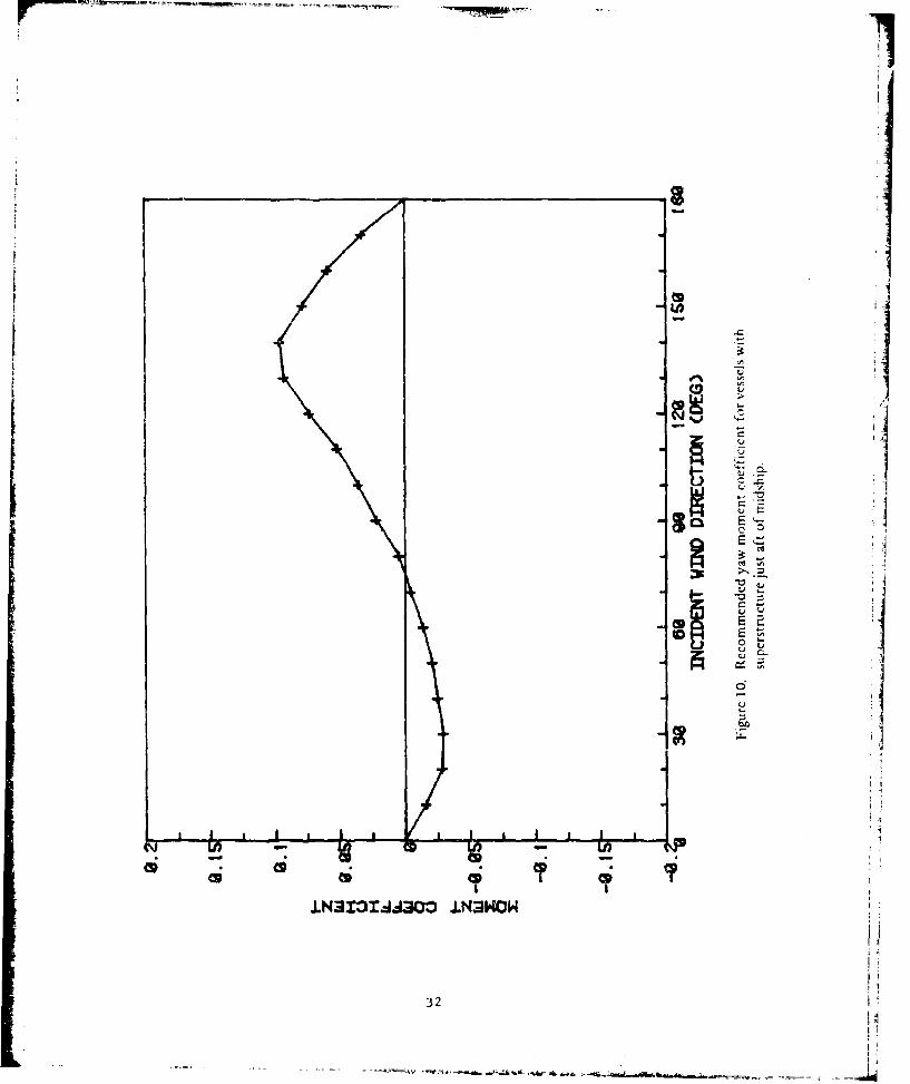
1. Single superstructure ships, grouped by location:

a. Stern

Trim - 0 60 degrees; 1:3Cluttered - 8 80 degrees; 1:2

b. Between stern and center

0Z z 80 degrees; 1:3

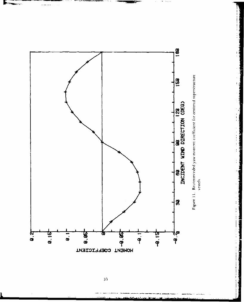
c. Center

Z 90 degrees; 1:1

d. Between center and bow J0Z 105 degrees; 1:1

2. Center Island Tankers: ATrim - 0 85 degrees; 1:2

Cluttered - 0 85 degrees -90 degrees; 1:1

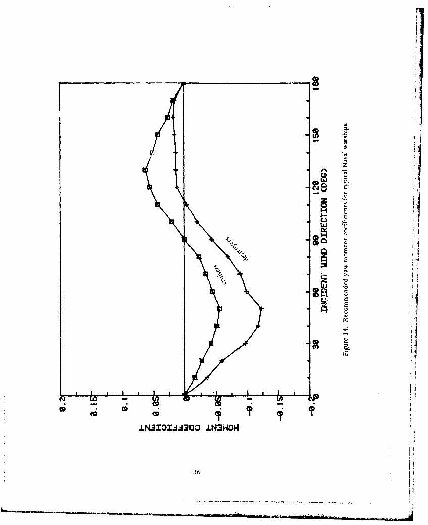
3. Distributed superstructure ships:

Cruisers

Oz L 90 degrees -100 degrees; 1:1

Destroyers

9 -510 degrees; -10dges4. Hull dominated ships: 1

Aircraft carriers. 0Z = 90 degrees - 100 degrees; 1:1

Passenger liners

0Z = 100 degrees; 2:1

Although useful, the above information is limited because the

magnitude ratios are strictly relative, with no reference coefficient

values given. The magnitude of the moment coefficient curve is dependent

14

on the size of projected superstructure and hull areas and the moment

arms through w'hich they act. Therefore, since no approximation for the

actual magnitudes of the moment ccefficient is given, example moment

curves have been provided for all ship types dealt with in this analvsis.

These curves are presented in Figures 8 through 14, representing the best

estimates (averages) attainable from the experimental model data used.

ATYPICAL SHIP TYPES

The methods presented in this report for calculating wind drag

coefficient curves are primarily geared toward tankers and cargo ships,

since these comprised the majority of the ship models investigated.

EVci, so, these same methods proved adequate for the warships that were

present in the experimental model data used. There are, however, several

uncharacteristic design features which create atypical ship type5 not

entirely compatible with the suggested methods of this report. One Fuch

atypical ship is the Kumo, which possesses an aft superstructure somewhat

larger than norma] with respect to the overall length of the ship and an

extremely prominent forecastle. Collectively, these two uncharacteristic

features cause a considerable increase in the headwind coefficient (C x)

for the CX wind load response to a value near 1.0, and an increase in the

peak Cy coefficient to a value between 0.90 - 1.0 in magnitude. The

moment response (CN) is essentially unaffected, with e z 60 degrees and

a magnitude ratio of 1:3 for the negative to positive moment orientation.

Other atypical ship types, at least for the purposes of this report,

are the smaller auxiliary and research vessels such as the METEOR. These

vessels have a distributed upper deck layout that causes them to behave

very much like a destroyer in their wind load responses.

All other atypical ships (submarines, catamarans, hydrofoils, etc.)

were not investigated in this study, so the use of the design methods

presented in this report for determining the loads on such ships is not

recommended.

15

DISCUSSION OF RECOMMENDED PROCEDURES

To provide the reade. with a better perspective regarding the

accurdcy and praticality of the methods recommended here, comparisons

will be made to representative experimental results and recommendations

from earlier investigators.

Comparisons to Experimental Data

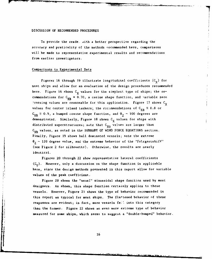
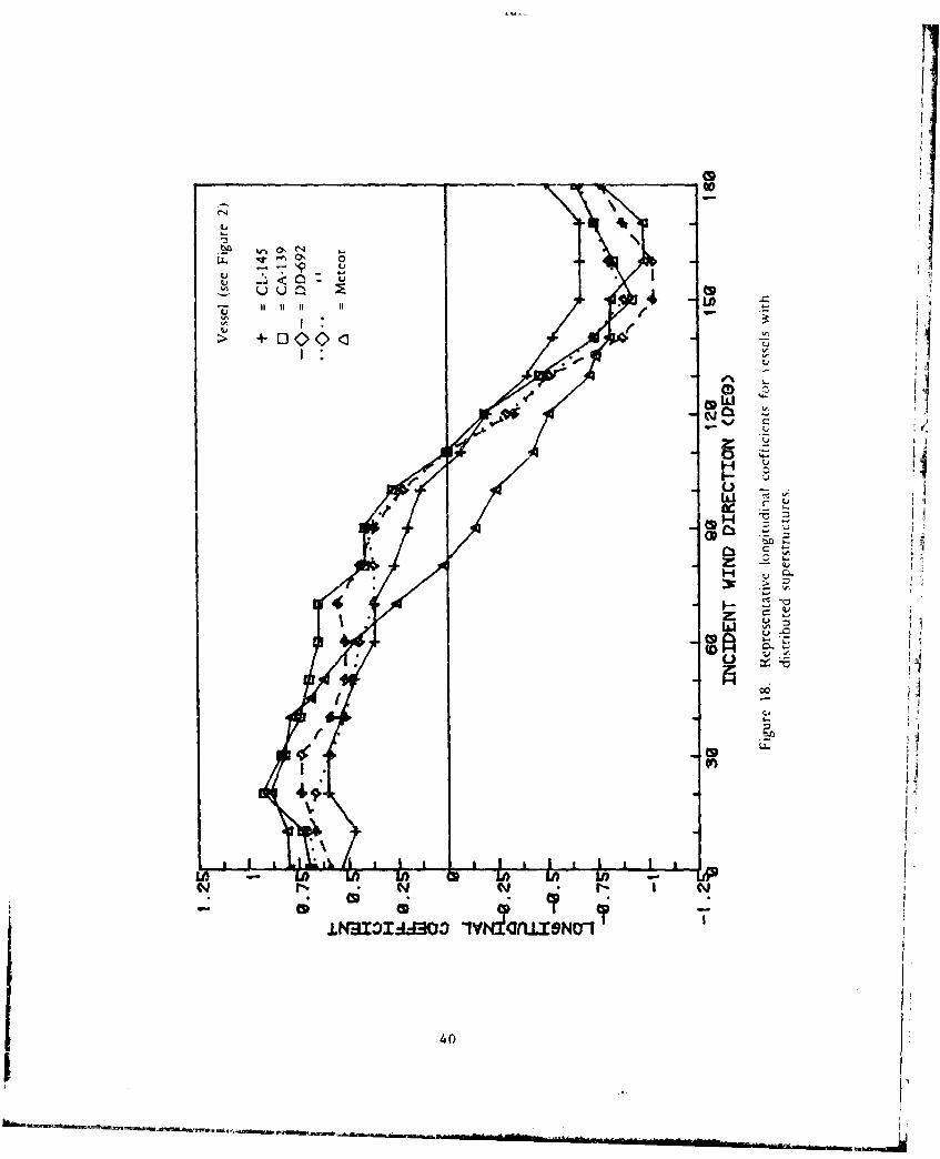
Figures 16 through 19 illustrate longitudinal coefficients (CX) for

most ships and allow for an evaluation of the design procedures recommended

here. Figure 16 shows CX values for the simplest, type of ships; the re-

commendations for C = 0.70, a cosine shape function, and ".ariable zeroXB

-rossing values are reasonable for this application. Figure 17 shows C

XBXvalues for center island tankers; the recommendations of C XB =_ 0.8 or

CXB 0 .9, a humped cosine shape function, and 6 e 100 degrees areXE Z

demonstrated. Similarly, Figure 18 shows C values for ships with

distributed superstructures; note that C values are larger than

CXB values, as noted in the SUNMARY OF WIND FORCE EQUATIONS section.

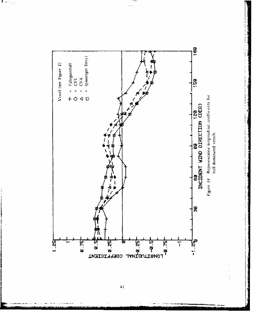
Finally, Figure 19 shows bull dominated vessels; note the extreme

Z ~ 120 degree value, and the extreme behavior of the "Fahrgastshiff"

(see Figure 2 for silhouette). Otherwise, the results are nearly

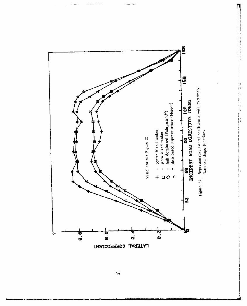
identical.Figures 20 through 22 show representative lateral coefficients

(C ). However, only a discussion on the shape function is applicable

here, since the design methods presented in this report allow for variable

values of the peak coefficient.

Figure 20 shows the "usual" sinusoidal shape function used by most

designers. As shown, this shape function certainly applies to these

vessels. However, Figure 21 shows the type of behavior recommended in

this report as typical for most ships. The flattened behavior of these

responses are evident; in fact, more vessels fez' into this category

than the former. Figure 22 shows an even more extreme type of behavior

measured for some ships, which seems to suggest a "double-humped" behavior.

16

With all three of these figures, no clear indications as to vessel

types versus shape category types were discovered, and the middle-of-the

road shape of Figure 21 was used as generally applicable to all ships.

It is evident now why the general form of the shape function was retained

in Equations 3 and 6; it a2lows the user to easily tailor the charac-

teristic shape of the load versus angle to whatever is considered best.

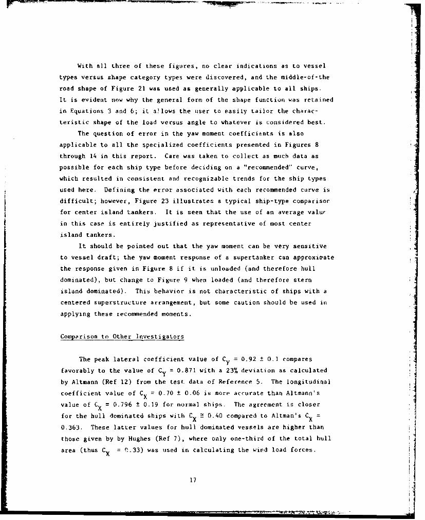
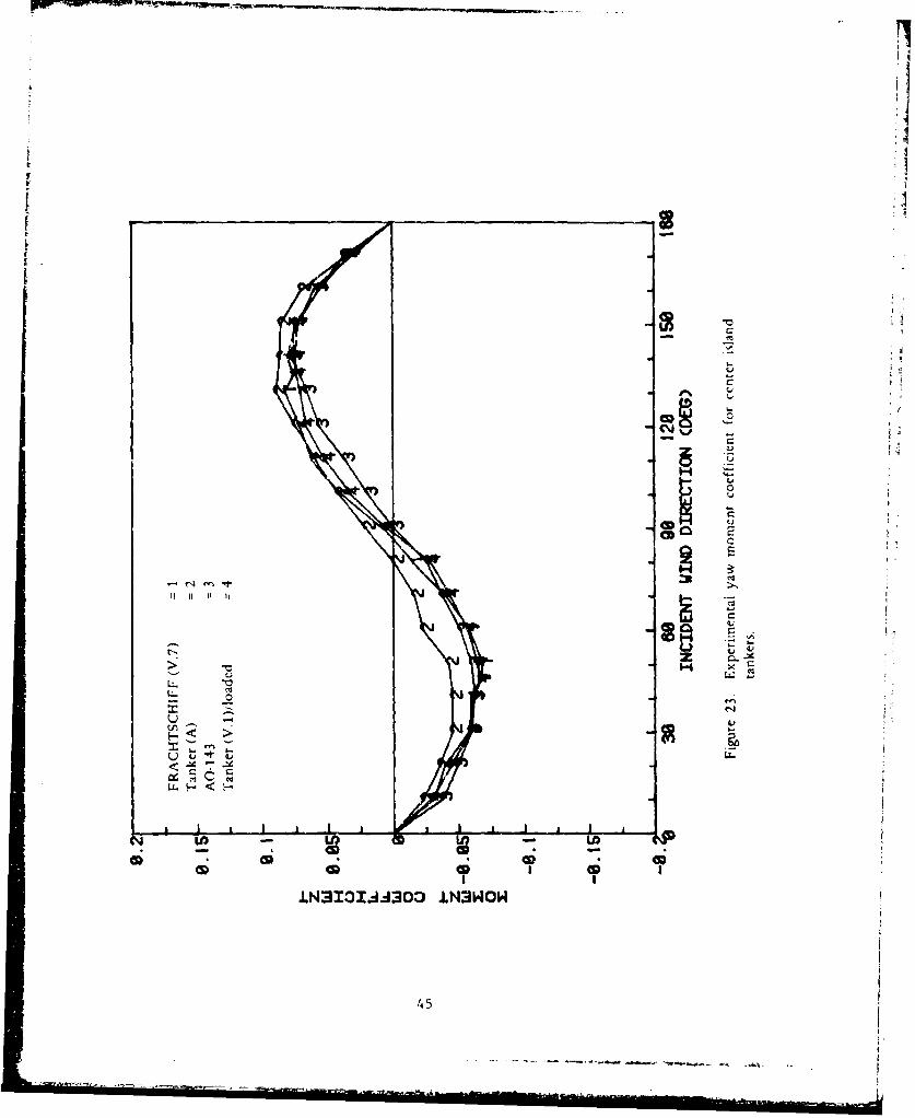
The question of error in the yaw moment coefficients is also

applicable to all the specialized coefficients presented in Figures 8

through 14 in this report. Care was taken to collect as much data as

possible for each ship type before deciding on a "recommended" curve,

which resulted in consistent and recognizable trends for the ship types

used here. Defining the error associated with each recommended curve is

difficult; however, Figure 23 illustrates a typical ship-type comparisor.

for center island tankers. It is seen that the use of an average valur

in this case is entirely justified as representative of most center

island tankers.

It should be pointed out that the yaw moment can be very sensitive

to vessel draft; the yaw moment response of a supertanker can approximate

the response given in Figure 8 if it is unloaded (and therefore hull

dominated), but change to Figure 9 when loaded (and therefore stern

island dominated). This behavior is not characteristic of ships with a

centered superstructure arrangement, but some caution should be used in

applying these recommended moments.

Comparison to Other Investigators

The peak lateral coefficient value of Cy = 0.92 ± 0.1 compares

favorably to the value of Cy = 0.871 with a 23% deviation as calculated

by Altmann (Ref 12) from the test. data of Reference 5. The longitudinal

coefficient value of CX = 0.70 ± 0.06 is more accurate than Altmann's

value of CX = 0.796 ± 0.19 for normal ships. The agreement is closer

for the hull dominated ships with Cx 2 0.40 compared to Altman's CX0.363. These latter values for hull dominated vessels are higher than

those given by by Hughes (Ref 7), where only one-third of the total hull

area (thus CX = q-33) was used in calculating the wind load forces.

17

ji.W

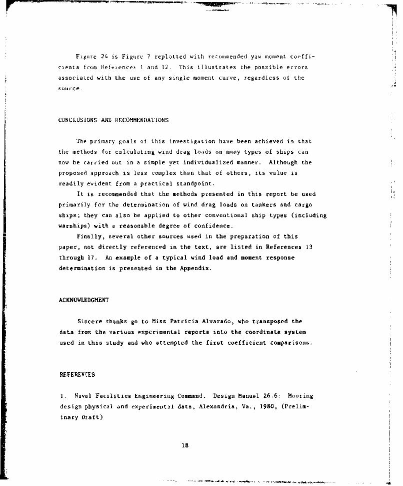
Figure 24 is Figure 7 replotted with recommended yaw moment coeffi-

cients from References I and 12. This illustrates the possible errors

associated with the use of any single moment curve, regardless oi the

source.

CONCLUSIONS AND RECOMMENDATIONS

The primary goals of this investigation have been achieved in that

the methods for calculating wind drag loads on many types of ships can

now be carried out in a simple yet individualized manner. Although the

proposed approach is less complex than that of others, its value is

readily evident from a practical standpoint.

It is recomended that the methods presented in this report be used

primarily for the determination of wind drag loads on tankers and cargo

ships; they can also be applied to other conventional ship types (including

warships) with a reasonable degree of confidence.

Finally, several other sources used in the preparation of this

paper, not directly referenced in the text, are listed in References 13

through 17. An example of a typical wind load and moment response

determination is presented in the Appendix.

ACKNOWLEDGMENT

Sincere thanks go to Miss Patricia Alvarado, who transposed the

data from the various experimental reports into the coordinate system

used in this study and who attempted the first coefficient comparisons.

REFERENCES

1. Naval Facilities Engineering Command. Design Manual 26.6: Mooring

design physical and experimental data, Alexandria, Va., 1980, (Prelim-

inary Draft)

18

2. P. A. Palo and R. L. Webster. "Static and dynamic moored tanker

response," in Computational Methods for Offshore Structures, t-dlted

by H. Armen and S. Stiansen. New York, American SocieLy of Mechanical

Engineers, 1980, pp. 135-146 (AMD, vol 37).

3. V. B. Wagner. "Windkr~fte and Lberwassersciiffen," Schiff Und

Haten, Hamburg, 1967.

4. Naval Facilities Engineering Command. Design Manual DM-26: Harbors

ard coastal facilities, Alexandria, Va., 1968.

5. K. D. A. Shearer and W. M. Lynn. "Wind tunnel tests on models of

merchant ships," International Shipbuilding Progress, vol 8, no. 78,

Feb 1961, pp. 62-80.

6. G. R. tutimer. Wind tunnel tests to determine aerodynamic forces and

moments on ships at zero heel, David Taylor Naval Ship Research and

Development Center, Report 956, Aero Data Report 27, Ma6r 1955.

7. G. Hughes. "Model experiments on the wind resistance of ships,"

Institution of Naval Architects, Transactions, vol 72, 1930, pp. 310-325;

discussion, pp. 326-330.

8. R. W. F. Gould. Measurements of the wind forces on a series of models

of merchant ships, National Physical Laboratory, Aerodynamics Division,

Teddington, U. K., Aero Report 1233, Apr 1967.

9. J. J. Myers, et al, eds. Handbook of ocean and underwater engineering.

New York, McGraw-Hill, 1969.

10. Columbia University, Hudson Laboratories. Report No. ARTEMIS-65-

Vol. 1: A dynamic position keeping system installed aboard the USNS Mission

Capistrano (TAG - 162), vol 1. Preliminary design considerations and

installation, by H. C. Beck and J. 0. Ess. Dobbs Ferry, N.Y., Aug 1968.

(AD 860 376L)

19

S ~,re -~- 5 .. ~ ~.%

F. Hoerner. Fluid-dynamic drag. Midland Park, New Jerscy, 1965.

12. R. Altmann. Forces on ships moored in protected waters, Hydronautics,

Inc., Technical Report 7096-1, 1971, Laurel, MD.

13. G. F. M. Remery and G. von Oortmerssen. "The mean wave, wind and

current forces on offshore structures and their role in the design of

mooring .stems," in Preprints, 5th annual Offshore Technology Conference,

vol 1, pp. 169-184, Dallas, Texas, 1973. (OTC 1741)

14. R. M. Isherwood. "Wind resistance of merchant ships," Royal Institution

of Naval Architects, Supplementary Papers, vol 115, Nov 1973, pp. 327-338.

15. British Ship Research Association. Report NS. 256: Research

investigation for the improvement of ship mooring methods, prepared by

Chamber of Shipping of the United Kingdom. Wallsend, Northcumberland,England, 1969.

16. David W. Taylor Naval Ship Research and Development Center.

Report SPD-716-01: A survey of wind loads on ocean facility structures,

by N. T. Tsai. Bethesda, MD, Aug 1977. (AD A047800)

17. Oil Companies International Marine Forum. Prediction of wind and

current loads on VLCC's, London, 1977.

20

NOMENC LATURE

A,, Lateral projected area of the hull only

AS Lateral projected area of the superstructure only

AX Toongitudinal projected area of the ship

Ay Lateral projected area of the ship

CN Nondimensional yaw moment coefficient

C Nondimensional longitudinal wind force coefficientx

CS Longitudinal headwind (bow) coefficient [Cx at 0 = 0 degrees]

C Longitudinal tailwind (stern) coefficient IC~ at 6 =180 degrees]

C y Nondimensional lateral wind force coefficient

C Calculated peak lateral force coefficient; constant = 0.92 t 0.1

SYM Measured peak lateral force coefficient (from data)

f(O) Normalized shape functions

Fx longitudinal wind force

Fy Y Lateral wind force

N Yaw moment

V Wind velocity

V Reference wind velocity at 33 feet above sea

IR

21

(VH/VR) Average normalized wind velocity over hull

(Vs/VR) Average normalized wind velocity over superstructure

O Incident wind angle with respect to the ship

0 z Zero crossing angle

p Density of air

22 HLI

i ~ ~ f ~ flfj,1 3&.l - --

/,,

-,

U

"0

z PUU -,r

anlv. ±Nx: xaa0

23-

Naval Vcsscls Vessels Used in Figure 6

Uarge Carrier (CVA-59) Cargo A

C.arp, 1. stf

Escoirt Carricr (CVE- iS)

CrrI(frd,

I ica'v Cvu tw (CA- 13Y Ia

ik hcc~chieppci

kI~c!iI, m Rcpn sinI tItv VCSI

Light Cruiki (CL-145)

[)esiruycr MtD-69Z) Ia g tnf

IIrc6rrra.1r

Amphibious Transpron (AI'A-248)

hic y r

me_

I.ibcrty SIlip jdC-2)I anker A

1I-AC, Navy l'anlsci (AO-143) (,argr (

Figure 2. Representative vessel piofiles taken from the total listing in Table 1.

24s

Variable Wind Gradientsleight Above Sea (ft) (N 5, 7, 10)

V9 ( -) =( h96- 7

hR = 33 ft

80

54

48-

32--

16-

0 0.2 0.4 0.6 0.8 1.0 1.2 1.4

Figure 3. Wind gradient family.

25

- -w-~~---

Ii

I

-

[I.'0

amIAJ 0A -~

- C

F'0

Ca'

26

MIS,

W r2to

kC

LL

27J

LIJ bI

0 QN

C1-2: 0 -,

0 '0 -3

;C~q ;I-n :

280

pi:

I.

E:

M d

4 ILI

L.II

S E

S..

IN - w ,,,cc

29

Icl

H

I La.I

(~ri ~ IN3131IJi303 £N3WOW

30

IN31ZAA1 INW311

h3c

S-h EI

F *AU7 in w

IN3=141 I~g-c

32I

ZJ

431IN13JJ0 >'1W

33K

ci a;

I-

IN313JJ= N3WI

34I

, c

CDDIN313JA303IN3WU

353

AoA

0N11J0 jNWO36

I'

II

0*1~~

//

II

- Vo0~EU

/ 0

UC-~

0I 0'U

C I -

4J VQ IU

N

37

- .-- ~ -- ----..-- ~.-~.----- -

CC4))

u I- M

ej uD -I A DL

CO

- U38

L)-. i

I-L

j

INZM1AAM l~~anl9N0

39aJI

> +I

U

00

040 NCH?

IN3131~~~-4.0 tJl8N-T

40-

+-

> Ulu LL. uI

-Cq LL

UC

~4-~ - C

Ccc

CR

41

I S C

CR1

~CID

CI elS

42lut

Lo

ICE CJ'-'*

CP

-~ ~ t H

O- N

soo

j 43

Uaj

C s

I- l

1wU

> I

CD ty

Uy~y

44

Ii

It

i

i

4-)

UU

0UU

4)

10U I-

C0 S

-~ r~.) ~tI! II I' 1.

1.~

Ij~r-. U

0(N

U - _ 4)I-

~Uu

I i I i I ,

(44 ~fl - -

* * * I II I

iN~I3J443O3 .LN~WOW

/45

* E

E >

IN11A0 INWO

* I "~46

6h,

Appendix

SAMPLE PROBLEM

For demonstration purposes, the following example of the wind load

determination for the center island tanker S. S. Pennsylvania (Figure A-l)

is presented for an arbitrary 30 knot wind. Refer to the summary section

for the expressions used in this example.

Figure A-i. S. S. Peanslyvania

47

Projected areas of vessel, as estimated from Figure A-i, and known vessel

dimensions are:

Ay/ = 19,390 ft2

All = 16,660 ft2

A S = 2,730 ft2

AX = 4,500 ft2

L = 595 ft

Wind Gradient Approximations and Cy

Average height of freeboard = 14 ft (0 - 28 ft)

Average height of superstructure = 43 ft (28 - 57)

Normalized local wind speed is taken from the wind gradient curve (Figure 3),

with n = 7:

0 to 28 ft .......... .(VH/VR) 2 0.60

28 to 57 ft .......... (VS/VR)2 = 1.11

Such that

Cyl= (0.92) (1.11)(2,730) t (0.60)(16,660) = 0.62

19,390

Thus, for the lateral force in a 30 knot wind, from Equation 1,

F~8) 1 2F y (0) p Ay V CYMf(e)

S(0.00237 lb-sec 2/ft 4)(19,390 ft 2)(30 kt)2

22

(1.688 ft/sec/kt) 2(O.62)f(0)

4B

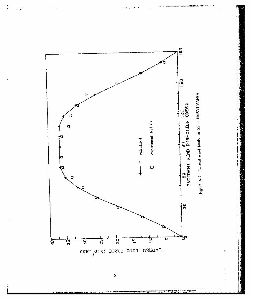
Substituting f(O) from Equation 3, or using Figure 4, lateral force

= (3.66 x l04 sin e - (sin 50)!200.95

This lateral foree is shown in Figure A-2, along with Reynold's Number-

scaled experimental data. Since no information as to the ship's loading

condition (and therefore projected areas) is available from the test

report, the experimental data should be used only as a qualitative check

on the geaeral behavior of the calculated loads. The particulai shape

function recommended by this report is shown to be a good fit to the

experimental data.

CX. The initial mean longitudinal coefficient value is C 0.70X* XB

(t 0.06), but since the SS PENNSYLVANIA is a center island tanker with

uncluttered decks, the coeffiient is adjusted to C XB 0.70 + 0.10 = 0.80

And, for center island tankers,

S ~ 3/4 CXB 0.60; 0 ! 100 degrees

Such that, for 6 < 0 z

1 2 42

= (0.00237 lb-sec 2/ft 4)(4,500 ft2 )(30 kt) 2

22(1.688 ft/sec/kt)2(O.80)f(O +

Sutstituting for f6Jo) from Equations 6 and 7,

Fx(0 = 1.09x~4) (sin , (sin 5 F)/O) (lb)

&nd

4 = (0.9) 0 + 90

The lcngitudinal force for > 0 is identical to the above equation,z

except C XS 0.60 is used, and Equation 8 is used for ts:

,F = g + 67.5

49

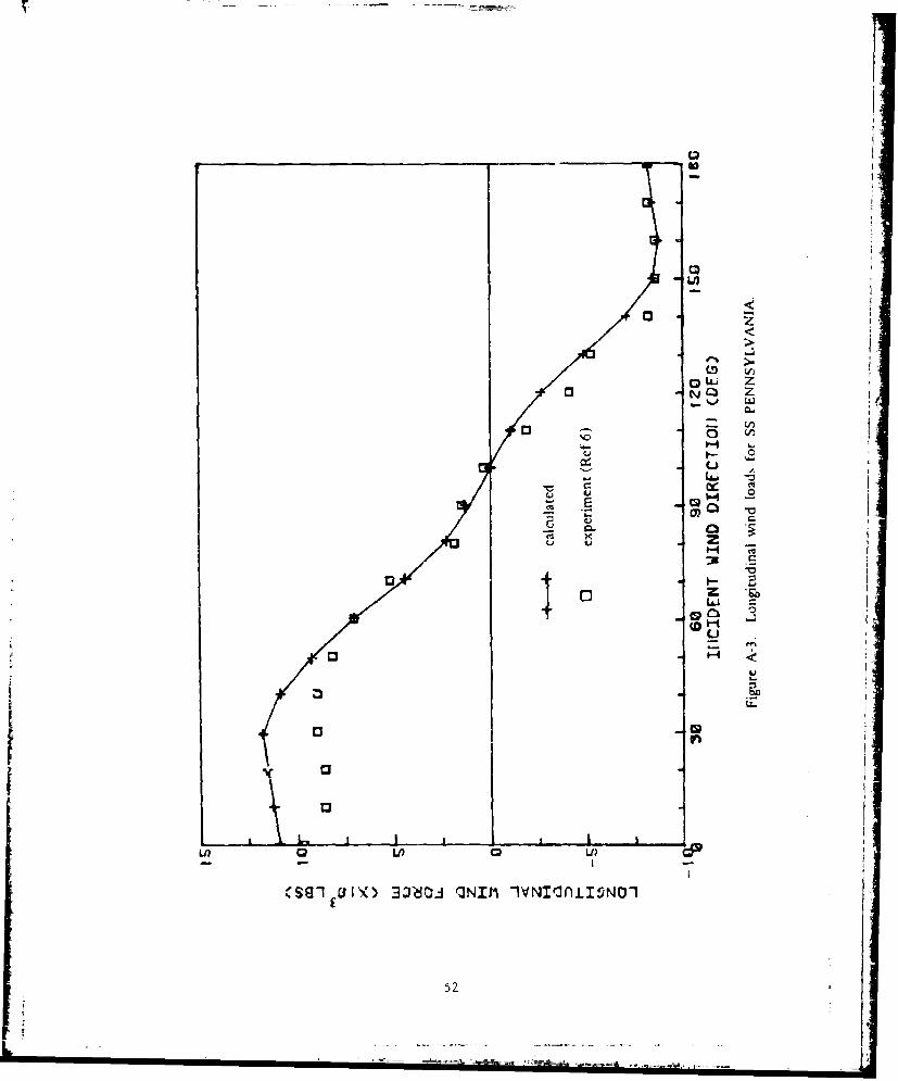
The longitudinal force for this tanker is illustrated in Figure A-3,

along with Reynold's Number-scaled experimental data. Again, because

the projected area of the model in unknown, only a qualitative check is

possible. This shape function, with its "skewed" benavior around 1000

and the flattened tails, shows the same characteristic behavior as the

experi tal results.

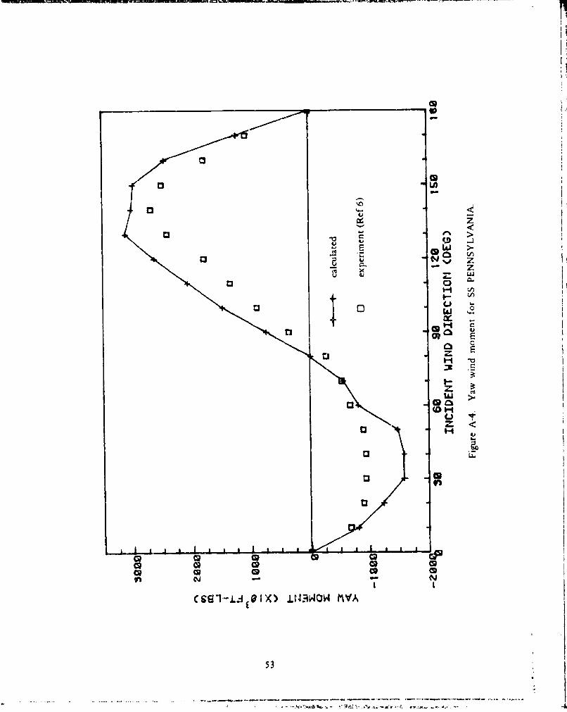
N. The recommended wind i iucJ yaw moment coefficient, CN(),

for a trim center island tanker is shown in Figure 13. The moment

is calculated using Equation 1:

1 V2N V Ay LcN C(e)

- (0.0237 lb-sec 2/ft 4)(30 kt) 2(1.688 ft/sec/kt)

(19,380 ft 2)(595 ft) CN (0)

7= (3.5 x 107) CN (8) (ft-lb)

The moment is shown in Figure A-4, along with Reynold's Number-scaled

experimental data.

The ship used in this example could be claszified as a "center-balanced

superstructure" ship, so the yaw moment coefficients recommended in

Peference I and shown as dotted in Figure 16 could have been used instead

of the specialized curves in Figure 13. A comparison of N (0) values

between Figures 13 and 16 shows that this alternate function would have

overestimated the measured minimmn and maximum yaw moments by approxi-

mately 100%. This clearly demonstrates the potential errors of using

a too simplistic loading function in the moment estimation.

50

UIi

Q

Lu

VI'

C;I

H

LZ

......... .. ........LA th L) Ln Lip L

0% ONKj Cc Gl 0N) AJO3 1NIM-lV31V

511 .

7p 4

0 -j

zl

40 v7-Z

I- i

3J80 IN.- IVV I9

52)

00

0U

M

cl0 0

013E13~ 4"S

13O

CD (2

c9 Ij0 1 X) IN OWMV

53

DISTRIBUTION LIST

AFB CESCH, Wright-PattersonARCTICSUBLAB Code 54. San Diego. CAARMY BMDSC-RE (H. McClellan) Huntsville ALARMY COASTAL ENGR RSCH CEN Fort Bclvoir VA: R. Jachowski. Fort Belvoir VAARMY COE Philadelphia Dist. (LIBRARY) Philadelphia. PAARMY CORPS OF ENGINEERS MRD-Eng. Div.. Omaha NE: Seattle Dist. Library. Seattle WAARMY CRREL A. Kovacs. Hanover NH: Library. Hanover NI-ARMY DARCOM Code DRCMM-CS Alexandria VAARMY ENG WATERWAYS EXP STA Library. Vicksburg MSARMY ENGR DIST. Library. Portland ORARMY ENVIRON. HYGIENE AGCY HSE-EW Water Oual Eng Div Aberdeen Prov Grnd MDARMY MATERIALS & MECHANICS RESEARCH CENTER Dr. Lcnoe. Watertown MAARMY TRANSPORTATION SCHOOL Code ATSPO CD-TE Fort Eustis. VAASST SECRETARY OF THE NAVY Spec. Assist Submarines, Washington DCBUREAU OF RECLAMATION Code 1512 (C. Selander) Denver COCNM MAT-0718. Washington. DC: NMAT- 044. Washington DCCNO Code NOP-964, Washington DC: Code OP 323. Washington DC: Code OPNAV 091B24 (H): Code OPNAV

22. Wash DC; Code OPNAV 23. Wash DC: OP-23 (Capt J.H. Howland) Washinton. DC: OP987J (J.Boosman), Pentagon

COMNAVBEACHPHIBREFTRAGRU ONE San Diego CACOMSUBDEVGRUONE Operations Offr. San Diego. CADEFENSE INTELLIGENCE AGENCY DB-4CI Washington DCDEFFUELSUPPCEN DFSC-OWE (Grafton) Alexandria. VADTIC Defense Technical Info Ctr/Alexandria. VAHCU ONE CO. Bishops Point. HILIBRARY OF CONGRESS Washington. DC (Scicnrc'. & Tech Div)MCAS Facil. Engr. Div. Cherry Point NCMILITARY SEALIFT COMMAND Washington DCNAF PWO. Atsugi JapanNALF OINC. San Diego. CANARF Equipment Engineering Division (Code 61(000). Pensacola. FLNAS Dir. Util. Div., Bermuda: PWD - Engr Div. Oak Harbor. WA: PWD Maint. Div.. New Orleans. Belle

Chasse LA; PWD. Code 1821H (Pfankuch) Miramar. SD CA: PWO Belle Chasse. LA: PWO Key West FL:PWO. Glenview IL: SCE Norfolk. VA: Shore Facil. Ofr Norfolk. VA

NATL BUREAU OF STANDARDS Kovacs. Washington. D.C.NATL RESEARCH COUNCIL Naval Studies Board. Washington DCNAVACT PWO. London UKNAVAEROSPREGMEDCEN SCE. Pensacola FLNAVAIRDEVCEN Code 813. Warminster PANAVCOASTSYSTCTR CO. Panama City FL: Code 715 (1 Quirk) Panama City. FL: Code 715 (J. Mittleman)

Panama City, FL: Library Panama City. FL: PWO Panama City. FLNAVCOMMAREAMSTRSTA SCE Unit I Naples ItalyNAVCOMMSTA Code 401 Nea Makri. Greece: PWD - Maint Control Div. Diego Garcia Is.: PWO. Exmouth.

AustraliaNAVEDTRAPRODEVCEN Technical Library. Pensacola, FLNAVELEXSYSCOM Code PME 124-61. Washington. DC: PME 124-612. Wash DCNAVEODFAC Code 605, Indian Head MDNAVFAC PWO. Centerville Bch. Ferndale CANAVFACENGCOM Code 03T (Essoglou) Alexandria, VA: Code 043 Alexandria. VA: Code 044 Alexandria.

VA: Code 0453 (D. Potter) Alexandria. VA: Code 0453C. Alexandria. VA: Code 04AI Alexandria. VA:Code 100 Alexandria. VA: Code l(X)2B (J. Leimanis) Alexandria. VA:.Code 1113 (T. Stevens) Alexandria.VA; Morrison Yap. Caroline Is.: ROICC Code 495 Portsmouth VA

NAVFACENGCOM - CHES DIV. Code 407 (D Scheesele) Washington. DC: Code FPO-IC Washington DC:FPO-I Washington. DC: FPO-IEA5 Washington DC

NAVFACENGCOM - LANT DIV. Eur. BR Deputy Dir. Naples Italy: RDT&ELO 102. Norfolk VANAVFACENGCOM - NORTH DIV. (Boretsky) Philadelphia. PA: CO: Code 04 Philadelphia, PA: Code 1028.

RDT&ELO. Philadelphia PA: ROICC. Contracts. Crane INNAVFACENGCOM - PAC DIV. CODE 09P PEARL HARBOR HI: Code 402. RDT&E. Pearl Harbor HI:

Commander. Pearl Harbor. HINAVFACENGCOM - SOUTH DIV. Code 90. RDT&ELO. Charleston SCNAVFACENGCOM WEST DIV. Code 04B San Bruno. CA. 09P/20 San Bruno. CA: RDT&ELO Code 2011

San Bruno. CA

54

NAVFACENGCOM CONTRACT Eng Div dir. Southwest Pac. Manila. P1; OICC. Southwest Pac. Manila, PI.

OICC/ROICC, Balboa Panama Canal: ROICC. NAS. Corpus Christi. TXNAVOCEANO Library Bay St. Louis. MSNAVOCEANSYSCEN Code 41. San Diego. CA: Code 4473 Bayside Library. San Diego. CA: Code 4473B

(Tech Lib) San Diego. CA: Code 52 (H. Talkington) San Diego CA" Code 5204 J. Stachiw). San Diego,

('A. Code 5214 (11. Wheeler). San Diego CA: Code 5221 (R.Jones) San Diego Ca: Code 5311 (Bachman)

San Diego. CA: Hawaii Lab (R Yumori) Kaihia. HI; Hi Lab Tech Lib Kailua HI

NAVPGSCOL C. Morers Monterey CA: E. Thornton. Monterey CA

NAVPHIBASE CO. ACB 2 Norfolk. VA: COMNAVBEACHGRU TWO Norfolk VA: Code S3T. Norfolk VA:

Harbor Clearance Unit Two. Little Creek. VA; SCE. Coronado. San Diego CANAVREGMEDCEN SCE (D. Kaye)

NAVSEASYSCOM Code PMS 395 A 3. Washington. DC: Code SEA OOC Washington. DC

NAVSHIPREPFAC Library. Guam: SCE Subic Bay

NAVSHIPYD Bremerton. WA (Carr Inlet Acoustic Range): Code 202.4. Long Beach CA: Code 440

Portsmouth NH: Code 440. Puget Sound. Bremerton WA: Tech Library. Vallejo. CA

NAVSTA CO Roosevelt Roads P.R. Puerto Rico: Dir Engr Div. PWD. Mayport FL: PWD (LTJG.P.M.Motolenich). Puerto Rico: PWO Pearl Harbor. HI: PWO. Keflavik Iceland: PWO. Mayport FL- SCE. Guam:

SCE, Subic Bay. R.P.: Security Offr. San Francisco. CANAVTECHTRACEN SCE. Pensacola FLNAVWPNCEN Code 3803 China Lake. CANAVWPNSTA Code 092. Colts Neck NJNAVWPNSTA PW Office Yorktown. VANAVWPNSTA PWD - Maint. Control Div.. Concord. CA: PWD - Supr Gen Engr. Seal Beach. CA- PWO.

Charleston. SC; PWO. Seal Beach CANAVWPNSUPPCEN Code 09 Crane INNCBC Code 10 Davisville. RI: Code 15. Port Hueneme CA: Code 155. Port Hueneme CA: Code 156. Port

Hueneme. CANMCB FIVE. Operations DeptNOAA (Dr. T. Mc Guinness) Roek%7ile. MD: Library Rockville. MD

NORDA Code 410 Bay St. Louis. MS: Code. 440 (Ocean Rsch Off Bay St. Louis MS

NRL Code 58() Washington. DC: Code 5843 (F. Rosenthal) Washington. DC: Code 8441 (R.A. Skop).

Washington DCNROTC J.W. Stephenson. UC. Berkeley. CANSI) SCE. Subic Bay. R.P.

NUCLEAR REGULATORY COMMISSION T.C. Johnson. Washington. DC

NUSC Code 131 New London. CT: Code 332. B-80I (J. Wilcox) New London. CT: Code EA123- (R.S. Munn),

New London CT: Code TAi31 (G. De la Cruz). New London CT

ONR (Scientific Dir) Pasadena. CA: Central Regional Office. Boston. MA: Code 481, Bay St. Louis. MS:

Code 485 (Silva) Arlington. VA: Code 7(X)F Arlington VA

PHIBCB I P&E. San Diego, CA; I. CO San Diego. CA

PMTC Code 3331 (S. Opatowsky) Point Mugu. CA: EOD Mobile Unit. Point Mugu. CA: Pat. Counsel. Point

Mugu CAPWC CO Norfolk. VA: CO. (Code 10). Oakland. CA: CO. Great Lakes IL: CO. Pearl Harbor III: Code 10.

Great Lakes, IL: Code 12(0. Oakland CA: Code 120C. (Library) San Diego. CA: Code 128. Guam: CodeI154. Great Lakes. IL: Code 20. Great Lakes IL: Code 30C. Norfolk. VA: Code 30C. San Diego. CA. Code

400. Great Lakes. IL; Code 4MX). Pearl Harbor, HI: Code 4(M). San Diego. CA; Code 420. Great Lakes, IL:

Code 420. Oakland, CA: Code 7X), San Diego. CA

UCTr ONE OIC, Norfolk. VA: UCT TWO OIC, Port Hueneme CA

US DEPT OF INTERIOR Bur of Land Mngmnt Code 583 (T F Sullivan) Washington. DC

US GEOLOGICAL SURVEY Off. Marine Geology. Piteleki. Reston VA

US NAVAL FORCES Korea (ENJ-P&O)USCG (Smith). Washington, DC. G-EOE-4 (T Dowd). Washington. DC

USCG R&D CENTER CO Groton. CT: D. Motherway. Groton CT

USDA Forest Service. San Dimas, CA

USNA Civil Engr Dept (R. Erchyl) Annapolis MD; Ocean Sys. Eng Dept (Dr. Monney) Annapolis. MD: PWD

Engr. Div. (C. Bradford) Annapolis MD

55