4 conventional terrestrial reference system and frame

No.32IERS

TechnicalNote

4 Conventional Terrestrial Reference System and Frame

4.1 Concepts and Terminology

4.1.1 Basic Concepts

A Terrestrial Reference System (TRS) is a spatial reference system co-rotating with the Earth in its diurnal motion in space. In such a system,positions of points attached to the solid surface of the Earth have coordi-nates which undergo only small variations with time, due to geophysicaleffects (tectonic or tidal deformations). A Terrestrial Reference Frame(TRF) is a set of physical points with precisely determined coordinatesin a specific coordinate system (Cartesian, geographic, mapping...) at-tached to a Terrestrial Reference System. Such a TRF is said to be arealization of the TRS. These concepts have been defined extensivelyby the astronomical and geodetic communities (Kovalevsky et al., 1989,Boucher, 2001).Ideal Terrestrial Reference Systems. An ideal Terrestrial ReferenceSystem (TRS) is defined as a reference trihedron close to the Earth andco-rotating with it. In the Newtonian framework, the physical space isconsidered as an Euclidian affine space of dimension 3. In this case, sucha reference trihedron is an Euclidian affine frame (O,E). O is a point ofthe space named origin. E is a basis of the associated vector space. Thecurrently adopted restrictions on E are to be right-handed, orthogonalwith the same length for the basis vectors. The triplet of unit vectorscollinear to the basis vectors will express the orientation of the TRSand the common length of these vectors its scale,

λ = ‖ ~Ei‖i=1,2,3. (1)

We consider here systems for which the origin is close to the Earth’scenter of mass (geocenter), the orientation is equatorial (the Z axis is thedirection of the pole) and the scale is close to an SI meter. In additionto Cartesian coordinates (naturally associated with such a TRS), othercoordinate systems, e.g. geographical coordinates, could be used. For ageneral reference on coordinate systems, see Boucher (2001).Under these hypotheses, the general transformation of the Cartesiancoordinates of any point close to the Earth from TRS (1) to TRS (2) willbe given by a three-dimensional similarity (~T1,2 is a translation vector,λ1,2 a scale factor and R1,2 a rotation matrix)

~X(2) = ~T1,2 + λ1,2 ·R1,2 · ~X(1). (2)

This concept can be generalized in the frame of a relativistic backgroundmodel such as Einstein’s General Relativity, using the spatial part ofa local Cartesian frame (Boucher, 1986). For more details concerninggeneral relativistic models, see Chapters 10 and 11.In the application of (2), the IERS uses the linearized formulas and no-tation. The standard transformation between two reference systems is aEuclidian similarity of seven parameters: three translation components,one scale factor, and three rotation angles, designated respectively, T1,T2, T3, D, R1, R2, R3, and their first time derivatives: T1, T2, T3, D,R1, R2, R3. The transformation of a coordinate vector ~X1, expressed inreference system (1), into a coordinate vector ~X2, expressed in referencesystem (2), is given by

~X2 = ~X1 + ~T +D ~X1 +R ~X1, (3)

λ1,2 = 1 +D, R1,2 = (I +R), and I is the identity matrix with

21

No.32 IERS

TechnicalNote


T =

(T1T2T3

), R =

( 0 −R3 R2R3 0 −R1−R2 R1 0

).

It is assumed that equation (3) is linear for sets of station coordinatesprovided by space geodesy techniques. Origin differences are about a fewhundred meters, and differences in scale and orientation are at the levelof 10−5. Generally, ~X1, ~X2, T , D,R are functions of time. Differentiatingequation (3) with respect to time gives

~X2 = ~X1 + ~T + D ~X1 +D ~X1 + R ~X1 +R ~X1. (4)

D and R are at the 10−5 level and X is about 10 cm per year, theterms D ~X1 and R ~X1 which represent about 0.1 mm over 100 years arenegligible. Therefore, equation (4) could be written as

~X2 = ~X1 + ~T + D ~X1 + R ~X1. (5)

Conventional Terrestrial Reference System (CTRS). A CTRS isdefined by the set of all conventions, algorithms and constants whichprovide the origin, scale and orientation of that system and their timeevolution.Conventional Terrestrial Reference Frame (CTRF). A Conven-tional Terrestrial Reference Frame is defined as a set of physical pointswith precisely determined coordinates in a specific coordinate systemas a realization of an ideal Terrestrial Reference System. Two types offrames are currently distinguished, namely dynamical and kinematical,depending on whether or not a dynamical model is applied in the processof determining these coordinates.

4.1.2 TRF in Space Geodesy

Seven parameters are needed to fix a TRF at a given epoch, to whichare added their time-derivatives to define the TRF time evolution. Theselection of the 14 parameters, called “datum definition,” establishes theTRF origin, scale, orientation and their time evolution.Space geodesy techniques are not sensitive to all the parameters of theTRF datum definition. The origin is theoretically accessible through dy-namical techniques (LLR, SLR, GPS, DORIS), being the center of mass(point around which the satellite orbits). The scale depends on somephysical parameters (e.g. geo-gravitational constant GM and speed oflight c) and relativistic modelling. The orientation, unobservable by anytechnique, is arbitrary or conventionally defined. Meanwhile it is recom-mended to define the orientation time evolution using a no-net-rotationcondition with respect to horizontal motions over the Earth’s surface.Since space geodesy observations do not contain all the necessary in-formation to completely establish a TRF, some additional informationis then needed to complete the datum definition. In terms of normalequations, usually constructed upon space geodesy observations, thissituation is reflected by the fact that the normal matrix, N , is singular,since it has a rank deficiency corresponding to the number of datumparameters which are not reduced by the observations.In order to cope with this rank deficiency, the analysis centers currentlyadd one of the following constraints upon all or a sub-set of stations:

1. Removable constraints: solutions for which the estimated stationpositions and/or velocities are constrained to external values within

22

4.1 Concepts and Terminology

No.32IERS

TechnicalNote

an uncertainty σ ≈ 10−5 m for positions and m/y for velocities.This type of constraint is easily removable, see for instance Al-tamimi et al. (2002a; 2002b).

2. Loose constraints: solutions where the uncertainty applied to theconstraints is σ ≥ 1 m for positions and ≥ 10 cm/y for velocities.

3. Minimum constraints used solely to define the TRF using a min-imum amount of required information. For more details on theconcepts and practical use of minimum constraints, see for instanceSillard and Boucher (2001) and Altamimi et al. (2002a).

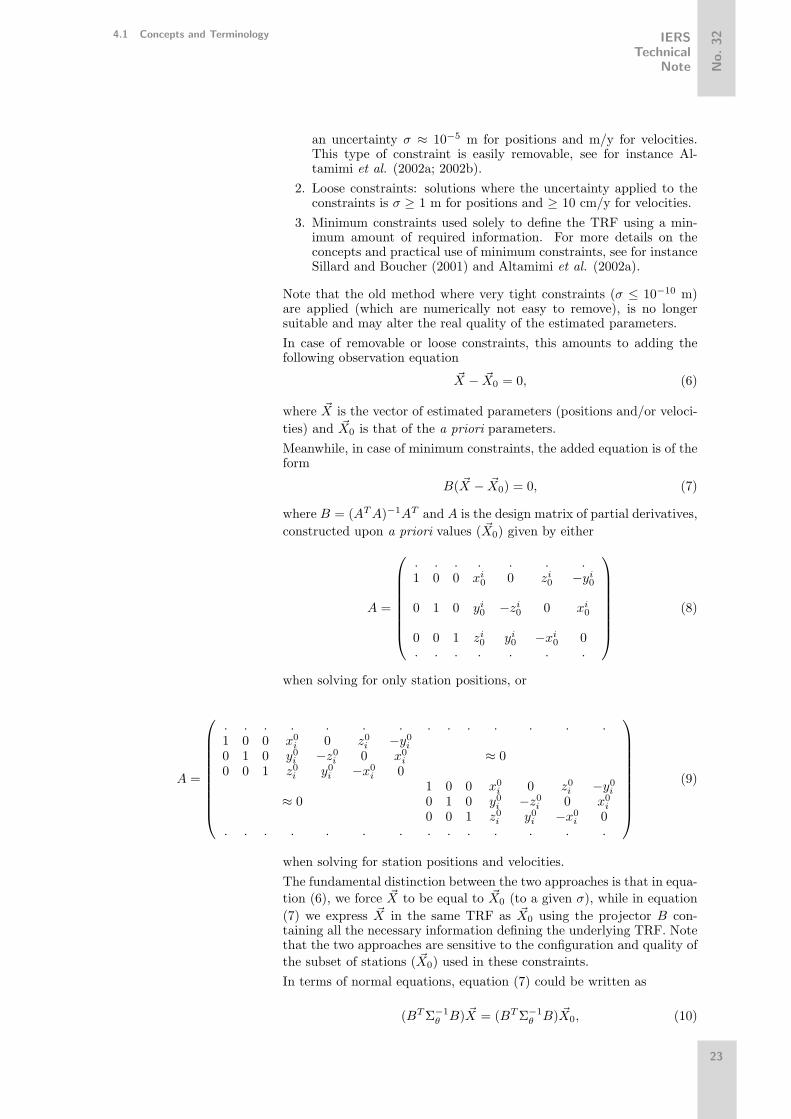
Note that the old method where very tight constraints (σ ≤ 10−10 m)are applied (which are numerically not easy to remove), is no longersuitable and may alter the real quality of the estimated parameters.In case of removable or loose constraints, this amounts to adding thefollowing observation equation

~X − ~X0 = 0, (6)

where ~X is the vector of estimated parameters (positions and/or veloci-ties) and ~X0 is that of the a priori parameters.Meanwhile, in case of minimum constraints, the added equation is of theform

B( ~X − ~X0) = 0, (7)

where B = (ATA)−1AT and A is the design matrix of partial derivatives,constructed upon a priori values ( ~X0) given by either

A =

. . . . . . .1 0 0 xi

0 0 zi0 −yi

0

0 1 0 yi0 −zi

0 0 xi0

0 0 1 zi0 yi

0 −xi0 0

. . . . . . .

(8)

when solving for only station positions, or

A =

. . . . . . . . . . . . . .1 0 0 x0

i 0 z0i −y0

i

0 1 0 y0i −z0

i 0 x0i ≈ 0

0 0 1 z0i y0

i −x0i 0

1 0 0 x0i 0 z0

i −y0i

≈ 0 0 1 0 y0i −z0

i 0 x0i

0 0 1 z0i y0

i −x0i 0

. . . . . . . . . . . . . .

(9)

when solving for station positions and velocities.The fundamental distinction between the two approaches is that in equa-tion (6), we force ~X to be equal to ~X0 (to a given σ), while in equation(7) we express ~X in the same TRF as ~X0 using the projector B con-taining all the necessary information defining the underlying TRF. Notethat the two approaches are sensitive to the configuration and quality ofthe subset of stations ( ~X0) used in these constraints.In terms of normal equations, equation (7) could be written as

(BT Σ−1θ B) ~X = (BT Σ−1

θ B) ~X0, (10)

23

No.32 IERS

TechnicalNote


where Σθ is a diagonal matrix containing small variances for each ofthe transformation parameters. Adding equation (10) to the singularnormal matrix N allows it to be inverted and simultaneously to expressthe estimated solution in the same TRF as the a priori solution ~X0. Notethat the 7 columns of the design matrix A correspond to the 7 datumparameters (3 translations, 1 scale factor and 3 rotations). Thereforethis matrix should be reduced to those parameters which need to bedefined (e.g. 3 rotations in almost all techniques and 3 translations incase of VLBI). For more practical details, see, for instance, Altamimi etal. (2002a).

4.1.3 Crust-based TRF

In general, various types of TRF can be considered. In practice twomajor categories are used:

• positions of satellites orbiting around the Earth, expressed in a TRS.This is the case for navigation satellite systems or satellite radar al-timetry, see section 4.3;

• positions of points fixed on solid Earth crust, mainly tracking instru-ments or geodetic markers (see sub-section 4.2.1).

Such crust-based TRF are those currently determined in IERS activities,either by analysis centers or by combination centers, and ultimately asIERS products (see sub-section 4.1.5).

The general model connecting the instantaneous actual position of apoint anchored on the Earth’s crust at epoch t, ~X(t), and a regularizedposition ~XR(t) is

~X(t) = ~XR(t) +∑

i

∆ ~Xi(t). (11)

The purpose of the introduction of a regularized position is to removehigh-frequency time variations (mainly geophysical ones) using conven-tional corrections ∆ ~Xi(t), in order to obtain a position with regular timevariation. In this case, ~XR can be estimated by using models and numer-ical values. The current model is linear (position at a reference epoch t0and velocity):

~XR(t) = ~X0 + ~X · (t− t0). (12)

The numerical values are ( ~X0, ~X). In the past (ITRF88 and ITRF89),constant values were used as models ( ~X0), the linear motion being incor-porated as conventional corrections derived from a tectonic plate motionmodel (see sub-section 4.2.2).

Conventional models are presented in Chapter 7 for solid Earth tides,ocean loading, pole tide, atmospheric loading, and geocenter motion.

4.1.4 The International Terrestrial Reference System

The IERS is in charge of defining, realizing and promoting the Inter-national Terrestrial Reference System (ITRS) as defined by the IUGGResolution No. 2 adopted in Vienna, 1991 (Geodesist’s Handbook, 1992).The resolution recommends the following definitions of the TRS: “1)CTRS to be defined from a geocentric non-rotating system by a spa-tial rotation leading to a quasi-Cartesian system, 2) the geocentric non-rotating system to be identical to the Geocentric Reference System(GRS) as defined in the IAU resolutions, 3) the coordinate-time of the

24

4.2 ITRF Products

No.32IERS

TechnicalNote

CTRS as well as the GRS to be the Geocentric Coordinate Time (TCG),4) the origin of the system to be the geocenter of the Earth’s masses in-cluding oceans and atmosphere, and 5) the system to have no globalresidual rotation with respect to horizontal motions at the Earth’s sur-face.”The ITRS definition fulfills the following conditions.

1. It is geocentric, the center of mass being defined for the wholeEarth, including oceans and atmosphere;

2. The unit of length is the meter (SI). This scale is consistent withthe TCG time coordinate for a geocentric local frame, in agree-ment with IAU and IUGG (1991) resolutions. This is obtained byappropriate relativistic modelling;

3. Its orientation was initially given by the Bureau International del’Heure (BIH) orientation at 1984.0;

4. The time evolution of the orientation is ensured by using a no-net-rotation condition with regards to horizontal tectonic motions overthe whole Earth.

4.1.5 Realizations of the ITRS

Realizations of the ITRS are produced by the IERS ITRS Product Cen-ter (ITRS-PC) under the name International Terrestrial Reference Frame(ITRF). The current procedure is to combine individual TRF solutionscomputed by IERS analysis centers using observations of space geodesytechniques: VLBI, LLR, SLR, GPS and DORIS. These individual TRFsolutions currently contain station positions and velocities together withfull variance matrices provided in the SINEX format. The combinationmodel used to generate ITRF solutions is essentially based on the trans-formation formulas of equations (3) and (5). The combination methodmakes use of local ties in collocation sites where two or more geodeticsystems are operated. The local ties are used as additional observationswith proper variances. They are usually derived from local surveys us-ing either classical geodesy or the Global Positioning System (GPS). Asthey represent a key element of the ITRF combination, they should bebetter or at least as accurate as the individual space geodesy solutionsincorporated in the ITRF combination.Currently, ITRF solutions are published nearly annually by the ITRS-PC in the Technical Notes (cf. Boucher et al., 1999). The numbers (yy)following the designation “ITRF” specify the last year whose data wereused in the formation of the frame. Hence ITRF97 designates the frameof station positions and velocities constructed in 1999 using all of theIERS data available until 1998.The reader may also refer to the report of the ITRF Working Group onthe ITRF Datum (Ray et al., 1999), which contains useful informationrelated to the history of the ITRF datum definition. It also detailstechnique-specific effects on some parameters of the datum definition, inparticular the origin and the scale.

4.2 ITRF Products

4.2.1 The IERS Network

The initial definition of the IERS networkThe IERS network was initially defined through all tracking instrumentsused by the various individual analysis centers contributing to the IERS.All SLR, LLR and VLBI systems were included. Eventually, GPS sta-tions from the IGS were added as well as the DORIS tracking network.The network also included, from its beginning, a selection of ground

25

No.32 IERS

TechnicalNote


markers, specifically those used for mobile equipment and those cur-rently included in local surveys performed to monitor local eccentricitiesbetween instruments for collocation sites or for site stability checks.Each point is currently identified by the attribution of a DOMES num-ber. The explanations of the DOMES numbering system is given below.Close points are clustered into a site. The current rule is that all pointswhich could be linked by a collocation survey (up to 30 km) should beincluded as a unique site of the IERS network having a unique DOMESsite number.

CollocationsIn the frame of the IERS, the concept of collocation can be defined as thefact that two instruments are occupying simultaneously or subsequentlyvery close locations that are very precisely surveyed in three dimensions.These include situations such as simultaneous or non-simultaneous mea-surements and instruments of the same or different techniques.As typical illustrations of the potential use of such data, we can mention:

1. calibration of mobile systems, for instance SLR or GPS antennas,using simultaneous measurements of instruments of the same tech-nique;

2. repeated measurements on a marker with mobile systems (for in-stance mobile SLR or VLBI), using non-simultaneous measure-ments of instruments of the same technique;

3. changes in antenna location for GPS or DORIS;4. collocations between instruments of different techniques, which im-

plies eccentricities, except in the case of successive occupancies ofa given marker by various mobile systems.

Usually, collocated points should belong to a unique IERS site.

Extensions of the IERS networkRecently, following the requirements of various user communities, theinitial IERS network was expanded to include new types of systemswhich are of potential interest. Consequently, the current types of pointsallowed in the IERS and for which a DOMES number can be assignedare (IERS uses a one character code for each type):

• satellite laser ranging (SLR) (L),• lunar laser ranging (LLR) (M),• VLBI (R),• GPS (P),• DORIS (D) also Doppler NNSS in the past,• optical astrometry (A) –formerly used by the BIH–,• PRARE (X),• tide gauge (T),• meteorological sensor (W).

For instance, the cataloging of tide gauges collocated with IERS instru-ments, in particular GPS or DORIS, is of interest for the Global SeaLevel Observing System (GLOSS) program under the auspices of UN-ESCO.Another application is to collect accurate meteorological surface mea-surements, in particular atmospheric pressure, in order to derive rawtropospheric parameters from tropospheric propagation delays that canbe estimated during the processing of radio measurements, e.g. made

26

4.2 ITRF Products

No.32IERS

TechnicalNote

by the GPS, VLBI, or DORIS space techniques. Other systems couldalso be considered if it was considered as useful (for instance systemsfor time transfer, super-conducting or absolute gravimeters. . .) Thesedevelopments were undertaken to support the conclusions of the CSTGWorking Group on Fundamental Reference and Calibration Network.

Another important extension is the wish of some continental or nationalorganizations to see their fiducial networks included into the IERS net-work, either to be computed by IERS (for instance the European Ref-erence Frame (EUREF) permanent GPS network) or at least to getDOMES numbers (for instance the Continuously Operating ReferenceStations (CORS) network in USA). Such extensions are supported by theIAG Commission X on Global and Regional Geodetic Networks (GRGN)in order to promulgate the use of the ITRS.

4.2.2 History of ITRF Products

The history of the ITRF goes back to 1984, when for the first time acombined TRF (called BTS84), was established using station coordinatesderived from VLBI, LLR, SLR and Doppler/ TRANSIT (the predecessorof GPS) observations (Boucher and Altamimi, 1985). BTS84 was real-ized in the framework of the activities of BIH, being a coordinating centerfor the international MERIT project (Monitoring of Earth Rotation andInter-comparison of Techniques) (Wilkins, 2000). Three other successiveBTS realizations were then achieved, ending with BTS87, when in 1988,the IERS was created by the IUGG and the International AstronomicalUnion (IAU).

Until the time of writing, 10 versions of the ITRF were published, start-ing with ITRF88 and ending with ITRF2000, each of which supersededits predecessor.

From ITRF88 till ITRF93, the ITRF Datum Definition is summarizedas follows:

• Origin and Scale: defined by an average of selected SLR solutions;

• Orientation: defined by successive alignment since BTS87 whose ori-entation was aligned to the BIH EOP series. Note that the ITRF93orientation and its rate were again realigned to the IERS EOP series;

• Orientation Time Evolution: No global velocity field was estimated forITRF88 and ITRF89 and so the AM0-2 model of (Minster and Jordan,1978) was recommended. Starting with ITRF91 and till ITRF93, com-bined velocity fields were estimated. The ITRF91 orientation rate wasaligned to that of the NNR-NUVEL-1 model, and ITRF92 to NNR-NUVEL-1A (Argus and Gordon, 1991), while ITRF93 was aligned tothe IERS EOP series.

Since the ITRF94, full variance matrices of the individual solutions incor-porated in the ITRF combination were used. At that time, the ITRF94datum was achieved as follows (Boucher et al., 1996):

• Origin: defined by a weighted mean of some SLR and GPS solutions;

• Scale: defined by a weighted mean of VLBI, SLR and GPS solutions,corrected by 0.7 ppb to meet the IUGG and IAU requirement to bein the TCG (Geocentric Coordinate Time) time-frame instead of TT(Terrestrial Time) used by the analysis centers;

• Orientation: aligned to the ITRF92;

• Orientation time evolution: aligned the velocity field to the modelNNR-NUVEL-1A, over the 7 rates of the transformation parameters.

27

No.32 IERS

TechnicalNote


The ITRF96 was then aligned to the ITRF94, and the ITRF97 to theITRF96 using the 14 transformation parameters (Boucher et al., 1998;1999).

The ITRF network has improved with time in terms of the number ofsites and collocations as well as their distribution over the globe. Fig-ure 4.1 shows the ITRF88 network having about 100 sites and 22 collo-cations (VLBI/SLR/LLR), and the ITRF2000 network containing about500 sites and 101 collocations. The ITRF position and velocity precisionshave also improved with time, thanks to analysis strategy improvementsboth by the IERS Analysis Centers and the ITRF combination as wellas their mutual interaction. Figure 4.2 displays the formal errors inpositions and velocities, comparing ITRF94, 96, 97, and ITRF2000.

1 2 3 3 20 2Collocated techniques -->Collocated techniques -->

1 2 3 4 4 4 4 4 70 25 6 Collocated techniques ->

Fig. 4.1 ITRF88 (left) and ITRF2000 (right) sites and collocated techniques.

0102030405060708090

100110120130140150160170180

Num

ber o

f Sta

tions

0 1 2 3 4 5 6 7 8 9 10

ITRF96ITRF94

ITRF96/94 position errors at 1993.0 (cm)

0

5

10

15

20

25

30

Num

ber o

f Site

s

0 1 2 3 4 5 6 7 8 9 10

ITRF96ITRF94

>10mm/y

ITRF96/94 velocity errors (mm/y)

0102030405060708090

100110120130140150160170180

Num

ber o

f Sta

tions

0 1 2 3 4 5 6 7 8 9 10>10 cm

ITRF97ITRF96


0

5

10

15

20

25

30

Num

ber o

f Site

s

0 1 2 3 4 5 6 7 8 9 10

ITRF97ITRF96

>10mm/y


0102030405060708090

100110120130140150160170180

Num

ber o

f Sta

tions

0 1 2 3 4 5 6 7 8 9 10>10 cm

ITRF2000ITRF97


0

5

10

15

20

25

30

Num

ber o

f Site

s

0 1 2 3 4 5 6 7 8 9 10

ITRF2000ITRF97

>10mm/y


Fig. 4.2 Formal errors evolution between different ITRF versions in position (left) and velocity(right).

28

4.2 ITRF Products

No.32IERS

TechnicalNote

4.2.3 ITRF2000, the Current Reference Realization of the ITRS

The ITRF2000 is intended to be a standard solution for geo-referencingand all Earth science applications. In addition to primary core stationsobserved by VLBI, LLR, SLR, GPS and DORIS, the ITRF2000 is den-sified by regional GPS networks in Alaska, Antarctica, Asia, Europe,North and South America and the Pacific.The individual solutions used in the ITRF2000 combination are gener-ated by the IERS analysis centers using removable, loose or minimumconstraints.In terms of datum definition, the ITRF2000 is characterized by the fol-lowing properties:

• the scale is realized by setting to zero the scale and scale rate param-eters between ITRF2000 and a weighted average of VLBI and mostconsistent SLR solutions. Unlike the ITRF97 scale expressed in theTCG-frame, that of the ITRF2000 is expressed in the TT-frame;

• the origin is realized by setting to zero the translation componentsand their rates between ITRF2000 and a weighted average of mostconsistent SLR solutions;

• the orientation is aligned to that of the ITRF97 at 1997.0 and itsrate is aligned, conventionally, to that of the geological model NNR-NUVEL-1A (Argus and Gordon, 1991; DeMets et al., 1990; 1994).This is an implicit application of the no-net-rotation condition, inagreement with the ITRS definition. The ITRF2000 orientation andits rate were established using a selection of ITRF sites with highgeodetic quality, satisfying the following criteria:1. continuous observation for at least 3 years;2. locations far from plate boundaries and deforming zones;3. velocity accuracy (as a result of the ITRF2000 combination) bet-

ter than 3 mm/y;4. velocity residuals less than 3 mm/y for at least 3 different solu-

tions.

The ITRF2000 results show significant disagreement with the geolog-ical model NUVEL-1A in terms of relative plate motions (Altamimiet al., 2002b). Although the ITRF2000 orientation rate alignment toNNR-NUVEL-1A is ensured at the 1 mm/y level, regional site velicitydifferences between the two may exceed 3 mm/y. Meanwhile it shouldbe emphasized that these differences do not at all disrupt the internalconsistency of the ITRF2000, simply because the alignment defines theITRF2000 orientation rate and nothing more. Moreover, angular veloc-ities of tectonic plates which would be estimated using ITRF2000 veloc-ities may significantly differ from those predicted by the NNR-NUVEL-1A model.

4.2.4 Expression in ITRS using ITRF

The procedure used in the IERS to determine ITRF products includesseveral steps:

1. definition of individual TRF used by contributing analysis cen-ters. This implies knowing the particular conventional correctionsadopted by each analysis center.

2. determination of the ITRF by the combination of individual TRFand datum fixing. This implies adoption for the ITRF of a set ofconventional corrections and ensures the consistency of the combi-nation by removing possible differences between corrections adop-ted by each contributing analysis centers;

29

No.32 IERS

TechnicalNote


3. definitions of corrections for users to get best estimates of positionsin ITRS.

In this procedure, the current status is as follows:

A) Solid Earth TidesSince the beginning, all analysis centers use a conventional tide-free cor-rection, first published in MERIT Standards, ∆ ~XtidM . Consequently,the ITRF has adopted the same option and is therefore a “conventionaltide free” frame, according to the nomenclature in the Introduction. Toadopt a different model, ∆ ~Xtid, a user then needs to apply the followingformula to get the regularized position ~XR consistent with this model:

~XR = ~XITRF + (∆ ~XtidM −∆ ~Xtid). (13)

For more details concerning tidal corrections, see Chapter 7.

B) Relativistic scaleAll individual centers use the TT scale. In the same manner the ITRFhas also adopted this option (except ITRF94, 96 and 97, see sub-section4.2.2). It should be noted that the ITRS is specified to be consistentwith the TCG scale. Consequently, the regularized positions strictlyexpressed in the ITRS have to be computed using

~XR = (1 + LG) ~XITRF (14)

where LG = 0.6969290134× 10−9 (IAU Resolution B1.9, 24th IAU Gen-eral Assembly, Manchester 2000).

C) Geocentric positionsThe ITRF origin is fixed in the datum definition. In any case, it shouldbe considered as a figure origin related to the crust. In order to obtain atruly geocentric position, following the ITRS definition, one must applythe geocenter motion correction ∆ ~XG

~XITRS = ~XITRF + ∆ ~XG. (15)

Noting OG(t) the geocenter motion in ITRF, (see, Ray et al., 1999), then

∆ ~XG(t) = − ~OG(t). (16)

4.2.5 Transformation Parameters between ITRF Solutions

Table 4.1 lists transformation parameters and their rates from ITRF2000to previous ITRF versions, which should be used with equations (3) and(5) given above. The values listed in this table have been compiled fromthose already published in previous IERS Technical Notes as well as fromthe recent ITRF2000/ITRF97 comparison. Moreover, it should be notedthat these parameters are adjusted values which are heavily dependenton the weighting as well as the number and distribution of the impliedcommon sites between these frames. Therefore, using different subsets ofcommon stations between two ITRF solutions to estimate transformationparameters would not necessarily yield values consistent with those ofTable 4.1.ITRF solutions are specified by Cartesian equatorial coordinates X,Y , and Z. If needed, they can be transformed to geographical coor-dinates (λ, φ, h) referred to an ellipsoid. In this case the GRS80 el-lipsoid is recommended (semi-major axis a=6378137.0 m, eccentricity2

=0.00669438002290). See the IERS Conventions’ web page for the sub-routine at <3>.

3http://maia.usno.navy.mil/conv2000.html

30

4.3 Access to the ITRS

No.32IERS

TechnicalNote

Table 4.1 Transformation parameters from ITRF2000 to past ITRFs.“ppb” refers to parts per billion (or 10−9). The units for rateare understood to be “per year.”

ITRFSolution T1 T2 T3 D R1 R2 R3

(cm) (cm) (cm) (ppb) (mas) (mas) (mas) EpochITRF97 0.67 0.61 -1.85 1.55 0.00 0.00 0.00 1997.0

rates 0.00 -0.06 -0.14 0.01 0.00 0.00 0.02ITRF96 0.67 0.61 -1.85 1.55 0.00 0.00 0.00 1997.0

rates 0.00 -0.06 -0.14 0.01 0.00 0.00 0.02ITRF94 0.67 0.61 -1.85 1.55 0.00 0.00 0.00 1997.0

rates 0.00 -0.06 -0.14 0.01 0.00 0.00 0.02ITRF93 1.27 0.65 -2.09 1.95 -0.39 0.80 -1.14 1988.0

rates -0.29 -0.02 -0.06 0.01 -0.11 -0.19 0.07ITRF92 1.47 1.35 -1.39 0.75 0.0 0.0 -0.18 1988.0

rates 0.00 -0.06 -0.14 0.01 0.00 0.00 0.02ITRF91 2.67 2.75 -1.99 2.15 0.0 0.0 -0.18 1988.0

rates 0.00 -0.06 -0.14 0.01 0.00 0.00 0.02ITRF90 2.47 2.35 -3.59 2.45 0.0 0.0 -0.18 1988.0

rates 0.00 -0.06 -0.14 0.01 0.00 0.00 0.02ITRF89 2.97 4.75 -7.39 5.85 0.0 0.0 -0.18 1988.0

rates 0.00 -0.06 -0.14 0.01 0.00 0.00 0.02ITRF88 2.47 1.15 -9.79 8.95 0.1 0.0 -0.18 1988.0

rates 0.00 -0.06 -0.14 0.01 0.00 0.00 0.02

4.3 Access to the ITRS

Several ways could be used to express point positions in the ITRS. Wemention here very briefly some procedures:

• direct use of ITRF station positions;

• use of IGS products (e.g. orbits and clocks) which are nominally allreferred to the ITRF. However, users should be aware of the ITRFversion used in the generation of the IGS products. Note also thatIGS/GPS orbits themselves belong to the first TRF category de-scribed in sub-section 4.1.3;

• Fixing or constraining some ITRF station coordinates in the analysisof GPS measurements of a campaign or permanent stations;

• use of transformation formulas which would be estimated between aparticular TRF and an ITRF solution.

Other useful details are also available in Boucher and Altamimi (1996).

References

Altamimi, Z., Boucher, C., and Sillard, P., 2002a, “New Trends for theRealization of the International Terrestrial Reference System,” Adv.Space Res., 30, No. 2, pp. 175–184.

Altamimi, Z., Sillard, P., and Boucher, C., 2002b, “ITRF2000: A NewRelease of the International Terrestrial Reference Frame for EarthScience Applications,” J. Geophys. Res., 107, B10,10.1029/2001JB000561.

Argus, D. F. and Gordon, R. G., 1991, “No-Net-Rotation Model of Cur-rent Plate Velocities Incorporating Plate Motion Model Nuvel-1,”Geophys. Res. Lett., 18, pp. 2038–2042.

31

No.32 IERS

TechnicalNote


Boucher, C., 1986, “Relativistic effects in Geodynamics,” in ReferenceFrames in Celestial Mechanics and Astrometry, Kovalevsky, J. andBrumberg, V. A. (eds.), Reidel, pp. 241–253.

Boucher, C., 2001, “Terrestrial coordinate systems and frames,” in En-cyclopedia of Astronomy and Astrophysics, Version 1.0, NaturePublishing Group, and Bristol: Institute of Physics Publishing, pp.3289–3292,

Boucher, C. and Altamimi, Z., 1985, “Towards an improved realiza-tion of the BIH terrestrial frame,” The MERIT/COTES Report onEarth Rotation and Reference Frames, Vol. 2, Mueller, I. I. (ed.),OSU/DGS, Columbus, Ohio, USA.

Boucher, C. and Altamimi, Z., 1996, “International Terrestrial Refer-ence Frame,” GPS World, 7, pp. 71–74.

Boucher, C., Altamimi, Z., Feissel, M., and Sillard, P., 1996, “Resultsand Analysis of the ITRF94,” IERS Technical Note, 20, Observa-toire de Paris, Paris.

Boucher, C., Altamimi, Z., and Sillard, P., 1998, “Results and and Anal-ysis of the ITRF96,” IERS Technical Note, 24, Observatoire deParis, Paris.

Boucher, C., Altamimi, Z., and Sillard, P., 1999, “The 1997 Interna-tional Terrestrial Reference Frame (ITRF97),” IERS TechnicalNote, 27, Observatoire de Paris, Paris.

DeMets , C., Gordon, R. G., Argus, D. F., and Stein S., 1990, “Currentplate motions,” J. Geophys. Res., 101, pp. 425–478.

DeMets, C., Gordon, R. G., Argus, D. F., and Stein, S., 1994, “Effect ofrecent revisions to the geomagnetic reversal time scale on estimatesof current plate motions,” Geophys. Res. Lett., 21, pp. 2191–2194.

Geodesist’s Handbook, 1992, Bulletin Geodesique, 66, 128 pp.Kovalevsky, J., Mueller, I. I., and Kolaczek, B., (Eds.), 1989, Reference

Frames in Astronomy and Geophysics, Kluwer Academic Publisher,Dordrecht, 474 pp.

Minster, J. B., and Jordan, T. H., 1978, “Present-day plate motions,”J. Geophys. Res., 83, pp. 5331–5354.

Ray, J., Blewitt, G., Boucher, C., Eanes, R., Feissel, M., Heflin, M.,Herring, T., Kouba, J., Ma, C., Montag, H., Willis, P., Altamimi,Z., Eubanks, T. M., Gambis, D., Petit, G., Ries, J., Scherneck,H.-G., Sillard, P., 1999, “Report of the Working Group on ITRFDatum.”

Sillard, P. and C. Boucher, 2001, “Review of Algebraic Constraints inTerrestrial Reference Frame Datum Definition,” J. Geod., 75, pp.63–73.

Wilkins, G. A. (Ed.), 2000, “Report on the Third MERIT Workshopand the MERIT-COTES Joint Meeting,” Part 1, Columbus, Ohio,USA, 29-30 July and 3 August 1985, Scientific Technical ReportSTR99/25, GeoForschungsZentrum Potsdam.

32

4 conventional terrestrial reference system and frame

Documents